AUTOMATIC RECOGNITION AND CLASSIFICATION...
167
AUTOMATIC RECOGNITION AND CLASSIFICATION OF FORWARD ERROR CORRECTING CODES By Joseph Frederick Ziegler A Thesis Submitted to the Graduate Faculty of George Mason University in Partial Fulfillment of the Requirements for the Degree of Master of Science Electrical and Computer Engineering Committee: Krzysztof Gaj, Thesis Director Dan Lyons Shih-Chun Chang Andrzej Manitius, Department Chair Lloyd J. Griffiths, Dean, School of Information Technology and Engineering Date: Spring 2000 George Mason University Fairfax, Virginia
Transcript of AUTOMATIC RECOGNITION AND CLASSIFICATION...

AUTOMATIC RECOGNITION AND CLASSIFICATION OF FORWARD ERROR CORRECTING CODES
By
Joseph Frederick Ziegler
A Thesis Submitted to the Graduate Faculty
of George Mason University in Partial Fulfillment of
the Requirements for the Degree of
Master of Science Electrical and Computer Engineering
Committee: Krzysztof Gaj, Thesis Director Dan Lyons Shih-Chun Chang Andrzej Manitius, Department Chair Lloyd J. Griffiths, Dean, School of Information Technology and Engineering Date: Spring 2000 George Mason University Fairfax, Virginia

Automatic Recognition and Classification of Forward Error Correcting Codes
A thesis submitted in partial fulfillment of the requirements for the degree of Master of Science in Electrical and Computer Engineering at George Mason University.
by
Joseph Frederick Ziegler Bachelor of Science, Electrical Engineering
The Pennsylvania State University, 1994
Director: Dr. Krzysztof Gaj, Assistant Professor of Electrical and Computer Engineering
Spring 2000 George Mason University
Fairfax, Virginia

ii
Copyright 2000 Joseph F. Ziegler All Rights Reserved

iii
TABLE OF CONTENTS
Page LIST OF TABLES...................................................................................................................................v LIST OF FIGURES ............................................................................................................................... vi LIST OF ABBREVIATIONS ............................................................................................................... vii ABSTRACT........................................................................................................................................ viii 1. Introduction....................................................................................................................................... 1 1.1 Potential Applications of FECC Recognition.................................................................................... 2 1.2 Problem Statement........................................................................................................................... 3 2. Identification Approach ..................................................................................................................... 6 2.1 Operating Environment Assumptions .............................................................................................. 6 2.1.1 Available Bit Stream and Error Rate............................................................................................. 6 2.1.2 Available Encoding Formats......................................................................................................... 8 2.1.3 Frame Synchronization ................................................................................................................. 9 2.2 Parametric Classification Technique...............................................................................................10 2.2.1 FEC Architectures .......................................................................................................................10 2.2.2 FECC Parameters ........................................................................................................................11 2.2.2.1 Code Rate .................................................................................................................................12 2.2.2.2 Galois Fields.............................................................................................................................12 2.2.2.3 Memory....................................................................................................................................13 2.2.2.4 Hamming Distance ...................................................................................................................13 2.2.2.5 Generator Matrix and Polynomials............................................................................................15 2.3 Block Code Identification ...............................................................................................................15 2.3.1 Code Rate Estimation ..................................................................................................................16 2.3.1.1 Distance Techniques .................................................................................................................17 2.3.1.2 Data Compression Techniques ..................................................................................................23 2.3.2 Alphabet Size Estimation.............................................................................................................29 2.3.3 Root Search .................................................................................................................................31 2.3.4 Reconstruction of Cyclic Generator Polynomial ...........................................................................36 2.3.5 Binary Cyclic Block Code Classification ......................................................................................36 2.3.5.1 Binary BCH Codes....................................................................................................................38 2.3.5.2 Perfect Binary Codes.................................................................................................................39 2.3.5.3 Binary CRC Codes....................................................................................................................41 2.3.6 Binary Noncyclic Block Code Classification ................................................................................41 2.3.7 Nonbinary Cyclic Block Code Classification ................................................................................41 2.3.7.1 Nonbinary BCH Codes..............................................................................................................42 2.3.7.2 Reed-Solomon Codes ................................................................................................................42 2.3.8 Nonbinary Noncyclic Block Code Classification ..........................................................................43 2.4 Convolutional Code Identification ..................................................................................................43 2.4.1 Memory Detection .......................................................................................................................45 2.4.1.1 Trellis Histogram Technique.....................................................................................................46 2.4.1.2 Data Compression Technique ...................................................................................................49 2.4.2 Reconstruction of Convolutional Generator Polynomials..............................................................50

iv
2.4.3 Single Input Convolutional Code Classification ...........................................................................53 2.4.4 Multiple Input Convolutional Code Classification........................................................................54 2.5 Areas for Future Study....................................................................................................................55 3. Implementation of a Prototype FECC Recognition System ................................................................57 3.1 Development Environment .............................................................................................................57 3.2 System Processing Overview...........................................................................................................61 3.3 Algorithm Development and Optimization .....................................................................................65 3.3.1 Data Compression via Reduced Row Echelon Form .....................................................................66 3.3.2 Extension Field Root Search ........................................................................................................67 3.3.2.1 Galois Field Fourier Transform.................................................................................................68 3.3.2.2 Extension Field Search Space ...................................................................................................70 3.3.3 Reconstruction of Cyclic Generator Polynomial from Roots .........................................................74 3.3.4 Consecutive Root Search..............................................................................................................75 3.3.5 Memory Detection via Reduced Row Echelon Form.....................................................................76 3.3.6 Reconstruction of Convolutional Generator Polynomials via Data Cancellation ...........................80 3.4 Areas for Future Prototype Development and Performance Improvement ........................................82 4. Results..............................................................................................................................................84 4.1 Test Code Set..................................................................................................................................84 4.2 System Performance Results ...........................................................................................................85 4.2.1 Code Recognition Performance.....................................................................................................86 4.2.2 System Speed Performance ...........................................................................................................89 5. Summary..........................................................................................................................................91 APPENDIX A: Matlab Prototype Source Code ......................................................................................94 APPENDIX B: C Source Code ............................................................................................................121 APPENDIX C: Matlab Data Generation Source Code..........................................................................146 LIST OF REFERENCES.....................................................................................................................155

v
LIST OF TABLES Table Page 1: Trial Code Word Matrix after Reduction for a Binary (7,4) Block Code at n = 7...............................27 2: Trial Code Word Matrix after Reduction for Random Data at n = 7 ..................................................27 3: Trial Code Word Matrix after Reduction for a Binary (7,4) Block Code at n = 8...............................27 4: Trial Code Word Matrix after Reduction for a 64-ary (63,57) Block Code at q = 64, n = 63..............30 5: Source Code Files for Final Prototype...............................................................................................59 6: Source Code Files for Test Signal Generation ...................................................................................60 7: Source Code Files for Testing Algorithms ........................................................................................60 8: Galois Subfields................................................................................................................................71 9: Extension Field Coverage Map .........................................................................................................72 10: Optimal Extension Field Partition...................................................................................................73 11: Extension Field Search Lengths......................................................................................................73 12: Consecutive Root Search ................................................................................................................76 13: Test Codes......................................................................................................................................85 14: Recognition Time Trials .................................................................................................................90

vi
LIST OF FIGURES Figure Page 1: FEC Code Classification Hierarchy.................................................................................................... 9 2: Normalized Distance vs. Code Word Length for (7,4) Hamming Code .............................................20 3: Probability Density Function of Golay Code vs. Uncoded Data .........................................................22 4: Root Search Flowchart......................................................................................................................35 5: Sequence Permutations for a Rate ½, K=3 Convolutional Code.........................................................47 6: Trellis Diagram for a Rate ½, K=3 Convolutional Code....................................................................48 7: Segmentation of a Rate ½, K=3 Convolutional Code Word ...............................................................52 8: Top-Level Flowchart ........................................................................................................................62 9: Convolutional Code Flowchart .........................................................................................................63 10: Block Code Flowchart ....................................................................................................................65 11: Binary Perfect Code Flowchart .......................................................................................................65 12: Binary RREF Compression Trials for a Rate ½, K = 9 Convolutional Code ....................................75

vii
LIST OF ABBREVIATIONS α .................................................................................................................. primitive Galois field element BCH...........................................................................................................Bose-Chaudhuri-Hocquenghem CRC ...................................................................................................................Cyclic Redundancy Check DFT .................................................................................................................Discrete Fourier Transform DSP..................................................................................................... Digital Signal Processing/Processor dmin ................................................................................................................................ minimum distance FEC................................................................................................... Forward Error Correcting/Correction FECC ....................................................................................... Forward Error Correcting/Correction Code FFT ........................................................................................................................ Fast Fourier Transform FIR....................................................................................................................... Finite Impulse Response G ...................................................................................................................................... generator matrix g(x)............................................................................................................................ generator polynomial GF( ) ....................................................................................................................................... Galois Field GFFT .........................................................................................................Galois Field Fourier Transform IIR...................................................................................................................... Infinite Impulse Response k .........................................................................................................................encoder input word length λ......................................................................................................................... number of bits per symbol MEX ...............................................................................................................................Matlab Extension MLSE...................................................................................... Maximum Likelihood Sequence Estimation n............................................................................................................... encoder output code word length pdf....................................................................................................................probability density function q............................................................................................................................................. alphabet size r ............................................................................................................................................... redundancy R .................................................................................................................................................. code rate RREF ............................................................................................................. Reduced Row Echelon Form SNR ..........................................................................................................................Signal-to-Noise Ratio t.............................................................................................................................error correction capacity TCM .................................................................................................................. Trellis Coded Modulation

ABSTRACT
AUTOMATIC RECOGNITION AND CLASSIFICATION OF FORWARD ERROR
CORRECTING CODES
Joseph F. Ziegler, M.S.
George Mason University, 2000
Thesis Director: Dr. Krzysztof Gaj
This paper describes a general methodology for recognizing and classifying Forward Error
Correcting (FEC) channel codes without a priori knowledge of the coding scheme or code
rate. It also develops specific algorithms for use in a parametric classification framework.
Such a framework simplifies the task of identifying an unknown code by searching for
parameters which exhibit properties unique to the coded bit stream. Extraction of these
features allows an uninformed observer to reverse-engineer the encoder structure and
subsequently decode the information bits.
Several basic families of linear block and convolutional codes commonly found in the
literature and in practice were addressed. This project was limited in scope to near ideal
operating conditions and simple FEC architectures for the purpose of developing efficient

algorithms to reduce the vast search space to a manageable size. A software prototype
testbed was implemented to test algorithms and to form the basis for a more sophisticated
FEC code recognition system. The main parameters of interest are code rate, alphabet
size, generator polynomials, and constraint length, which are estimated primarily based on
the features of entropy/redundancy, spectral roots, and memory inherent in the coded bit
stream.
The prototype system was tested in an error-free environment for a variety of basic coding
schemes, with the focus on cyclic block and single input convolutional codes. The
recognition system worked for many unmodified cyclic block codes (e.g., BCH, Reed-
Solomon, Golay, CRC) with very few glitches, and all critical parameters were recovered
perfectly. All single input convolutional codes were recovered perfectly, with an efficient
search method for identifying the generator polynomials. Code rate and constraint length
were also successfully recovered for multiple input convolutional codes. The software
execution time for identifying most codes was under 30 seconds using a 400 MHz
Pentium II PC, but several of the more complex codes took up to 15 minutes.

1
1. Introduction
This thesis investigates the general problem of recognizing and classifying Forward Error
Correcting (FEC) channel codes without a priori knowledge of the coding scheme or code
rate. Algorithms and optimized search methods have been developed to identify as many
parameters of an unknown FEC encoded signal as possible. This section defines the
problem at hand, with brief mention of some areas of application for these algorithms.
Then section 2 answers the problem statement by providing a general identification
framework based on parametric classification. Coding parameters are defined, as is an
operating environment in which the code recognition system must work. Then specific
methods are described by which various families of block and convolutional codes may be
identified. Open areas for future study are mentioned as a guideline for further research
beyond this paper.
Section 3 goes on to describe the implementation of a Forward Error Correcting Code
(FECC) recognition system in software. An overview of the Matlab development
environment and high-level system processing flowcharts are presented here. Then the
key algorithms are described in more detail, including optimization of several time-

2
consuming functions. Finally, I mention open areas for prototype development work,
should this project be continued in the future.
Formal test results are the subject of section 4, which enumerates the set of codes tested
and describes the prototype system performance with respect to recognition accuracy and
execution speed. The last section briefly summarizes all of the above, with emphasis on
the successful results obtained from this project.
1.1 Potential Applications of FECC Recognition
As with modulation recognition, this problem is of interest to regulatory and intelligence
organizations whose task is to identify and possibly intercept unknown signals that may
violate regulation or pose a security threat. It may also be useful in the world of
espionage and counter-espionage, where a structured approach to deciphering intercepted
messages may offer substantial improvement over trial-and-error methods. Identifying a
specific FEC code is a much easier problem than cracking a modern encryption code, but
it is by no means trivial. The methods in this paper are intended to design an efficient
search mechanism by which FEC codes may be easily detected in software or hardware,
thereby reducing the computational burden and freeing resources to solve other problems.
Other possible applications of FECC recognition involve modem reconfiguration for
changing channel conditions, in which a receiver may automatically adapt its FEC decoder

3
to match the variable coding gain on a broadcast transmission. Also, software radio
schemes may be employed where the encoding format can be changed arbitrarily for
different purposes. Covert military communication links could benefit from such
technology.
1.2 Problem Statement
The scope of the FEC code recognition problem lies only in the channel coding layer, and
therefore makes the assumption that the unknown signal�s modulation type and data rate
have been successfully identified and the correctly demodulated bit stream is available.
This assumption also covers any possible spreading techniques that may have been used;
the spreading method (e.g., direct sequence, frequency hopped), chip rate, and pseudo-
random code have been identified and the signal of interest has been correctly despread.
Furthermore, I will not address additional post-processing that may be required to fully
decode the message, such as descrambling and decryption.
The problem of FEC code identification involves several different aspects and
assumptions. The first general aspect involves classifying the nature of the coding scheme,
based on the extraction of several key features. The following questions should be
answered accurately, but not necessarily in sequential order:
1. Is the code linear?

4
2. Has block or non-block (e.g., convolutional) encoding been used?
3. Is the code binary?
4. What are the uncoded input word length k, coded output word length n, and code
rate R = k/n?
5. Is the code systematic?
6. What is the minimum or free distance of the code?
7. Have multiple codes been combined (i.e., parallel or serial concatenation)?
8. Has interleaving been integrated into the channel coding process?
After the code recognizer has made its best attempt to answer those questions, it may
begin to identify the exact code or codes used. This aspect involves the determination of
generator polynomials or matrix, and constraint length and trellis structure in the case of
convolutional codes. Specific to block codes only, it should also be determined if the code
is cyclic. Concatenated codes offer a particularly complex problem, since two or more
codes must be identified, as well as their relationship in the coding scheme. One or more
interleavers are also common in serially concatenated codes and turbo (i.e., parallel
concatenated) codes.
My original goal was to develop effective algorithms for classifying FEC codes, based on
questions 2 through 6 posed earlier relating to the nature of the coding scheme.
Regarding the first question, it is assumed that all codes to be identified are linear,
although this may not always be the case in practice. The last two questions involve

5
concatenation and interleaving, which are too complex for the scope of my research.
Further identification of cyclic code roots (if applicable) and generator polynomials was
attempted based on a global set of ten to twenty strategically chosen codes. Several
practical considerations such as punctured and lengthened codes will not be addressed at
this time.

6
2. Identification Approach
Pattern recognition systems often use the concept of feature extraction to help identify
signals, images, and the like. A complex object may be easier to identify when broken
down into individual features or parameters. For example, man-made objects tend to have
a larger percentage of straight edges than objects found in nature, hence this feature may
be useful to an image recognition system to help identify buildings, airports, and other
constructions. Similarly, coded bit streams have a number of features which are generally
not as pronounced in uncoded bit patterns. My code recognition approach takes
advantage of parameters which are unique to FEC codes. When possible, features are
searched for individually, thus reducing the complexity of the identification algorithms.
However, this is not always convenient, and sometimes the most efficient test yields
estimates of multiple parameters simultaneously.
2.1 Operating Environment Assumptions
2.1.1 Available Bit Stream and Error Rate

7
Any pattern recognition system must make certain assumptions about the operating
environment and the number of possible items in the set to be classified. My first
operating assumption is that the data source is a discrete memoryless source, and therefore
the input bit stream exhibits completely random behavior. This is important to several
feature extraction algorithms which must estimate the redundancy introduced by coding;
my simulation model assumes maximum entropy in the data source. In practice, data
sources are often compressed and/or randomized to maximize the code�s effectiveness, so
this is a realistic assumption.
My second major assumption is that the channel conditions, particularly Signal-to-Noise
Ratio (SNR) and Inter-Symbol Interference (ISI), are sufficient to produce an error-free
bit stream at the demodulator output prior to FEC decoding. In other words, the received
bit stream is the same as the encoder output at the transmitter. This is the best possible
scenario for the code identifier, assuming that no a priori information about the coding
scheme is available. This case should therefore provide an ideal testbed for development
of the basic recognition algorithms, and in practice may be a realistic model for channels
which provide an error-free environment for long periods of time. Examples of such a
channel are fiber optic links which have a very low bit error rate in general, and satellite
links which suffer from noise bursts but are generally error-free between bursts.

8
2.1.2 Available Encoding Formats
The code recognition system must also make an assumption about the number of possible
codes available to the encoder. In reality there is an undetermined number of codes in the
global set of forward error correction codes, since new coding schemes may be introduced
to the set at any time. However, a manageable set of code families have been the focus of
research and practical implementation since coding theory was born in the 1940s.
Convolutional codes are more common in practice due to ease of implementation
(especially decoding), while cyclic block codes have been more popular to research due to
their well-defined mathematical structure. My work covers the most common code
families found in the literature and major communication systems, including the following
linear codes:
• Block codes: Hamming, Cyclic Redundancy Check (CRC), Golay, Reed-Muller, Bose-Chaudhuri-Hocquenghem (BCH), and Reed-Solomon.
• Convolutional codes: Various constraint lengths from K = 3 to 14; rates ¼, 1/3, ½, 2/3, and 3/4.

9
Linear Codes
Convolutional
Single input
Block
Multiple input Binary Nonbinary
Cyclic Noncyclic Cyclic Noncyclic
Golay* CRC
BCH
Reed-Solomon**
Reed-Muller
Hamming
* The ternary (q=3) Golay code isnot included due to practical
considerations
Repetition
** Reed-Solomon codes are aspecial case of nonbinary BCH
Figure 1: FEC Code Classification Hierarchy
Figure 1 depicts a generic classification tree for identification of basic linear codes.
Branches terminate at specific code families, and the recognition system may or may not
be able to completely classify an encoded signal. Enough information may be derived in
either case to successfully decode the received bit stream, depending on what coding
parameters are correctly recovered.
2.1.3 Frame Synchronization
Finally, it will be assumed that frame synchronization information is available, and
therefore the start of the first code word is known. Subsequent code word boundaries,
however, must be determined via the code word length n. This is a realistic assumption

10
for some burst-mode communications systems, in which a simple uncoded bit pattern may
precede the data payload as a preamble to aid receiver tracking loops. Frame synch may
be easily identified by the receiver and made available to the code recognizer.
2.2 Parametric Classification Technique
This section describes the basic properties and parameters used to construct and hence
classify error-correcting codes. An automatic code recognizer can search for features of
an encoded bit stream to estimate what parameters were used to construct the encoder.
Then a matching decoder can be used to recover the original message; if the result is not
satisfactory the parametric estimation process may be repeated on more data to improve
any inaccurate estimates.
2.2.1 FEC Architectures
Forward error correction schemes have several fundamental properties which define the
basic FEC subsystem architecture. First, a code may be linear or nonlinear. The majority
of research and development has been on linear codes, so the latter will not be addressed
in this paper for simplicity. Second, a code may be block-oriented or non-block-oriented
(i.e., convolutional), both of which are in common use. A code may also be systematic or

11
nonsystematic; a systematic encoder duplicates the input word as a complete subset within
the output code word, while a nonsystematic encoder does not.
Several codes may be combined in an FEC subsystem, which is referred to as
concatenation. Codes may be concatenated in serial or in parallel; examples of the latter
include product codes and Turbo codes. Turbo codes derive their power from iterative
decoding, in which parallel decoders pass their results to each other in a feedback loop.
Due to the complexity of concatenated coding schemes, they will not be investigated. In
summary, coding architectures using a single linear nonsystematic block or convolutional
code are the focus of my FECC recognition system.
2.2.2 FECC Parameters
Related code parameters can be divided into five major groups, namely code rate, Galois
field, memory, distance, and code generation. It is the goal of my code recognition system
to estimate these properties by searching for certain features inherent in the encoded bit
stream. Features are extracted which indicate the most probable value of one or more
parameters. The following five sections provide background information on the key
encoder parameter groups.

12
2.2.2.1 Code Rate
The first group includes the input message word length k, output code word length n, and
the resulting redundancy r = n-k and code rate R = k/n. The input message word length k
is the number of symbols input to the encoder at one time to form the output code word of
length n symbols. The redundancy is the number of symbols added by the encoder to
provide error-correction capability in the presence of received symbol errors. Code rate
describes the efficiency with which information is transferred by a given coding scheme,
calculated as the ratio of input (i.e., information) symbols to total (i.e., information plus
redundant) symbols.
2.2.2.2 Galois Fields
Since coding theory was largely developed from finite field theory, it is no surprise that
several code parameters pertain to Galois fields. Encoder input and output symbols are
defined over the base field GF(q). Hence symbols are defined as integers taken from the
set {0, q-1}, where q is the alphabet size. Each symbol represents λ = log2(q) bits of
information; λ is a parameter counting the number of bits per symbol. A set of symbols
taken from an alphabet of size q is said to be �q-ary�. Note that the output code word is

13
comprised of symbols taken from the same alphabet as the input word for all codes of
interest.
Additionally, block codes are constructed from polynomials using field elements taken
from some extension field GF(qm). The parameter m is the degree of this extension field,
which will be required to determine a cyclic code�s generator polynomial.
2.2.2.3 Memory
Specific to convolutional codes, encoder memory is a feature defining the third group.
This group contains two parameters called the constraint length K and memory order M.
Constraint length is the number of consecutive output code words that are dependent on
any given input word. Constraint length equals the maximum number of delay elements in
any encoder shift register plus one, where each of the k input symbols in a word has a
separate shift register. Encoder memory order equals the total number of delay elements
in all encoder shift registers.
2.2.2.4 Hamming Distance

14
A fourth group is formed by considering the Hamming distance properties of FEC codes.
Hamming distance is the number of symbols by which two words differ, and in general it is
desirable to have a large distance between output code words. A particular metric of
interest is a code�s minimum distance dmin, which is defined as the minimum Hamming
distance between any two possible encoder output code words. Minimum distance limits
the error correction capacity t of a code as follows. Any block code designed to correct t
symbol errors in a received code word must have a minimum distance greater than or
equal to 2t+1.
Note that these distance parameters must be adapted for convolutional codes, since the
discrete code words are very short and are not statistically independent due to memory in
the encoder. The error correction power of convolutional codes is measured by dmin or the
minimum free distance dfree, depending on the decoding technique used. Minimum
distance is defined similar to block codes, except it is based on comparing segments of K
output words instead of single words. Hence the distance is measured between effective
words of length nK bits, and is the appropriate distance metric if the decoder only uses the
previous nK bits to determine the next output bit (e.g., threshold decoding). Minimum
free distance is the minimum Hamming distance between any two possible complete
encoder output sequences, which is equal to or greater than dmin in practice. This is the
appropriate distance metric if the decoder uses the entire received code word sequence to

15
recover the original message. Error correction performance can be significantly improved
in the dfree case at the expense of increased complexity.
2.2.2.5 Generator Matrix and Polynomials
The last parameter group includes generator polynomials gi(x), and the encoder generator
matrix G and decoder parity check matrix H for block codes. Generator polynomials are
used to generate cyclic block codes and convolutional codes, while a matrix is required for
general block codes. The parity check matrix is not used in the code recognition scheme
since it may be derived from G via dual codes, and therefore provides no extra information
about the code itself.
2.3 Block Code Identification
Although the final recognition system actually searches for convolutional code parameters
first, the first work done relates to block codes. This section presents the winning
algorithms used to identify various block codes of interest, and also provides a brief
history of techniques that were tried but did not provide the best results. The majority of
work done for this project focuses on cyclic codes, due to the intuitive identification
approach that is available (described in 2.3.5, 2.3.7, and 3.3.2-4).

16
For cyclic block codes, complete identification of the code parameters can be achieved in
four major steps. First, code rate is estimated using a technique which finds the input
length k by searching a range of values for the coded length n. Then the alphabet size is
determined by searching a range of λ (bits/symbol), given the code rate. Next, a root
search is performed to determine the Galois extension field GF(qm) in which the code is
defined. Finally, the roots may be used to reconstruct the generator polynomial,
completing the code identification process.
For completeness, block codes are divided into four general classes:
• Binary cyclic codes (section 2.3.5) • Binary noncyclic codes (section 2.3.6) • Nonbinary cyclic codes (section 2.3.7) • Nonbinary noncyclic codes (section 2.3.8)
Of these four groups, the third defines the most powerful and widely used block codes.
Fortunately, it is relatively easy to completely specify cyclic block codes using the
techniques developed in this paper. Noncyclic codes pose a more challenging problem
since they are not generated by a single polynomial, but rather a matrix of basis
polynomials. However, the best code rate and alphabet size estimation techniques apply
equally well to all four classes.
2.3.1 Code Rate Estimation

17
Determination of the code rate R = k/n is the first logical step in specifying a block code.
Several techniques have been tested, but all are based on the same general idea. Encoding
a bit sequence adds redundant information to aid the intended receiver in correcting
symbol errors. However, a tradeoff can be made when there are no (or very few) bit
errors present: the inherent redundancy can be measured by the uninformed observer and
used to derive the code�s rate.
The basic technique used to estimate the intercepted bit stream�s entropy is a trial and
error approach. This may not sound very efficient, but keep in mind that by using a
parametric approach, a trial and error search for each code parameter alone is a vast
improvement over trial and error search for the code as a whole. The code word length n
is swept across all reasonable values, and a test is performed at each trial value of n to
estimate the redundancy. Two general types of test have been developed to indicate
which value of n is the correct code word length, assuming the signal is encoded. The first
set is based on Hamming distance, and the other is based on data compression.
2.3.1.1 Distance Techniques
Minimum distance is a good property to distinguish a coded bit sequence from an uncoded
one, provided that there is enough data to establish meaningful statistics. The first test
was implemented as a straightforward search for the binary code word length with the best

18
minimum distance. A trial length n is swept from the value 3 to some maximum expected
code word size. Three was chosen as a minimum length here because it is the shortest
formal error-correcting code word length (i.e., t = 1 binary repetition code). The
maximum search length was chosen on a case-by-case basis during development, with the
goal of nmax = 255 symbols = 2040 bits at q = 256 (i.e., 8 bits per symbol).
At each trial value of n, the minimum distance (dmin) is estimated by calculating the
pairwise Hamming distance between W code words of length n, and selecting the lowest
result (excluding zero). Then after all trial lengths have been run, the maximum value of
dmin is found, which should indicate the actual code word length n. Recall that frame sync
is assumed to give the correct starting position of the first code word, so whenever n is
chosen correctly, the length n blocks align to the actual code words. The entire test is
repeated M times to find a clear winner; a histogram of winning trial values of n is updated
on each pass, and the largest bin is selected afterward as the best estimate of n.
The parameter M is chosen based on our confidence in the estimate of n, while the
parameter W is chosen based on the number of code words in the largest expected code.
Ideally, if we observed an encoded bit sequence long enough, eventually we would see all
possible code words and could determine dmin exactly. Even if we did not encounter all
words in the code, it would still be possible to measure the correct value of dmin, provided
that we captured at least one pair of code words separated by the minimum distance. The

19
likelihood of correctly measuring dmin depends on the distance distribution of the code,
which is equivalent to its weight distribution1. The total number of code word pairs
measured in the complete test is:
2W
(nmax - 3)M, where )!2(!2
!2 −
=
WWW
Unfortunately most codes have very few words of weight dmin, so many words must be
measured to make an accurate estimate. Compounding the problem, as the input word
length k increases, the number of code words in the set also increases as qk. Hence, the
complexity of this method increases proportionally to qk nλ, since this represents the total
number of bits in all words in a q-ary (n,k) block code. Clearly, large codes such as a
(63,57) Reed-Solomon code have far too many words (over 10100) to make a brute-force
search feasible. Note that the search for dmin could be somewhat improved by looking for
the code word with minimum nonzero weight instead of measuring distance directly. This
would reduce the total number of code word measurements to (nmax - 3)WM, but does not
reduce the complexity of the code itself, hence W must be very large.
The minimum distance technique was tried on two small binary Hamming codes as an
experiment. A (7,4) code was able to consistently pass the test with W = 5 words,
1 This can be seen by considering the fact that the modulo-q sum of any two code words, which is equivalent to the distance, yields another code word for any linear block code. Hence, the set of all distance vectors is equivalent to the set of code word vectors themselves, and the distance distribution is therefore equivalent to the weight distribution.

20
nmax = 3n, and M = 10 iterations (total of 1800 distance measurements). But the weakness
of this technique became evident even with a simple (15,11) Hamming code, which could
not pass at all with the given parameters. Sampling 5 out of 16 total words gave decent
results in the first case, but the problem grew exponentially in the second case considering
that there are 2048 total words in this code.
Largest minimum distanceoccurs at the actual codeword length (dmin/n = 3/7)
0 5 10 15 20 250
0.1
0.2
0.3
0.4
0.5
0.6
0.7
Trial code word length
Figure 2: Normalized Distance vs. Code Word Length for (7,4) Hamming Code
Ham
min
g di
stan
ce /
code
wor
d le
ngth

21
Another more significant improvement to the minimum distance technique was made by
estimating the discrete probability density function (p.d.f.) of distance between code words
at each trial code word length. Coded bit sequences should exhibit a different p.d.f. from
uncoded sequences, which exhibit a binomial density function. Distance between code
words is measured as in the previous technique, but now a histogram of the resulting
distance between pairs is recorded instead of solely searching for the minimum. The
purpose is to highlight the difference from the binomial distribution for all distances. After
forming the histogram an error metric is calculated as follows:
∑=
−=n
iipdfbinomialihistogramerrorpdf
0)()( .
Now the trial length with the greatest error indicates least random structure, and therefore
the actual value of n. Note that the coded p.d.f. is constrained such that there are no
distance occurrences below the code�s minimum distance. The binomial p.d.f. should
closely approximate the distance p.d.f. for randomly selected words, and hence the p.d.f.
at incorrect trial word lengths. The binomial density function is defined as follows:
Probability of i one bits in an n bit word =
in
pi(1-p)n-i ,
where p is the probability that a given bit equals one (assume p = ½).
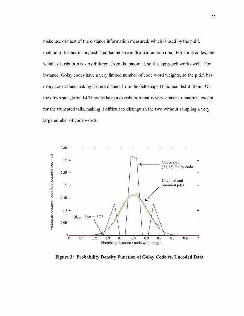
This p.d.f. approach is an improvement because it accurately estimates n for a given code
with less code words than the minimum distance technique. The latter method does not
22
make use of most of the distance information measured, which is used by the p.d.f.
method to further distinguish a coded bit stream from a random one. For some codes, the
weight distribution is very different from the binomial, so this approach works well. For
instance, Golay codes have a very limited number of code word weights, so the p.d.f. has
many zero values making it quite distinct from the bell-shaped binomial distribution. On
the down side, large BCH codes have a distribution that is very similar to binomial except
for the truncated tails, making it difficult to distinguish the two without sampling a very
large number of code words.
Coded pdf:(23,12) Golay code
Uncoded andbinomial pdfs
0 0.1 0.2 0.3 0.4 0.5 0.6 0.7 0.8 0.9 10
0.05
0.1
0.15
0.2
0.25
0.3
0.35
Hamming distance / code word length
(dmin � 1)/n = 6/23
Figure 3: Probability Density Function of Golay Code vs. Uncoded Data
His
togr
am o
ccur
renc
es /
tota
l occ
urre
nces
= p
df

23
The total number of code word measurements is similar to the minimum distance
technique, the only difference being that the required number of measured code words W
is reduced. However, code size is still the factor which determines whether a trial and
error search is feasible or not. Note that code word weight can be substituted in for
distance as in the minimum distance technique to reduced complexity somewhat.
Both distance techniques described above provide an estimate of the code word length n,
but they do not inherently provide any indication of the input word length k. The next
section discusses several techniques which do estimate both n and k inherently; hence the
code rate is derived in a single step. In particular, the last method presented will show
that the code rate can be derived using a simple trial and error search over n, without a
high dependency on size of the code.
2.3.1.2 Data Compression Techniques
Recall that FEC encoding adds redundancy to a data source in a controlled manner, and
the heart of our code rate estimation problem is to measure the entropy of an encoded
data stream. Data compression can be used to remove redundancy, so the obvious
approach for estimating entropy is to compress a data stream of sufficient length for the
compression algorithm to be effective. Then the resultant ratio of compressed length to
uncompressed length should roughly indicate the code rate.

24
An early attempt was made to compress coded data files using conventional software
based on the Lempel-Ziv dictionary compression algorithm. Results were erratic and did
not properly estimate the code rate for all but a few cases, even with very large files. The
source file was also checked to ensure it met the assumption of maximum entropy, and it
did not compress at all, as expected. So the obvious approach was initially abandoned in
favor of the distance techniques.
After some more thought, a simple modification was made to the universal dictionary
technique to tailor the compression to FEC encoded sources. Universal compression
typically uses a variable input word length to construct the dictionary, which does not take
advantage of the fact that FEC block codes have a fixed word length and furthermore a
constant amount of redundancy from word to word. A fixed word length dictionary can
be constructed at each trial value of n, such that the only trial length to compress
significantly is the actual code word length.
This modified dictionary compression technique can be summarized by the following
simple procedure:
1. Read an n-symbol word from the input stream, where n is the trial code word length;
2. Search the dictionary for this word; if it is not present, then add it to the
dictionary;

25
3. After processing W input words in this manner, check the dictionary length L; 4. If L is equal or close to qn then this was not the actual code word length; if it is
significantly less than qn, then this should yield the correct value of n as well as k; 5. If n was found in step 4, then estimate k = logq(L); 6. Otherwise repeat for all trial lengths of n until k is found; 7. If all trials produce a maximal dictionary length, then assume the source was not
FEC encoded.
This compression technique provides the exact value of k if and only if each word in the
code has been encountered. Furthermore, enough repeat words should be processed to
build confidence that the algorithm is actually compressing, after an initial stage in which
almost every word is added to the dictionary (this is true for any dictionary compression).
This is what allows us to differentiate coded from uncoded maximum entropy sources.
The latter do not compress at all, but may falsely appear to if the dictionary has not been
fully established. Hence, the accuracy of k and the compression reliability are dependent
on W, the number of words processed. Experiments have shown that values of W on the
order of qn give a correct estimate for all but very high rate codes, since qk is much smaller
than qn. As the code rate approaches one, less compression is achieved for coded sources,
so more words must be processed.
From the preceding arguments one may conclude that the modified dictionary
compression method is still highly dependent on code size, as are the distance techniques.
However, it does provide a rough estimate of k even if only a subset of all possible code

26
words is captured. But once again the computational requirements for complex codes
make this technique infeasible, due to the linear dependence on number of code words.
To overcome the implementation problems associated with distance and dictionary
compression algorithms for finding code rate, a new method was developed based on
matrix reduction. The general idea is to find a basis of the vector space in which the code
is defined. Keep in mind that a block encoder generator matrix G is a set of k basis
vectors which span the vector subspace of dimension k. Since the basis vectors are
linearly independent, all code words are formed as a linear combination of the rows of G.
A trial and error search for n may be executed similar to the dictionary compression
technique, but instead of building a dictionary of code words at each trial length we
perform a matrix reduction. Several well-known algorithms exist to reduce a W-by-n
matrix to its minimal form, known as Reduced Row Echelon Form (RREF). Such a
reduction yields a set of k linearly independent basis vectors for a block coded data stream,
or n basis vectors for a random data source. Therefore, the correct code word length
should be the only trial length to compress to significantly fewer than n words, similar to
dictionary compression. The code rate k/n is derived in a single test. The following
example illustrates the difference between coded and uncoded RREF matrices.

27
Table 1: Trial Code Word Matrix after Reduction for a Binary (7,4) Block Code at n = 7 1 0 0 0 1 1 1 0 1 0 0 1 0 1 0 0 1 0 0 1 1 0 0 0 1 1 1 0 0 0 0 0 0 0 0 0 0 0 0 0 0 0 0 0 0 0 0 0 0 0 0 0 0 0 0 0 0 0 0 0 0 0 0 0 0 0 0 0 0 0 0 0 0 0 0 0 0 0 0 0 0 0 0 0 0 0 0 0 0 0 0 0 0 0 0 0 0 0
Table 2: Trial Code Word Matrix after Reduction for Random Data at n = 7 1 0 0 0 0 0 0 0 1 0 0 0 0 0 0 0 1 0 0 0 0 0 0 0 1 0 0 0 0 0 0 0 1 0 0 0 0 0 0 0 1 0 0 0 0 0 0 0 1 0 0 0 0 0 0 0 0 0 0 0 0 0 0 0 0 0 0 0 0 0 0 0 0 0 0 0 0 0 0 0 0 0 0 0 0 0 0 0 0 0 0 0 0 0 0 0 0 0
Table 3: Trial Code Word Matrix after Reduction for a Binary (7,4) Block Code at n = 8 1 0 0 0 0 0 0 0 0 1 0 0 0 0 0 0 0 0 1 0 0 0 0 0 0 0 0 1 0 0 0 0 0 0 0 0 1 0 0 0 0 0 0 0 0 1 0 0 0 0 0 0 0 0 1 0 0 0 0 0 0 0 0 1 0 0 0 0 0 0 0 0 0 0 0 0 0 0 0 0 0 0 0 0 0 0 0 0 0 0 0 0 0 0 0 0 0 0 0 0 0 0 0 0 0 0 0 0 0 0 0 0 0 0 0 0 0 0 0 0

28
0 0 0 0 0 0 0 0
The matrix reduction algorithm is superior to the dictionary compression and distance-
based techniques since a much smaller percentage of code words is required to achieve an
accurate result. Recall that the other methods require W on the order of qn or greater,
since they are highly dependent on the code size. This method is dependent on the code�s
dimension k, not it�s size, since we are working with the vector basis instead of the entire
vector space. Testing has shown accurate results with W set to 2nλ, for a wide variety of
block codes. Note that the matrix reduction is always performed in GF(2) for simplicity,
but it works equally well for the nonbinary case if q-ary code words are left as a nλ-bit
sequence.
To illustrate the improvement in efficiency over the other techniques, consider searching
for code rate given a (63,57) Reed-Solomon encoded input bit stream. The size of this
code is 6457 (over 10100), and at least this many code words must be processed at each trial
length using the distance techniques just to find n. Dictionary compression provides an
inherent estimate of k in addition, but no significant improvement in complexity. Matrix
reduction requires only about 2*63*6 = 756 code words at each trial length to correctly
deduce the code rate. The RREF process itself involves up to W2 iterative operations per
trial length, versus less than WL for dictionary compression (L ≤ W), or WM for either
distance technique (typically M ≤ 10). Even with this increased processing load relative to

29
W, the RREF algorithm requires less than 106 total operations per trial length. RREF
matrix reduction is described further in section 3.3.1 since it was the winning algorithm for
code rate estimation.
2.3.2 Alphabet Size Estimation
Once the code rate has been established, the alphabet size q can be determined by
searching a range of λ (bits/symbol). Since the initial matrix reduction was done in GF(2),
the resulting code rate estimation actually represents kλ/nλ. We must find λ to determine
q, k, and n, but not the code rate itself.
The number of bits per symbol λ is swept from one to eight to cover binary through 256-
ary codes. At each trial value of λ another matrix reduction is performed, but first the
matrix of W nλ-bit words is transformed into a matrix of n-symbol words by grouping
every λ bits into a symbol. This time, the RREF algorithm modified for general GF(q)
arithmetic is used to compress the trial code words into a set of basis vectors. The trial λ
to achieve the greatest compression (i.e., lowest code rate) is declared the winner.
Generally, only one trial value should compress significantly, which indicates the correct
alphabet size q = 2λ. Note that this search only requires testing trial values of λ that
evenly divide into the previously estimated value of nλ. Also, the number of code words

30
per RREF trial was set to W = n + 10, and this was found to be adequate for all nonbinary
test cases.
No other algorithms were explored for deriving the alphabet size, but if a direct estimation
of q could be performed before the code rate estimation, then a significant increase in
performance would occur for nonbinary codes. This issue is discussed further in section
2.5 as an area for future study.
Table 4: Trial Code Word Matrix after Reduction for a 64-ary (63,57) Block Code at q = 64, n = 63 1 0 0 0 0 <columns 6-57> 0 0 43 32 40 50 2 58 0 1 0 0 0 <rows 1-57> 0 0 13 46 27 28 47 49 0 0 1 0 0 : 0 0 25 11 9 39 42 39 0 0 0 1 0 : 0 0 21 26 35 57 19 39 0 0 0 0 1 : 0 0 26 55 13 55 24 52 0 0 0 0 0 : 0 0 13 27 62 26 32 5 0 0 0 0 0 : 0 0 36 7 54 42 53 49 0 0 0 0 0 : 0 0 39 2 60 4 21 12 0 0 0 0 0 : 0 0 49 41 53 13 51 51 0 0 0 0 0 : 0 0 29 12 60 39 51 56 0 0 0 0 0 : 0 0 41 12 16 47 10 38 0 0 0 0 0 : 0 0 56 51 57 62 34 6 0 0 0 0 0 : 0 0 16 44 61 4 27 25 0 0 0 0 0 : 0 0 62 36 52 6 37 39 0 0 0 0 0 : 0 0 62 33 28 48 11 61 0 0 0 0 0 : 0 0 14 38 35 23 19 46 0 0 0 0 0 : 0 0 8 5 30 24 26 38 0 0 0 0 0 : 0 0 29 39 43 28 39 26 0 0 0 0 0 : 0 0 46 44 8 32 50 49 0 0 0 0 0 : 0 0 28 4 32 14 23 46 0 0 0 0 0 : 0 0 25 1 22 24 36 18 0 0 0 0 0 : 0 0 27 28 49 33 41 20 0 0 0 0 0 : 0 0 46 30 46 9 61 26 0 0 0 0 0 : 0 0 39 37 41 45 60 57 0 0 0 0 0 : 0 0 44 3 2 33 46 61 0 0 0 0 0 : 0 0 10 26 15 20 54 2 0 0 0 0 0 : 0 0 25 31 19 27 21 18 0 0 0 0 0 : 0 0 16 38 44 39 34 21 0 0 0 0 0 : 0 0 9 10 44 23 45 37

31
0 0 0 0 0 : 0 0 42 48 46 44 31 2 0 0 0 0 0 : 0 0 60 56 55 40 45 32 0 0 0 0 0 : 0 0 2 47 6 57 61 38 0 0 0 0 0 : 0 0 19 60 40 2 59 30 0 0 0 0 0 : 0 0 36 32 10 62 51 46 0 0 0 0 0 : 0 0 26 54 58 25 2 11 0 0 0 0 0 : 0 0 41 55 40 49 21 13 0 0 0 0 0 : 0 0 60 8 52 43 15 32 0 0 0 0 0 : 0 0 46 16 63 11 39 56 0 0 0 0 0 : 0 0 35 29 4 36 2 60 0 0 0 0 0 : 0 0 33 39 21 29 18 1 0 0 0 0 0 : 0 0 3 47 38 37 5 1 0 0 0 0 0 : 0 0 32 61 58 63 59 28 0 0 0 0 0 : 0 0 5 11 41 14 12 34 0 0 0 0 0 : 0 0 4 58 20 59 36 55 0 0 0 0 0 : 0 0 11 6 39 26 2 30 0 0 0 0 0 : 0 0 13 34 55 43 30 28 0 0 0 0 0 : 0 0 3 31 61 23 12 34 0 0 0 0 0 : 0 0 42 30 11 53 61 8 0 0 0 0 0 : 0 0 23 16 34 4 48 49 0 0 0 0 0 : 0 0 5 7 46 32 30 60 0 0 0 0 0 : 0 0 63 60 42 47 56 15 0 0 0 0 0 : 0 0 40 60 47 13 34 13 0 0 0 0 0 : 0 0 45 10 34 48 20 47 0 0 0 0 0 : 0 0 53 26 57 28 12 63 0 0 0 0 0 : 0 0 11 7 60 23 18 25 0 0 0 0 0 : 1 0 42 33 7 62 11 34 0 0 0 0 0 : 0 1 9 9 50 33 18 22 0 0 0 0 0 <all zeros, etc> 0 0 0 0 0 0 0 0
2.3.3 Root Search
Cyclic block codes are generated from a single generator polynomial g(x), which may be
factored into one or more minimal polynomials defined over the Galois extension field
GF(qm). In turn, these minimal polynomials may be factored into the product of one or
more first-order terms based on field elements of GF(qm). Each element is a root of g(x),
similar to generalized polynomial factors defined over an infinite field. Since a cyclic code
word c(x) is generated by polynomial multiplication of a message word m(x) by g(x), the
coded symbol sequence also contains roots corresponding to the Galois field in which the
code is based.

32
As a simple example, consider a basic (7,4) binary cyclic code defined over the extension
field GF(23), where α is an element of GF(8), and a seventh root of unity since α 7 = 1.
The generator polynomial in this case is chosen as the single minimal polynomial based on
the conjugacy class {α, α 2, α 4}, hence every code word has these three roots.
g(x) = x3 + x + 1 = (x+α)(x+α 2)(x+α 4)
c(x) = m(x) g(x) = m(x)(x+α)(x+α 2)(x+α 4)
Once the code word length and alphabet size are known, it is a straightforward procedure
for an FEC recognition system to derive the generator polynomial if the correct extension
field roots can be found. Fortunately, there is also a straightforward procedure for finding
the extension field roots of an arbitrary polynomial using an algorithm called the Galois
Field Fourier Transform (GFFT). This transform technique is explained in more detail in
section 3.3.2.1.
A block encoder may also be viewed as a feedforward linear system which has spectral
zeros in its transfer function due to the roots of g(x), just as a linear Finite Impulse
Response (FIR) filter has zeros in its transfer function H(f) to achieve the desired
frequency response. In the case of a block encoder, the desired �frequency response� is
one that separates output code words by a maximum distance, such that the decoder has

33
the greatest probability of correctly recovering the message words. In fact, several
decoding techniques are based on the spectral characteristics of cyclic block codes.
The basic approach used for identifying cyclic codes using the GFFT is simple but
extremely effective. Given that the alphabet size q, code word length n and frame starting
position are known, the GFFT of each code word can be calculated for a trial extension
field GF(qm). Each code word c(x) independently has roots due to both factors m(x) and
g(x), but only the roots of g(x) remain consistent from word to word since the input
message sequence m(x) is presumed random. Also, zeros in the GFFT spectrum only
appear for the roots of g(x) whenever the correct extension field (or a subfield thereof) has
been chosen.
With this information, the following search algorithm was developed:
1. Select a set of trial values of m to search, such that this set of primary fields covers all subfields of interest in an optimal manner (more on this partitioning later);
2. For each extension field GF(qm), determine the set of valid trial code word lengths
n such that qm-1 divides n evenly. This step is only required if the actual code word length has not already been determined. If n is known, search only the extension fields for which qm-1 divides n evenly.
3. For a given n and GF(qm), perform a cumulative GFFT over W1 code words. A
cumulative GFFT is calculated by logically OR-ing together the individual spectrum vectors for all code words. This has the effect of preserving spectral zeros which are present over all code words, and eliminating any zeros which are not always present. The number of code words to measure may be as small as W1 = 3 for good results in an error-free environment.

34
4. If any spectral zeros are present after step 3, repeat the cumulative GFFT test over a larger number of words W2. Thirty code words provide very accurate results in an ideal environment. This two-stage approach is used to improve the efficiency of the search algorithm. The quick zero test in step 3 weeds out most incorrect trials, while the second test validates surviving zeros over a longer observation interval to ensure they arise from g(x) and not a random recurrence of factors in m(x).
5. If no zeros remain after step 3, repeat that test for all trial lengths and extension
fields until consistent spectral zeros are found. 6. If all extension fields have been exhausted without finding consistent zeros, then
conclude that the symbol sequence has not been encoded by a cyclic block encoder and terminate the search.
7. If a valid extension field has been found in step 4, now search the set of trial values
of m representing all subfields of this primary extension field. The tests performed on these trial subfields are the same as those performed on the primary fields in steps 2-5. The trials are tested in order of smallest subfield to largest; return after the first subfield to pass both root tests. Note that if a given subfield of the current primary field has already been covered by a previous primary test which failed, then it is bypassed in the current subfield search.
8. If all extension subfields of the winning primary have been exhausted without
finding consistent zeros, then conclude that the cyclic code has been defined in the primary extension field.

35
START
Search primary fields m= 12,20,14,16,18,11,15
Search valid lengthssuch that (q^m-1) | n
NOT CODED
SUBFIELD
Roots found?No
Yes
Cum. GFFT:n, GF(q^m), 3 words
Cum. GFFT:n, GF(q^m), 30 words
More lengths? More fields?
No
No
Yes Yes
Roots found?
Yes
No
Search subfields(m depends on primary)
Save length n andextension field m
Optional:do not search validlengths if n is given
Search valid lengthssuch that (q^m-1) | n
PRIMARY FIELD
Roots found?No
Yes
Cum. GFFT:n, GF(q^m), 3 words
Cum. GFFT:n, GF(q^m), 30 words
More lengths? Moresubfields?
No
No
Yes Yes
Roots found?
Yes
No
Figure 4: Root Search Flowchart

36
2.3.4 Reconstruction of Cyclic Generator Polynomial
Once the correct extension Galois field GF(qm) has been identified for a sample code word
sequence using the root search method, the roots themselves can be used to reconstruct
the cyclic code�s generator polynomial. It is a very straightforward approach: the
generator polynomial is simply formed as the product of first-order polynomials based on
each root found. Consider the example given in the previous section, where the generator
polynomial roots are based on the conjugacy class {α, α2, α4}. First-order polynomials
are formed for the three roots as (x+α i), then multiplied together using GF(8) arithmetic
since this was the extension field in which the roots were found.
(x+α)(x+α2)(x+α4) = x3 + x + 1 = g(x)
Implementation details of the algorithm used to form this product are discussed in section
3.3.3.
2.3.5 Binary Cyclic Block Code Classification
The previous two sections focus on identification of cyclic codes down to the generator
polynomial. Cyclic codes may be either binary (i.e., alphabet size q = 2) or nonbinary (q
> 2), as determined by the search defined in 2.3.2. This section provides some methods to

37
further classify binary cyclic codes, once the extension field roots and generator
polynomial have been successfully identified.
First an integrity check may be performed to verify that the results derived to this point are
correct. Recall that the code rate R = k/n was determined via matrix reduction, and
therefore the code�s redundancy r = n-k. The redundancy can also be independently
derived as the degree of the generator polynomial (i.e., r = deg[g(x)]). If these two results
do not agree, then the code recognition system flags an error and may start a more
thorough search.
If the redundancy check does pass, then further classification is made into one of three
general types of binary cyclic block code: BCH, perfect, or general Cyclic Redundancy
Check (CRC). BCH codes can be identified by the presence of consecutive roots in the
Galois field spectrum, since their error correction capacity is defined by consecutive
powers of α as factors of the generator polynomial. Perfect codes fulfill the Hamming
bound with equality, and are categorized as binary repetition, Hamming, or Golay codes.
If the binary cyclic code fails to meet either of these criteria, then it is concluded to be a
general CRC code by default. Finally, note that these three subclassifications are not
mutually exclusive. For example, there exist perfect BCH codes, such as the (7,4) binary
BCH code which also qualifies as a Hamming code.

38
2.3.5.1 Binary BCH Codes
After specifying a cyclic code�s generator polynomial and verifying the redundancy, the
first test performed is to check for consecutive zeros in the cumulative GFFT spectrum.
The algorithm for isolating the largest group of consecutive zeros in the frequency vector
is described in section 3.3.4. If two or more consecutive roots are found in the largest
group, then it is concluded that the data source has been encoded by a binary BCH code.
The BCH design rule requires that there are twice as many consecutive powers of α as the
error correction capacity t. Therefore, t = z/2, where z is the number of consecutive
powers of α and t is the guaranteed number of bit errors that can be corrected in any code
word.
Another check can be made to ensure the integrity of our result. Since the minimum
distance of any FEC block code must be greater than 2t, this can be checked by directly
measuring dmin and verifying this relationship. Methods for estimating dmin were discussed
in 2.3.1.1, and recall that it becomes very difficult to accurately estimate the correct value
for large codes due to the tremendous number of code words required. However, the
estimate of dmin is always greater than or equal to the actual value. So the net effect is that
this is not a very accurate check when large codes are involved, but it will not
inadvertently invalidate our result as long as the estimate of t is correct.

39
Assuming everything is still valid at this point, one final check is made before declaring
that a binary BCH code has been used. Remembering the criterion that the length n of a
cyclic block code must divide evenly into qm-1, this is verified to ensure that the correct
identification has been made.
2.3.5.2 Perfect Binary Codes
A perfect block code is defined as one which satisfies the Hamming bound exactly. This is
a lower bound on the redundancy required for a length n q-ary code to correct t errors.
So for perfect codes we have the following equality:
r = logq{∑=
t
i in
0
(q-1)i}.
Specifically in the case of binary codes, q = 2 and the perfect code criterion can be stated
as:
r = log2{∑=
t
i in
0
}.
This calculation requires an estimate of n and t, and t can be derived from the code�s
minimum distance: t = floor[(dmin-1) / 2]. Once again, the accuracy of our estimate of dmin

40
is dependent on the code size, but fortunately perfect codes are limited in size so the
minimum distance can be correctly estimated with reasonable computation time.
Assuming we have identified a binary cyclic block code, estimated the exact value of dmin
and t, and have found that the redundancy meets the Hamming bound with equality, then
the code is declared to be in the class of perfect binary codes. This class has been proven
to contain only three subsets: binary repetition, Golay and Hamming codes. Further logic
can be used to easily subclassify a code into the correct group.
Binary repetition codes have the distinct property that k = 1, so this is the first check.
Furthermore, they must satisfy t = [(n-1) / 2]. If this is found to be true, then we conclude
that it is indeed a binary repetition code; otherwise, an error is declared since the other
possible perfect binary codes do not have k = 1. If k ≠ 1, then we check for the condition
that n = 23 and k = 12. If this is true and t = 3, then the system declares that it is a binary
Golay code; otherwise if this is true but t ≠ 3 an error is declared. Finally, the last test is
to check if n = 2m-1. If this is true and t = 1, then the system declares that it is a binary
cyclic Hamming code; otherwise if this is true but t ≠ 1 an error is declared.

41
2.3.5.3 Binary CRC Codes
On the contrary, if either of the estimates for dmin or t fail, or the redundancy check fails,
then we conclude that the code is not perfect and classify it as a general cyclic code. The
Cyclic Redundancy Check (CRC) is a common application for cyclic codes that do not
meet the other classifications. Therefore, since there are no further tests to try, an
intelligent guess would be to assume by default that the system has identified a CRC code
at this point.
2.3.6 Binary Noncyclic Block Code Classification
If the block code root search described in 2.3.3 failed to find consistent roots in any Galois
extension field GF(8) through GF(220), and the alphabet size q has been determined to be
2, then the FEC recognition system classifies this block code as a binary noncyclic code.
At this stage, finding the generator matrix G will completely specify the code. How to
find G is an open issue, and will be revisited in section 2.5. General binary Hamming
codes and Reed-Muller codes fall into this category.
2.3.7 Nonbinary Cyclic Block Code Classification

42
Once roots are found for a block encoded bit stream with q > 2, the appropriate extension
field GF(qm) and generator polynomial g(x) can be specified for this nonbinary cyclic block
code. As was the case for binary cyclic codes, the redundancy r can be double-checked as
the degree of g(x). If the two independent results agree, then the code may be
subclassified depending on certain properties.
2.3.7.1 Nonbinary BCH Codes
Similar to the binary BCH case, nonbinary BCH codes can be identified as having
consecutive roots in the extension field spectrum. Once again, by design a BCH code has
z = 2t consecutive roots, so the error correction capability may be derived as t = z/2.
Consecutive roots of a nonbinary BCH code may or may not be field elements of GF(qm),
depending on the length n. It is important to note that in the latter case, the search for
consecutive roots must be carried out using the nth roots of unity in GF(qm), not equivalent
powers of field elements α.
2.3.7.2 Reed-Solomon Codes
Reed-Solomon codes are a special case of nonbinary BCH codes, where the alphabet size
and code word length are matched to the extension field GF(qm) such that n = q-1 and

43
m = 1. These two conditions are checked to determine if the nonbinary BCH code is also
a Reed-Solomon code.
2.3.8 Nonbinary Noncyclic Block Code Classification
As in the binary case, if the bock code root search failed to find consistent roots in any
Galois extension field GF(8) through GF(220), but the alphabet size q > 2, then the FEC
recognition system classifies this block code as a nonbinary noncyclic code. Once again,
finding the generator matrix G will completely specify the code, but no methods have been
developed yet for determining G.
2.4 Convolutional Code Identification
Convolutional codes are in widespread use, but the search space is smaller (compared to
block codes) when considering only the most effective codes. Specifying a convolutional
code�s rate R, constraint length K, and generator polynomials gi(x) are required to
construct a proper decoder, where a rate R = k/n code has kn generator polynomials of
length K.2 The polynomials which provide the best distance properties and hence error
correction performance for a given rate, constraint length, and memory order are known.
2 For the general case when k > 1, some of the input delay lines may have fewer than K-1 delay elements. Hence multiple input convolutional codes also specify the total number of memory elements M. However, for our purposes we may consider all delay lines as maximum length, with generator tap values set to zero beyond the actual length of a given delay line where required.

44
A random search could be performed by which the recognition tool systematically tries
every possible combination of rate, constraint length and generator polynomials until a
Maximum Likelihood Sequence Estimation (MLSE) decoder converges to an optimal
solution3. Assuming an error free input bit stream, the sequence detector should yield the
best possible maximum likelihood path metric only when all decoder parameters match the
encoder. If only the best known generator polynomials are tried at every combination of R
and K, then a maximum of NR(Kmax � Kmin+1) trials must be run through the decoder. In
our limited search space, only NR = 5 rates are considered and K ranges from 3 to14, for a
worst-case total of 60 trials. Furthermore, each trial must consider nk! possible orderings
of generator polynomials, which ranges from 2 for a rate ½ code to 4.8x10⁸ for a rate ¾
code. Clearly the search becomes prohibitive for high rate, multiple input convolutional
codes.
If all possible generator polynomials are considered in each trial, instead of only the best
known, then the search space increases exponentially. Each length K generator has 2K
possible combinations of tap coefficients; hence there are 2Knk tap combinations in the
encoder when counting all polynomials. Cases where all taps for any given polynomial
3 MLSE decoding algorithms such as the Viterbi decoder generally exhibit convergence of the maximum likelihood path metric to the optimal value when the decoder�s input and output are error free. Conversely, no path metric should converge to the optimal value when the output is incorrect, either due to bit errors in the input stream, code word misalignment, or in our case a decoder which is not matched to the encoder.

45
equal zero may be ignored, reducing the total number of combinations to 2Knk - ∑=
nk
i ink
1.
Note that this result includes possible orderings, so the total complexity per trial ranges
from 26 � 3 = 61 for {R = 1/2, K = 3} to 2156 ≈ 1047 for {R = 3/4, K = 14}.
A parametric classification technique may be used to improve upon the random search
described above. The convolutional code identification problem may be decoupled into
two parts, by first searching for memory in the encoded bit stream, then searching for
generator polynomials. The advantage of such an approach is that the code rate and
constraint length may be derived without considering possible orderings or tap
combinations of the generator polynomials. Also, MLSE decoding is not required at every
trial since simple counting methods are adequate, as will be described shortly.
2.4.1 Memory Detection
The first part of the convolutional parametric search involves a joint search for the code
rate and constraint length. An initial approach to memory detection via autocorrelation of
the coded bit stream was investigated, since a convolutional encoder has similar structure
to interleaved FIR filters. However, this did not appear to be practical due to modulo-2
summation in the encoder, which effectively makes the memory introduced between bits
transparent when observing the output stream.

46
Two alternative methods were later developed, the second of which proved to be very
practical and effective. The first promising technique was based on forming a histogram
of occurrences of bit sequences of a given length, and it takes advantage of the trellis
structure inherent in convolutional codes. Although the trellis histogram algorithm was
somewhat successful, a better approach was developed by adapting the best block code
rate estimation technique to convolutional codes. It was found that data compression via
binary RREF matrix reduction can be used to determine the constraint length and code
rate of a convolutional encoded bit stream, if the results are interpreted correctly.
2.4.1.1 Trellis Histogram Technique
The trellis histogram search method was developed based on simple counting techniques.
The idea takes advantage of the trellis structure imposed on a convolutional encoded bit
stream. If enough coded bits are observed to cover the constraint length of the encoder,
then we should begin to see that the number of bit permutations remains consistently less
than the total number of permutations for a random memoryless sequence. This is
equivalent to saying that a convolutional encoder limits the number of possible paths
through the trellis to ensure that the minimum distance between possible output sequences
is greater than one, which is how its error correction property is derived.

47
As an example, consider a rate ½, K = 3 code whose two generator polynomials are
unknown. Assuming that frame sync provides us with correct alignment of the discrete
code words, the received bit stream may be divided into blocks of length nK, as shown in
figure 5.
C0 C5C4C3C2C1 .....
1 block: K = 3 symbols, n = 2 bits,2Kn = 64 permutations if no memory,2(K-1)n+1 = 32 permutations if coded
2 symbols = 4 bits,2(K-1)n = 16 permutations
1 symbol = 2 bits,2n = 4 random permutations,
but only 2 coded permutationsdue to trellis structure
Figure 5: Sequence Permutations for a Rate ½, K=3 Convolutional Code
If the received bit stream has no errors, then each block may be one of 32 possible bit
patterns due to the trellis structure shown in figure 6. A memoryless random bit stream
does not have this limitation, hence 64 bit patterns are possible. The code recognition
system may detect a convolutional coded sequence by forming a histogram of occurrences
of all possible length nK bit patterns, counted over W blocks. This test is performed at
trial values of nK, and the search sweeps over the allowed values of K and n. When the

48
correct value of nK is tested, the histogram for this example should yield no more than 32
distinct bit patterns, while incorrect trials should yield more than 32 patterns if W is large
enough.
State 0000
0
33
33
1
11
22
2
0
0
33
1
1
22
0
0
33
1
1
22
State 2
State 3
State 1
Figure 6: Trellis Diagram for a Rate ½, K=3 Convolutional Code
This technique was tested on several convolutional codes, and it produced the expected
results at the correct trial value for nK. However, histogram entries of zero occurrences
also appear at incorrect trials, particularly for constraint lengths longer than the actual
value of K. In hindsight, this is not surprising since the trellis should further limit the
number of possible sequences (with respect to all possible random sequences) for all trials
beyond the constraint length. This property is applied in the next section, which presents a
more efficient means for detecting memory in convolutional codes.

49
2.4.1.2 Data Compression Technique
A brief comparison of memory detection for convolutional codes to rate estimation for
block codes can be made. Recall that the best algorithm for finding the block code rate
was reduction of a matrix of code words to row echelon form. This exact operation is not
possible for convolutional codes, since the encoder output is essentially one continuous
code word (the length n blocks are too short). However, the trellis histogram technique
from the last section has a common feature to the RREF method. Namely, it is estimating
the encoder entropy by directly observing the reduced dimension of the vector subspace
for partial code words, whereas RREF measures the reduced dimension of the vector
subspace for complete code words (vs. the full dimension vector space for uncoded
words).
With that in mind, it appears that the block code rate estimation techniques may be applied
to convolutional codes if we work with partial code words of length nK instead of length n
blocks (the latter may be viewed as 2n-ary symbols, not code words). In particular, the
GF(2) RREF algorithm may be used to compress a matrix of partial code words to
estimate the encoder�s entropy. The result will not indicate the exact rate directly, as in
the case of block codes, since we are not working with complete code words. However,
the resulting matrix rank should always be less than nK at the correct trial block length.

50
As indicated by the trellis histogram method, compression should also be observed for
trials beyond the constraint length as well.
It was found that binary RREF matrix reduction can be used to determine the constraint
length and code rate of a convolutional encoded bit stream. Trials were run across all
code word lengths n and the constraint lengths K in the search space, and patterns were
extracted from the resulting compression curves. Analysis of these trends enabled an
algorithm to be developed which can determine the correct values of n and K based on a
few simple rules. A generalization of the rules for rate 1/n codes allows for determination
of the input word length k as well; hence complete specification of the code rate for an
arbitrary convolutional code is possible. Details of memory detection via RREF
compression are explained in 3.3.5.
2.4.2 Reconstruction of Convolutional Generator Polynomials
Once the convolutional code rate and constraint length are known, we must identify the nk
generator polynomials (including order) to specify the encoder structure completely. As in
the nonparametric random search one could run systematic trials through a tentative
MLSE decoder, in which certain combinations of generators are tested until the best path
metric indicates success. However, this is more work than required if the assumption of
no bit errors is valid.

51
There is a simple algorithm to recover the original message sequence based on
multiplication of the interleaved coded bit streams by inverse generator polynomials,
provided no channel bit errors occurred. This technique was modified to remove the data
content instead of recover it, for the purpose of finding the unknown generator
polynomials. A search can be carried out by substituting in trial inverse polynomials until
the sum of interleaved coded bit streams equals zero. This effect of canceling the data
content indicates that the correct inverse polynomials have been found, from which the
original generator polynomials may be recovered.
Considering the potentially huge number of trials to run, there is an advantage to the
proposed data cancellation approach over MLSE decoding at each trial. The
computational complexity per trial is very low, allowing an overall faster search. The data
cancellation technique is fully described in 3.3.6.
A polynomial root search analogous to the cyclic block code root search would offer a
tremendous computational advantage over random search, even with data cancellation.
Recall that the cumulative GFFT spectrum is computed over a matrix of code words in the
cyclic root search, and consistent zeros in this spectrum represent roots of the generator
polynomial. Application of this algorithm to convolutional codes is possible only under
certain restrictions.

52
Since the convolutional encoder output is one continuous code word, the entire stream
must be processed for roots to appear in the GFFT spectrum. However, a root search is
possible if a partial code word can be found in the bit stream which has nK zero bits on
either end (i.e., K zero symbols). Presence of these zeros ensure that the encoder memory
has been flushed before and after the partial code word. Figure 7 illustrates a case for our
example rate ½, K = 3 code in which the output stream may be divided cleanly into 3
segments. The middle segment thus represents an entire convolutional code word since
our observation guarantees that the encoder was at state zero at the start and end.
State 00 00
03
3 33
11 22
2
0 3
22
03
1State 2
State 3
State 100
2 1303 12222 0000000 3333 1... ...
K = 3 zero output symbols guarantee state 0
Segment 1 Segment 2 Segment 3
Single zero output symboldoes not guarantee state 0
Figure 7: Segmentation of a Rate ½, K=3 Convolutional Code Word

53
Finally, note that a GFFT-based convolutional root search must be performed on the
interleaved bit streams in GF(2), not on the composite symbols as shown above.
Reconstruction using the roots found for each stream of a rate 1/n code will yield the
generator polynomials directly, while roots found for each stream of a rate k/n code will
yield the modulo-2 sum of input generator polynomials corresponding to that stream.
Separation of this sum into the individual generators is left as an open issue.
2.4.3 Single Input Convolutional Code Classification
For the most part, the search techniques described above for convolutional codes have
been geared toward rate 1/n codes (i.e., single input bit per n output bits). The opening
argument in section 2.4 showed that searches become prohibitively complex for multiple
input convolutional codes. The general case for k > 1 is discussed further in the next
section.
Unlike block codes, there are no families of convolutional codes based on algebraic
theory, however several classifications can be made. As already implied, convolutional
codes may first be classified into single or multiple input codes depending on the value of
k. They may also be classified as either systematic or nonsystematic, but this distinction is
not very important since nonsystematic linear FIR convolutional codes always have better
distance properties than the counterpart systematic codes. Regardless, systematic codes

54
may be identified by observing the derived generator polynomials: the systematic
generators have a single tap connecting the input to output bit.
Convolutional codes may also be classified as feedforward or recursive, similar to FIR or
IIR digital filters, and linear or nonlinear. Recursive and nonlinear codes are out of the
scope of this project, however, some of the search techniques may apply to these types of
code. Future research of recursive and/or nonlinear convolutional codes would be useful,
since they are becoming increasingly popular in practice (e.g., trellis coded modulation and
turbo codes).
2.4.4 Multiple Input Convolutional Code Classification Finally there remains the issue of finding the input length k if a multiple input
convolutional encoder was employed. The basic RREF memory detection process applies
to rate k/n codes regardless of the value of k, but the specific parameter recovery
procedure could not be directly applied without modification. The first approach started
by assuming that a rate 1/n code had been used if memory is detected. Generalization of
the rules used to derive constraint length from the rate 1/n compression curves led to a
closed form solution for rate k/n codes as well.
The subsequent generator polynomial search is not carried out if the resulting estimate of k
is greater than one, since the search complexity would be prohibitive. This is true for the

55
rate 2/3 and ¾ codes under consideration, regardless of whether we search for the best
known generator polynomials or all possible tap combinations.
2.5 Areas for Future Study
I conclude section 2 with a summary of some open issues that were previously alluded to.
These are potential candidates for future research regarding the general problem of FEC
identification.
First, as mentioned in 2.3.2, a substantial improvement in performance could be obtained
for nonbinary codes by direct estimation of the alphabet size q. The current approach is to
find the code rate first by RREF compression in GF(q), but this search must be conducted
for all possible values of q in the search space. If λ = log2(q) were found beforehand, then
the search would only need to cover the possible values of n once.
Another unsolved issue is determination of the generator matrix G for noncyclic block
codes. Cyclic codes are based on a single generator polynomial for which we can find
roots, but noncyclic codes use k generator polynomials to form the rows of G.
Investigation of this problem has led me to believe that it is not possible to determine G
for an arbitrary noncyclic block code, since the encoder output is an unknown linear
combination of k unknown polynomials. This is a two-dimensional problem space, and

56
multiple combinations of input bit stream and generator matrix can produce identical
coded bit streams. Therefore, the exact determination of G is ambiguous unless the input
bit stream is known.
As discussed in the problem statement, the scope of this project does not address modified
linear codes (e.g., punctured, shortened), concatenated codes, interleaving, recursive
codes, or nonlinear codes. However, certain applications use these extensions of basic
coding theory, so future research of these topics would allow a wider range of operating
environment models.
Finally, the one unsolved problem within the scope of this project is determination of the
generator polynomials for multiple input convolutional codes. A trial and error search is
too large in general, even considering only the ordering of the best known generators.
One possible solution to this problem would be a root search via segmentation or use of
complete convolutional code words, as described in 2.4.2.

57
3. Implementation of a Prototype FECC Recognition System
Up to now I have talked about general methods for identifying Forward Error Correction
codes given no information about the encoder. This major section will describe the
application of these methods in a software FECC recognition system. The Matlab
development environment is described first, including its C code extension interface. Then
a high-level overview of system processing is depicted via flowchart, followed by a
detailed discussion of key algorithms. Finally, system limitations, performance, and open
issues are included.
3.1 Development Environment
The bulk of the software prototype was implemented in Matlab scripts, called M-files.
Matlab version 5.2 was used, including several functions in the communications toolbox.
The hardware platform was a 400 MHz Pentium II PC with 64 Mbytes of memory and 8
Gbyte hard disk. The Matlab Extension (MEX) interface was used to optimize two key
functions in C code, for greatly improved speed of execution. The MEX interface allows
C code functions to be called from the core Matlab program transparently, thereby
eliminating performance bottlenecks.

58
Although the Matlab communications toolbox includes many Galois field arithmetic
functions, I used a lookup table approach for most Galois field operations for more
efficient computation. Tables are generated at startup to represent all Galois fields of
interest, which store each field element vector as an integer instead of an array. Hence,
GF(qm) operations using the toolbox directly must access log2(qm) double-precision
numbers for each input argument, while the table approach requires only a single access4.
Two tables are used: a vector table for conversion from a field element symbol
representation to vector representation, and a reverse lookup table to perform the
opposite conversion. Symbol representation of Galois field elements are defined as: {0 →
0,
1 → 1, α → 2, α 2 → 3, �, α N-2 → N-1 }, where N = qm. As an example, the tables for
GF(8) based on the primitive polynomial α 3 + α +1 are listed below:
Vectors = [0, 1, 2, 4, 3, 6, 7, 5]
Symbols = [0, 1, 2, 4, 3, 7, 5, 6]
The following source code tables list all custom Matlab files comprising the final software
prototype implementation, including support files for signal generation and testing. Each
table entry states the source code file name, function call format including input and
output arguments, and a brief description of what the function does. Note that the GFFT

59
and RREF functions were also implemented in C code MEX files, in addition to Matlab
code directly.
Table 5: Source Code Files for Final Prototype M-file Function Description go2.m Main program FindMem6.m [ConvCWLenEst,InputLen
Est,ConstraintLenEst] = FindMem6(FileName,kmax,nmax,Kmax)
Detect memory to find convolutional code rate and constraint length
FindGenPolys.m [G2] = FindGenPolys(FileName, n,K)
Find convolutional code generator polynomials for rate 1/n codes
EstRate3.m [RateEst,CWLenEst,InputLenEst,AlphabetSizeEst] = EstRate3(FileName, nmin,nmax,lmax)
Estimate code rate via RREF compression
FindRoots.m [ExtFieldEst,roots, CWLenEst] = FindRoots(FileName, WordCount,q,n)
Find roots of the generator polynomial by searching for zeros in the Galois field spectrum
GFFT2.m [X] = GFFT2(x,WordCount,n,q, qm,mx)
Take Galois Field Fourier Transform of a code word block
CumGFFT2.m [Xcum] = CumGFFT2(x,WordCount,n,q,qm,mx)
Cumulative GFFT by taking logical OR of all frequency vectors
SumGFx.m [z] = SumGFx(x) Sum the elements of input vector using GF(q) vector addition (exclusive OR)
SearchLens.m [n] = SearchLens(qm1, nmin,nmax)
Calculate valid root search lengths for a given field GF(qm)
EstMinDist.m [dmin] = EstMinDist(FileName,n, q,WordCount)
Estimate minimum distance of a code
EstRedundancy.m redundancy = EstRedundancy(n,q,t)
Estimate the redundancy of a code w.r.t. the Hamming bound
choose.m [nck] = choose(n,k) n choose k function = n!/{k!(n-k)!} FindConsecRoots.m
[ConsecRoots,t] = FindConsecRoots( BaseRoots)
Find largest group of consecutive zeros in the Galois field spectrum
PolyGFx.m [v] = PolyGFx(roots,n, q,qm,mx)
Reconstruct cyclic generator polynomial from its Galois field roots
ReadFields.m Read all Galois field vector and symbol tables from file
4 Note that all numbers in Matlab, including integers, are stored as double-precision floating point values. The optimized C code functions improve Galois field operations even further by storing the bit-array vectors as actual integers.

60
ReadGFx.m [vectors,symbols] = ReadGFx(qm,mx)
Read the vector and symbol tables for a specific Galois field from file
SelField.m [vectors,symbols] = SelField(qm,mx)
Select the vector and symbol tables for a given Galois field
power2symGFx.m [y] = power2symGFx(x) Convert powers of alpha to symbols sym2powerGFx.m [y] = sym2powerGFx(x) Convert symbols to powers of alpha sym2bits.m [bits] =
sym2bits(symbols) Convert a q-ary symbol stream to a binary stream
bits2sym.m [symbols] = bits2sym(s,n,WordCount)
Convert a binary stream to a q-ary symbol stream
Table 6: Source Code Files for Test Signal Generation GenData.m Generate an encoded random symbol stream BlockEnc.m [m,c,WordsWritten] =
BlockEnc(FileName, WordCount,BlockCount, n,k,q,G,FileIO)
Block encode a random q-ary symbol stream and save output to file
BCH.m [n,k,M,q,G,H] = BCH(n,k,t,q,g)
Construct generator matrix for a BCH code (covers Reed-Solomon too)
Golay23.m [n,k,M,G,H] = Golay23(gen)
Construct generator matrix for a length 23 binary Golay code
Hamming.m [n,k,M,G,H] = Hamming(m)
Construct generator matrix for a systematic binary Hamming code
GenFields.m Generate all Galois field vector and symbol tables GenGFx.m [vectors,symbols] =
GenGFx(qm,mx) Generate vector and symbol tables for a specific Galois field
ReedMuller.m
[n,k,M,q,G] = ReedMuller(r,m)
Construct generator matrix for a Reed-Muller code
ConvEnc3.m [m,c,WordsWritten] = ConvEnc3(FileName,Word Count,n,k,K,G,FileIO)
Convolutionally encode a random bit stream via GF(2) convolution
Table 7: Source Code Files for Testing Algorithms EstCWL.m [dmax,delay] =
EstCWLen(Nmax,r, WordCount)
Estimate code word length by finding minimum distance between code words as the length is varied
EstCWL2.m Estimate code word length by finding the net difference between the distance p.d.f. and the binomial p.d.f.
binomial.m [pdf] = binomial(n,p) Generate a binomial probability density function EstRate.m Estimate code rate via dictionary compression EstRate2.m Estimate code rate via RREF compression compress.m [CompressedWords,
DictLen] = ( d )
Compress an encoded symbol stream using modified dictionary compression technique

61
compress(s,WordCount,n) RrefGF2.m [G,rank] =
RrefGF2(A,tol) Calculate the binary Reduced Row Echelon Form of input matrix
RrefGFx.m [G,rank] = RrefGFx(A,q,tol)
Calculate the general Reduced Row Echelon Form of input matrix in GF(q)
Spectrum2.m Calculate the GFFT for a code word block subfields.m Generate matrix of Galois subfield coverage FindMem.m Detect convolutional code memory via
polynomial deconvolution (rate 1/n only) FindMem3.m Detect convolutional code memory via direct
trellis histogram (rate 1/n only) FindMem4.m Detect convolutional code memory via binary
RREF compression (rate 1/n only) FindMem5.m Detect convolutional code memory via RREF
compression in GF(q), (rate 1/n only) FindConv.m Find convolutional code generator polynomials
via data cancellation (rate ½, K=3 example)
3.2 System Processing Overview
The FEC code recognition system was designed at a high level with both a software
architecture and a procedural flow of control. In general, software architecture is the
arrangement of processing tasks into discrete functions and modules (i.e., source code
files), and the implementation of those functions in an appropriate coding language. The
previous section laid out the software architecture for this prototype system. Procedural
flow of control dictates at a high level what sequence of events occur given a specific
input. I chose to present the procedural design as a set of standard software flowcharts,
shown in figures 8-11.

62
As discussed earlier, classifying a block coded bit stream involves determining the code
rate, alphabet size, extension field, and finally generator polynomial or matrix. This order
of events was chosen for the final prototype, but other sequences are possible (in fact, the
initial root search algorithm was designed for operation prior to finding the code rate or
alphabet size). Also note that further classification of exact codes, such as Reed-Solomon
or Golay, and nonessential parameters such as t is performed where possible for
completeness.
START
Search forconvolutional codes
DONE
Search forblock codes
Foundconv. code?
No
Yes
NOT CODED
DONEFoundblock code?
No
Yes
Figure 8: Top-Level Flowchart
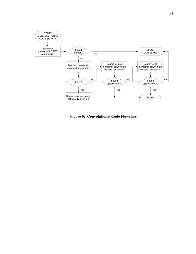
63
STARTCONVOLUTIONAL
CODE SEARCH
Search formemory via RREF
compression
Derive code rate k/nand constraint length K
Foundmemory? No
Yes
DONE
Foundgenerators?
No
Yes
Search for allgenerator polynomialsvia data cancellation
BLOCKCODE SEARCH
Revise constraint lengthestimate K given k, n
k > 1?
Search for bestgenerator polynomialsvia data cancellation
Foundgenerators?
Yes
NoNo
Yes
Figure 9: Convolutional Code Flowchart

64
START BLOCKCODE SEARCH
Estimate rate (n,k):RREF, GF(2),
search n = 7:255NOT CODED
Assume nonbinaryblock code
k=n for all n
k<n for one n(stop at first)
Find extension field roots:GF(8-1M) over GF(2)
Lowest R = k/nfor q=2
Found roots?
Find generator polynomialand verify rate:
g(x) = (x+r1)(x+r2)...(x+ri)r = deg[g(x)], k = n - r
Binary cyclic block code
Assume binarynoncyclic block code
No
Yes
Consecutiveroots?Binary BCH block code
Find error correctioncapacity:
t = consecutive roots / 2dmin >= 2t+1
Assume CRC or perfectcyclic block code
Yes
No
Find extension field roots:GF(8-1M) over GF(q) in
general (q > 2)
(Find generatormatrix G)
Found roots?
Nonbinary cyclic block code
Find generator polynomialand verify rate:
g(x) = (x+r1)(x+r2)...(x+ri)r = deg[g(x)], k = n - r
Estimate minimum distanceby direct measurement
dmin >=2t+1 ?
(q^m-1) | n ?
ERROR
DONE
Yes
Yes
No
No
No
Yes
n = q - 1,m = 1?
RS block code
Nonbinary BCHblock code
Consecutiveroots?
Yes
Yes
No
Assume nonbinarycyclic block code
Assume nonbinarynoncyclic block code
DONE
Assume binaryblock code
Estimate alphabet size q:RREF, GF(q),
search log2(q) = 2:8Lowest R = k/nfor q>2
No
BINARY PERFECTCODE SEARCH

65
Figure 10: Block Code Flowchart
CRC or perfectcyclic block code
Estimate minimum distance& error correction capacity:
t = floor((dmin-1) / 2)
Perfect code? Assume CRCblock code
k = 1?
n = 2^m - 1?
n =23,k = 12?
Binary repetitioncode
Binary Golaycode
Binary cyclicHamming code
t = 3 ?
t = 1 ?
t = (n-1)/2 ?
ERROR
OKNo
No
No No
No
NoNo
Yes
Yes
Yes
Yes
Yes
Yes
Yes
BINARY PERFECTCODE SEARCH
Figure 11: Binary Perfect Code Flowchart
3.3 Algorithm Development and Optimization
Several important low level algorithms require detailed explanation, due to their inherent
complexity or efficiency considerations or both. Two frequently called functions, namely
row echelon form matrix reduction and Galois Field Fourier Transform, were optimized

66
with respect to both algorithmic and coding efficiency for improved computational speed.
The Galois extension field root search was also improved by partitioning the search space
for optimal field coverage. Reconstruction of a cyclic generator polynomial from its roots
is done in a straightforward manner, by convolution of a cumulative product polynomial
with successive roots. Then I present a novel approach to finding the largest set of
consecutive roots in a Galois field spectrum via successive differentiation, which is used
for identification of BCH codes. Finally, algorithms are described for convolutional code
memory detection using RREF compression and generator polynomial search via data
cancellation.
3.3.1 Data Compression via Reduced Row Echelon Form
As derived in 2.3.1.2, the best algorithm for finding the code rate is based on reduction of
a matrix of trial code words to Row Echelon Form. This compresses the matrix to a set of
k linearly independent basis vectors if the data source is block coded and the correct trial
code word length n has been selected. The reduction is performed in GF(q) arithmetic
using a standard linear algebra technique called pivotal condensation. Note that nonbinary
code words are represented as binary words for the initial code rate search in GF(2), by
storing the q-ary elements as binary numbers.

67
The pivot technique was first derived by adapting the Matlab RREF function to GF(2)
algebra, then optimization in C code was carried out via the MEX interface. Since the
reduction is always performed on a binary matrix, significant optimization was achieved by
packing binary columns into sets of 32 bit words. This way, bit operations can be
performed on 32-bit unsigned integers, covering 32 columns of the matrix at once. For
example, adding two rows of a 100-by-32 matrix in GF(2) can be achieved by a single
exclusive-OR operation. The same task in Matlab requires 32 modulo-2 additions.
For the alphabet size search, the RREF algorithm was adapted to arbitrary GF(q) algebra,
a much more complex operation than binary matrix reduction. This function was also
ported to C code for greatly improved speed of execution. Further optimization via bit
packing was not done for the general case of q > 2.
3.3.2 Extension Field Root Search
The key algorithm to identifying a cyclic block code is the Galois Field Fourier Transform
(GFFT), which is used to find roots of the code generator polynomial g(x). This transform
is defined in the next section, which also discusses optimization of the GFFT. The second
subsection then describes in detail a partitioning of the extension field search space for
efficient calculation via the GFFT.

68
3.3.2.1 Galois Field Fourier Transform
The GFFT is analogous to the Discrete Fourier Transform (DFT) for discrete-time signals
whose sample values are defined over an infinite field. The DFT produces a spectral
representation of a time-domain sample sequence, where the relative strength of each
complex exponential frequency (i.e., power of ejω) occurring in a sample block is
calculated. Similarly, the GFFT produces a spectral representation of a polynomial-based
symbol sequence whose values are defined over a finite field GF(q). The relative strength
of each field element (i.e., power of γ i) occurring in an n-symbol code word is calculated
to produce an n-point frequency vector consisting of elements in GF(qm).
The Galois Field Fourier Transform is defined as follows:
Vj = ∑−
=
1
0
n
i[γ ij vi],
where vi are symbols of the time-domain input vector, and Vj are symbols of the resultant
frequency-domain vector. The length n of the input and output vectors must divide evenly
into qm-1, since the element γ (whose frequency multiples we are measuring) is an nth root
of unity in GF(qm). Hence the roots of g(x) will appear only when the correct combination
of code word length n, base field GF(q), and extension field GF(qm) have been specified
for the GFFT calculation.

69
The DFT calculation can be significantly optimized via the Fast Fourier Transform (FFT)
algorithm. The FFT takes advantage of the periodicity of the complex exponential term
WN = e-j(2π/N), since WNN = e-j2π = 1. Similarly, the GFFT may be optimized to take
advantage of the periodicity of γ since it is an nth root of unity. Therefore, γ ij = γ i(j+n) = γ
(i+n)j
and the FFT optimization approach is valid for the finite field case.
However, an important distinction exists, namely the fact that the GFFT length n is an odd
number for practical codes. The most efficient FFT algorithms rely on decimation of the
time-domain signal or frequency domain spectrum vector by powers of 2, hence a length
N which is a power of 2 is highly desirable. For the infinite field case, an arbitrary time-
domain signal may be zero padded to extend its length to the closest power of 2, and the
frequency vector is typically chosen to be the same length. Therefore decimation in time
or frequency may be iteratively applied to achieve maximum efficiency (i.e., the FFT is
broken down into a series of 2x2 butterfly operations).
In the finite field case, on the other hand, the frequency vector length is not arbitrary and
must be equal to the code word length n in order to find roots. Therefore, the decimation
in frequency algorithm is not practical for GFFT implementation, but decimation in time
can be used by zero padding the input code word length to a power of 2. Zero padding

70
the time-domain code word does not affect the result; also, in many cases adding only a
single zero is sufficient to extend the length to a power of 2.
An optimized version of the current C code GFFT function using a basic decimation in
time approach could be used to achieve significant processing improvement in the
extension field root search. Other GFFT optimization techniques based on polynomial
algebra could also be implemented, for example, the method described in [14]. This
optimization is left as an open issue for further prototype development.
3.3.2.2 Extension Field Search Space
The first step in the root search algorithm presented in 2.3.3 mentioned a partitioning of
Galois extension fields into primary and subfields. In general, a Galois field GF(qm) can be
represented by elements of larger fields based on multiples of m. Likewise, any so-called
primary field GF(qmI) has elements which are shared by subfields GF(qmi), as long as mi
divides evenly into mI. If a given primary field shares elements with various subfields,
roots and hence spectral zeros are also visible in those fields.
For example, the (63,47) binary BCH code is defined in GF(64), where n = qm-1 = 63 and
m = 6, q = 2. The following extension fields share elements with GF(26), and therefore
roots may be found in any of these fields:

71
Table 8: Galois Subfields
i mi qmi-1 = ni ni / n Field element 1 6 63 1 γ 2 12 4095 65 β 3 18 262143 4161 α <etc.> : : : :
As an illustration, consider the case I = 2 and i = 1. Let β be an element of order 4095 in
GF(212), such that β4095 = 1. All powers of β from 0 to 4094 are elements of GF(4096).
Since n2 = 65n, define γ = β65 as an element of order 63 in GF(26) such that γ63 = β4095 = 1.
Hence β65 is also an element of the subfield GF(64), since m = 6 divides evenly into 2m =
12. GF(64) in this representation contains the elements {0, β0, β65, β130, β195,�, β4030}
which are equivalent to the set {0, γ0, γ1, γ2,� γ62}.
Likewise, let α be an element of order 262143 in GF(218) for the case I = 3. Since n3 =
4161n, define γ = α4161 as an element of order 63 in GF(26) such that γ63 = α262143 = 1.
Hence α4161 is also an element of the subfield GF(64), since m = 6 divides evenly into 3m
= 18. Note that a similar relationship does not exist between GF(218) and (212), since 12
does not divide evenly into 18.
Coverage of subfields by selected primary fields in the range GF(24) to GF(220) is shown
graphically based on the factorization of m for each field. Each column shows which

72
subfields in the range m = 3 to 10 are covered by each choice of primary search field from
m = 4 to 20. This table aided in choosing an optimal root search space such that the
fewest Galois Field Fourier Transforms are performed on average. Note that prime values
of m cannot be factored and have no subfields; also, GF(2) and GF(4) are not considered
since the minimum search length is 7.
Table 9: Extension Field Coverage Map
m 4 5 6 7 8 9 10 11 12 13 14 15 16 17 18 19 20 3 X X X X X 4 X X X X X 5 X X X X 6 X X X 7 X X 8 X X 9 X X 10 X X
Due to the inherent repetition of roots in multiply related fields, the root search may be
optimized by selecting a number of primary fields from the coverage table to search
initially. These fields were chosen to cover the set of all Galois fields from m = 3 to 20,
with three selection criteria. The search is strategically ordered such that primary fields
covering the most subfields are tested first, with as little redundancy as possible, and
otherwise in order of ascending field size. The chosen search order and coverage is
illustrated by the following table, with redundant subfields shown in parentheses:

73
Table 10: Optimal Extension Field Partition
Primary field 2m Primary m Subfields m Factorization of m 4096 12 3, 4, 6 2*2*3 1048576 20 (4), 5, 10 2*2*5 16384 14 7 2*7 65536 16 (4), 8 2*2*2*2 262144 18 (3, 6), 9 2*3*3 2048 11 - - 32768 15 - -
If the extension field search is performed without knowledge of the code word length n,
then certain trial values of n are searched at each trial extension field. However, unlike the
general code rate estimation problem where all lengths within some range are searched, in
this case the trial lengths are restricted. Only values of n which divide evenly into qm-1
must be considered, due to the construction of cyclic codes. The table below enumerates
all valid search lengths from n = 7 to 255 for all binary extension fields from m = 3 to 20.
Note that the prime values 13, 17 and 19 have no valid lengths, and therefore are not
included in the extension field search.
Table 11: Extension Field Search Lengths
Primary field 2m Primary m Valid lengths n 4096 12 7, 9, 13, 15, 21, 35, 39, 45, 63, 65, 91, 105, 117, 195 1048576 20 11, 15, 25, 31, 33, 41, 55, 75, 93, 123, 155, 165, 205 16384 14 43, 127, 129 65536 16 15, 17, 51, 85, 255 262144 18 7, 9, 19, 21, 27, 57, 63, 73, 133, 171, 189, 219 2048 11 23, 89 32768 15 7, 31, 151, 217

74
3.3.3 Reconstruction of Cyclic Generator Polynomial from Roots
Section 2.3.4 described at a high level the approach by which a cyclic code�s generator
polynomial g(x) may be reconstructed from roots in GF(qm). Here the mechanics of
forming g(x) from these roots are described in detail. Recall that the generator polynomial
is simply formed as the product of first-order polynomials based on each root found.
g(x) = ∏i
(x+γ i), where γ is an nth root of unity in GF(qm).
Polynomial multiplication is equivalent to convolution of the polynomial coefficients,
which in our case are powers of γ. Hence, this product is formed algorithmically as
follows:
1. Convert the nth roots of unity in GF(qm) to primitive field elements (i.e., qm-1 roots of unity) by multiplying the exponent by (qm-1)/n;
2. Multiply the first two first-order polynomials together by convolving the
coefficient vectors in GF(qm), resulting in a second-order polynomial; 3. Multiply the previous resultant polynomial with the next first-order term, via
convolution; 4. Repeat step 3 until all terms have been multiplied together to form g(x).
5. Convert the polynomial coefficients from primitive elements in GF(qm) back to
GF(q) by multiplying the exponent by (q-1)/(qm-1).

75
As an example, consider the (21,15) 4-ary BCH code, where γ is a 21st root of unity in
GF(43) and α is a primitive element of GF(64). Since the GFFT is performed over length
n code words in the root search, step 1 converts the resulting roots γ to elements α for
convolution in GF(64). Step 5 has no effect for this particular example, since all
coefficients of g(x) are binary; however, this is not always the case so the conversion must
be performed in general.
3.3.4 Consecutive Root Search
Once it has been established that a cyclic code has been found due to finding consistent
roots in some extension field, then the placement of those roots may be observed to
determine if a BCH code has been found. In particular, BCH codes have 2t consecutive
spectral zeros by design. Other zeros may exist in the spectrum for certain BCH codes
outside the designed group of consecutive roots, either individually or in smaller groups.
An algorithm was developed to isolate the largest cluster of consecutive roots using a
differentiation approach.
The basic algorithm takes successive derivatives of an array of roots, represented as
powers of α. Each time the first difference is calculated, the resulting array contains a one
between each pair of consecutive roots. Then the index of all ones in the resultant array is
used to replace the previous array of roots, which at this stage now represents only roots
occurring in groups of two or more. Then the new array is differentiated, and the index of
all ones is again used to replace the previous array. The array size is shortened in each

76
step, and this procedure is repeated until there are no ones left in the resultant array. The
final result is the starting index and size of the largest group of roots. The size is
determined by the number of differentiations performed.
As an example, consider the array of roots for a (63,45) binary BCH code expressed as
powers of α, shown in step 1 of the table below. The first difference of this array
indicates three clusters of consecutive zeros (1-6, 16-17, and 32-34). Six successive
iterations are required to complete the search, and the resultant root array at each stage is
shown below. The largest cluster contains 6 successive roots, as indicated by the number
of iterations performed.
Table 12: Consecutive Root Search
Step Root Array First Difference 1 [1 2 3 4 5 6 8 10 12 16 17 20 24 32 33 34
40 48] [1 1 1 1 1 2 2 2 4 1 3 4 8 1 1 6 8]
2 [1 2 3 4 5 16 32 33] [1 1 1 1 11 16 1] 3 [1 2 3 4 32] [1 1 1 28] 4 [1 2 3] [1 1] 5 [1 2] [1] 6 [1] -
3.3.5 Memory Detection via Reduced Row Echelon Form

77
The winning algorithm for detection of convolutional codes is data compression via RREF
compression in GF(2). Trials are run for various values of n and K, and
RREF compression is applied to a matrix of nK-bit partial convolutional code words at
each trial. The values tested are n = 2, 3 and 4, and K ranging from 3 to 14, since these
are the values most commonly found in practice.
It was observed for all trials in the search space that the compression ratio Γ is a
monotonically decreasing function of K, given the correct value of n or integer multiples
of n. Other values of n may yield compression at some values of K, but Γ does not
consistently decrease. An example test case is shown below, in which RREF compression
is applied to a rate ½, K = 9 convolutionally encoded bit stream for all trials. Note that
the rate ½ and ¼ trials both exhibit monotonically decreasing compression ratios, starting
at the point where nK ≥ 18 (2*9 = 18 for the correct trial code rate, 4*5 = 20 for the
incorrect trial).

78
2 4 6 8 10 12 140.6
0.65
0.7
0.75
0.8
0.85
0.9
0.95
1
Constraint Length (K)
RREF Compression
Rate 1/2Rate 1/3Rate 1/4
Figure 12: Binary RREF Compression Trials for a Rate ½, K = 9 Convolutional Code
Based on these observed patterns, correct values of n and K may be derived for rate 1/n
codes by a simple interpretation of the RREF compression trials. First, the correct value
of n is the smallest trial value to result in a monotonically decreasing function of K.
Second, once n has been determined, the correct value of K is the trial at which the
compression ratio first drops below the threshold value of 2/n. In the previous example,
this threshold is equal to one, since n = 2. The other two cases considered have thresholds
of 2/3 and ½, for rate 1/3 and ¼ codes, respectively.

79
Extension of these rules to the general case of rate k/n codes was possible by observing
compression curves for rate 2/3 and ¾ codes. First, the threshold value in general is
(k+1)/n, which is in agreement with results above, and also indicates a threshold value of
one for rate ½, 2/3, and ¾ codes. The second modification involves the trial where the
compression ratio Γ first drops below the threshold. In general, this trial constraint length
Kest actually represents k(K-1)+1, which evaluates to K when k = 1. For cases when k > 1,
the actual value of K may be derived as [(Kest-1)/k]+1.
Finally, a third critical observation was required to deduce k directly, without an additional
search loop. Define the compression ratio Γ = kK/nK and ∆(K) = nK-kK = (n-k)K.
The function ∆(K) represents the difference between compressed and uncompressed
words at trial values of K; the first difference of ∆ is ∆’ = ∆(K) - ∆(K-1) = n-k. The
derivative ∆’ is calculated with each successive trial, and when the compression ratio
begins to monotonically decrease its value accurately represents n-k (provided the correct
trial value of n). Thus k may be recovered under these conditions as n-∆’.
Due to the required logic to simultaneously search for n, k, and K, sometimes the estimate
of K was corrupted for multiple input convolutional codes. A simple solution was
implemented to make a second search pass through all constraint lengths only, once the

80
values of n and k (and hence the exact threshold) are known. The combined techniques
proved effective for all arbitrary rate k/n codes that were tested (i.e., rate ½ through 3/4).
One important feature is that this binary RREF technique is robust against false
identification of block codes. The inherent memory in a convolutional code is required to
produce a monotonically decreasing compression ratio versus constraint length. As seen
in the block code rate testing, binary RREF compression of a block code will produce
values less than one only at multiples of nλ, where n is the actual block code word length,
and λ = log2(q). This is important because the search for convolutional codes precedes
the block code search; therefore, the memory detection test must fail for all uncoded or
block coded bit streams.
3.3.6 Reconstruction of Convolutional Generator Polynomials via Data Cancellation
Once the convolutional code rate and constraint length are known, we must identify the nk
generator polynomials (including order) to specify the encoder structure completely. As in
the nonparametric random search one could run systematic trials through a tentative
MLSE decoder, in which certain combinations of generators are tested until the best path
metric indicates success. However, this is more work than required if the assumption of

81
no bit errors is valid. In [5] it was shown that there exist a set of polynomials ai(x) such
that
∑−
=
1
0
n
iai(x) gi(x) = 1,
∑−
=
1
0
n
iai(x) ci(x) = ∑
−
=
1
0
n
iai(x) gi(x) m(x) = m(x).
Hence the original data word m(x) can be recovered by multiplying each interleaved
generator polynomial gi(x) by an inverse polynomial ai(x), provided the channel code word
c(x) is uncorrupted. This technique was modified to remove the data instead of recover it,
for the purpose of finding the unknown generator polynomials:
[∑−
=
1
0
n
iai(x) gi(x)] mod n = 0,
[∑−
=
1
0
n
iai(x) ci(x) = ∑
−
=
1
0
n
iai(x) gi(x) m(x)] mod n = 0.
Solution: ai(x) = ∏≠ij
gj(x),
[∑−
=
1
0
n
iai(x) ci(x) = ∑
−
=
1
0
n
i{∏
≠ij
gj(x)} gi(x) m(x) = ∑−
=
1
0
n
i{∏
−
=
1
0
n
j
gj(x)} m(x)] mod n =
0.

82
A search can now be carried out by substituting in the product of trial generator
polynomials until the sum of interleaved coded bit streams equals zero. Note that modulo-
n summations are used instead of modulo-2, to force a zero result for odd values of n;
polynomial products are still formed in GF(2). Also, the zero test should be validated
over at least two nK bit blocks, so that the n(K-1) bit convolution startup transient may be
ignored5. A practical search approach would be to start with the best known generators
and test all possible orderings until a winner is found. If this fails, a more thorough search
is required by testing all permutations of generator coefficients.
Considering the potentially huge number of trials to run, there is an advantage to the
proposed data cancellation approach over MLSE decoding at each trial. Data cancellation
involves only polynomial multiplication and modulo-n summation. MLSE decoding at
each trial would be more complex, even with the efficient Viterbi algorithm.
3.4 Areas for Future Prototype Development and Performance Improvement
The software prototype FEC code recognition system was developed in Matlab and two
performance bottlenecks were optimized in C code. Further performance improvement
could be realized by implementation of the RREF and GFFT functions in dedicated
5 Binary polynomial multiplication is equivalent to convolution in GF(2). As with a linear FIR filter, the convolution output includes a startup transient of length consistent with the filter memory. Therefore, the

83
hardware, yet retaining software control over most of the processing. For example, a
commercially available multiprocessor Digital Signal Processing (DSP) card could be used
to improve upon the PC environment, since DSPs are optimized for fast
multiplication/addition and modulo operations. It is doubtful that custom hardware would
yield much benefit, since the nature of the problem requires great flexibility in changing
parameters.
The GFFT algorithm itself can also be optimized similar to the FFT or via algebraic
techniques. The issues involved with this particular task were described in section 3.3.2.1.
Additionally, the nonbinary RREF algorithm could be somewhat optimized for a more
efficient C code implementation, since this is a time consuming operation.
Note that the current prototype was tested with generated test signals only, not actual
recorded signals. Another item for future prototype development would be to identify
several actual FEC encoded bit streams, provided that the captured data meets the
operating criteria stated in 2.1. Finally, identification of test signals and actual signals in
the presence of bit errors would prove the robustness of the parametric search algorithms.
zero test output is always zero only if we begin at the start of the entire convolutional code word; otherwise, entering �mid-stream� results in nonzero outputs until the delay line memory is filled.

84
4. Results
The prototype recognition system was repeatedly tested throughout development to aid in
debugging the software. Matlab files were developed to generate encoded test vectors,
which were used to test algorithms individually and then integrate the best ones into a final
working system. The set of test vectors that were generated is enumerated in section 4.1,
and then performance results are presented in 4.2. More specifically, performance results
are categorized into accuracy of code recognition, and speed of algorithm processing for
each test case.
4.1 Test Code Set
The set of 18 codes chosen for system development and testing is listed in the following
table, plus an uncoded �control� test case. The amount of data generated for each test
vector was roughly determined by the recognition system operating parameters. Generally
speaking, the more complex the code, the more data is required to detect it. Note that
random q-ary symbols were used as input to each encoder.

85
Table 13: Test Codes
Test # Code Type n k q m qm t K 0 Uncoded N/A N/A 2 N/A N/A 0 N/A 1 Hamming 7 4 2 N/A N/A 1 N/A 2 Hamming 15 11 2 N/A N/A 1 N/A 3 Golay 23 12 2 11 2048 3 N/A 4 CRC 7 4 2 3 8 1 N/A 5 BCH 63 45 2 6 64 3 N/A 6 Reed-Muller 16 5 2 N/A N/A 3 N/A 7 BCH 21 15 4 3 64 1 N/A 8 BCH 21 12 4 3 64 2 N/A 9 BCH 85 73 16 2 256 3 N/A 10 Reed-Solomon 63 57 64 1 64 3 N/A 11 Reed-Solomon 255 245 256 1 256 5 N/A 12* Convolutional 2 1 2 N/A N/A N/A 3-9, 14 13* Convolutional 3 1 2 N/A N/A N/A 3, 8, 14 14* Convolutional 4 1 2 N/A N/A N/A 3, 7, 14 15** Convolutional 2 1 2 N/A N/A N/A 9 16** Convolutional 3 1 2 N/A N/A N/A 4 17* Convolutional 3 2 2 N/A N/A N/A 3, 6 18* Convolutional 4 3 2 N/A N/A N/A 4 * Convolutional codes with best known polynomials and maximal memory order M ** Convolutional codes with suboptimal polynomials
4.2 System Performance Results
Performance of the final prototype FEC code recognition system was measured by running
the tests cases in table 13 through the Matlab main program. This section summarizes
system performance with respect to time of computation and accuracy of code parameters
recovered.

86
4.2.1 Code Recognition Performance
Overall, the accuracy of code recognition was exactly as expected for most codes tested,
since the algorithms were tested in an error-free environment. Recall that the goal of this
prototype testbed was to prove that the techniques are fundamentally sound. I believe that
the current algorithms can be modified or repeatedly applied to provide near perfect
performance for low but nonzero bit error rates; this was mentioned as an open issue in
section 3.4.
Note that all code parameters are not critical to successfully decode a bit stream, however,
the system attempts to derive as much information as possible to classify a given code.
The following six parameters are considered critical: n, k, q, m (cyclic codes only), K
(convolutional codes only), and g(x) or G. From these parameters one can directly derive
other parameters: n and k imply code rate R and redundancy r; alphabet size q implies λ
bits/symbol; m implies the Galois extension field for cyclic codes; and the generator
polynomial(s) or matrix imply the parity check polynomial h(x) or matrix HT or trellis
structure.
In contrast, there are several parameters which are not critical and cannot be derived
directly from the critical code parameters. These include the error correction capacity t,
minimum or free distance, and memory order M (convolutional codes only). By
noncritical it is meant that these parameters are not required to construct a working

87
decoder, but they may be useful properties to know for other reasons. For example, M
implies the number of states in a convolutional encoder and hence the required minimum
complexity of a matching Viterbi decoder. M is not a critical parameter since a working
decoder can be constructed with more than the minimum number of states, but it could be
used to reduce the recovered state machine to an optimal size, thus reducing the trellis
decoding complexity.
With the concept of critical and noncritical parameters in mind, specific results of system
testing were as follows:
• The uncoded test case failed the convolutional memory test and block code
compression test as expected, successfully indicating a rate 1 uncoded bit stream.
• All but one parameter for the noncyclic binary Hamming codes (test cases 1 and 2)
were correctly identified. No estimate of the generator matrix G was provided, but
this does not appear possible (recall section 2.5). Correct classification as a perfect
binary Hamming code was achieved in both cases, with t = 1 derived from dmin = 3.
• The binary Golay code was falsely classified as a 2 error correcting BCH code due to
consecutive roots in its spectrum. However, all critical parameters were correctly
identified (n, k, q, m, and g(x)), as was the minimum distance of 7.
• The binary CRC code in case 4 was correctly classified as a BCH code (note that they
are not mutually exclusive and it is also a Hamming code as well). All parameters
were correct.

88
• All six BCH codes (cases 5, 7-11) including the special case Reed-Solomon codes
were correctly classified and all applicable parameters were recovered. The minimum
distance estimates provided for these codes were not accurate for reasons examined in
2.3.1.1, but dmin is not even known for some BCH codes due to their large size.
• The (16,5) Reed-Muller code in test case 6 initially failed to recover the correct code
rate, since compression was encountered before the actual code word length
(estimated k = 4 at n = 8). The code rate search was modified to continue searching
after the first trial to show significant compression, as long as subsequent trials showed
higher compression. This change allowed accurate estimation of n, k and q, but then
the root search incorrectly classified it as a cyclic code due to roots found in GF(8).
However, this failure was caught by the redundancy check described in 2.3.5.
• The rate 1/n convolutional codes in test cases 12-16 were successfully identified, and
n, K and G were accurately recovered (where G is a matrix representation of the n
generator polynomials). Note that the polynomial search order was varied during
testing for cases 12-14, as was the order of trial tap permutations for cases 15 and 16,
in order to validate robustness of the search algorithms. No attempt was made to
estimate the minimum free distance.
• The rate 2/3 and ¾ multiple input convolutional codes in test cases 17 and 18 were
also successfully identified, and n, k, and K were accurately recovered for several test
constraint lengths. These codes were constructed using the best known generator

89
polynomials of maximal memory order M = k(K-1). No attempt was made to search
for the generators due to the complexity issue.
4.2.2 System Speed Performance
Time trials were performed during final testing to measure algorithm and implementation
efficiency. Most test cases were completed in several seconds, but several nonbinary BCH
codes and one convolutional code with suboptimal generators took up to 15 minutes.
Note that the timing results shown in table 14 do not include the time required to read in
the Galois field lookup tables. This task only takes several seconds, and is only performed
on the first trial after starting Matlab.
The third column below shows the execution time prior to fixing the initial problem with
the Reed-Muller code, while the fourth column shows results after changing the block
code rate estimation routine. This fix does not affect the convolutional code trials, and
adds roughly 20 seconds on average to the block code trials which did not involve an
extensive rate search to begin with.

90
Table 14: Recognition Time Trials
Test # Code Type Time (min:sec) 0 Uncoded 13:26 13:26 1 Hamming 0:04 0:22 2 Hamming 0:04 0:22 3 Golay 0:06 0:22 4 CRC 0:01 0:19 5 BCH 0:02 0:20 6 Reed-Muller - 0:18 7 BCH 0:01 0:19 8 BCH 0:01 0:19 9 BCH 3:34 3:35 10 Reed-Solomon 7:27 7:29 11 Reed-Solomon 15:13 15:14 12 Convolutional 0:01 0:01 13 Convolutional 0:01 0:01 14 Convolutional 0:01 0:01 15 Convolutional 14:18 14:18 16 Convolutional 0:13 0:13 17 Convolutional 0:01 0:01 18 Convolutional 0:01 0:01

91
5. Summary
In conclusion, a general parametric classification methodology was developed in this thesis
to reconstruct an error correction encoder from its output bit stream only, given no
information about the coding scheme used. Algorithms were developed in an intuitive
fashion, mainly using linear algebra principles and finite field arithmetic. An FEC code
recognition prototype testbed was built to experiment with different techniques for
extracting features from a coded sequence to determine the encoding parameters. This
system must also differentiate between block, convolutional, and uncoded bit streams.
A number of different algorithms and procedures were developed, but the most important
and successful techniques rely on two basic concepts: vector basis representation and
spectral analysis in finite fields. The first concept led to several applications of matrix
reduction to row echelon form, primarily to estimate the entropy of a coded bit stream.
The latter enabled a straightforward solution to completely specify cyclic block codes,
based on finding generator polynomial roots.
The prototype system was tested in an error-free environment for a variety of basic coding
schemes, with the focus on cyclic block and single input convolutional codes. The

92
recognition system worked for many unmodified cyclic block codes (e.g., BCH, Reed-
Solomon, Golay, CRC) with very few glitches, and all critical parameters were recovered
perfectly. Several noncyclic block codes were also tested, with varying degrees of
success; these codes have a fundamental limitation which makes complete specification of
the generator matrix impossible given the operating circumstances.
Convolutional codes are more difficult to detect due to their continuous nature and lack of
mathematical structure, but the ideas presented in this paper worked very well upon
implementation (after some refinement). All single input codes were recovered perfectly,
with an efficient search method for identifying the generator polynomials. Code rate and
constraint length were also successfully recovered for multiple input convolutional codes,
but no attempt was made to search for generator polynomials due to complexity of
possible combinations involved. The software execution time for identifying most codes
was under 30 seconds using a 400 MHz Pentium II PC, but several of the more complex
codes took up to 15 minutes.
The goals that I set out to achieve in this project were almost completely met, and a solid
foundation has been laid for growth in this area of research. I believe that there are
several niche applications for this work, but more importantly, I think the underlying
algorithms themselves may offer a simple and effective solution to various bit-level
analysis problems. Finally, the insight into coding theory and understanding of the

93
relationship between block and convolutional codes will prove invaluable in my career as
Shannon limit digital communications becomes practical.

94
APPENDIX A: Matlab Prototype Source Code
Go2.m: % FEC CODE RECOGNITION MAIN PROGRAM % Select test code to identify %FileName = 'Uncoded'; % control test case %%% Binary codes %FileName = 'Hamming3'; %FileName = 'Hamming4'; %FileName = 'Golay23-1'; %FileName = 'Golay23-2'; %FileName = 'Crc7-4-1'; %FileName = 'Bch63-45-3'; %FileName = 'rm16-5-3'; %%% 4-ary codes %FileName = 'Bch21-15-1-4'; %FileName = 'Bch21-12-2-4'; %%% 16-ary codes %FileName = 'Bch85-73-3-16'; %%% 64-ary codes %FileName = 'Rs63-57-3'; %%% 256-ary codes %FileName = 'Rs255-245-5'; %%% Rate 1/n convolutional codes %FileName = 'ConvR1-2_K3'; %FileName = 'ConvR1-2_K4'; %FileName = 'ConvR1-2_K5'; %FileName = 'ConvR1-2_K6'; %FileName = 'ConvR1-2_K7'; %FileName = 'ConvR1-2_K8'; %FileName = 'ConvR1-2_K9'; %FileName = 'ConvR1-2_K9b'; %FileName = 'ConvR1-2_K14'; %FileName = 'ConvR1-3_K3'; %FileName = 'ConvR1-3_K4b'; %FileName = 'ConvR1-3_K8'; %FileName = 'ConvR1-3_K14'; %FileName = 'ConvR1-4_K3'; %FileName = 'ConvR1-4_K7'; %FileName = 'ConvR1-4_K14'; %FileName = 'ConvR2-3_K3_M4'; %FileName = 'ConvR2-3_K6_M10'; FileName = 'ConvR3-4_K4_M9';

95
% Search for rate k/n convolutional codes via RREF in GF(2), including % constraint length [ConvCWLenEst,InputLenEst,ConstraintLenEst] = FindMem6(FileName,3,4,14); if (ConvCWLenEst > 0) & (ConstraintLenEst > 0) if (InputLenEst == 1) % Search for generator polynomials given K for rate 1/n % convolutional codes G = FindGenPolys(FileName,ConvCWLenEst,ConstraintLenEst); else % Generator polynomial search for k>1 convolutional codes is too % complex G = []; end fprintf('\n----------------\n') fprintf('Identified (%d,%d,%d) convolutional code\n',... ConvCWLenEst,InputLenEst,ConstraintLenEst); if ~isempty(G) fprintf('Order-%d generator polynomials (in octal):\n',... ConstraintLenEst-1); G end return end % Generate Galois Field vector representations for GF(2^3) to GF(2^13) if ~exist('vectors8_m1') ReadFields end WordCount = 30; warning off % disable log of zero warning message % Estimate block code params (n,k,q) via RREF in GF(q) [RateEst,CWLenEst,InputLenEst,AlphabetSizeEst] = ... EstRate3(FileName,7,255,8) if RateEst<1 % Search for cyclic codes via GFFT root search in extension fields [ExtFieldEst,ExtRoots,CWLenEst2] = ... FindRoots(FileName,WordCount,AlphabetSizeEst,CWLenEst) warning on if ~isempty(ExtFieldEst) if CWLenEst ~= CWLenEst2 disp 'Error: conflicting code word lengths' dbcont % exit end end if length(ExtRoots)>0 disp 'Found cyclic block code' % Convert roots to base field by multiplying by (q^m-1)/n

96
ExtRoots = ExtRoots-1; BaseRoots = ExtRoots*(ExtFieldEst-1)/CWLenEst % Rebuild generator polynomial by convolving all roots together: % g(x) = (x+alpha^r1)*(x+alpha^r2)...*(x+alpha^ri) g = PolyGFx(BaseRoots,CWLenEst,AlphabetSizeEst,ExtFieldEst,1) redundancy = length(g) - 1 InputLenEst2 = CWLenEst - redundancy if InputLenEst ~= InputLenEst2 disp 'Error: conflicting input word lengths' dbcont % exit end [ConsecRoots,t] = FindConsecRoots(ExtRoots) dmin = EstMinDist(FileName,CWLenEst,AlphabetSizeEst,InputLenEst*2) if t>0 CodeType = 'BCH' if (CWLenEst==AlphabetSizeEst-1 & ExtFieldEst==AlphabetSizeEst) CodeType = 'Reed-Solomon' end if dmin < 2*t+1 disp 'Error: invalid minimum distance (dmin < 2*t+1)' dbcont % exit else disp 'Check: dmin > 2*t' end if rem(ExtFieldEst-1,CWLenEst) == 0 disp 'Check: q^m-1 | n' else disp 'Error: invalid BCH code (n != q^m-1)' dbcont % exit end else CodeType = 'CRC or perfect cyclic block' t = floor((dmin-1)/2) redundancy2 = EstRedundancy(CWLenEst,AlphabetSizeEst,t) if redundancy == redundancy2 disp 'Assume perfect block code' CodeType = 'perfect block' if InputLenEst == 1 if t == (CWLenEst-1)/2 CodeType = 'binary repetition' else disp 'Error: invalid repetition code (t != (n-1)/2)' dbcont % exit end elseif (InputLenEst==12 & CWLenEst==23) if t == 3 CodeType = 'binary Golay' else disp 'Error: invalid Golay code (t != 3)' dbcont % exit end elseif CWLenEst == ExtFieldEst-1

97
if t == 1 CodeType = 'binary Hamming' else disp 'Error: invalid Hamming code (t != 1)' dbcont % exit end else disp 'Error: invalid perfect code (no match)' dbcont % exit end else disp 'Assume CRC block code' CodeType = 'CRC block'; end end else disp 'Assume non-cyclic block code' CodeType = 'non-cyclic block'; dmin = EstMinDist(FileName,CWLenEst,AlphabetSizeEst,InputLenEst*2) t = floor((dmin-1)/2) redundancy = CWLenEst - InputLenEst; redundancy2 = EstRedundancy(CWLenEst,AlphabetSizeEst,t) if (redundancy==redundancy2 & t==1) CodeType = 'binary Hamming'; end end fprintf('\n----------------\n') fprintf('Identified code:\n') fprintf('(%d,%d) %d-ary %d-error correcting %s code\n',... CWLenEst,InputLenEst,AlphabetSizeEst,t,CodeType); if ~isempty(ExtFieldEst) fprintf('Roots in GF(%d) as powers of alpha:\n',ExtFieldEst); BaseRoots if max(g)<2 fprintf('Order-%d binary generator polynomial (in octal):\n', ... redundancy); g = oct2gen(g,[1,1,redundancy]) else fprintf('Order-%d generator polynomial:\n',redundancy); g end end end
FindMem6.m: function [ConvCWLenEst,InputLenEst,ConstraintLenEst] = ... FindMem6(FileName,kmax,nmax,Kmax) % RREF TECHNIQUE IN GF(2) ADAPTED TO CONVOLUTIONAL CODES % Increase max memory length to ensure valid test up to Kmax;

98
% this avoids false detection of block codes margin = 4; Kmax = Kmax+margin; InputLenEst = 0; ConvCWLenEst = 0; ConstraintLenEst = 0; compr = ones(nmax,Kmax); ConsecCompr = 0; for n=2:nmax n k = 1; TH = (k+1)/n; ConstraintLenEst = 0; PrevRate = 1; PrevK = 2; PrevDelta = 0; FirstCompr = 0; for K=3:Kmax nK = n*K; WordCount = 2*nK; EncodedBitCount = nK*WordCount; s = sprintf('%s.fec',FileName); CodedFile = fopen(s,'r'); [r,WordsRead] = fread(CodedFile,EncodedBitCount,'ubit1'); if(WordsRead ~= EncodedBitCount) disp 'Error reading file' WordsRead end r2 = reshape(r,nK,WordCount)'; %[G2,nK] = RrefGF2(r2); [G2,kK] = RrefGF2c(r2); % MEX C-code implementation rate = kK/nK; compr(n,K) = rate; % DEBUG: bitwise RREF compression delta = nK-kK; delta2 = delta - PrevDelta; PrevDelta = delta; if FirstCompr k = n-delta2; TH = (k+1)/n; if TH > 1 TH = 1; end end if rate < 1 fprintf('Rate = %d/%d = %f, n = %d, K = %d, delta = %d, ... delta2 = %d\n',kK,nK,rate,n,K,delta,delta2) FirstCompr = 1;

99
if (rate < PrevRate) & (K == PrevK+1) PrevRate = rate; PrevK = K; ConvCWLenEst = n; ConsecCompr = ConsecCompr+1; if (rate < TH) & (ConstraintLenEst < 1) InputLenEst = k % Set K at first rate to drop below the threshold ConstraintLenEst = ((K-1)/k)+1; fprintf('(Rate = %f) < (threshold = %f) at ... K = %d\n',rate,TH,K) end else % Invalidate this trial since its rate is not % monotonically decreasing ConvCWLenEst = 0; InputLenEst = 0; break end elseif ~FirstCompr PrevK = K; else % Invalidate this trial since its rate is not % monotonically decreasing ConvCWLenEst = 0; InputLenEst = 0; break end fclose(CodedFile); end if (ConvCWLenEst > 0) & (InputLenEst > 0) & (ConsecCompr >= margin) break end end % Repeat search for K if k > 1, given (n,k) and appropriate threshold, % to revise estimate of constraint length if (ConvCWLenEst > 0) & (InputLenEst > 1) TH = (k+1)/n; for K=3:Kmax nK = n*K; WordCount = 2*nK; EncodedBitCount = nK*WordCount; s = sprintf('%s.fec',FileName); CodedFile = fopen(s,'r'); [r,WordsRead] = fread(CodedFile,EncodedBitCount,'ubit1'); if(WordsRead ~= EncodedBitCount) disp 'Error reading file' WordsRead end

100
r2 = reshape(r,nK,WordCount)'; [G2,kK] = RrefGF2c(r2); % MEX C-code implementation rate = kK/nK; if (rate < TH) % Set K at first rate to drop below the threshold ConstraintLenEst = ((K-1)/k)+1; fprintf('(Rate = %f) < (threshold = %f) at K2 = %d; ... K = %d\n',rate,TH,K,ConstraintLenEst) fclose(CodedFile); break end fclose(CodedFile); end end if (ConvCWLenEst > 0) & (ConstraintLenEst > 0) fprintf('Found convolutional code: n = %d, k = %d, K = %d\n', ... ConvCWLenEst,InputLenEst,ConstraintLenEst) else disp 'CONVOLUTIONAL CODE NOT FOUND' end if 0 figure Ki = [3:Kmax]; plot(Ki,compr(2,Ki),'b*-') hold plot(Ki,compr(3,Ki),'ro-') plot(Ki,compr(4,Ki),'gd-') xlabel('Constraint Length (K)') ylabel('RREF Compression') legend('Rate 1/2','Rate 1/3','Rate 1/4',0) end
FindGenPolys.m: function [G2] = FindGenPolys(FileName,n,K) % FIND CONVOLUTIONAL CODE GENERATOR POLYNOMIALS VIA DATA CANCELLATION WordCount = 20*K; N = WordCount+(n-1)*(K-1); EncodedBitCount = n*WordCount; s = sprintf('%s.fec',FileName); CodedFile = fopen(s,'r'); [r,WordsRead] = fread(CodedFile,EncodedBitCount,'ubit1'); if(WordsRead ~= EncodedBitCount) disp 'Error reading file'

101
WordsRead end r2 = reshape(r,n,WordCount); perm = prod([1:n]) % n! = # of possible orderings of gi(x) PermLUT = perms(1:n); % table of index permutations for gi(x) %PermLUT = fliplr(perms(1:n)) % table of index permutations for gi(x) comb = 2^(n*K) % # of tap combinations across all polynomials MaxComb = 1e6; % maximum # of tap combinations to search % Search based on best known polynomials first if n==2 switch K case 3, G = oct2gen([5;7]); case 4, G = oct2gen([64;74]); % G = oct2gen([74;64]); case 5, G = oct2gen([46;72]); case 6, G = oct2gen([65;57]); case 7, G = oct2gen([554;744]); case 8, G = oct2gen([712;476]); case 9, G = oct2gen([561;753]); case 10, G = oct2gen([4734;6624]); case 11, G = oct2gen([4672;7542]); case 12, G = oct2gen([4335;5723]); case 13, G = oct2gen([42554;77304]); case 14, G = oct2gen([43572;56246]); end % Try possible orderings until a winner is found fprintf('Searching for optimal generators\n') for i=1:perm a1 = G(i,:); a2 = G(perm+1-i,:); P1 = gfconv(a1,r2(1,:)); P1 = [P1 zeros(1,N-length(P1))]; P2 = gfconv(a2,r2(2,:)); P2 = [P2 zeros(1,N-length(P2))]; S = mod(P1+P2,2); S = S(1:WordCount); if sum(S)==0 fprintf('Found generators at trial %d:\n',i)

102
G2 = oct2gen([a2;a1],[1,n,K-1]) break end end if (sum(S)~=0) & (comb<MaxComb) % Try all generator tap combinations, except when any gi(x)=0 fprintf('Searching suboptimal generators\n') mask = 2^K-1; imin = 2^K; j = 0; for i=imin:comb-1 g1o = bitand(bitshift(i,-K),mask); g2o = bitand(i,mask); if (g1o>0) & (g2o>0) j = j+1; a1 = de2bi(g1o,K); a2 = de2bi(g2o,K); P1 = gfconv(a1,r2(1,:)); P1 = [P1 zeros(1,N-length(P1))]; P2 = gfconv(a2,r2(2,:)); P2 = [P2 zeros(1,N-length(P2))]; S = mod(P1+P2,2); S = S(1:WordCount); if sum(S)==0 fprintf('Found generators at i=%d (trial %d):\n',i,j) G2 = oct2gen([a2;a1],[1,n,K-1]) break end end end end if sum(S)~=0 fprintf('No generators found\n') end elseif n==3 switch K case 3, G = oct2gen([5;7;7]); % G = oct2gen([7;5;7]); % G = oct2gen([7;7;5]); case 4, G = oct2gen([54;64;74]); case 5, G = oct2gen([52;66;76]); case 6, G = oct2gen([47;53;75]); case 7, G = oct2gen([554;624;764]); case 8, G = oct2gen([452;662;756]); case 9, G = oct2gen([557;663;711]);

103
case 10, G = oct2gen([4474;5724;7154]); case 11, G = oct2gen([4726;5562;6372]); case 12, G = oct2gen([4767;5723;6265]); case 13, G = oct2gen([42554;43364;77304]); case 14, G = oct2gen([43512;73542;76266]); % G = oct2gen([73542;43512;76266]); end % Try possible orderings until a winner is found fprintf('Searching for optimal generators\n') for i=1:perm g1 = G(PermLUT(i,1),:); g2 = G(PermLUT(i,2),:); g3 = G(PermLUT(i,3),:); a1 = gfconv(g2,g3); a2 = gfconv(g1,g3); a3 = gfconv(g1,g2); P1 = gfconv(a1,r2(1,:)); P1 = [P1 zeros(1,N-length(P1))]; P2 = gfconv(a2,r2(2,:)); P2 = [P2 zeros(1,N-length(P2))]; P3 = gfconv(a3,r2(3,:)); P3 = [P3 zeros(1,N-length(P3))]; S = mod(P1+P2+P3,3); S = S(1:WordCount); if sum(S)==0 fprintf('Found generators at trial %d:\n',i) G2 = oct2gen([g1;g2;g3],[1,n,K-1]) break end end if (sum(S)~=0) & (comb<MaxComb) % Try all generator tap combinations, except when any gi(x)=0 fprintf('Searching suboptimal generators\n') mask = 2^K-1; imin = 2^((n-1)*K); j = 0; for i=imin:comb-1 g1o = bitand(bitshift(i,-2*K),mask); g2o = bitand(bitshift(i,-K),mask); g3o = bitand(i,mask); if (g1o>0) & (g2o>0) & (g3o>0) j = j+1; g1 = de2bi(g1o,K); g2 = de2bi(g2o,K); g3 = de2bi(g3o,K); a1 = gfconv(g2,g3); a2 = gfconv(g1,g3); a3 = gfconv(g1,g2); P1 = gfconv(a1,r2(1,:));

104
P1 = [P1 zeros(1,N-length(P1))]; P2 = gfconv(a2,r2(2,:)); P2 = [P2 zeros(1,N-length(P2))]; P3 = gfconv(a3,r2(3,:)); P3 = [P3 zeros(1,N-length(P3))]; S = mod(P1+P2+P3,3); S = S(1:WordCount); if sum(S)==0 fprintf('Found generators at i=%d (trial %d):\n',i,j) G2 = oct2gen([g1;g2;g3],[1,n,K-1]) break end end end end if sum(S)~=0 fprintf('No generators found\n') end elseif n==4 switch K case 3, G = oct2gen([5;7;7;7]); % G = oct2gen([7;7;5;7]); case 4, G = oct2gen([54;64;64;74]); case 5, G = oct2gen([52;56;66;76]); case 6, G = oct2gen([53;67;71;75]); case 7, G = oct2gen([564;564;634;714]); % G = oct2gen([564;634;714;564]); case 8, G = oct2gen([472;572;626;736]); case 9, G = oct2gen([463;535;733;745]); case 10, G = oct2gen([4474;5724;7154;7254]); case 11, G = oct2gen([4656;4726;5562;6372]); case 12, G = oct2gen([4767;5723;6265;7455]); case 13, G = oct2gen([44624;52374;66754;73534]); case 14, G = oct2gen([42226;46372;73256;73276]); end % Try possible orderings until a winner is found fprintf('Searching for optimal generators\n') for i=1:perm g1 = G(PermLUT(i,1),:); g2 = G(PermLUT(i,2),:);

105
g3 = G(PermLUT(i,3),:); g4 = G(PermLUT(i,4),:); a12 = gfconv(g1,g2); a13 = gfconv(g1,g3); a23 = gfconv(g2,g3); a1 = gfconv(a23,g4); a2 = gfconv(a13,g4); a3 = gfconv(a12,g4); a4 = gfconv(a12,g3); P1 = gfconv(a1,r2(1,:)); P1 = [P1 zeros(1,N-length(P1))]; P2 = gfconv(a2,r2(2,:)); P2 = [P2 zeros(1,N-length(P2))]; P3 = gfconv(a3,r2(3,:)); P3 = [P3 zeros(1,N-length(P3))]; P4 = gfconv(a4,r2(4,:)); P4 = [P4 zeros(1,N-length(P4))]; S = mod(P1+P2+P3+P4,4); S = S(1:WordCount); if sum(S)==0 fprintf('Found generators at trial %d:\n',i) G2 = oct2gen([g1;g2;g3;g4],[1,n,K-1]) break end end if (sum(S)~=0) & (comb<MaxComb) % Try all generator tap combinations, except when any gi(x)=0 fprintf('Searching suboptimal generators\n') mask = 2^K-1; imin = 2^((n-1)*K); j = 0; for i=imin:comb-1 g1o = bitand(bitshift(i,-3*K),mask); g2o = bitand(bitshift(i,-2*K),mask); g3o = bitand(bitshift(i,-K),mask); g4o = bitand(i,mask); if (g1o>0) & (g2o>0) & (g3o>0) & (g4o>0) j = j+1; g1 = de2bi(g1o,K); g2 = de2bi(g2o,K); g3 = de2bi(g3o,K); g4 = de2bi(g4o,K); a12 = gfconv(g1,g2); a13 = gfconv(g1,g3); a23 = gfconv(g2,g3); a1 = gfconv(a23,g4); a2 = gfconv(a13,g4); a3 = gfconv(a12,g4); a4 = gfconv(a12,g3); P1 = gfconv(a1,r2(1,:)); P1 = [P1 zeros(1,N-length(P1))]; P2 = gfconv(a2,r2(2,:)); P2 = [P2 zeros(1,N-length(P2))]; P3 = gfconv(a3,r2(3,:)); P3 = [P3 zeros(1,N-length(P3))];

106
P4 = gfconv(a4,r2(4,:)); P4 = [P4 zeros(1,N-length(P4))]; S = mod(P1+P2+P3+P4,4); S = S(1:WordCount); if sum(S)==0 fprintf('Found generators at i=%d (trial %d):\n',i,j) G2 = oct2gen([g1;g2;g3;g4],[1,n,K-1]) break end end end end if sum(S)~=0 fprintf('No generators found\n') end end EstRate3.m: function [RateEst,CWLenEst,InputLenEst,AlphabetSizeEst] = ... EstRate3(FileName,nmin,nmax,lmax) disp 'Searching for code rate via RREF in GF(2)' RateEst = 1; nqmin = nmin; nqmax = nmax; for n = nmin:nmax WordCount = 2*n; % should be > n symbols for accurate results EncodedBitCount = n*WordCount; s = sprintf('%s.fec',FileName); CodedFile = fopen(s,'r'); [r,BitsRead] = fread(CodedFile,EncodedBitCount,'ubit1'); fclose(CodedFile); if(BitsRead ~= EncodedBitCount) disp 'Error reading file' BitsRead return end r2 = reshape(r,n,WordCount)'; %[G2,k] = RrefGF2(r2); [G2,k] = RrefGF2c(r2); % MEX C-code implementation rate = k/n; if (rate<RateEst) RateEst = rate; CWLenEst = n; InputLenEst = k; AlphabetSizeEst = 2; if(rate<1)

107
fprintf('Code rate estimate: %d/%d = %f\n',k,n,RateEst) end end end for BitsPerSym = 2:lmax q = 2^BitsPerSym; if RateEst<1 nmin = CWLenEst*log2(AlphabetSizeEst)/BitsPerSym; if (abs(nmin - round(nmin)) > 1e-10) | (nmin<7) nmin = []; else fprintf('\nSearching for code rate via RREF in GF(%d)\n',q) end nmax = nmin; else fprintf('\nSearching for code rate via RREF in GF(%d)\n',q) end for n = nmin:nmax nq = BitsPerSym*n; WordCount = n+10; % should be > n symbols for accurate results EncodedBitCount = nq*WordCount; s = sprintf('%s.fec',FileName); CodedFile = fopen(s,'r'); [r,BitsRead] = fread(CodedFile,EncodedBitCount,'ubit1'); fclose(CodedFile); if(BitsRead ~= EncodedBitCount) disp 'Error reading file' BitsRead EncodedBitCount return end EncodedBitCount = EncodedBitCount/BitsPerSym; r = reshape(r,BitsPerSym,EncodedBitCount)'; r = bits2sym(r,BitsPerSym,EncodedBitCount); r2 = reshape(r,n,WordCount)'; [G2,k] = RrefGFxc(r2,q); % MEX C-code implementation rate = k/n; if (rate<=RateEst) RateEst = rate; CWLenEst = n; InputLenEst = k; AlphabetSizeEst = q; if(rate<1) fprintf('Code rate estimate: %d/%d = %f\n',k,n,RateEst) end if(rate<0.97) % Max BCH rate = 247/255 = .969 break % STOP AT FIRST CLEAR SIGN OF CODING? end end end end

108
if RateEst==1 disp 'INPUT IS NOT CODED' return end FindRoots.m: function [ExtFieldEst,roots,CWLenEst] = ... FindRoots(FileName,WordCount,q,n) % Look for roots in extension fields assuming base field is nonbinary BitsPerSym = log2(q); nmin = 6; nmax = 255; EncodedBitCount = nmax*WordCount*BitsPerSym; s = sprintf('%s.fec',FileName); CodedFile = fopen(s,'r'); [r,WordsRead] = fread(CodedFile,EncodedBitCount,'ubit1'); if(WordsRead ~= EncodedBitCount) disp 'Error reading file' WordsRead end % Search fields covering all subfields from GF(2) to GF(2^20) m = [12 20 14 16 18 11 15]; n2 = []; ExtFields = []; for mi=1:length(m) qm = 2.^m(mi) % Form array of valid block lengths for this field if (nargin < 4), n = SearchLens(qm-1,nmin,nmax) end n1 = []; MaxRoots = 0; for ni=1:length(n) fprintf('Searching for roots in GF(%d), n = %d\n',qm,n(ni)); if BitsPerSym > 1 EncodedBitCount = n(ni)*WordCount*BitsPerSym; r2 = reshape(r(1:EncodedBitCount),BitsPerSym,...

109
EncodedBitCount/BitsPerSym)'; r2 = bits2sym(r2,BitsPerSym,EncodedBitCount/BitsPerSym); r2 = reshape(r2,n(ni),WordCount)'; else EncodedBitCount = n(ni)*WordCount; r2 = reshape(r(1:EncodedBitCount),n(ni),WordCount)'; end % Check combined spectrum of 3 code words for zeros R = CumGFFT2(r2,3,n(ni),q,qm,1); roots = find(~R); % find spectral zeros if length(roots) > 0 % This length has passed the 1st root test n1 = [n1 n(ni)]; % Check for spectral zeros over many code words R = CumGFFT2(r2,WordCount,n(ni),q,qm,1); roots = find(~R) if length(roots) > 0 % This length has passed the 2nd root test n2 = [n2 n(ni)] ExtFields = [ExtFields qm]; break end end end % for ni=1:length(n) if length(n2) > 0 % there was a winner in this field, so skip the other fields break end end % for mi=1:length(m) if length(n2) > 0 % Find smallest base field with roots, and search any subfields % until the smallest field containing roots is found [EF,EFI] = sort(ExtFields); qm = EF(1); switch qm % search subfields of q^m case 4096, % m = 12 = 2*2*3 m = [3 4 6 12]; % note: GF(2) and GF(4) have no valid lengths case 1048576, % m = 20 = 2*2*5 m = [5 10 20]; case 16384, % m = 14 = 2*7 m = [7 14]; case 65536, % m = 16 = 2*2*2*2 m = [8 16]; case 262144, % m = 18 = 2*3*3 m = [9 18]; case 2048, m = 11; case 32768, m = 15; otherwise, %return

110
end else m = [3:12,14:16,18,20]; % search all fields to cover RS codes % IMPORTANT NOTE: FIELDS GF(q^m) FOR WHICH m = 13, 17, AND 19 % HAVE NO VALID LENGTHS n, AND THEREFORE ARE NOT REQUIRED! % (e.g., 8K, 128K, 512K) end n2 = []; for mi=1:length(m) qm = 2.^m(mi); if rem(qm-1,q-1)<1 % bypass invalid nonbinary subfields % Form array of valid block lengths for this field if (nargin < 4), n = SearchLens(qm-1,nmin,nmax) end n1 = []; MaxRoots = 0; for ni=1:length(n) fprintf('Searching for roots in GF(%d), n = %d\n',qm,n(ni)); if BitsPerSym > 1 EncodedBitCount = n(ni)*WordCount*BitsPerSym; r2 = reshape(r(1:EncodedBitCount),BitsPerSym,... EncodedBitCount/BitsPerSym)'; r2 = bits2sym(r2,BitsPerSym,EncodedBitCount/BitsPerSym); r2 = reshape(r2,n(ni),WordCount)'; else EncodedBitCount = n(ni)*WordCount; r2 = reshape(r(1:EncodedBitCount),n(ni),WordCount)'; end % Check combined spectrum of 3 code words for zeros R = CumGFFT2(r2,3,n(ni),q,qm,1); roots = find(~R); % find spectral zeros if length(roots) > 0 % This length has passed the 1st root test n1 = [n1 n(ni)]; % Check for spectral zeros over many code words R = CumGFFT2(r2,WordCount,n(ni),q,qm,1) roots = find(~R) if length(roots) > 0 % This length has passed the 2nd root test n2 = n(ni) ExtFields = qm; break end end end % for ni=1:length(n) if length(n2) > 0 % There was a winner in this field, so skip the other fields break end end % if rem(qm1,q-1)<1

111
end % for mi=1:length(m) fclose(CodedFile); CWLenEst = n2; ExtFieldEst = ExtFields; if length(n2) < 1 disp 'NOT A CYCLIC CODE' end
GFFT2.m: function [X] = GFFT2(x,WordCount,n,q,qm,mx) % Galois Field Fourier Transform: % Time-domain vector x is over GF(q), elements are q-ary % Frequency-domain vector X is over GF(q^m), elements are q^m-ary [vectors,symbols] = SelField(qm,mx); X = zeros(WordCount,n); a = zeros(1,n); qm1 = qm-1; % Reverse order in time sequence to form polynomial x = fliplr(x); if 1 % C code implementation X = gfft2c(x,vectors,symbols,q,qm); else % Convert symbols {0,1,2=alpha,...} to % powers {-inf=0,0=1,1=alpha,...} x2 = sym2powerGFx(x); K1 = qm1/n; K2 = qm1/(q-1); for l=1:WordCount for j=0:(n-1) % frequency index for i=0:(n-1) % time index % Convert GFFT coefficients from powers of gamma to alpha: % Calculate gamma as an nth root of unity in GF(q^m) ij = rem(i*j,n); % Calculate alpha as an (q^m-1) root of unity in GF(q^m) ij = rem(ij*K1,qm1); % Convert input coefficients from powers of beta to alpha: % Calculate beta as an (q-1) root of unity in GF(q) k = x2(l,i+1); if k >= 0 % only add if input is nonzero (power > -inf) % Calculate alpha as an (q^m-1) root of unity in GF(q^m) k = rem(k*K2,qm1); ai = rem(ij+k,qm1); a(i+1) = vectors(ai+2); else a(i+1) = 0; end

112
end Xij = SumGFx(a); X(l,j+1) = symbols(Xij+1); end end end CumGFFT2.m: function [Xcum] = CumGFFT2(x,WordCount,n,q,qm,mx) % Cumulative Galois Field Fourier Transform: % "OR" all frequency words together to isolate spectral zeros (roots). X = GFFT2(x,WordCount,n,q,qm,mx); Xcum = zeros(1,n); for i=1:WordCount Xcum = bitor(Xcum,X(i,:)); end SumGFx.m: function [z] = SumGFx(x) % Sum the elements of vector x using GF(q) vector addition z = x(1); for i=2:length(x) z = bitxor(z,x(i)); end SearchLens.m: function [n] = SearchLens(qm1,nmin,nmax) r = rem(qm1,[1:nmax]); n = find(~r); i = find(n>nmin); n = n(i);

113
EstMinDist.m: function [dmin] = EstMinDist(FileName,n,q,WordCount) % Estimate minimum distance between code words % Read bit stream and segment a block into a fixed # of code words EncodedBitCount = n*WordCount; s = sprintf('%s.fec',FileName); CodedFile = fopen(s,'r'); [r,BitsRead] = fread(CodedFile,EncodedBitCount,'ubit1'); if(BitsRead ~= EncodedBitCount) disp 'Error reading file' BitsRead end r = reshape(r,n,WordCount)'; % Bitwise XOR and sum to find distance between each pair d = inf*ones(WordCount); for i=1:WordCount for j=(i+1):WordCount d(i,j) = sum(rem(r(i,:)+r(j,:),q)); if d(i,j)<1 d(i,j) = inf; % ignore zero distances end end end dmin = min(min(d)); EstRedundancy.m: function redundancy = EstRedundancy(n,q,t) Vq = 0; for i=0:t Vq = Vq + choose(n,i)*(q-1)^i; end redundancy = log2(Vq)/log2(q); % logq(Vq(n,t))

114
choose.m: function [nck] = choose(n,k) % n choose k, i.e., n!/(k!(n-k)!) nck = (prod((n-k+1):n)./prod(1:k)); FindConsecRoots.m: function [ConsecRoots,t] = FindConsecRoots(BaseRoots) if length(BaseRoots)<2 ConsecRoots = -1; t = -1; return end derivative = diff(BaseRoots); % first derivative CRI = find(derivative==1); ConsecRoots = BaseRoots(CRI); DiffCount = 1; % Take higher derivatives to separate clusters of consecutve roots % and find the largest group while length(CRI)>1 DiffCount = DiffCount+1; if DiffCount>20 disp 'Error: too many derivatives!' dbcont end derivative = diff(ConsecRoots); CRI = find(derivative==1); ConsecRoots = ConsecRoots(CRI); end ConsecRoots = [ConsecRoots:ConsecRoots+DiffCount]; t = length(ConsecRoots)/2;

115
PolyGFx.m: function [v] = PolyGFx(roots,n,q,qm,mx) % Build polynomial from Galois Field roots [vectors,symbols] = SelField(qm,mx); vectors = de2bi(vectors); % gfconv requires vector array qm1 = qm-1; L = length(roots); v1 = [0 roots(1)]; for l=2:L v2 = [0 roots(l)]; v1 = gfconv(v1,v2,vectors); end % Convert coefficients back to GF(q) v1 = v1*(q-1)/qm1; % Convert powers {-inf=0,0=1,1=alpha,...} to symbols {0,1,2=alpha,...} j = find(v1<0); v = v1+1; v(j) = 0; ReadFields.m: global vectors8_m1; global symbols8_m1; global vectors8_m2; global symbols8_m2; global vectors16_m1; global symbols16_m1; global vectors32_m1; global symbols32_m1; global vectors64_m1; global symbols64_m1; global vectors128_m1; global symbols128_m1; global vectors256_m1; global symbols256_m1; global vectors512_m1; global symbols512_m1; global vectors1K_m1;

116
global symbols1K_m1; global vectors2K_m1; global symbols2K_m1; global vectors4K_m1; global symbols4K_m1; global vectors16K_m1; global symbols16K_m1; global vectors32K_m1; global symbols32K_m1; global vectors64K_m1; global symbols64K_m1; global vectors256K_m1; global symbols256K_m1; global vectors1M_m1; global symbols1M_m1; % GF8 symbol to vector mapping and reverse mapping: % {0 1 alpha alpha^2 ... alpha^6} <---> symbols = {0 1 2 3 ... 7} % <---> powers = {-inf 0 1 2 ... 6} % and GF8 is defined by the minimal polynomial selected by mx: % mx=1: M(x) = 1 + x + x^3 --> alpha^3 = alpha + 1 % mx=2: M(x) = 1 + x^2 + x^3 --> alpha^3 = alpha^2 + 1 % 3-bit vectors represent: {alpha^2 alpha 1} % e.g., alpha^3 = 011 = 3 (mx=1), alpha^3 = 101 = 5 (mx=2) [vectors8_m1,symbols8_m1] = ReadGFx(8,3); [vectors8_m2,symbols8_m2] = ReadGFx(8,5); [vectors16_m1,symbols16_m1] = ReadGFx(16,3); [vectors32_m1,symbols32_m1] = ReadGFx(32,5); [vectors64_m1,symbols64_m1] = ReadGFx(64,3); [vectors128_m1,symbols128_m1] = ReadGFx(128,9); [vectors256_m1,symbols256_m1] = ReadGFx(256,29); [vectors512_m1,symbols512_m1] = ReadGFx(512,17); [vectors1K_m1,symbols1K_m1] = ReadGFx(1024,9); [vectors2K_m1,symbols2K_m1] = ReadGFx(2048,5); [vectors4K_m1,symbols4K_m1] = ReadGFx(4096,83); [vectors16K_m1,symbols16K_m1] = ReadGFx(16384,43); [vectors32K_m1,symbols32K_m1] = ReadGFx(32768,3); [vectors64K_m1,symbols64K_m1] = ReadGFx(65536,45); [vectors256K_m1,symbols256K_m1] = ReadGFx(262144,39); [vectors1M_m1,symbols1M_m1] = ReadGFx(1048576,83); % IMPORTANT NOTE: FIELDS GF(q^m) FOR WHICH m = 13, 17, AND 19 HAVE NO % VALID LENGTHS n, AND THEREFORE ARE NOT REQUIRED!

117
ReadGFx.m: function [vectors,symbols] = ReadGFx(qm,mx) % Read a Galois Field GF(q^m) based on a minimal polynomial m(x). % Note that mx is provided as a binary number, not an array; % also, mx is provided as the actual polynomial minus the x^(q^m) term, % since alpha^(q^m) = mx, m(x) = mx + x^(q^m) size = sprintf('ubit%d',log2(qm)); s = sprintf('gf%d_%d.vec',qm,mx); fid = fopen(s,'r'); vectors = fread(fid,qm,size); fclose(fid); s = sprintf('gf%d_%d.sym',qm,mx); fid = fopen(s,'r'); symbols = fread(fid,qm,size); fclose(fid); SelField.m: function [vectors,symbols] = SelField(qm,mx) global vectors8_m1; global symbols8_m1; global vectors8_m2; global symbols8_m2; global vectors16_m1; global symbols16_m1; global vectors32_m1; global symbols32_m1; global vectors64_m1; global symbols64_m1; global vectors128_m1; global symbols128_m1; global vectors256_m1; global symbols256_m1; global vectors512_m1; global symbols512_m1; global vectors1K_m1; global symbols1K_m1; global vectors2K_m1; global symbols2K_m1; global vectors2K_m2;

118
global symbols2K_m2; global vectors4K_m1; global symbols4K_m1; global vectors16K_m1; global symbols16K_m1; global vectors32K_m1; global symbols32K_m1; global vectors64K_m1; global symbols64K_m1; global vectors256K_m1; global symbols256K_m1; global vectors1M_m1; global symbols1M_m1; switch qm case 2, vectors = [0 1]; symbols = [0 1]; case 4, vectors = [0 1 2 3]; symbols = [0 1 2 3]; case 8, if mx==1 vectors = vectors8_m1; symbols = symbols8_m1; else vectors = vectors8_m2; symbols = symbols8_m2; end case 16, vectors = vectors16_m1; symbols = symbols16_m1; case 32, vectors = vectors32_m1; symbols = symbols32_m1; case 64, vectors = vectors64_m1; symbols = symbols64_m1; case 128, vectors = vectors128_m1; symbols = symbols128_m1; case 256, vectors = vectors256_m1; symbols = symbols256_m1; case 512, vectors = vectors512_m1; symbols = symbols512_m1; case 1024, vectors = vectors1K_m1; symbols = symbols1K_m1; case 2048, if mx==1 vectors = vectors2K_m1; symbols = symbols2K_m1; else

119
vectors = vectors2K_m2; symbols = symbols2K_m2; end case 4096, vectors = vectors4K_m1; symbols = symbols4K_m1; case 16384, vectors = vectors16K_m1; symbols = symbols16K_m1; case 32768, vectors = vectors32K_m1; symbols = symbols32K_m1; case 65536, vectors = vectors64K_m1; symbols = symbols64K_m1; case 262144, vectors = vectors256K_m1; symbols = symbols256K_m1; case 1048576, vectors = vectors1M_m1; symbols = symbols1M_m1; otherwise, disp 'Invalid Galois Field' % IMPORTANT NOTE: FIELDS GF(q^m) FOR WHICH m = 13, 17, AND 19 % HAVE NO VALID LENGTHS n, AND THEREFORE ARE NOT REQUIRED! % (e.g., 8K, 128K, 512K) end power2symGFx.m: function [y] = power2symGFx(x) % Convert powers {-inf=0,0=1,1=alpha,2=alpha^2,...} % to symbols {0,1,2=alpha,3=alpha^2,...} y = log2(2.^(x+1) + (x<0)); sym2powerGFx.m: function [y] = sym2powerGFx(x) % Convert symbols {0,1,2=alpha,3=alpha^2,...} % to powers {-inf=0,0=1,1=alpha,2=alpha^2,...}

120
y = log2(~~x) + x-1;
sym2bits.m: function [bits] = sym2bits(symbols) [r,c] = size(symbols) if c>1 b = de2bi(symbols); [r2,c2] = size(b); bits = []; for i=1:c x = de2bi(symbols(:,i),c2); bits = [bits x]; end else bits = de2bi(symbols); end bits2sym.m: function [symbols] = bits2sym(s,n,WordCount) symbols = bi2de(fliplr(s));

121
APPENDIX B: C Source Code
GFFT2.c: /* % function [X] = GFFT2(x,WordCount,n,qm,mx) % Galois Field Fourier Transform: % Time-domain vector x is over GF(q), elements are q-ary % Frequency-domain vector X is over GF(q^m), elements are q^m-ary % For BCH: n = (q^m-1) % For RS: n = q-1, (m=1), hence x and X are both in GF(q) */ #include <stdio.h> #include <stdlib.h> #include <memory.h> #include <math.h> #ifdef MATLAB_MEX_FILE #include "mex.h" #endif #define LOG_SESSION 0 void calcGFFT(); #if LOG_SESSION void printMatrix(int *A); FILE *logFile; #endif #ifdef MATLAB_MEX_FILE double *pAin; // double precision input matrix from Matlab workspace double *pVector; // GF(q^m) vectors input from Matlab workspace double *pSymbol; // GF(q^m) symbols input from Matlab workspace double *pAout; // double precision reduced output matrix to Matlab workspace int *x; // input matrix, represented as a vector of binary numbers int *vectors,*pVectors; // GF(q^m) vectors int *symbols,*pSymbols; // GF(q^m) symbols #else // DEBUG C CODE int x[7] = {1,1,0,0,1,0,0};

122
int vectors[8] = {0,1,2,4,3,6,7,5}; int symbols[8] = {0,1,2,4,3,7,5,6}; #endif int *X; // input matrix, represented as a vector of binary numbers int m,n; // number of rows, columns of x int q,qm; // alphabet size q, Galois field q^m int *px,*pX; // input/output matrix pointer #ifdef MATLAB_MEX_FILE void mexFunction(int nlhs, mxArray *plhs[], int nrhs, const mxArray *prhs[]) { int i=0,j=0,k; if (nrhs < 5) { mexErrMsgTxt("Not enough input arguments!"); return; } m = mxGetM(prhs[0]); n = mxGetN(prhs[0]); q = (int)mxGetScalar(prhs[3]); qm = (int)mxGetScalar(prhs[4]); #if LOG_SESSION printf("x[%d,%d]:\n",m,n); #endif x = calloc(m*n,sizeof(int)); if(x==NULL) { printf("x alloc failed\n"); return; } px = x; X = calloc(m*n,sizeof(int)); if(X==NULL) { printf("X alloc failed\n"); return; } pX = X; vectors = calloc(qm,sizeof(int)); if(vectors==NULL) { printf("vectors alloc failed\n");

123
return; } symbols = calloc(qm,sizeof(int)); if(symbols==NULL) { printf("symbols alloc failed\n"); return; } // Read input matrix from Matlab workspace; store columns // such that code words are sequential for(i=0; i<m; i++) { pAin = mxGetPr(prhs[0]) + i; for(j=0; j<n; j++) { // Convert symbols {0,1,2=alpha,...} to powers {-inf=0,0=1,1=alpha,...} // by subtracting 1 (-1 represents 0 = alpha^-inf) *px++ = (int)*pAin - 1; pAin += m; } } // Read Galois field vectors and symbols from Matlab workspace pVector = mxGetPr(prhs[1]); pVectors = vectors; for(i=0; i<qm; i++) { *pVectors++ = (int)*pVector++; } pSymbol = mxGetPr(prhs[2]); pSymbols = symbols; for(i=0; i<qm; i++) { *pSymbols++ = (int)*pSymbol++; } // Take GFFT of each row of input matrix calcGFFT(); plhs[0] = mxCreateDoubleMatrix(m,n,mxREAL); pX = X; for(i=0; i<m; i++) { pAout = mxGetPr(plhs[0]) + i; for(j=n-1; j>=0; j--) { *pAout = (double)*pX++; pAout += m; } }

124
return; } #endif void main() { int i; int *x2; // DEBUG: SET INPUTS m = 1; // rows n = 7; // columns q = 2; qm = 8; x2 = calloc(m*n,sizeof(int)); if(x2==NULL) { printf("x2 alloc failed\n"); return; } for(i=0; i<n; i++) { x2[i] = x[n-i-1]-1; // convert to powers of alpha } for(i=0; i<n; i++) { x[i] = x2[i]; } X = calloc(m*n,sizeof(int)); if(X==NULL) { printf("X alloc failed\n"); return; } pX = X; calcGFFT(); } void calcGFFT() { int K1,K2,qm1; int i,j,k,l,ij;

125
int xij,Xij; #if LOG_SESSION logFile = fopen("Gfft2.log","w"); if(logFile==NULL) { printf("Error opening log file\n"); } fprintf(logFile,"q = %d, q^m = %d\n",q,qm); printMatrix(x); fprintf(logFile,"\n\n"); #endif qm1 = qm-1; K1 = (int)(qm1/n); K2 = (int)(qm1/(q-1)); pX = X; for(l=0; l<m; l++) { for(j=0; j<n; j++) // frequency index { Xij = 0; px = x + n*l; for(i=0; i<n; i++) // time index { // Convert GFFT coefficients from powers of gamma to alpha: // power of gamma, where gamma is an nth root of unity in GF(q^m) ij = (i*j)%n; // power of alpha, where alpha is an (q^m-1) root of unity in GF(q^m) ij = (ij*K1)%qm1; // Convert input coefficients from powers of beta to alpha: // power of beta, where beta is an (q-1) root of unity in GF(q) k = *px++; if(k >= 0) // only add if input is nonzero (power > -inf) { // power of alpha, where alpha is an (q^m-1) root of unity in GF(q^m) k = (k*K2)%qm1; xij = (ij+k)%qm1; Xij ^= vectors[xij+1]; // XOR is GF(qm) addition } } *pX++ = symbols[Xij]; #if LOG_SESSION fprintf(logFile,"X[%d] = %d\n",j,symbols[Xij]); printMatrix(X); #endif }

126
} #if LOG_SESSION // Print out results fprintf(logFile,"\n------------\n"); printMatrix(m); fprintf(logFile,"Loop count = %d\n",loopCount); fclose(logFile); #endif } #if LOG_SESSION void printMatrix(int *A) { int i,j,k; int maxColumn; int *pA; if(m>10) { return; } fprintf(logFile,"A[%d,%d]:\n",m,n); pA = A; for(i=0; i<m; i++) { fprintf(logFile,"%2d: ",i); for(j=0; j<n; j++) { fprintf(logFile,"%d ",*pA++); } fprintf(logFile,"\n"); } fprintf(logFile,"\n"); } #endif

127
RrefGF2.c: /* % function [G,rank] = RrefGF2(A) % Returns reduced row echelon form of A and rank of A; % matrix reduction is done in GF(2) algebra. */ #include <stdio.h> #include <stdlib.h> #include <memory.h> #include <math.h> #ifdef MATLAB_MEX_FILE #include "mex.h" #endif #define LOG_SESSION 0 void reduceMatrix(); #if LOG_SESSION void printMatrix(int rows); FILE *logFile; #endif #ifdef MATLAB_MEX_FILE double *pAin; // double precision input matrix from Matlab workspace double *pAout; // double precision reduced output matrix to Matlab workspace double *pRank; // double precision rank unsigned long *A; // input matrix, represented as a vector of binary numbers #else unsigned int A[10] = {0xFF,0x7F,0x3F,0x1F,0xF,0x7,0x3,0x1}; #endif int m,n; // number of rows, columns of A int nw; // number of parallel words concatenated to form all columns of A int *jb; int rank; unsigned long *pA1; // input matrix pointer unsigned long *pA2; // input matrix pointer #ifdef MATLAB_MEX_FILE void mexFunction(int nlhs, mxArray *plhs[], int nrhs, const mxArray *prhs[]) { int i=0,j=0,k; unsigned int bit,word; int maxColumn;

128
if (nrhs != 1) { mexErrMsgTxt("Not enough input arguments!"); return; } m = mxGetM(prhs[0]); n = mxGetN(prhs[0]); nw = (int)ceil((double)n/(double)32); #if LOG_SESSION printf("A[%d,%d]:\n",m,n); printf("nw = %d\n",nw); #endif A = calloc(m*nw,sizeof(unsigned long)); if(A==NULL) { printf("Alloc failed\n"); return; } pA1 = A; // Read input matrix from Matlab workspace and convert to binary arrays. if(n<=32) { for(i=0; i<m; i++) { pAin = mxGetPr(prhs[0]) + i; word = 0; for(j=0; j<n; j++) { bit = (int)floor(*pAin + 0.5); pAin += m; if(bit!=0 && bit!=1) { printf("A[%d,%d] = %f\n",i,j,*(pAin-1)); mexErrMsgTxt("Nonbinary matrix!"); return; } word |= bit<<(n-j-1); } *pA1++ = (unsigned long)word; } } // Matrices with >32 columns are stored in an m*nw array as follows: // A[0] = [row 1, columns 1-32] // A[1] = [row 1, columns 33-64] // A[2:(nw-1)] = [ etc ]

129
// A[nw] = [row 2, columns 1-32] // A[nw+1] = [row 2, columns 33-64] // A[nw:(2*nw-1)] = [ etc ] // A[2*nw:m*nw] = [ etc ] else { for(i=0; i<m; i++) { pAin = mxGetPr(prhs[0]) + i; for(k=0; k<nw; k++) { word = 0; if(n < (k+1)*32) { maxColumn = n-k*32; } else { maxColumn = 32; } for(j=0; j<maxColumn; j++) { bit = (int)floor(*pAin + 0.5); pAin += m; if(bit!=0 && bit!=1) { printf("A[%d,%d] = %f\n",i,j,*(pAin-m)); mexErrMsgTxt("Nonbinary matrix!"); return; } word |= bit<<(maxColumn-j-1); } *pA1++ = (unsigned long)word; } } } reduceMatrix(); plhs[0] = mxCreateDoubleMatrix(rank,n,mxREAL); if(n<=32) { for(i=0; i<rank; i++) { pAout = mxGetPr(plhs[0]) + i; for(j=n-1; j>=0; j--) {

130
bit = (A[i]>>j & 0x1); *pAout = (double)bit; pAout += rank; } } } else { pA1 = A; for(i=0; i<rank; i++) { pAout = mxGetPr(plhs[0]) + i; for(k=0; k<nw; k++) { if(n < (k+1)*32) { maxColumn = n-k*32; } else { maxColumn = 32; } for(j=maxColumn-1; j>=0; j--) { bit = (*pA1>>j & 0x1); *pAout = (double)bit; pAout += rank; } pA1++; } } } pRank = mxGetPr(plhs[1] = mxCreateDoubleMatrix(1,1,mxREAL)); *pRank = (double)rank; return; } #endif void main() { // DEBUG: SET INPUTS m = 8; // rows; length of array n = 8; // columns; width of each word in bits reduceMatrix(); }

131
void reduceMatrix() { int i=0,j=0,k,l; unsigned int columnMask,temp; int leadingOneFound=0; int loopCount=0; int j32 = 0; int jnw = 0; rank = 0; jb = calloc(n,sizeof(int)); if(jb==NULL) { printf("Alloc failed\n"); } #if LOG_SESSION logFile = fopen("RrefGF2.log","w"); if(logFile==NULL) { printf("Error opening log file\n"); } fprintf(logFile,"A[%d,%d]:\n",m,n); printMatrix(m); fprintf(logFile,"\n\n"); #endif // Loop over the entire matrix. i = 0; j = 0; if(n<=32) { while((i < m) & (j < n)) { #if LOG_SESSION fprintf(logFile,"row %d, column %d\n",i,j); #endif // Find index of largest element in the remainder of column j (i.e., leading one) // [p,k] = max(abs(A(i:m,j))); leadingOneFound = 0; columnMask = 0x1 << (n-j-1); for(k=i; k<m; k++) { if(A[k] & columnMask) { #if LOG_SESSION fprintf(logFile,"Pivot row k = %d\n",k);

132
#endif leadingOneFound = 1; break; } loopCount++; // DEBUG } if(leadingOneFound) { // Remember column index // jb = [jb j]; jb[rank++] = j; #if LOG_SESSION fprintf(logFile,"Rank = %d\n",rank); // Swap i-th and k-th rows. // A([i k],j:n) = A([k i],j:n); fprintf(logFile,"Swap rows k,i (%d,%d)\n",i,k); #endif temp = A[i]; A[i] = A[k]; A[k] = temp; // Subtract multiples of the pivot row from all the other rows. // for k = [1:i-1 i+1:m] for(k=0; k<i; k++) { // A(k,j:n) = rem(A(k,j:n) + A(k,j)*A(i,j:n), q); if(A[k] & columnMask) { A[k] ^= A[i]; } loopCount++; // DEBUG } for(k=i+1; k<m; k++) { // A(k,j:n) = rem(A(k,j:n) + A(k,j)*A(i,j:n), q); if(A[k] & columnMask) { A[k] ^= A[i]; } loopCount++; // DEBUG } i++; } #if LOG_SESSION printMatrix(m); #endif j++; }

133
} else { // Matrices with >32 columns are stored in an m*nw array as follows: // A[0] = [row 1, columns 1-32] // A[1] = [row 1, columns 33-64] // A[2:(nw-1)] = [ etc ] // A[nw] = [row 2, columns 1-32] // A[nw+1] = [row 2, columns 33-64] // A[nw:(2*nw-1)] = [ etc ] // A[2*nw:m*nw] = [ etc ] j32 = 0; jnw = 0; while((i < m) & (j < n)) { #if LOG_SESSION fprintf(logFile,"row %d, column %d\n",i,j); #endif // Find index of largest element in the remainder of column j.(i.e., leading one) // [p,k] = max(abs(A(i:m,j))); leadingOneFound = 0; if(jnw < nw-1) { columnMask = 0x1 << (31-j32); } else { columnMask = 0x1 << (n-jnw*32-j32-1); } pA1 = A+i*nw+jnw; for(k=i; k<m; k++) { if(*pA1 & columnMask) { #if LOG_SESSION fprintf(logFile,"Pivot row k = %d\n",k); #endif leadingOneFound = 1; break; } pA1 += nw; loopCount++; // DEBUG }

134
if(leadingOneFound) { // Remember column index // jb = [jb j]; jb[rank++] = j32+jnw*32; #if LOG_SESSION fprintf(logFile,"Rank = %d\n",rank); // Swap i-th and k-th rows. // A([i k],j:n) = A([k i],j:n); fprintf(logFile,"Swap rows k,i (%d,%d)\n",i,k); #endif pA1 = A+i*nw; pA2 = A+k*nw; for(l=0; l<nw; l++) { temp = *pA1; *pA1++ = *pA2; *pA2++ = temp; } // Subtract multiples of the pivot row from all the other rows. // for k = [1:i-1 i+1:m] for(k=0; k<i; k++) { pA2 = A+k*nw; // A(k,j:n) = rem(A(k,j:n) + A(k,j)*A(i,j:n), q); if(*(pA2+jnw) & columnMask) { pA1 = A+i*nw; for(l=0; l<nw; l++) { *(pA2+l) ^= *pA1++; loopCount++; // DEBUG } } } for(k=i+1; k<m; k++) { pA2 = A+k*nw; // A(k,j:n) = rem(A(k,j:n) + A(k,j)*A(i,j:n), q); if(*(pA2+jnw) & columnMask) { pA1 = A+i*nw; for(l=0; l<nw; l++) { *(pA2+l) ^= *pA1++; loopCount++; // DEBUG }

135
} } i++; } #if LOG_SESSION printMatrix(m); #endif j++; j32++; if(j32>=32) { j32 = 0; jnw++; } } } #if LOG_SESSION // Print out results fprintf(logFile,"\n------------\n"); printMatrix(rank); for(i=0; i<rank; i++) { fprintf(logFile,"jb[%d] = %d\n",i,jb[i]); } fprintf(logFile,"\nRank = %d\n\n",rank); fprintf(logFile,"Loop count = %d\n",loopCount); fclose(logFile); #endif } #if LOG_SESSION void printMatrix(int rows) { int i,j,k; int maxColumn; if(rows>10) { return; }

136
fprintf(logFile,"A:\n"); if(n<=32) { for(i=0; i<rows; i++) { fprintf(logFile,"%2d: ",i); for(j=n-1; j>=0; j--) { fprintf(logFile,"%d",A[i]>>j & 0x1); } fprintf(logFile,"\n"); } } else { pA1 = A; for(i=0; i<rows; i++) { fprintf(logFile,"%2d: ",i); for(k=0; k<nw; k++) { if(n < (k+1)*32) { maxColumn = n-k*32; } else { maxColumn = 32; } for(j=maxColumn-1; j>=0; j--) { fprintf(logFile,"%d",*pA1>>j & 0x1); } pA1++; } fprintf(logFile,"\n"); } } fprintf(logFile,"\n"); } #endif RrefGFx.c: /* % function [G,rank] = RrefGFx(A,q) % Returns reduced row echelon form of A and rank of A;

137
% matrix reduction is done in GF(q) algebra. */ #include <stdio.h> #include <stdlib.h> #include <memory.h> #include <math.h> #ifdef MATLAB_MEX_FILE #include "mex.h" #endif #define LOG_SESSION 0 #define INF 1000 void reduceMatrix(); #if LOG_SESSION void printMatrix(int rows, int columns); FILE *logFile; #endif FILE *gfxFile; #ifdef MATLAB_MEX_FILE double *pAin; // double precision input matrix from Matlab workspace double *pAout; // double precision reduced output matrix to Matlab workspace double *pRank; // double precision rank int **A; // input matrix, represented as a 2D array of q-ary elements int **pA; #else unsigned int A[10] = {0xFF,0x7F,0x3F,0x1F,0xF,0x7,0x3,0x1}; #endif int m,n; // number of rows, columns of A int *jb; int rank; int *pA1; // input matrix pointer int *pA2; // input matrix pointer unsigned char vectors[256]; // Galois field LUTs unsigned char symbols[256]; int q; int prevQ = 0; #ifdef MATLAB_MEX_FILE void mexFunction(int nlhs, mxArray *plhs[], int nrhs, const mxArray *prhs[]) { int i=0,j=0,k;

138
int element; char s[20]; if (nrhs != 2) { mexErrMsgTxt("Not enough input arguments!"); return; } m = mxGetM(prhs[0]); n = mxGetN(prhs[0]); q = (int)mxGetScalar(prhs[1]); A = (int **)calloc(m,sizeof(int *)); if(A==NULL) { printf("Alloc failed (row pointers to A)\n"); return; } pA = A; for(i=0; i<m; i++) { pA1 = (int *)calloc(n, sizeof(int)); if(pA1==NULL) { printf("Alloc failed (A)\n"); return; } *pA++ = pA1; } // Read input matrix from Matlab workspace and convert to binary arrays. // Matrices are stored in an m*n array as follows: // A[0] = [row 1, columns 1-32] // A[1] = [row 1, columns 33-64] // A[2:(n-1)] = [ etc ] // A[n] = [row 2, columns 1-32] // A[n+1] = [row 2, columns 33-64] // A[n:(2*n-1)] = [ etc ] // A[2*n:m*n] = [ etc ] for(i=0; i<m; i++) { pAin = mxGetPr(prhs[0]) + i; for(j=0; j<n; j++) { // Read elements from matrix and convert from symbols to powers element = (int)floor(*pAin - 0.5); if(element<0) {

139
element = -INF; // approximate -infinity } pAin += m; A[i][j] = element; } } if(q!=prevQ) { sprintf(s,"gf%d_8x.vec",q); gfxFile = fopen(s,"rb"); if(gfxFile==NULL) { printf("File open failed (%s)\n",s); return; } fread(vectors,1,q,gfxFile); fclose(gfxFile); sprintf(s,"gf%d_8x.sym",q); gfxFile = fopen(s,"rb"); if(gfxFile==NULL) { printf("File open failed (%s)\n",s); return; } else { printf("Read new tables for q=%d\n",q); prevQ = q; } fread(symbols,1,q,gfxFile); fclose(gfxFile); } reduceMatrix(); plhs[0] = mxCreateDoubleMatrix(rank,n,mxREAL); for(i=0; i<rank; i++) { pAout = mxGetPr(plhs[0]) + i; for(j=0; j<n; j++) { if(A[i][j]<0) { *pAout = (double)0; } else { *pAout = (double)(A[i][j]+1); }

140
pAout += rank; } } pRank = mxGetPr(plhs[1] = mxCreateDoubleMatrix(1,1,mxREAL)); *pRank = (double)rank; pA = A; for(i=0; i<m; i++) { pA1 = *pA++; free(pA1); } free(A); return; } #endif void main() { // DEBUG: SET INPUTS m = 8; // rows; length of array n = 8; // columns; width of each word in bits reduceMatrix(); } void reduceMatrix() { int i=0,j=0,k,l,jj; int a,b,c,aa,a1,b1; int kmax; int temp; int maxElement; int loopCount=0; rank = 0; jb = calloc(n,sizeof(int)); if(jb==NULL) { printf("Alloc failed (jb)\n"); return; } #if LOG_SESSION logFile = fopen("RrefGFx.log","w");

141
if(logFile==NULL) { printf("Error opening log file\n"); } printMatrix(m,n); fprintf(logFile,"\n\n"); #endif // Loop over the entire matrix. i = 0; j = 0; // Matrices with >32 columns are stored in an m*nw array as follows: // A[0] = [row 1, columns 1-32] // A[1] = [row 1, columns 33-64] // A[2:(nw-1)] = [ etc ] // A[nw] = [row 2, columns 1-32] // A[nw+1] = [row 2, columns 33-64] // A[nw:(2*nw-1)] = [ etc ] // A[2*nw:m*nw] = [ etc ] while((i < m) & (j < n)) { #if LOG_SESSION fprintf(logFile,"row %d, column %d\n",i,j); #endif // Find index of largest element in the remainder of column j. // [p,k] = max(abs(A(i:m,j))); maxElement = -INF; for(k=i; k<m; k++) { if(A[k][j] > maxElement) { maxElement = A[k][j]; kmax = k; } loopCount++; // DEBUG } if(maxElement<0) { // The column is negligible, zero it out for(k=i; k<m; k++) { A[k][j] = -INF; } } else { k = kmax;

142
#if LOG_SESSION fprintf(logFile,"Pivot row k = %d\n",k); #endif // Remember column index // jb = [jb j]; jb[rank++] = j; #if LOG_SESSION fprintf(logFile,"Rank = %d\n",rank); // Swap i-th and k-th rows. // A([i k],j:n) = A([k i],j:n); fprintf(logFile,"Swap rows k,i (%d,%d)\n",i,k); #endif for(l=0; l<n; l++) { temp = A[i][l]; A[i][l] = A[k][l]; A[k][l] = temp; } // Divide the pivot row by the pivot element. // A(i,j:n) = A(i,j:n)/A(i,j); a = A[i][j]; if(a < 0) { printf("Error: divide by zero\n"); } else { for(jj=j; jj<n; jj++) { if(A[i][jj] >= a) { // Subtract powers to divide elements A[i][jj] = (A[i][jj]-a)%(q-1); } else if(A[i][jj] >= 0) { // Subtract powers to divide elements // Note: must wrap negative result into range [0,q-2] A[i][jj] = (A[i][jj]-a+q-1)%(q-1); } } } // Subtract multiples of the pivot row from all the other rows. // for k = [1:i-1 i+1:m] for(k=0; k<m; k++) {

143
if(k!=i) { aa = A[k][j]; if(aa >= 0) { //A(k,j:n) = A(k,j:n) - A(k,j)*A(i,j:n); for(jj=j; jj<n; jj++) { if(A[i][jj] >= 0) { a1 = (aa+A[i][jj])%(q-1); } else { a1 = -INF; } if(a1 >= 0) { if(a1 >= q-1) { printf("Error: invalid symbol (a1)\n"); return; } // Note: Matlab version adds 2 due to index starting at 1 a = (int)vectors[a1+1]; } else { a = 0; } b1 = A[k][jj]; if(b1 >= 0) { if(b1 >= q-1) { printf("Error: invalid symbol (b1)\n"); return; } b = (int)vectors[b1+1]; } else { b = 0; } c = a^b; if(c > 0) {

144
if(c >= q) { printf("Error: Symbol index too large\n"); return; } A[k][jj] = (int)symbols[c]-1; } else { A[k][jj] = -INF; } } // for jj=j:n } // if aa >= 0 } // if(k!=i) } // for k = [1:i-1 i+1:m] i++; } // if(maxElementFound) #if LOG_SESSION printMatrix(m,n); #endif j++; } // while((i < m) & (j < n)) free(jb); #if LOG_SESSION // Print out results fprintf(logFile,"\n------------\n"); printMatrix(rank,n); for(i=0; i<rank; i++) { fprintf(logFile,"jb[%d] = %d\n",i,jb[i]); } fprintf(logFile,"\nRank = %d\n\n",rank); fprintf(logFile,"Loop count = %d\n",loopCount); fclose(logFile); #endif } #if LOG_SESSION void printMatrix(int rows, int columns) { int i,j;

145
fprintf(logFile,"A[%d,%d]:\n",rows,columns); for(i=0; i<rows; i++) { fprintf(logFile,"%2d: ",i); for(j=0; j<columns; j++) { fprintf(logFile,"%d\t",A[i][j]); } fprintf(logFile,"\n"); } fprintf(logFile,"\n"); } #endif

146
APPENDIX C: Matlab Data Generation Source Code
GenData.m: % Build encoder %[n,k,dim,G,H] = Hamming(3) %[n,k,dim,G,H] = Hamming(4) %[n,k,M,G] = Golay23(1) % g = [1 1 0 0 0 1 1 1 0 1 0 1], t=3 %[n,k,M,G] = Golay23(2) % g = [1 0 1 0 1 1 1 0 0 0 1 1], t=3 %[n,k,M,q,G] = CRC(7,4,2,[1 0 1 1]) % note: also a Hamming & BCH code %[n,k,M,q,G] = CRC(2047,2035,2,[1 1 0 0 0 0 0 0 0 1 1 1 1]) % CRC-12 %[n,k,M,q,G] = BCH(63,45,3,2,[1 1 1 1 0 0 0 0 0 1 0 1 1 0 0 1 1 1 1]) %[n,k,M,q,G] = BCH(21,15,1,4,[1 0 1 0 1 1 1]); %[n,k,M,q,G] = BCH(21,12,2,4,[1 1 1 0 1 1 0 0 1 1]); %[n,k,M,q,G] = BCH(85,73,3,16,[1 4 11 10 2 4 11 15 10 15 8 5 4]); % Reed-Solomon %[n,k,M,q,G] = BCH(63,57,3,64,[1 60 49 44 56 11 22]); %[n,k,M,q,G] = BCH(255,245,5,256,[1 254 72 53 70 129 83 79 111 51 66]); %[n,k,M,q,G] = ReedMuller(1,4) % (16,5) binary Reed-Muller, t=3 %[n,k,M,q,G] = ReedMuller(1,5) % (32,6) binary Reed-Muller, t=7 %G = [1 0 1; 1 1 1]; % rate 1/2, K=3 conv code %G = [1 1 0 1;1 1 1 1]; % rate 1/2, K=4 conv code %G = [1 0 0 1 1;1 1 1 0 1]; % rate 1/2, K=5 conv code %G = [1 1 0 1 0 1;1 0 1 1 1 1]; % rate 1/2, K=6 conv code %G = [1 0 1 1 0 1 1;1 1 1 1 0 0 1]; % rate 1/2, K=7 conv code %G = [1 1 1 0 0 1 0 1;1 0 0 1 1 1 1 1]; % rate 1/2, K=8 conv code %G = oct2gen([561;753]); % rate 1/2, K=9 conv code %G = oct2gen([565;543]); % rate 1/2, K=9 (suboptimal) %G = oct2gen([43572;56246]) % rate 1/2, K=14 conv code %G = [1 0 1; 1 1 1; 1 1 1]; % rate 1/3, K=3 conv code %G = [1 0 1 1; 1 0 0 1; 1 1 1 1]; % rate 1/3, K=4 (suboptimal) %G = oct2gen([452;662;756]) % rate 1/3, K=8 conv code %G = oct2gen([43512;73542;76266]) % rate 1/3, K=14 conv code %G = [1 0 1; 1 1 1; 1 1 1; 1 1 1]; % rate 1/4, K=3 conv code %G = oct2gen([564;564;634;714]); % rate 1/4, K=7 conv code %G = oct2gen([42226;46372;73256;73276]) % rate 1/4, K=14 conv code %G = oct2gen([7;1;4; 2;5;7]) % rate 2/3, K=3, M=4 conv code %G = oct2gen([63;15;46; 32;65;61]) % rate 2/3, K=6, M=10 conv code % rate 3/4, K=4, M=9 conv code G = oct2gen([40;14;34;60; 04;64;20;70; 34;00;60;64]) % Generate coded bit stream %[m,c,WordCount] = BlockEnc('',100,1,n,k,q,G,0) % no file output %[m,c,WordCount] = BlockEnc('Hamming3',1000,1000,n,k,q,G,1); %[m,c,WordCount] = BlockEnc('Hamming4',1000,100,n,k,q,G,1); %[m,c,WordCount] = BlockEnc('Golay23-1',1000,100,n,k,q,G,1);

147
%[m,c,WordCount] = BlockEnc('Golay23-2',1000,100,n,k,q,G,1); %[m,c,WordCount] = BlockEnc('crc7-4-1',1000,1,n,k,q,G,1); %[m,c,WordCount] = BlockEnc('bch63-45-3',1000,10,n,k,q,G,1); %[m,c,WordCount] = BlockEnc('bch21-15-1-4',1000,5,n,k,q,G,1); %[m,c,WordCount] = BlockEnc('bch21-12-2-4',1000,5,n,k,q,G,1); %[m,c,WordCount] = BlockEnc('bch85-73-3-16',1000,5,n,k,q,G,1); %[m,c,WordCount] = BlockEnc('rs63-57-3',100,14,n,k,q,G,1); %[m,c,WordCount] = BlockEnc('rs255-245-5',100,14,n,k,q,G,1); %[m,c,WordCount] = BlockEnc('rm16-5-3',1000,100,n,k,q,G,1); %[m,c,WordCount] = BlockEnc('rm32-6-7',1000,10,n,k,q,G,1); %[m,c,WordCount] = ConvEnc2('ConvR1-2_K3',100000,2,1,3,G,1); %[m,c,WordCount] = ConvEnc2('ConvR1-2_K4',100000,2,1,4,G,1); %[m,c,WordCount] = ConvEnc2('ConvR1-2_K5',100000,2,1,5,G,1); %[m,c,WordCount] = ConvEnc2('ConvR1-2_K6',100000,2,1,6,G,1); %[m,c,WordCount] = ConvEnc2('ConvR1-2_K7',100000,2,1,7,G,1); %[m,c,WordCount] = ConvEnc2('ConvR1-2_K8',100000,2,1,8,G,1); %[m,c,WordCount] = ConvEnc2('ConvR1-2_K9',10000,2,1,9,G,1); %[m,c,WordCount] = ConvEnc2('ConvR1-2_K9b',10000,2,1,9,G,1); %[m,c,WordCount] = ConvEnc2('ConvR1-2_K14',10000,2,1,14,G,1); %[m,c,WordCount] = ConvEnc2('ConvR1-3_K3',10000,3,1,3,G,1); %[m,c,WordCount] = ConvEnc2('ConvR1-3_K4b',10000,3,1,4,G,1); %[m,c,WordCount] = ConvEnc2('ConvR1-3_K8',10000,3,1,8,G,1); %[m,c,WordCount] = ConvEnc2('ConvR1-3_K14',10000,3,1,14,G,1); %[m,c,WordCount] = ConvEnc2('ConvR1-4_K3',10000,4,1,3,G,1); %[m,c,WordCount] = ConvEnc2('ConvR1-4_K7',10000,4,1,7,G,1); %[m,c,WordCount] = ConvEnc2('ConvR1-4_K14',10000,4,1,14,G,1); %[m,c,WordCount] = ConvEnc3('ConvR2-3_K3_M4',10000,3,2,3,G,1); %[m,c,WordCount] = ConvEnc3('ConvR2-3_K6_M10',10000,3,2,6,G,1); [m,c,WordCount] = ConvEnc3('ConvR3-4_K4_M9',10000,4,3,4,G,1); BlockEnc.m: function [m,c,WordsWritten] = ... BlockEnc(FileName,WordCount,BlockCount,n,k,q,G,FileIO) % Generate Galois Field vector representations for GF(2^3) to GF(2^20) if ~exist('vectors8_m1') ReadFields end [vectors,symbols] = SelField(q,1); WordsWritten = 0; SourceBitCount = k*WordCount*log2(q); EncodedBitCount = n*WordCount*log2(q); m = zeros(WordCount,k); % input message words c = zeros(WordCount,n); % output code words if FileIO s = sprintf('%s.src',FileName)

148
SourceFile = fopen(s,'w'); s = sprintf('%s.fec',FileName) CodedFile = fopen(s,'w'); end % Encode a random bit stream (represented as a binary matrix) for j=1:BlockCount m = floor(q*rand(WordCount,k)); if q==2 for i=1:WordCount c(i,:) = rem(m(i,:)*G,q); end else % Convert symbols {0,1,2=alpha,...} % to powers {-inf=0,0=1,1=alpha,...} m2 = log2(~~m) + m-1; G2 = log2(~~G) + G-1; for l=1:WordCount for i=1:n a = zeros(1,k); for j=1:k ij = m2(l,j)+G2(j,i); if ij >= 0 % only add if input is nonzero (power > -inf) ij = rem(ij,q-1); a(j) = vectors(ij+2); else a(j) = 0; end end cij = SumGFx(a); c(l,i) = symbols(cij+1); end end end m1 = fliplr(de2bi(m')); c1 = fliplr(de2bi(c')); d = reshape(m1',1,SourceBitCount); % source bit stream s = reshape(c1',1,EncodedBitCount); % Tx bit stream if FileIO fwrite(SourceFile,d,'ubit1'); WordsWritten = WordsWritten + fwrite(CodedFile,s,'ubit1'); end end if FileIO fclose(SourceFile); fclose(CodedFile); else WordsWritten = 0; end BCH.m: function [n,k,M,q,G] = BCH(n,k,t,q,g)

149
% Check that degree of generator polynomial equals the redundancy if length(g) ~= (n-k+1) disp 'Invalid BCH code' return end M = q^k; % code dimension (# of code words) G = zeros(k,n); for i=1:k G(i,:) = [zeros(1,i-1) g zeros(1,k-i)]; % generator matrix end Golay23.m: function [n,k,M,G,H] = Golay23(gen) % Binary (23,12,7) Golay code % dmin=7, t=3 n = 23; k = 12; M = 2^k; % code dimension (# of code words) if gen == 1 % Generator polynomials for general code g = [1 1 0 0 0 1 1 1 0 1 0 1]; else g = [1 0 1 0 1 1 1 0 0 0 1 1]; end G = zeros(k,n); for i=1:k G(i,:) = [zeros(1,i-1) g zeros(1,n-k-i+1)]; % generator matrix end Hamming.m: function [n,k,M,G,H] = Hamming(m) % Hamming code w/ parameters m>=2, t=1

150
% Ex: m=3 -> (7,4) code n = 2^m-1; k = n-m; M = 2^k; % code dimension (# of code words) % Generator polynomials for systematic code P = zeros(k,n-k); Pm = zeros(k,1); j = 3; ii = 2; for i=1:k % Bypass all power-of-2 elements, since these % represent the systematic part if abs(j-2^ii) < 1e-10 j = j+1; ii = ii+1; end Pm(i) = j; j = j+1; for l=1:(n-k) P(i,l) = rem(floor(Pm(i)/(2^(n-k-l))),2); end end G = [P eye(k)]; % generator matrix H = [eye(n-k) P']; % parity check matrix GenFields.m: global vectors8_m1; global symbols8_m1; global vectors8_m2; global symbols8_m2; global vectors16_m1; global symbols16_m1; global vectors32_m1; global symbols32_m1; global vectors64_m1; global symbols64_m1; global vectors128_m1; global symbols128_m1; global vectors256_m1; global symbols256_m1; global vectors512_m1; global symbols512_m1; global vectors1K_m1; global symbols1K_m1; global vectors2K_m1; global symbols2K_m1; global vectors4K_m1;

151
global symbols4K_m1; global vectors16K_m1; global symbols16K_m1; global vectors32K_m1; global symbols32K_m1; global vectors64K_m1; global symbols64K_m1; global vectors256K_m1; global symbols256K_m1; global vectors1M_m1; global symbols1M_m1; % GF8 symbol to vector mapping and reverse mapping: % {0 1 alpha alpha^2 ... alpha^6} <---> symbols = {0 1 2 3 ... 7} % <---> powers = {N/A 0 1 2 ... 6} % and GF8 is defined by the minimal polynomial selected by mx: % mx=1: M(x) = 1 + x + x^3 --> alpha^3 = alpha + 1 % mx=2: M(x) = 1 + x^2 + x^3 --> alpha^3 = alpha^2 + 1 % 3-bit vectors represent: {alpha^2 alpha 1} % e.g., alpha^3 = 011 = 3 (mx=1), alpha^3 = 101 = 5 (mx=2) [vectors8_m1,symbols8_m1] = GenGFx(8,3); [vectors8_m2,symbols8_m2] = GenGFx(8,5); [vectors16_m1,symbols16_m1] = GenGFx(16,3); [vectors32_m1,symbols32_m1] = GenGFx(32,5); [vectors64_m1,symbols64_m1] = GenGFx(64,3); [vectors128_m1,symbols128_m1] = GenGFx(128,9); [vectors256_m1,symbols256_m1] = GenGFx(256,29); [vectors512_m1,symbols512_m1] = GenGFx(512,17); [vectors1K_m1,symbols1K_m1] = GenGFx(1024,9); [vectors2K_m1,symbols2K_m1] = GenGFx(2048,5); [vectors4K_m1,symbols4K_m1] = GenGFx(4096,83); [vectors16K_m1,symbols16K_m1] = GenGFx(16384,43); [vectors32K_m1,symbols32K_m1] = GenGFx(32768,3); [vectors64K_m1,symbols64K_m1] = GenGFx(65536,45); [vectors256K_m1,symbols256K_m1] = GenGFx(262144,39); [vectors1M_m1,symbols1M_m1] = GenGFx(1048576,83); GenGFx.m: function [vectors,symbols] = GenGFx(qm,mx) % Generate a Galois Field GF(q^m) based on a minimal polynomial m(x). % Note that mx is provided as a binary number, not an array; % also, mx is provided as the actual polynomial minus the x^(q^m) term,

152
% since alpha^(q^m) = mx, m(x) = mx + x^(q^m) vectors = zeros(qm,1); v = 1; for i=1:(qm-1) vectors(i+1) = v; v = v*2; if v>(qm-2) v = rem(v,qm); v = bitxor(v,mx); end end [y,i] = sort(vectors); symbols = i-1; size = sprintf('uint%d',log2(qm)); s = sprintf('gf%d_%d.vec',qm,mx); fid = fopen(s,'w') %fprintf(fid,'%d',vectors); fwrite(fid,vectors,size) fclose(fid) s = sprintf('gf%d_%d.sym',qm,mx); fid = fopen(s,'w') %fprintf(fid,'%d',symbols); fwrite(fid,symbols,size) fclose(fid) ReedMuller.m: function [n,k,M,q,G] = ReedMuller(r,m) q = 2; if r==1 % First order Reed-Muller code w/ parameters (1,m) n = 2^m; k = m+1; M = 2^k; % code dimension (# of code words) G = [ones(1,n); flipud(sym2bits([0:n-1]')')]; % generator matrix else disp 'Higher order Reed-Muller codes not implemented' end
ConvEnc3.m: function [m,c,WordsWritten] = ... ConvEnc3(FileName,WordCount,n,k,K,G,FileIO) R = k/n; % rate WordsWritten = 0;

153
SourceBitCount = k*WordCount; EncodedBitCount = n*(WordCount+K-1); m = zeros(WordCount,k); % input message words c = zeros(n,WordCount+K-1); if FileIO s = sprintf('%s.src',FileName) SourceFile = fopen(s,'w'); s = sprintf('%s.fec',FileName) CodedFile = fopen(s,'w'); end % Encode a random bit stream (represented as a binary matrix) m = floor(2*rand(WordCount,k)); for i1=1:n for i2=1:k i3 = n*(i2-1)+i1; ci = gfconv(m(:,i2),G(i3,:)); l = length(ci); % Conv function does not output entire sequence % if ending in a string of zeros c(i1,1:l) = rem(c(i1,1:l) + ci, 2); end end d = reshape(m',1,SourceBitCount); % source bit stream s = reshape(c,1,EncodedBitCount); % Tx bit stream if FileIO fwrite(SourceFile,d,'ubit1'); WordsWritten = fwrite(CodedFile,s,'ubit1'); end if FileIO fclose(SourceFile); fclose(CodedFile); else WordsWritten = 0; end

154
LIST OF REFERENCES

155
LIST OF REFERENCES
[1] Adamek, J., Foundations of Coding, John Wiley & Sons, Inc., 1991
[2] Anton, H., Elementary Linear Algebra, Anton Textbooks, Inc., 1987
[3] Azzouz, E. E. and Nandi, A. K., Automatic Modulation Recognition of Communications Signals, Kluwer Academic Publishers, 1996
[4] Berlekamp, E. R., Algebraic Coding Theory, McGraw-Hill, Inc., 1968
[5] Blahut, R. E., Theory and Practice of Error Control Codes, Addison-Wesley
Publishing Company, Inc., 1983
[6] Clark, G. C. and Cain, J. B., Error-Correction Coding for Digital Communications, Plenum Press, 1981
[7] Jeffries, C., Code Recognition and Set Selection with Neural Networks, Birkhauser
Boston, 1991
[8] Longo, G., editor, Algebraic Coding Theory and Applications (compilation), International Center for Mechanical Sciences (CISM), 1979
[9] Oppenheim, A. V. and Schafer, R. W., Discrete-Time Signal Processing, Prentice-
Hall, Inc., 1989
[10] Pretzel, O., Codes and Algebraic Curves, Oxford University Press, 1998
[11] Proakis, J. G., Digital Communications, McGraw-Hill, Inc., 1995
[12] Rorabaugh, C. B., Error Coding Cookbook: Practical C/C++ Routines and Recipes for Error Detection and Correction, McGraw-Hill, Inc., 1996
[13] Sabry, M., Grant, D., Midwinter, J. E., Taylor, J. T., �A Neural Network
Implementation Suitable for Correlation Decoding of Some Block Codes�, IEE Colloquium on General-Purpose Signal-Processing Devices, pp. 5/1 - 5/9, 1993

156
[14] Wang, Y. and Zhu, X., �A Fast Algorithm for the Fourier Transform Over Finite
Fields and its VLSI Implementation�, IEEE Journal on Selected Areas in Communications, vol. 6, no. 3, pp. 572-577, April 1988
[15] Wicker, S. B., Error Control Systems for Digital Communication and Storage,
Prentice-Hall, Inc., 1995
[16] Ziv, J. and Lempel, A., �A Universal Algorithm for Sequential Data Compression�, IEEE Transactions on Information Theory, vol. IT-23, no. 3, pp.337-343, May 1977

157
VITA Joseph F. Ziegler was born on August 24, 1971, in Pittsburgh, Pennsylvania, and is an American citizen. He graduated from Kiski Area High School, Vandergrift, Pennsylvania, in 1989. He received his Bachelor of Science in Electrical Engineering from Penn State University, University Park, Pennsylvania, in 1994. He was employed as a cooperative education student by the General Motors Technical Center in Warren, Michigan, for three semesters during his undergraduate career. He was employed as an electrical engineer by Stanford Telecom in Reston, Virginia, for four years, and is currently employed as a communications software engineer at Practical Imagineering in Fairfax, Virginia. He was listed as a contributor to two patents pending at Stanford Telecom, related to Internet traffic compression and satellite backlink channel. He received a Master of Science in Electrical and Computer Engineering from George Mason University in 2000.