Automatic Reasoning for Pointer Programs Using...
144
TEL AVIV UNIVERSITY @ אביב- אוניברסיטת תלThe Raymond and Beverly Sackler Faculty of Exact Sciences The Blavatnik School of Computer Science Automatic Reasoning for Pointer Programs Using Decidable Logics Thesis submitted for the degree of Doctor of Philosophy by Shachar Itzhaky This work was carried out under the supervision of Professor Mooly Sagiv Submitted to the Senate of Tel Aviv University August 2014
Transcript of Automatic Reasoning for Pointer Programs Using...
TELAVIVUNIVERSITY@אוניברסיטתתל-אביבThe Raymond and Beverly Sackler Faculty of Exact Sciences
The Blavatnik School of Computer Science
Automatic Reasoning for Pointer Programs
Using Decidable Logics
Thesis submitted for the degree of Doctor of Philosophy
by
Shachar Itzhaky
This work was carried out under the supervision of
Professor Mooly Sagiv
Submitted to the Senate of Tel Aviv University
August 2014

c© 2014
Copyright by Shachar Itzhaky
All Rights Reserved

Acknowledgements
I would like to extend my gratitude to all those who contributed to this work.
First and foremost, to my supervisor, Prof. Mooly Sagiv, without whose insightful
and dedicated guidance none of what you are about to read would have come to pass.
For his great ideas and and inspired intuition. For maintaining a patient, optimistic
and positive attitude all along the way, providing kind encouragement, support, and
understanding. Working with him has been a privilege, and a great experience towards
academic research.
To Prof. Anindya Banerjee and Dr. Aleksandar Nanevski from IMDEA Institute
in Madrid, for a fruitful and years-long collaboration as well as hospitality. To my US
collaborators, Prof. Thomas Reps and Aditya Thakur of the University of Wisconsin-
Madison, and Nikolaj Bjørner of Microsoft Research in Redmond, WA.
To Prof. Neil Immerman, a celebrated scholar, a true expert from head to toe,
and above all a caring and gentle human being, for his immense treasure of knowledge
which is always available for sharing with any who seek it.
To the Israeli Academy of Science and to the European Research Council, for their
generous financial support.
Also, to my academic colleagues here at the programming languages group of Tel
Aviv university. They had to listen to my talks over and over again and at least pretend
to like them.


Abstract
This thesis proposes a novel method addressing the verification problem for programs
manipulating linked-list data structures and list-like variants such as reversed trees. It
makes use of a restricted subset of first-order logic that is decidable, yet effective to
support reasoning about paths of pointer-links in the program’s dynamic heap. Such
properties are essential for proving program termination, correctness of data structure
invariants, and other safety properties. The core of the thesis is a complete axiom-
atization of transitive closure over uninterpreted functions embedded in effectively-
propositional (EPR) first-order logic, such that existing SAT solvers can be harnessed
to prove validity, or produce a concrete counterexample that falsifies a verification con-
dition. Since this solution is logically complete and resides completely in a decidable
set of first-order formulas, one of these two results is guaranteed — the procedure never
diverges or returns an imprecise result.
We present techniques for modular reasoning. In a program with procedures, we
address the problem of “global effect”: a subroutine that changes a small area of the
heap may affect reachability properties anywhere in the heap, because its operations
remove existing paths and create new paths. This leads to some restrictions over what
the callee may or may not do. Then, an adaptation rule is applied to incorporate
mutations made by the callee into the caller’s heap space.
Both analyses require the user to provide an appropriate inductive invariant for
loops and for recursive procedures. The invariants may be nontrivial, and in partic-
ular, more complex than the specification of the program as a whole. To alleviate
this problem, we employed an iterative refinement algorithm for automatic inference
of inductive invariants over a set of abstraction predicates; The algorithm gradually
constructs an over-approximation of the reachable states until it finds an inductive in-
variant that is sufficient to prove a desired safety property. This approach is known
as “property-directed reachability”. We showed that our implementation is capable of
producing correct invariants for a set of benchmark programs and correctness proper-
ties.


Contents
1 Introduction 1
1.1 Main Results . . . . . . . . . . . . . . . . . . . . . . . . . . . . . . . . . 6
1.1.1 Deterministic Transitive Closure . . . . . . . . . . . . . . . . . . 6
1.1.2 Idempotent Functions in EPR . . . . . . . . . . . . . . . . . . . . 8
1.1.3 Procedural Reasoning with Adaptation . . . . . . . . . . . . . . 9
1.1.4 Template-based Verification with Induction . . . . . . . . . . . . 10
2 Preliminaries 12
2.1 Hoare-style Verification . . . . . . . . . . . . . . . . . . . . . . . . . . . 12
2.2 Completeness and Weakest-Precondition . . . . . . . . . . . . . . . . . . 14
2.3 Decidability . . . . . . . . . . . . . . . . . . . . . . . . . . . . . . . . . . 17
2.4 Effectively-propositional Logic . . . . . . . . . . . . . . . . . . . . . . . . 19
3 Pointer Manipulations 24
3.1 Recursive Data Structures: The Need for Transitive Closure . . . . . . . 24
3.2 Deterministic Transitive Closure in FOL . . . . . . . . . . . . . . . . . . 27
3.3 Updating Deterministic Transitive Closure . . . . . . . . . . . . . . . . . 32
3.4 Extending wlp for Pointer Expressions in Linked Lists . . . . . . . . . . 34
3.5 Empirical Results . . . . . . . . . . . . . . . . . . . . . . . . . . . . . . . 37
3.6 Related Work for Chapter 3 . . . . . . . . . . . . . . . . . . . . . . . . . 43
4 Loop Invariants 44
4.1 Property-Directed Reachability: the IC3 Algorithm for Invariant Inference 48
4.2 A Useful Predicate Abstraction Domain for Linked Lists . . . . . . . . . 54
4.3 Empirical Results . . . . . . . . . . . . . . . . . . . . . . . . . . . . . . . 58
4.4 Related Work for Chapter 4 . . . . . . . . . . . . . . . . . . . . . . . . . 62
vii

5 Modular Analysis of Procedures 65
5.1 The Problem with Global State . . . . . . . . . . . . . . . . . . . . . . . 67
5.1.1 A Running Example . . . . . . . . . . . . . . . . . . . . . . . . . 67
5.1.2 Working Assumptions . . . . . . . . . . . . . . . . . . . . . . . . 68
5.1.3 Non-Local Effects . . . . . . . . . . . . . . . . . . . . . . . . . . 70
5.2 An Adaptation Rule for Deterministic Transitive Closure . . . . . . . . 71
5.2.1 An FO(TC) Adaptation Rule . . . . . . . . . . . . . . . . . . . . 71
5.2.2 An Adaptation Rule in a Restricted Logic . . . . . . . . . . . . . 73
5.2.3 Adaptable Heap Reachability Logic . . . . . . . . . . . . . . . . 77
5.3 Extending wlp for Procedure Calls . . . . . . . . . . . . . . . . . . . . . 78
5.3.1 Modular Specifications of Procedure Behaviours . . . . . . . . . 78
5.3.2 Generating Verification Condition for Procedure With Sub-calls
in AEAR . . . . . . . . . . . . . . . . . . . . . . . . . . . . . . . 81
5.3.3 Verification Condition for the Entire Procedure . . . . . . . . . . 85
5.4 Empirical Results . . . . . . . . . . . . . . . . . . . . . . . . . . . . . . . 86
5.4.1 Implementation Details . . . . . . . . . . . . . . . . . . . . . . . 86
5.4.2 Verification Examples . . . . . . . . . . . . . . . . . . . . . . . . 86
5.4.3 Buggy Examples . . . . . . . . . . . . . . . . . . . . . . . . . . . 87
5.5 Related Work for Chapter 5 . . . . . . . . . . . . . . . . . . . . . . . . . 88
6 Discussion 90
6.1 On the Expressivity Limitations of AFR . . . . . . . . . . . . . . . . . . 90
6.1.1 Inversion yielding a non-AFR formula . . . . . . . . . . . . . . . 90
6.1.2 Formulas not expressible in AFR . . . . . . . . . . . . . . . . . . 90
6.2 Extensions . . . . . . . . . . . . . . . . . . . . . . . . . . . . . . . . . . . 92
7 Conclusion 96
A Logical Proofs 99
A.1 Reductions between Logics . . . . . . . . . . . . . . . . . . . . . . . . . 99
A.2 Program Semantics . . . . . . . . . . . . . . . . . . . . . . . . . . . . . . 100
A.3 Relative Completeness of IC3 with Predicate Abstraction . . . . . . . . 103
A.4 Simulation of an Idempotent Function in EPR . . . . . . . . . . . . . . 104
B Code Examples 108

List of Tables
2.1 Hoare rules for the basic While-language ([67]). . . . . . . . . . . . . . . 13
2.2 Standard rules for computing weakest liberal preconditions for While-
language procedures annotated with loop invariants and postconditions.
I denotes the loop invariant, [[B]] is the semantics of Boolean program
conditions, and Q is the postcondition — all are expressed as first-order
formulas. . . . . . . . . . . . . . . . . . . . . . . . . . . . . . . . . . . . 15
2.3 Standard rules for computing VCs using weakest liberal preconditions for
procedures annotated with loop invariants and pre/postconditions. The
rules for computing wlp[[ ]] appear in Table 2.2. The auxiliary function
VCaux accumulates a conjunction of VCs for the correctness of loops. . 18
3.1 AFR invariants for reverse (shown in Fig. 3.1). Note that n,n0 are
function symbols while α〈n∗〉β, α〈n∗0〉β are atomic propositions on the
reachability via directed paths from α to β consisting of n, n0 edges. . . 26
3.2 ΓlinOrd says all points reachable from a given point are linearly ordered. 30
3.3 Rules for computing weakest liberal preconditions for an extension
of While-language to support heap updates, memory allocation, and
pointer dereference. . . . . . . . . . . . . . . . . . . . . . . . . . . . . . . 35
3.4 Description of some linked list manipulating programs verified by our tool. 41
3.5 Implementation Benchmarks; P,Q — program’s specification given as
pre- and post-condition, I — loop invariant, VC — verification condition,
# — number of atomic formulas, ∀ — quantifier nesting depth . . . . . 42
3.6 Information about benchmarks that demonstrate detection of several
kinds of bugs in pointer programs. In addition to the previous measure-
ments, the last column lists the size of the generated counterexample in
terms of the number of vertices, or linked-list nodes. . . . . . . . . . . . 42
ix

4.1 Example run with Init := y 6= null ∧ x〈n+〉y, Bad := x 6= y ∧ x = null,
and ρ := (x′ = n(x)). Intermediate counterexample models are written
as (x, y)E where (x, y) is the interpretation of the constant symbols x,y
and E are the n-links. The output invariant is R[1] = R[2] = x〈n∗〉y. . . 51
4.2 Predicates for expressing various properties of linked lists whose elements
hold data values. x and y denote program variables that point to list
elements or null. f and b are parameters that denote pointer fields. (The
mnemonics are referred to later in Table 4.5.) . . . . . . . . . . . . . . 55
4.3 AFR formulas for the derived predicates shown in Table 4.2. f and b
denote pointer fields. dle is an uninterpreted predicate that denotes a
total order on the data values. The intention is that dle(α, β) holds
whenever α->d ≤ β->d, where d is the data field. We assume that the
semantics of dle are enforced by an appropriate total-order background
theory. . . . . . . . . . . . . . . . . . . . . . . . . . . . . . . . . . . . . 56
4.4 A revised set of basic wlp[[]] rules for invariant inference. y〈f〉α is the
universal formula defined in Eq (3.6). alloc stands for a memory location
that has been allocated and not subsequently freed. . . . . . . . . . . . 57
4.5 Experimental results. Column A signifies the set of predicates used
(blank = only the top part of Table 4.2; S = with the addition of the
sorted predicate family; R = with the addition of the rev family; A =
with the addition of the stable family, where alloc conjuncts are added in
wlp rules). Running time is measured in seconds. N denotes the highest
index for a generated element R[i]. The number of clauses refers to the
inferred loop invariant. . . . . . . . . . . . . . . . . . . . . . . . . . . . . 59
4.6 Some correctness properties that can be verified by the analysis proce-
dure. For each of the programs, we have defined suitable Pre and Post
formulas in AFR. . . . . . . . . . . . . . . . . . . . . . . . . . . . . . . . 60
4.7 Results of experiments with buggy programs. Running time is measured
in seconds. N denotes the highest index for a generated element R[i].
“C.e. size” denotes the largest number of individuals in a model in the
counterexample trace. . . . . . . . . . . . . . . . . . . . . . . . . . . . . 60
5.1 The specifications of atomic commands. s is a local constant denoting
the f -field of y. Ef is the inversion formula defined in Eq (3.6). . . . . . 79

5.2 Computing the weakest (liberal) precondition for a statement containing
a procedure call. r is a local variable that is assigned the return value;
a are the actual arguments passed. fa
is a fresh function symbol. . . . . 82
5.3 Description of some pointer manipulating programs verified by our tool. 87
5.4 Implementation Benchmarks; P,Q — program’s specification given as
pre- and post-condition, mod— mod-set, VC — verification condition,
# — number of atomic formulas/intervals, ∀ — quantifier nesting The
tests were conducted on a 1.7GHz Intel Core i5 machine with 4GB of
RAM, running OS X 10.7.5. The version of Z3 used was 4.2, complied
for 64-bit Intel architecture (using gcc 4.2, LLVM). The solving time
reported is wall clock time of the execution of Z3. . . . . . . . . . . . . . 87
5.5 Information about benchmarks that demonstrate detection of several
kinds of bugs in pointer programs. In addition to the previous measure-
ments, the last column lists the size of the generated counterexample in
terms of the number of vertices — linked-list or tree nodes. . . . . . . . 88
6.1 Properties of a list of cyclic lists expressed in AFR . . . . . . . . . . . . 93
6.2 The specifications of atomic commands for resource allocations in a C-
like language. . . . . . . . . . . . . . . . . . . . . . . . . . . . . . . . . . 94

List of Figures
1.1 A classical program that performs in-place reversal of a list, adapted
from [55] . . . . . . . . . . . . . . . . . . . . . . . . . . . . . . . . . . . . 3
1.2 The state of the memory during the execution of the list reversal pro-
gram: (i) initial state; (ii) an intermediate state; (iii) final state. . . . . 3
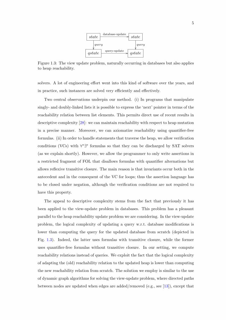
1.3 The view update problem, naturally occurring in databases but also
applies to heap reachability. . . . . . . . . . . . . . . . . . . . . . . . . . 5
1.4 The effect of an assignment statement on the heap viewed as a directed
graph. . . . . . . . . . . . . . . . . . . . . . . . . . . . . . . . . . . . . . 8
1.5 An example of a cutpoint into a linked list. . . . . . . . . . . . . . . . . 9
3.1 A simple Java program that reverses a list in-place. . . . . . . . . . . . . 26
3.2 Binary relation P as a directed graph. . . . . . . . . . . . . . . . . . . . 33
3.3 A simplified Java program that removes elements from a list according to
some predicate; for simplicity, we assume that the head is never removed. 39
3.4 Sample counterexample generated for a buggy version of insert for a
sorted list. Here, the loop invariant required that ∀α : (h〈n∗〉α ∧¬i〈n∗〉α) → α <val e (where <val is an ordering on nodes according to
their values), but the loop condition is true, therefore loop will execute
one more time, violating this. . . . . . . . . . . . . . . . . . . . . . . . 41
4.1 A procedure to insert the element pointed to by e into the non-empty,
(unsorted) singly-linked list pointed by h, just before the element x
(which must not be first). The while-loop uses the trailing-pointer idiom:
q is always one step behind p. . . . . . . . . . . . . . . . . . . . . . . . 45
5.1 Reversing a list pointed to by a head h with many shared nodes accessible
from outside the local heap (surrounded by a rounded rectangle). . . . . 65
xii
5.2 An annotated implementation of Union-Find in Java. f is the backbone
field denoting the parent of a tree node. . . . . . . . . . . . . . . . . . . 68
5.3 An example scenario of running find . . . . . . . . . . . . . . . . . . . . 69
5.4 An example scenario of running union. . . . . . . . . . . . . . . . . . . . 69
5.5 A case where changes made by find have a non-local effect. . . . . . . . 70
5.6 . . . . . . . . . . . . . . . . . . . . . . . . . . . . . . . . . . . . . . . . . 71
5.7 Memory states with non-unique pointers where global reasoning about
reachability is hard. . . . . . . . . . . . . . . . . . . . . . . . . . . . . . 72
5.8 The function enmod maps every node σ to the first node in mod reachable
from σ. Notice that for any α ∈ mod, enmod(α) = α by definition. . . . 74
5.9 Construction of a modified path from three segments . . . . . . . . . . . 74
5.10 A simple function that swaps two adjacent elements following x in a
singly-linked list. Dotted lines denote the new state after the swap. The
notation e.g. Ef (x, f1x) denotes the single edge from x to f1x following
the f field. . . . . . . . . . . . . . . . . . . . . . . . . . . . . . . . . . . 75
5.11 A subtle situation occurs when the path from σ passes through multiple
exit-points. In such a case, the relevant exit-point for σ〈f∗〉τ1 is t1,
whereas for σ〈f∗〉τ2 and τ1〈f∗〉τ2 it would be t2. . . . . . . . . . . . . . 76
5.12 An example of a procedure where the mod-set is not (essentially) convex. 76
5.13 Paths that go entirely untouched. enmod(σ1) = α, whereas enmod(σ2) =
null. . . . . . . . . . . . . . . . . . . . . . . . . . . . . . . . . . . . . . . 77
5.14 Specification of proc with placeholders. . . . . . . . . . . . . . . . . . . . 82
5.15 An example invocation of find inside union. . . . . . . . . . . . . . . . 83
5.16 The inner enmod is constructed from the outer one by composing with
an auxiliary function enB|A. . . . . . . . . . . . . . . . . . . . . . . . . . 84
6.1 A simple Java program that creates two correlated lists. . . . . . . . . . 91
6.2 A program that flattens a hierarchical structure of lists into a single
cyclic list. . . . . . . . . . . . . . . . . . . . . . . . . . . . . . . . . . . . 94


Chapter 1
Introduction
This thesis develops means for automated reasoning for the purpose of proving the
correctness of computer programs making excessive use of pointers. These include
programs manipulating linked data structures, such as linked lists, doubly-linked lists,
nested lists, and reverse trees. For automation we use industry-standard tools whose
efficiency has been proven in practice. The proposed logical frameworks reduces verifi-
cation problems into logical queries. We show that the set of queries thus generated is
a decidable one, so a definite answer (“yes” or “no”) is guaranteed.
The problem of software verification is about as old as software, perhaps even older.
Floyd and Hoare [19, 29] proposed logical frameworks to construct correctness proofs for
programs with respect to formal specifications—full correctness proofs, which contain
a proof for the program’s termination on its designated set of input, as well as the
adherence of its behavior to the one registered in the specification; and the more popular
partial correctness proofs, which relax the termination requirement. A continued effort
to mechanize the construction of such proofs existed ever since. Cousot and Cousot [10]
brought the advancement of abstract interpretation, providing a multitude of techniques
used to analyze software in various domains. Simple abstract interpretation techniques
are employed day-to-day by compilers due to their elegance, ease of implementation,
and good performance. Naturally, there is a trade-off between resource usage and
accuracy of the analysis; as a consequence such analyses, which are based on simple
abstractions, mostly provide approximate results.
Within the problem space of software verification, a particularly interesting subset
of programs is those making heavy use of pointers. In C and the C-style programming
languages that emerged as a result of its success, pointers are basic working tools
1
2 CHAPTER 1. INTRODUCTION
just like arithmetic operators and control structures, combining expressivity and low-
level efficiency. Separation logic, mostly due to Reynolds [55] and O’Hearn [35, 50],
has evolved to address this challenging aspect of programming. Challenges arise, by-
and-large, by the occurrence of aliasing in pointer programs: the situation where two
pointers contain the same address, hence a change in data stores at that address is
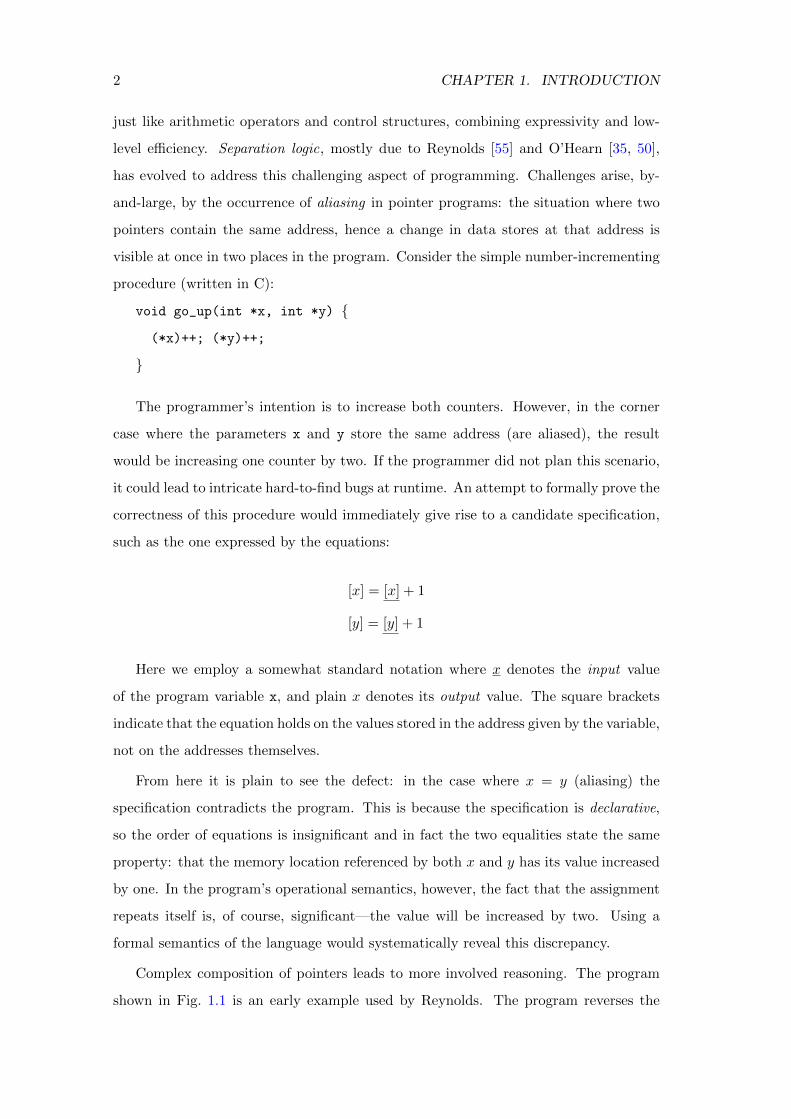
visible at once in two places in the program. Consider the simple number-incrementing
procedure (written in C):
void go_up(int *x, int *y) {(*x)++; (*y)++;
}
The programmer’s intention is to increase both counters. However, in the corner
case where the parameters x and y store the same address (are aliased), the result
would be increasing one counter by two. If the programmer did not plan this scenario,
it could lead to intricate hard-to-find bugs at runtime. An attempt to formally prove the
correctness of this procedure would immediately give rise to a candidate specification,
such as the one expressed by the equations:
[x] = [x] + 1
[y] = [y] + 1
Here we employ a somewhat standard notation where x denotes the input value
of the program variable x, and plain x denotes its output value. The square brackets
indicate that the equation holds on the values stored in the address given by the variable,
not on the addresses themselves.
From here it is plain to see the defect: in the case where x = y (aliasing) the
specification contradicts the program. This is because the specification is declarative,
so the order of equations is insignificant and in fact the two equalities state the same
property: that the memory location referenced by both x and y has its value increased
by one. In the program’s operational semantics, however, the fact that the assignment
repeats itself is, of course, significant—the value will be increased by two. Using a
formal semantics of the language would systematically reveal this discrepancy.
Complex composition of pointers leads to more involved reasoning. The program
shown in Fig. 1.1 is an early example used by Reynolds. The program reverses the

3
j := null ; while i 6= null do
(k := i.next ; i.next := j ; j := i ; i := k)
Figure 1.1: A classical program that performs in-place reversal of a list, adaptedfrom [55]
1i 2 3 4 5
1 2
j
3
i
4 5
1 2 3 4 5 j
(i)
(ii)
(iii)
Figure 1.2: The state of the memory during the execution of the list reversal program:(i) initial state; (ii) an intermediate state; (iii) final state.
order of elements in a linked list: its input is a linked list whose head is pointed to
by i and each node contains a field next holding a pointer to the next node (or null
to signify the last node). The program outputs a list of the same structure, only that
the elements occur in reversed order. The reversal is done in-place, so that the original
input list is overwritten by the output.
Reynolds identified an acute problem when reasoning with programs that traverse
such recursive data structures: the pointer i serving as the iterator is advanced at
each step, and the number of steps is not bounded. Therefore there is always a risk
that a value written on one iteration will be overwritten in subsequent iterations. In
particular, to make sure that the list remains acyclic in this example, one must obtain
that there is no next-path from j to i, otherwise the addition of the edge 〈i, j〉 introduces
a cycle.
We approach this problem by a careful construction of appropriate loop invariants
for iterative programs, and comprehensive summaries for recursive programs. Observ-
ing a typical run of reverse (Fig. 1.2), an important property of it can be noticed: the
pointer variables i and j always point into the beginning of two disjoint list segments.
Either segment may be empty (as in (i) and (iii)), but the segments never share el-
ements. It turns out that this property is crucial to prove the correctness of the list
reversal program. Formulating this property in logic is more involved than the previ-
ous, simpler aliasing conditions. To address this issue, we define reachability logics and
4 CHAPTER 1. INTRODUCTION
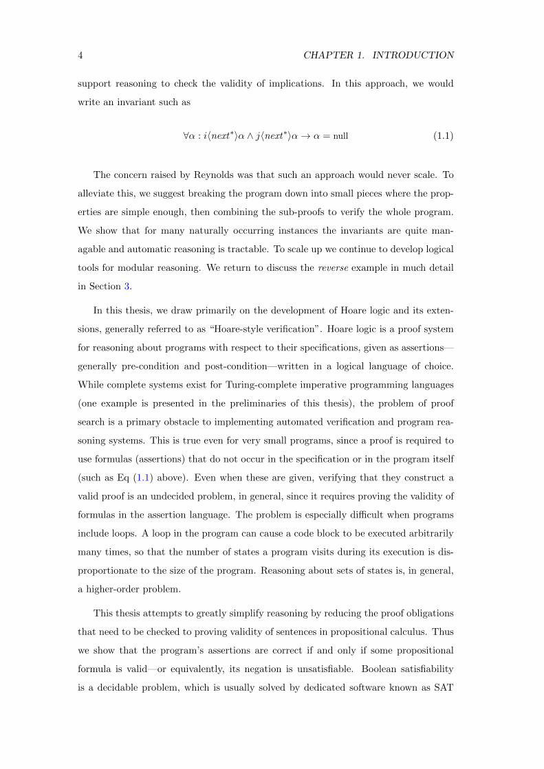
support reasoning to check the validity of implications. In this approach, we would
write an invariant such as
∀α : i〈next∗〉α ∧ j〈next∗〉α→ α = null (1.1)
The concern raised by Reynolds was that such an approach would never scale. To
alleviate this, we suggest breaking the program down into small pieces where the prop-
erties are simple enough, then combining the sub-proofs to verify the whole program.
We show that for many naturally occurring instances the invariants are quite man-
agable and automatic reasoning is tractable. To scale up we continue to develop logical
tools for modular reasoning. We return to discuss the reverse example in much detail
in Section 3.
In this thesis, we draw primarily on the development of Hoare logic and its exten-
sions, generally referred to as “Hoare-style verification”. Hoare logic is a proof system
for reasoning about programs with respect to their specifications, given as assertions—
generally pre-condition and post-condition—written in a logical language of choice.
While complete systems exist for Turing-complete imperative programming languages
(one example is presented in the preliminaries of this thesis), the problem of proof
search is a primary obstacle to implementing automated verification and program rea-
soning systems. This is true even for very small programs, since a proof is required to
use formulas (assertions) that do not occur in the specification or in the program itself
(such as Eq (1.1) above). Even when these are given, verifying that they construct a
valid proof is an undecided problem, in general, since it requires proving the validity of
formulas in the assertion language. The problem is especially difficult when programs
include loops. A loop in the program can cause a code block to be executed arbitrarily
many times, so that the number of states a program visits during its execution is dis-
proportionate to the size of the program. Reasoning about sets of states is, in general,
a higher-order problem.
This thesis attempts to greatly simplify reasoning by reducing the proof obligations
that need to be checked to proving validity of sentences in propositional calculus. Thus
we show that the program’s assertions are correct if and only if some propositional
formula is valid—or equivalently, its negation is unsatisfiable. Boolean satisfiability
is a decidable problem, which is usually solved by dedicated software known as SAT
5
statedatabase-update //
query
��
state
query
��qstate
query-update // qstate
Figure 1.3: The view update problem, naturally occurring in databases but also appliesto heap reachability.
solvers. A lot of engineering effort went into this kind of software over the years, and
in practice, such instances are solved very efficiently and effectively.
Two central observations underpin our method. (i) In programs that manipulate
singly- and doubly-linked lists it is possible to express the ‘next’ pointer in terms of the
reachability relation between list elements. This permits direct use of recent results in
descriptive complexity [28]: we can maintain reachability with respect to heap mutation
in a precise manner. Moreover, we can axiomatize reachability using quantifier-free
formulas. (ii) In order to handle statements that traverse the heap, we allow verification
conditions (VCs) with ∀∗∃∗ formulas so that they can be discharged by SAT solvers
(as we explain shortly). However, we allow the programmer to only write assertions in
a restricted fragment of FOL that disallows formulas with quantifier alternations but
allows reflexive transitive closure. The main reason is that invariants occur both in the
antecedent and in the consequent of the VC for loops; thus the assertion language has
to be closed under negation, although the verification conditions are not required to
have this property.
The appeal to descriptive complexity stems from the fact that previously it has
been applied to the view-update problem in databases. This problem has a pleasant
parallel to the heap reachability update problem we are considering. In the view-update
problem, the logical complexity of updating a query w.r.t. database modifications is
lower than computing the query for the updated database from scratch (depicted in
Fig. 1.3). Indeed, the latter uses formulas with transitive closure, while the former
uses quantifier-free formulas without transitive closure. In our setting, we compute
reachability relations instead of queries. We exploit the fact that the logical complexity
of adapting the (old) reachability relation to the updated heap is lower than computing
the new reachability relation from scratch. The solution we employ is similar to the use
of dynamic graph algorithms for solving the view-update problem, where directed paths
between nodes are updated when edges are added/removed (e.g., see [13]), except that

6 CHAPTER 1. INTRODUCTION
our solution is geared towards verification of heap-manipulating programs with linked
data structures.
Another aspect that complicates programmatic reasoning, especially with complex
states as is the case when pointer-based data structures are present, is procedures.
Programs are usually factored into several sub-programs in the interest of readability
and code reuse. This common idiom causes one code block to be executed in different
contexts, and it is highly desirable for reasons of scalability not to have to verify it
for each context separately. The challenge is to be able to express the view-update
that summarizes the effect of a procedure call in an arbitrary context, where some
of the elements are not reachable by the procedure, and therefore essentially remain
unmodified. This may be seen as an instance of the frame problem.
The rest of this thesis introduces reachability logics, a formal definition of logical
fragments found useful for the systematic reasoning over programs containing pointer
structures. As a primary technique, the semantics of such logics are embedded in
first-order logic for the use of automated solvers. While a severe limitation on the
expressivity of the defined logic, automated proof techniques prove to be so effective
compared to manual proofs, even for small, seemingly-obvious examples, that there is
much benefit to using them whenever possible.
The results in this thesis were published in [36], [38], and [37].
1.1 Main Results
1.1.1 Deterministic Transitive Closure
A key to the reasoning techniques presented in this thesis is the concept of deterministic
transitive closure and its introduction into first-order logic. We begin by defining the
notation 〈next∗〉, which denotes the reflexive transitive closure of a unary function
symbol next . The semantics are that x〈next∗〉y is true iff there is a sequence of
successive applications next to x that results in y (next(next(· · ·x · · · )) = y). The
restriction that transitive closure can only be applied to functions is what makes it
deterministic. As we will see, this form of transitive closure is much simpler to handle.
This has been noticed before, in other contexts, e.g. in [34].
It is then shown that 〈next∗〉 can be axiomatized in pure first-order logic, in the
same way that first-order logic with equality can be axiomatized in first-order logic
1.1. MAIN RESULTS 7
(without equality) by adding the equality axioms. One important restriction, however,
is that once the transitive closure is introduced, the original function cannot be used in
logical terms anymore— because the relationship between next and next∗ is not first-
order-expressible. While this seems severe, it turns out that many useful properties
of linked lists and some other linked data structures can be expressed this way. It
is analogous to reasoning about natural numbers without using succ (the successor
function) but with the relation ≤. In fact, it is easy to see that using quantification
one can define succ in terms of ≤:
succ(x) = y ⇔ ∀α : (x ≤ α ∧ α 6= x)↔ y ≤ α (1.2)
This leads to a second restriction: the axiomatization of 〈next∗〉 that we construct in
Section 3.2 is complete, but only for finite structures; hence, it is essential that the logic
used for reasoning has the finite model property : if a formula in the logic has a model,
then it also has a finite model. This is not true in general, of course, for first-order
formulas. One fragment of first-order logic that does have this property will receive
a lot of attention throughout this thesis is the Bernays-Schonfinkel-Ramsey class—
also referred to as effectively propositional (EPR). It is characterized by a relational
vocabulary, that is, only relation symbols and constants may occur in the signature
and no non-nullary function symbols, and a quantifier prefix limited to ∃∗∀∗ so that all
existential quantifiers precede the universal ones. Again, we show a range of benchmarks
demonstrating specifications that fall well within this restriction. In fact, most of the
time, just universal formulas suffice to express desired properties.
In particular, it is very important to be able to express in a precise manner the
effect of heap mutations performed by the program. A commonly used solution is to
model the heap as a long array of pointers and to use McCarthy’s axioms defining
the update of an array a at index i to the value e as a{i ← e}. However, the use of
transitive closure will lead us to expressions of the form 〈(next{i← e})∗〉, which cannot
be handled using the decidable logical fragment that we are interested in.
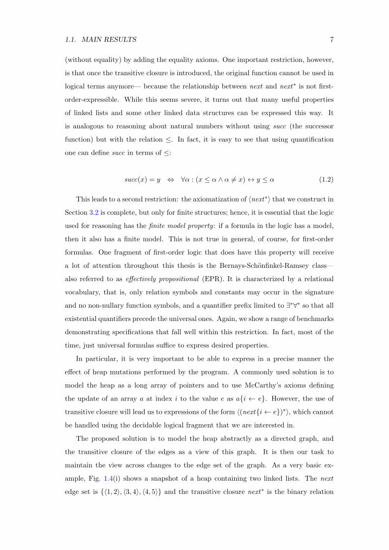
The proposed solution is to model the heap abstractly as a directed graph, and
the transitive closure of the edges as a view of this graph. It is then our task to
maintain the view across changes to the edge set of the graph. As a very basic ex-
ample, Fig. 1.4(i) shows a snapshot of a heap containing two linked lists. The next
edge set is {〈1, 2〉, 〈3, 4〉, 〈4, 5〉} and the transitive closure next∗ is the binary relation

8 CHAPTER 1. INTRODUCTION
1 2
i
3
j
4 5
1 2
i
3
j
4 5
(i)
(ii)
i.next := j
Figure 1.4: The effect of an assignment statement on the heap viewed as a directedgraph.
{〈1, 2〉, 〈3, 4〉, 〈3, 5〉, 〈4, 5〉}. The depicted assignment statement i.n := j causes the in-
sertion of a new edge 〈2, 3〉, which materializes many new paths in the view of next∗,
in particular: 〈1, 3〉, 〈1, 4〉, 〈1, 5〉, 〈2, 3〉, 〈2, 4〉, 〈2, 5〉 (as shown in Fig. 1.4(ii)); that is, all
the pairs where the first element belongs to the first list 1→ 2 and the second element
belongs to the second list 3→ 4→ 5. This can be formulated in logic as a view update:
α〈next∗〉β := α〈next∗〉β ∨(α〈next∗〉i ∧ j〈next∗〉β
)(1.3)
This shows that next∗ can be updated using only previous values of next∗. More-
over, this particular update is quantifier-free, which plays well with the quantifier prefix
limitations of EPR explained before. Chapter 3 and Chapter 5 extensively investigate
the capability to express various kinds of view updates in a logic with restricted vocab-
ulary and quantifiers.
1.1.2 Idempotent Functions in EPR
The use of EPR strictly rules out any function symbols other than constants. As a
corollary, we point out an interesting case where the use of a function is benign—in the
case where there is only one function symbol, and this function is idempotent , that is,
it is deducible from the axioms that ∀α : f(f(α)) = f(α). In this case we show that
there is a reduction from the satisfiability problem of formulas in the language that
includes f to satisfiability of EPR formulas without functions, but with the addition of
a finite number of constants and variables. The increase in formula size is linear in the
number of symbols used. Therefore, adding such a function symbol f does not break
the decidability property of the logical fragment. This extension can be used to write
formulas in a more natural way.

1.1. MAIN RESULTS 9
i
2 5 4 1 3
Figure 1.5: An example of a cutpoint into a linked list.
1.1.3 Procedural Reasoning with Adaptation
When dealing with a procedure that manipulates a linked-list segment or several linked-
list segments, the most difficult issue is the existence of cutpoints [56], which are pointers
from other areas of the heap that reach nodes of the list being manipulated. Such
pointers are represented in our abstraction of the heap as edges, which the procedure
does not modify and in fact may not even be able to observe, but may participate in
paths that are being connected or disconnected by it. As an example, assume that the
numbered list in Fig. 1.5 is being sorted by some sorting procedure. The node pointed
to by i is connected to the node 4 by a pointer field. Before the sorting, the set of nodes
reachable from i is, as seen in the figure, {4, 1, 3}. However, once the list is reordered
according to the numbering, the reachable set would become {4, 5}. This is despite the
fact that the sorting routine does not change i or the outgoing edge.
To support such reasoning, we define the notion of a mod-set , which is the area
of the heap being directly mutated by the procedure, and an entry function used to
describe the cutpoints by associating every “foreign” node from outside the mod-set
with the first location in the mod-set that is reachable from that node. This allows us to
formulate an adaptation rule that determines how the reachable set is modified for every
node outside the mod-set, essentially providing a complete, precise characterization of
the reachability relation 〈next∗〉 for the entire heap.
Having observed the behavior of several heap-manipulating procedures, we found
that they share a common desirable property: the amount of shared location introduced
by a single function call is bounded, and this bound can be known at compile time.
We take advantage of this property in order to produce modular verification conditions
that do not contain quantifier alternation, thus supporting our propositional reasoning
based on the small-model property.
We use the fact that the entry function is idempotent to support decidable reason-
ing using the adaptation rule within the scope of EPR as explained in the previous
10 CHAPTER 1. INTRODUCTION
paragraph. Thanks to this property, verification rules generated for the modular case
are still decidable for validity.
1.1.4 Template-based Verification with Induction
The downside of essentially every Floyd-Hoare verification technique is that it requires
analyzed programs to be annotated with a loop invariant for every loop that occurs in
the program. Furthermore, the supplied invariants should satisfy the restriction that
they are inductive, that is, any single loop iteration should preserve their validity by
induction: if invariant I holds at iteration k, we must be able to conclude that it holds
at iteration k+ 1 (if such an iteration exists, of course) without knowing anything else
about the state. This puts a heavy burden on a programmer who wishes to verify her
program using such a method, since the discovery of an appropriate inductive invariant
is usually not very intuitive. Furthermore, a small change in the program or in its
specifications may require considerable change in the loop invariant.
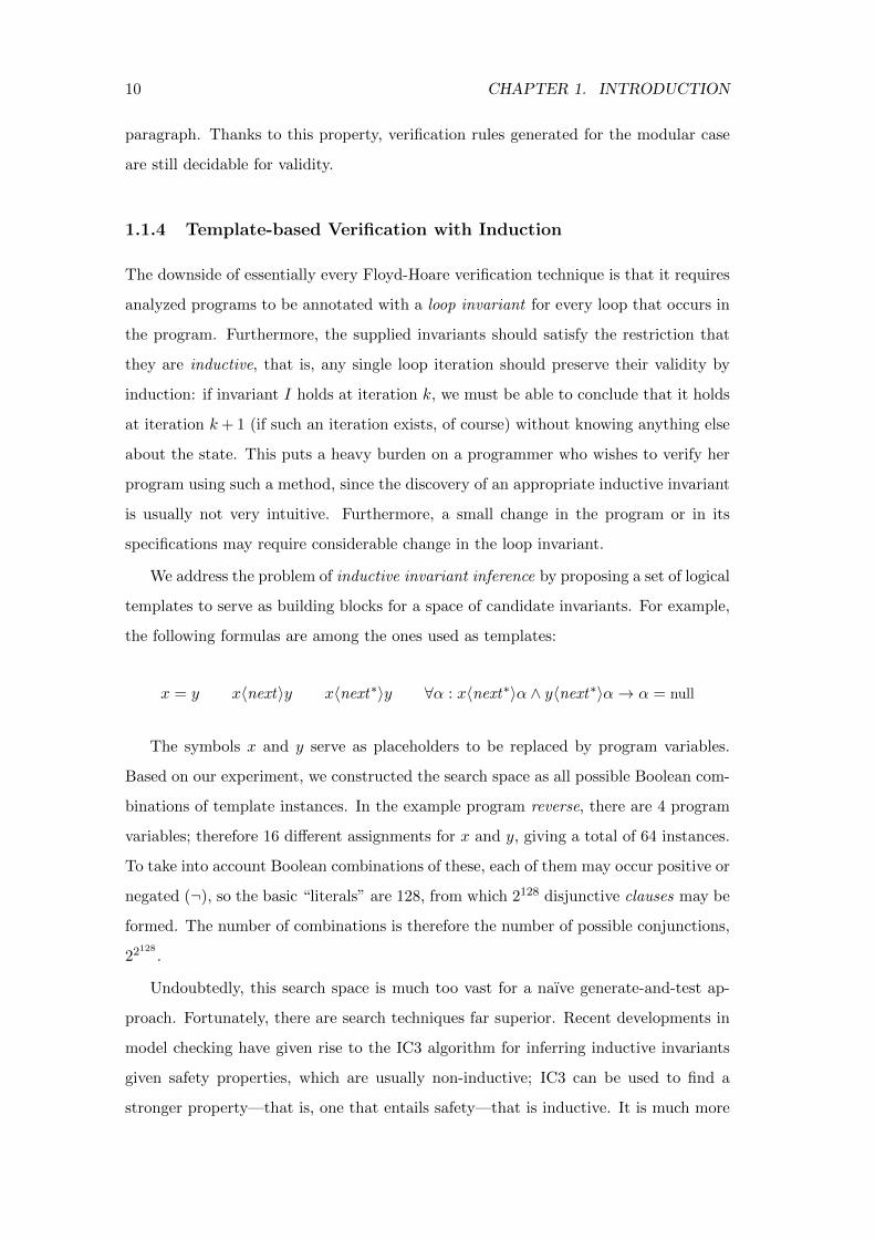
We address the problem of inductive invariant inference by proposing a set of logical
templates to serve as building blocks for a space of candidate invariants. For example,
the following formulas are among the ones used as templates:
x = y x〈next〉y x〈next∗〉y ∀α : x〈next∗〉α ∧ y〈next∗〉α→ α = null
The symbols x and y serve as placeholders to be replaced by program variables.
Based on our experiment, we constructed the search space as all possible Boolean com-
binations of template instances. In the example program reverse, there are 4 program
variables; therefore 16 different assignments for x and y, giving a total of 64 instances.
To take into account Boolean combinations of these, each of them may occur positive or
negated (¬), so the basic “literals” are 128, from which 2128 disjunctive clauses may be
formed. The number of combinations is therefore the number of possible conjunctions,
22128
.
Undoubtedly, this search space is much too vast for a naıve generate-and-test ap-
proach. Fortunately, there are search techniques far superior. Recent developments in
model checking have given rise to the IC3 algorithm for inferring inductive invariants
given safety properties, which are usually non-inductive; IC3 can be used to find a
stronger property—that is, one that entails safety—that is inductive. It is much more
1.1. MAIN RESULTS 11
efficient than an explicit exploration of the state space needed in order to discover all
the reachable states. Although originally developed to verify hardware systems, such
as Boolean circuits, where the state is represented as a string of bits of a known length,
we have found that it combines well with predicate abstraction, which allows to extend
its use to software systems with unbounded state resulting in infinitely many states.
We have effectively applied IC3 with predicate abstraction for the domain of linked-
list programs containing loops. The IC3 routine requires a theory solver, and the EPR-
based encoding of deterministic transitive closure makes a perfect match. To use it,
we made sure that all the abstraction predicates are expressible as universal formulas
in the language containing 〈next∗〉, and by careful construction of the two-vocabulary
formula ρ(X,X ′), where X is a set of “state symbols”, which are all the program
variables + the special symbol next∗, and X ′ are primed versions of all these symbols,
we obtained an instance of IC3 where all the satisfiability queries encountered during
its execution are of EPR formulas. This ensures termination and relative completeness
of the implementation. That is, if an inductive strengthening of the safety property
exists and is expressible as a Boolean combination of the abstraction predicates, the
algorithm is guaranteed to find it.
Consequently, we were able to automatically infer invariants for all the loops for
which we initially had to write inductive invariants manually. It should be noted that
invariants are restricted to a “weak” language, and that the results discovered by the
algorithm are very different than the ones a programmer would write naturally.
The above techniques proved effective for many naturally occurring programs. Suc-
cessful benchmarks include examples from the TVLA shape analysis framework [42]
using singly- and doubly-linked lists and nested lists, as well as some textbook al-
gorithm implementations: several sorting routines and the union-find data structure
developed by Tarjan [62].
Chapter 2
Preliminaries
2.1 Hoare-style Verification
Summary
• Computer programs represent transitions from an input state to an output state • Hoare logic
is a formal framework for reasoning about properties • Hoare triples define preconditions and
postconditions • Using proof rules, claims written as Hoare triples can be proven •
This section presents a formal proof system for proving properties of imperative pro-
grams, based on proof rules for individual language constructs. Historically R.W.Floyd
invented rules for reasoning about flow charts [19], and later C.A.R.Hoare modified and
extended these to treat programs written as code in an imperative programming lan-
guage [29]. To demonstrate this approach, consider a simplistic programming language
called “While-language” with the following abstract syntax:
a ::= n | X | a+ a | a− a | a× a
b ::= true | false | a = a | ¬b | b ∧ b | b ∨ b
c ::= skip | X := a | c; c | if b then c else c | while b do c
Here, n ranges over integer literals, and X ranges over program variables (occa-
sionally called locations). The syntactic group a represents arithmetic expressions; b
represents Boolean expressions; and c represents commands. We rely on the reader’s
intuitive model for understanding the behavior of programs written in While.
Definition 1 (Hoare triple). A partial correctness assertion (also referred to as a Hoare
12

2.1. HOARE-STYLE VERIFICATION 13
{A}skip{A} {Q[a/X]}X := a{Q}
{P}c1{C} {C}c2{Q}{P}c1; c2{Q}
{P ∧ [[B]]}c1{Q} {P ∧ ¬[[B]]}c2{Q}{P}if B then c1 else c2{Q}
{P ∧ [[B]]}c{P}{P}while B do c{P ∧ ¬[[B]]}
|= P → P ′ {P ′}c{Q′} |= Q′ → Q
{P}c{Q}
Table 2.1: Hoare rules for the basic While-language ([67]).
triple) has the form
{P} c {Q}
where c is a command and P , Q are assertions. We do not formally define the language
of assertions here, but assume they are written in some form of logic.
A partial correctness assertion is said to be valid (written |= {P} c {Q}) when every
successful computation of c from a state satisfying P results in a state satisfying Q.
For example,
|= {X > 3} X := X + 1 {X > 4}
Table 2.1 contains a set of inference rules for proving validity of partial correctness
assertions. The notation [[B]] is used for the semantics of a Boolean condition, expressed
as a logical formula. The proof rules are often called Hoare rules and the collection of
rules constitutes a proof system called Hoare logic.
The last rule (bottom right), called the consequence rule, is special because the
premises include validity of logical implications. Such implications may be hard to
prove for their own worth, and may require, for example, arithmetical reasoning. This
is the most complicated rule in the system, and is definitely required; indeed, without
it we would not even be able to prove some trivial assertion such as—
{X > 1} skip {X > 0}
Of course, this makes reasoning as hard as any logical reasoning in the logical
language of the assertions.
Proposition 1 (Soundness of Hoare logic). If an assertion {P}c{Q} is provable using
the proof system of Table 2.1, then |= {P}c{Q}.
14 CHAPTER 2. PRELIMINARIES
The proof of this proposition is carried out by systematic induction on the proof
tree. It is covered in detail in [67].
2.2 Completeness and Weakest-Precondition
Summary
• The weakest (liberal) precondition wlp is defined over a program c and a post-condition
formula Q • It is the weakest condition that must hold for an input state such that after
running c, the output state would satisfy Q • It was shown that wlp can be defined recursively
for many programming languages • This means that Hoare logic can prove any valid assertion,
given a complete proof system for the underlying assertion logic •
As Proposition 1 of the previous section shows, Hoare logic can only prove true
assertions. Is the converse also true—that every true assertion is provable in Hoare
logic? Clearly, this depends heavily on the nature of the assertion language: the logical
language used to describe P and Q. In particular, two important factors come into
play:
• Our ability to prove valid implications within the assertion logic; this is required
by the consequence rule.
• The capacity of the assertion language to express inductive loop invariants. This
is a subtle point and will be addressed later.
The completeness property of Hoare logic with respect to some assumed complete-
ness of the assertion language is known as relative completeness. To show it, we first
introduce a new concept.
Definition 2 (Weakest liberal precondition). The weakest liberal precondition of an
assertion Q with respect to a command c is defined as the set of states σ ∈ Σ where
every execution of c starting at state σ either diverges or terminates at a state σ′ such
that σ′ |= Q.
The term “liberal” refers to the possibility of divergence (non-termination) of c, and
is used to distinguish this term from a more strict variant where termination of c must

2.2. COMPLETENESS AND WEAKEST-PRECONDITION 15
wlp[[skip]](Q)def= Q
wlp[[x := a]](Q)def= Q[a/x]
wlp[[c1 ; c2]](Q)def= wlp[[c1]](wlp[[c2]](Q))
wlp[[if B then c1 else c2]](Q)def= [[B]] ∧ wlp[[c1]](Q) ∨¬[[B]] ∧ wlp[[c2]](Q)
wlp[[while B {I} do c]](Q)def= I
Table 2.2: Standard rules for computing weakest liberal preconditions for While-language procedures annotated with loop invariants and postconditions. I denotesthe loop invariant, [[B]] is the semantics of Boolean program conditions, and Q is thepostcondition — all are expressed as first-order formulas.
be preserved. In the remainder of the text, we omit the word “liberal” and just write
“weakest precondition”, but the intention is always “weakest liberal precondition”.
For the claim of relative completeness we would like to show that wlp[[c]](Q) is
expressible in the logical language of assertions. If the assertion language is closed
under Boolean connectives and syntactic substitution, and if the command c is loop-
free, then this is certainly the case, and explicit formulas for constructing it are given
in the first four lines of Table 2.2. Winskell [67] shows that for such c, it holds that
|= {P}c{Q} if and only if |= P → wlp[[c]]Q.
Inductive Loop Invariants
In the presence of loops, where the length of the program’s execution is not bounded,
the situation becomes more difficult, since these programs require reasoning on the
sets of reachable states from an arbitrary starting state—which may be infinite. This
usually requires the use of high-order logic. A common alternative is to require that
loops are annotated with an appropriate inductive loop invariant .
A loop invariant is a condition that holds at the beginning and at the end of
every loop iteration. An inductive loop invariant is a loop invariant with an additional
restriction: satisfaction of the invariant at iteration i of the loop (for i > 1) has to
follow solely from its satisfaction at iteration i− 1; it cannot be based on any previous
iterations.
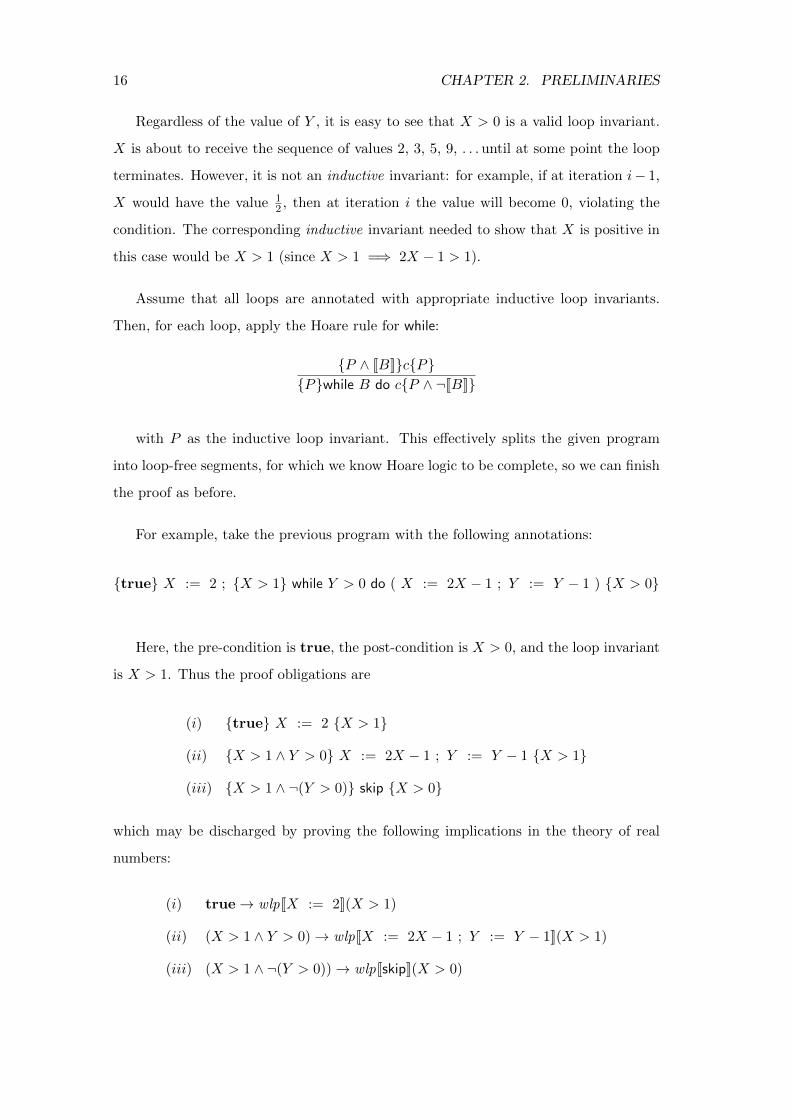
To illustrate this subtle, but crucial, difference, consider the example program:
X := 2 ; while Y > 0 do ( X := 2X − 1 ; Y := Y − 1 )
16 CHAPTER 2. PRELIMINARIES
Regardless of the value of Y , it is easy to see that X > 0 is a valid loop invariant.
X is about to receive the sequence of values 2, 3, 5, 9, . . . until at some point the loop
terminates. However, it is not an inductive invariant: for example, if at iteration i− 1,
X would have the value 12 , then at iteration i the value will become 0, violating the
condition. The corresponding inductive invariant needed to show that X is positive in
this case would be X > 1 (since X > 1 =⇒ 2X − 1 > 1).
Assume that all loops are annotated with appropriate inductive loop invariants.
Then, for each loop, apply the Hoare rule for while:
{P ∧ [[B]]}c{P}{P}while B do c{P ∧ ¬[[B]]}
with P as the inductive loop invariant. This effectively splits the given program
into loop-free segments, for which we know Hoare logic to be complete, so we can finish
the proof as before.
For example, take the previous program with the following annotations:
{true} X := 2 ; {X > 1} while Y > 0 do ( X := 2X − 1 ; Y := Y − 1 ) {X > 0}
Here, the pre-condition is true, the post-condition is X > 0, and the loop invariant
is X > 1. Thus the proof obligations are
(i) {true} X := 2 {X > 1}
(ii) {X > 1 ∧ Y > 0} X := 2X − 1 ; Y := Y − 1 {X > 1}
(iii) {X > 1 ∧ ¬(Y > 0)} skip {X > 0}
which may be discharged by proving the following implications in the theory of real
numbers:
(i) true→ wlp[[X := 2]](X > 1)
(ii) (X > 1 ∧ Y > 0)→ wlp[[X := 2X − 1 ; Y := Y − 1]](X > 1)
(iii) (X > 1 ∧ ¬(Y > 0))→ wlp[[skip]](X > 0)

2.3. DECIDABILITY 17
We can now state a completeness theorem for Hoare logic.
Theorem 1 (Hoare logic—completeness). Let c be a While-language command where
every loop is annotated with a loop invariant. If |= {P}c{Q} and, furthermore, all loop
invariants are valid and inductive, then there exists a Hoare proof for {P}c{Q}.
2.3 Decidability
Summary
• Transforming a Hoare triple into a formula also provides the other direction • If a logic has a
decision procedure for valid formulas, one can also decide the validity of a Hoare triple • Thus
effectively checking whether a program meets its specification • In many cases, you can get a
counterexample when the specification is violated • Examples of decidable logical languages
include Persburger arithmetic, real arithmetic, uninterpreted functions, and EPR •
Generating Verification Conditions Table 2.3 provides the standard rules for
computing first-order verification conditions corresponding to Hoare triples using weak-
est liberal preconditions. An auxiliary function VCaux is used for defining the set of
side conditions for the loops occurring in the program. These rules are standard and
their soundness and relative completeness have been discussed elsewhere (e.g. see [20]).
The rule for while loop is split into two parts: in the wlp we take just the loop
invariant, where VCaux asserts that loop invariants are inductive and implies the post-
condition for each loop.
Verification conditions allow to completely reduce checking the validity of (anno-
tated) partial correctness assertions to checking validity of logical formulas. To check
whether |= {P}c{Q} as a partial correctness assertion, under the assumption that
the inductive loop invariants have been chosen correctly, it is enough to verify that
|= VCgen({P}c{Q}) as a logical statement.
Remark. The rules may generate formulas of exponential size due to the extensive use
of syntactic substitution. Another solution can be implemented either by using a set
of symbols for every program point, or through the method of Flanagan and Saxe [18].
Such size optimization techniques are not discussed in this thesis.

18 CHAPTER 2. PRELIMINARIES
VCaux(S,Q)def= ∅ (for any atomic command S)
VCaux(S1;S2, Q)def= VCaux(S1,wlp[[S2]](Q)) ∪VCaux(S2, Q)
VCaux(if B then S1 else S2, Q)def= VCaux(S1, Q) ∪VCaux(S2, Q)
VCaux(while B {I} do S,Q)def= VCaux(S, I) ∪
{I ∧ [[B]]→ wlp[[S]](I), I ∧ ¬[[B]]→ Q}VCgen({P}S{Q}) def
=(P → wlp[[S]](Q)
)∧∧VCaux(S,Q)
Table 2.3: Standard rules for computing VCs using weakest liberal preconditions forprocedures annotated with loop invariants and pre/postconditions. The rules for com-puting wlp[[ ]] appear in Table 2.2. The auxiliary function VCaux accumulates a con-junction of VCs for the correctness of loops.
Of course, the problem of checking whether a Hoare triple is valid is undecidable
(for example, |= {true}c{false} iff c never terminates), so we can not hope to solve
it by reducing it to checking validity of logical formulas. Indeed, checking whether
a formula is valid is also undecidable in general; for first-order logic, the problem is
recursively enumerable (since one can enumerate all possible proofs and check them),
but not recursive. For first-order logic over finite structures, the problem is not even
r.e., and there is no complete proof system.
However, some subsets of logic are nicely behaved, in the sense that the problem
of checking whether a given formula is valid is decidable. Consequently, if one is able
to define a language with axiomatic semantics and corresponding wlp[[]] such that the
verification conditions are defined in such a logic, then the verification problem for
the set of programs expressible in that language becomes decidable by reduction to
checking of logical validity.
We give a few examples of decidable logics:
• Presburger arithmetic is the logic of natural numbers with only addition. The
language contains the constants 0 and 1, and the binary operator +, from which
all the natural numbers can be constructed. The only relation symbol is = for
equality. This is enough to express linear equations over natural numbers, as
multiplication by a natural constant can be expressed by successive applications
of +.
• Real arithmetic contains the real constants 0 and 1, equality, an order relation
≤, and the operations +, −, ·. It was shown by Tarski that the theory of real
closed fields can be axiomatized in first-order logic. Furthermore, this theory

2.4. EFFECTIVELY-PROPOSITIONAL LOGIC 19
admits quantifier elimination, so the problem is still decidable if the formulas
have quantifiers, even though the complexity becomes non-elementary.
• Quantifier-free with uninterpreted functions is the logic where languages are al-
lowed to contain any function and relation symbols, and where these symbols
may have any interpretation (in contrast with +, for example, which must be
interpreted as addition in all structures); the only designated symbol is = for
equality. Formulas must be quantifier-free and contain no variable symbols.
• Effectively-propositional logic is a subset of relational logic. It is introduced in
the next sub-section.
2.4 Effectively-propositional Logic
Summary
• Careful use of quantifiers leads to a decidable fragment of first-order logic • Avoid function
symbols and preserve a quantifier prefix of ∃∗∀∗ • For this family, it is known that satisfiablity
is reducable to Boolean SAT • Hence, it is also decidable • Despite the exponential complexity,
modern solvers solve it efficiently in practice •
In propositional logic, atomic formulas are just predicate symbols. When viewed as a
subset of first-order logic, it means that all predicates are nullary— take no arguments—
and therefore there are no terms: no function symbols, no variables, and no quantifiers.
The satisfiability problem for propositional formulas is widely known as SAT and is
NP-complete.
A slight extension would be to allow arbitrary arity of the predicates, and have
nullary function symbols (constants). Formulas are closed by nature and take the form
of a Boolean combination of shallow atoms such as:
ϕ = P (a)→ P (b) ∨Q(c, a)
It is easy to convince oneself that if this formula has a model, then it also has
one where a, b, and c are all different elements of the domain. This suggest that we
20 CHAPTER 2. PRELIMINARIES
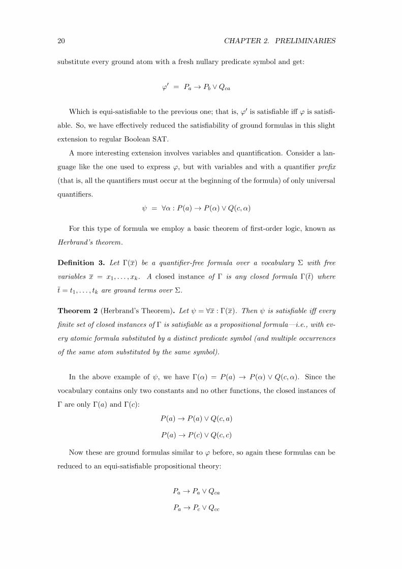
substitute every ground atom with a fresh nullary predicate symbol and get:
ϕ′ = Pa → Pb ∨Qca
Which is equi-satisfiable to the previous one; that is, ϕ′ is satisfiable iff ϕ is satisfi-
able. So, we have effectively reduced the satisfiability of ground formulas in this slight
extension to regular Boolean SAT.
A more interesting extension involves variables and quantification. Consider a lan-
guage like the one used to express ϕ, but with variables and with a quantifier prefix
(that is, all the quantifiers must occur at the beginning of the formula) of only universal
quantifiers.
ψ = ∀α : P (a)→ P (α) ∨Q(c, α)
For this type of formula we employ a basic theorem of first-order logic, known as
Herbrand’s theorem.
Definition 3. Let Γ(x) be a quantifier-free formula over a vocabulary Σ with free
variables x = x1, . . . , xk. A closed instance of Γ is any closed formula Γ(t) where
t = t1, . . . , tk are ground terms over Σ.
Theorem 2 (Herbrand’s Theorem). Let ψ = ∀x : Γ(x). Then ψ is satisfiable iff every
finite set of closed instances of Γ is satisfiable as a propositional formula—i.e., with ev-
ery atomic formula substituted by a distinct predicate symbol (and multiple occurrences
of the same atom substituted by the same symbol).
In the above example of ψ, we have Γ(α) = P (a) → P (α) ∨ Q(c, α). Since the
vocabulary contains only two constants and no other functions, the closed instances of
Γ are only Γ(a) and Γ(c):
P (a)→ P (a) ∨Q(c, a)
P (a)→ P (c) ∨Q(c, c)
Now these are ground formulas similar to ϕ before, so again these formulas can be
reduced to an equi-satisfiable propositional theory:
Pa → Pa ∨Qca
Pa → Pc ∨Qcc

2.4. EFFECTIVELY-PROPOSITIONAL LOGIC 21
Clearly this theory is satisfiable, e.g. by the assignment {P1, P2, Q1, Q2 7→ false}.This means that ψ is also satisfiable. To construct its model, we take the Herbrand
universe, which is the set of terms over the vocabulary Σ, in this case {a, c}, and make
it the domain; then we set the truth values of the predicates according to the satisfying
Boolean assignment:
P
a false
c false
Q a b
a X X
c false false
The X’s are “don’t-care” values, which may be either true or false.
Using Herbrand’s theorem, the satisfiability of every universal formula over a re-
lational vocabulary (with only predicate symbols, constants, and variables) reduces
to SAT. In fact, for any formula of the form ∃x∀y : Γ(x, y) we can apply first-order
Skolemization, introducing only new constants, because the existential variables x oc-
cur only on the outer level and are not nested inside universals. This means that the
vocabulary remains relational, and we can carry on with the reduction.
Definition 4 (EPR). Formulas of the form ∃x∀y : Γ(x, y) are called Effectively Propo-
sitional formulas.
The name comes from the fact that they can be simulated, as shown above, by a
propositional theory.
We should note that the size of the reduction is clearly exponential. The exponent
comes from the number of nested universal quantifiers in the formula, since every
universally quantified variable has to be instantiated with all possible constants. Hence,
if a large formula can be factored into many small formulas with a small degree of
nesting, this exponent can be reduced.
Logic with Equality
The reduction to SAT discusses only uninterpreted relation symbols. It is possible to
add a designated equality relation = by the usual technique of encoding the equality
22 CHAPTER 2. PRELIMINARIES
axioms:
∀α : α = α (reflexivity)
∀α, β : α = β → β = α (symmetry)
∀α, β, γ : α = β ∧ β = γ → α = γ (transitivity)
∀x1, x2 : x1 = x2 → P (x1)↔ P (x2)
for every predicate symbol P ∈ Σ
where x1, x2 are lists of distinct variables with length corresponding to the arity of P .
The formula x1 = x2 is a shorthand for a conjunction of pointwise equalities.
Since the theory of equality is relational and universal, it can be added to any
EPR formula and the reduction explained above would work just the same. The only
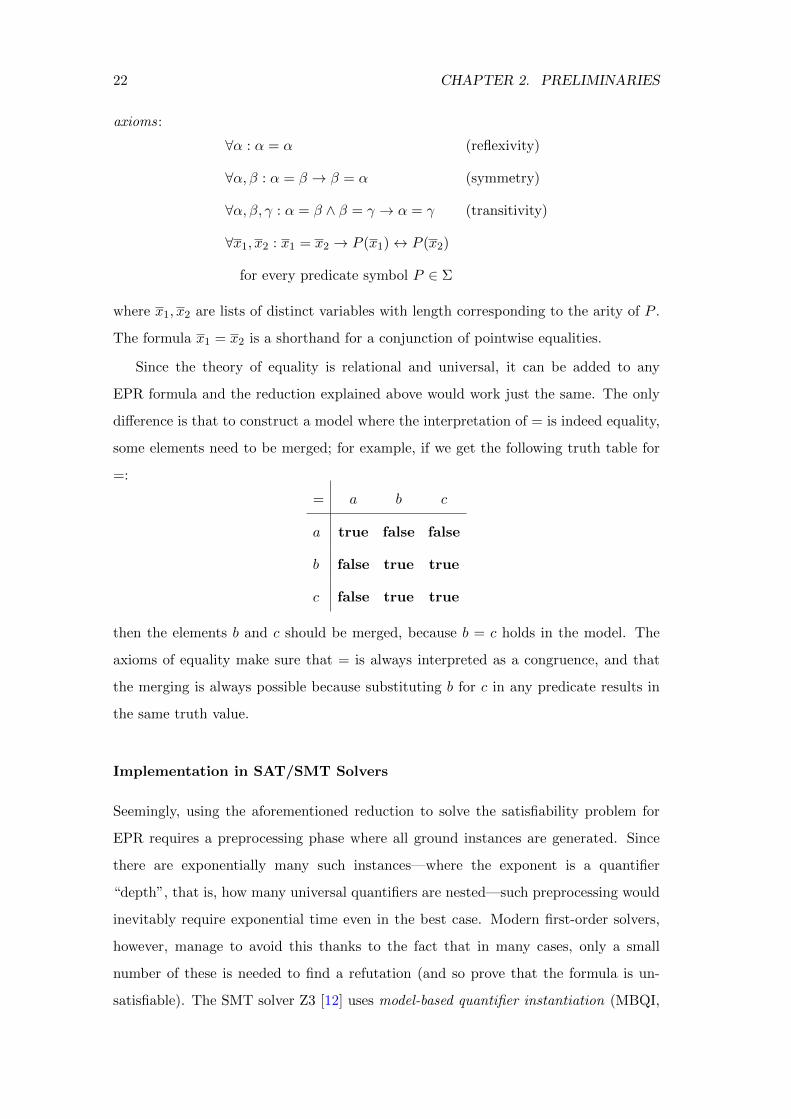
difference is that to construct a model where the interpretation of = is indeed equality,
some elements need to be merged; for example, if we get the following truth table for
=:
= a b c
a true false false
b false true true
c false true true
then the elements b and c should be merged, because b = c holds in the model. The
axioms of equality make sure that = is always interpreted as a congruence, and that
the merging is always possible because substituting b for c in any predicate results in
the same truth value.
Implementation in SAT/SMT Solvers
Seemingly, using the aforementioned reduction to solve the satisfiability problem for
EPR requires a preprocessing phase where all ground instances are generated. Since
there are exponentially many such instances—where the exponent is a quantifier
“depth”, that is, how many universal quantifiers are nested—such preprocessing would
inevitably require exponential time even in the best case. Modern first-order solvers,
however, manage to avoid this thanks to the fact that in many cases, only a small
number of these is needed to find a refutation (and so prove that the formula is un-
satisfiable). The SMT solver Z3 [12] uses model-based quantifier instantiation (MBQI,

2.4. EFFECTIVELY-PROPOSITIONAL LOGIC 23
explained e.g. in [23]) where variables in quantifiers are instantiated according to par-
tial candidate models for the input formula. This heuristic results in much less than
the exponential number of actual ground instances of the input formula, and leads to
very good running times in practice.
In the presence of an underlying theory, such as arithmetic or arrays, the power
of SMT (satisfiability modulo theory) solvers can be combined to solve even more
complicated formulas. Z3 also supports this form of reasoning.

Chapter 3
Pointer Manipulations
This chapter is based on the results published in [36].
3.1 Recursive Data Structures: The Need for Transitive
Closure
Summary
• The concept of pointers in data structures lends itself to first-order axiomatization • A pointer
field is thought of as a function mapping one object to another • Problems arise when the two
objects are of the same kind • The function can then be applied multiple types • Interesting
properties require reasoning about paths between objects, thus naturally requiring the use of
transitive closure •
Composite data structures are a desirable feature of a programming language. They
allow the programmer to reuse code by combining multiple entities and to define a hi-
erarchy of objects. For example, an object representing a book may contain a reference
to an object representing an author.
class Author {String firstName;
String lastName;
}
class Book {
24

3.1. RECURSIVE DATA STRUCTURES: THE NEED FOR TRANSITIVE CLOSURE25
String title;
Author author;
}
In this example, every Book instance is linked to at most one Author instance. The
heap space may then be described as two disjoint sets of objects, Book and Author ,
and a mathematical function author : Book → Author representing the pointer field.
In this case, if there are no more types defined, then a program having k variables of
type Author and m variables of type Book can manipulate at most k + 2m distinct
objects at any given time.
The situation becomes more complicated with the introduction of collections, which
require the use of recursive types. For example, a typical definition of a list looks like
the following:
class Node {String data;
Node next;
}
Fig. 3.1 presents a Java program for in situ reversal of a linked list. It is a type-safe
version of Fig. 1.1. Every node of the list has a next field that points to its successor
node in the list. Thus, we can model next as a function next : Node → Node that
maps a node in the list to its successor. Because we are going to use this function a
lot in this chapter and the following, we employ the abbreviation n for next in order
to keep formulas short and readable. Now, assume, for simplicity of the example, that
the program reverse manipulates the entire heap, that is, the heap consists of just the
nodes in the linked list, where the head of the input list is given as a formal parameter
h. To describe the heap that is reachable from h, we use the formula
∀α : h〈n∗〉α (3.1)
Where the special notation 〈n∗〉 means zero or more applications of n. In this case,
since the range of this function is the same as its domain, an unbounded number of

26 CHAPTER 3. POINTER MANIPULATIONS
Node reverse(Node h) {0: Node c = h;
1: Node d = null;
2: while 3: (c != null) {4: Node t = c.next;
5: c.next = null;
6: c.next = d;
7: d = c;
8: c = t;
}9: return d;
}
Figure 3.1: A simple Java program that reverses a list in-place.
I0def= ac ∧ ∀α : h〈n∗〉α
I3def= ac ∧ ∀α, β 6= null :
{α〈n∗〉β ⇔ β〈n∗0〉α d〈n∗〉αc〈n∗〉α ∧ (α〈n∗〉β ⇔ α〈n∗0〉β) ¬d〈n∗〉α
}I9 = ac ∧ ∀α : d〈n∗〉α ∧ (∀α, β : α〈n∗〉β ⇔ β〈n∗0〉α)
Table 3.1: AFR invariants for reverse (shown in Fig. 3.1). Note that n,n0 are functionsymbols while α〈n∗〉β, α〈n∗0〉β are atomic propositions on the reachability via directedpaths from α to β consisting of n, n0 edges.
elements can be accessed by repeated application — even for a program with only one
variable.
We also assume, for this chapter, that the heap is acyclic, i.e., the formula ac below
is a precondition of reverse.
acdef= ∀α, β : α〈n∗〉β ∧ β〈n∗〉α→ α = β (3.2)
Table 3.1 shows the invariants I0, I3 and I9 that describe a precondition, a loop
invariant, and a postcondition of reverse. They are expressed in AFR which permits use
of function symbols (e.g. n) in formulas only to express reachability (cf. n∗); moreover,
quantifier alternation is not permitted. The notation
f b
g ¬b
is shorthand for the
conditional (b ∧ f) ∨ (¬b ∧ g).
Note that I3 and I9 refer to n0, the value of n at procedure entry. The postcondi-
tion I9 says that reverse preserves acyclicity of the list and updates n so that, upon
procedure termination, the links of the original list have been reversed. It also says
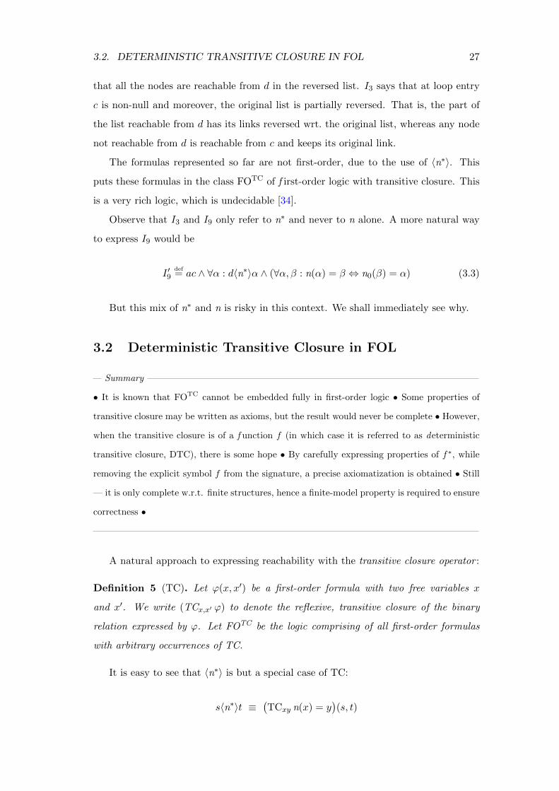
3.2. DETERMINISTIC TRANSITIVE CLOSURE IN FOL 27
that all the nodes are reachable from d in the reversed list. I3 says that at loop entry
c is non-null and moreover, the original list is partially reversed. That is, the part of
the list reachable from d has its links reversed wrt. the original list, whereas any node
not reachable from d is reachable from c and keeps its original link.
The formulas represented so far are not first-order, due to the use of 〈n∗〉. This
puts these formulas in the class FOTC of f irst-order logic with transitive closure. This
is a very rich logic, which is undecidable [34].
Observe that I3 and I9 only refer to n∗ and never to n alone. A more natural way
to express I9 would be
I ′9def= ac ∧ ∀α : d〈n∗〉α ∧ (∀α, β : n(α) = β ⇔ n0(β) = α) (3.3)
But this mix of n∗ and n is risky in this context. We shall immediately see why.
3.2 Deterministic Transitive Closure in FOL
Summary
• It is known that FOTC cannot be embedded fully in first-order logic • Some properties of
transitive closure may be written as axioms, but the result would never be complete • However,
when the transitive closure is of a f unction f (in which case it is referred to as deterministic
transitive closure, DTC), there is some hope • By carefully expressing properties of f∗, while
removing the explicit symbol f from the signature, a precise axiomatization is obtained • Still
— it is only complete w.r.t. finite structures, hence a finite-model property is required to ensure
correctness •
A natural approach to expressing reachability with the transitive closure operator :
Definition 5 (TC). Let ϕ(x, x′) be a first-order formula with two free variables x
and x′. We write (TCx,x′ ϕ) to denote the reflexive, transitive closure of the binary
relation expressed by ϕ. Let FOTC be the logic comprising of all first-order formulas
with arbitrary occurrences of TC.
It is easy to see that 〈n∗〉 is but a special case of TC:
s〈n∗〉t ≡(TCxy n(x) = y
)(s, t)

28 CHAPTER 3. POINTER MANIPULATIONS
FOTC is strictly more expressive than first-order logic. As a particular, fundamental
example, it is well-known that, according to the compactness theorem of first-order
logic, the set N of natural numbers is not first-order expressible. This means that
for every first-order theory whose theorems are valid over N, there must also be non-
standard models. Indeed, from the Lowenheim-Skolem theorem, it follows that it would
have models of any infinite cardinality. In contrast, the following FOTC theory [2]:
∀x : S(x) 6= 0
∀x, y : S(x) = S(y)→ x = y
∀x : (TCxy S(x) = y)(0, x)
∀x : x+ 0 = x
∀x : x+ S(y) = S(x+ y)
(3.4)
has only models that are isomorphic to N, where S is interpreted as the successor
function and + is interpreted as addition. Notice that (TCxy S(x) = y) evaluates to
≤, the less-than-or-equals relation. The axiomatization would not be complete if we
replaced it by the standard equivalent x ≤ y ⇔ ∃z : x+ z = y, which is first-order.
It has been shown, however, that adding TC, even with various restrictions of the
first-order language, leads immediately to an undecidable logic (that is, the satisfiabil-
ity/validity check for formulas in this language is undecidable); this can be shown by
reducing the satisfiability problem of universal FOTC formulas to tiling problems [33].
Attempts have been made to use first-order reasoning to mechanically prove prop-
erties of formulas with transitive closure. [44] suggests that we add the axiom
T1[f ] ≡ ∀u, v : ftc(u, v)↔ (u = v) ∨ ∃w : f(u,w) ∧ ftc(w, v)
Where ftc is a new binary relation symbol used to denote the transitive closure of
an existing binary relation whose symbol is f . While sound, it does not suffice to prove
many valid FOTC-theorems, and an induction principle is required, which goes beyond
first-order logic. This is not surprising, since FOTC could never be fully axiomatized
via a first-order theory.
We therefore try to find a fragment of FOTC that would be expressive enough to
describe interesting properties of pointer data structures, yet not too powerful as to

3.2. DETERMINISTIC TRANSITIVE CLOSURE IN FOL 29
become undecidable. As a first step to exploring the decidability of formulas containing
the transitive closure operator, we define names for several limited classes of formulas.
Definition 6. Let t1, t2, . . . tn be logical variables or constant symbols. We define four
types of atomic propositions:
1. true / false
2. t1 = t2 denoting equality
3. R(t1, t2, . . . , tr) denoting the application of relation symbol R of arity r
4. t1〈f∗〉t2 denoting the existence of k ≥ 0 such that fk(t1) = t2, where f0(t1)def= t1,
and fk+1(t1)def= f(fk(t1))
We say that t1〈f∗〉t2 is a reachability constraint between t1 and t2 via the func-
tion f .
• Quantifier-free formulas with Reachability (QFR) are Boolean combina-
tions of such formulas without quantifiers.
• Alternation-free formulas with Reachability (AFR) are Boolean combina-
tions of such formulas with additional quantifiers of the form ∀∗:ϕ or ∃∗:ϕ where
ϕ is a QFR formula.
• Forall-Exists Formulas with Reachability (AER) are Boolean combinations
of such formulas with additional quantifiers of the form ∀∗∃∗:ϕ where ϕ is a QFR
formula.
In particular, QFR ⊂ AFR ⊂ AER.
Inverting Reachability Constraints
A crucial step in moving from arbitrary FOTC formulas to AER or AFR formulas
is eliminating explicit uses of functions such as the “next” function, n. While this
may be difficult for a general graph, we show that it can be done for programs that
manipulate singly- and doubly-linked lists. In this section, we informally demonstrate
this elimination for acyclic lists. We observe that if n is acyclic, we can construct n+
from n∗ by
α〈n+〉β ⇔ α〈n∗〉β ∧ α 6= β (3.5)

30 CHAPTER 3. POINTER MANIPULATIONS
ΓlinOrddef= ∀α, β : n∗(α, β) ∧ n∗(β, α)↔ α = β ∧∀α, β, γ : n∗(α, β) ∧ n∗(β, γ)→ n∗(α, γ) ∧∀α, β, γ : n∗(α, β) ∧ n∗(α, γ)→ (n∗(β, γ) ∨ n∗(γ, β))
Table 3.2: ΓlinOrd says all points reachable from a given point are linearly ordered.
Also, since n is a function, the set of nodes reachable from a node α is totally
ordered by n∗. Therefore, n(α) is the minimal node in this order that is not α. The
minimality is expressed using extra universal quantification in
n(α) = β ⇔ α〈n+〉β ∧ ∀γ : α〈n+〉γ → β〈n∗〉γ (3.6)
This “inversion” shows that n can be expressed using AFR formulas. However,
caution must be practiced when using the elimination above, because it may introduce
unwanted quantifier alternations (see Section 6.1.1). Nevertheless our experiments
demonstrate that in a number of commonly occurring examples, the alternation can be
removed or otherwise avoided, yielding an equivalent AER/AFR formula.
Decidability of AER
Reachability constraints written as α〈n∗〉β are not directly expressible in FOL. How-
ever, AER formulas can be reduced to first-order ∀∗∃∗ formulas without function sym-
bols (which are decidable; see Section 2.4) in the following fashion: Introduce a new
binary relation symbol n∗ with the intended meaning that n∗(α, β) ↔ α〈n∗〉β. Even
though n∗ is an uninterpreted relation, we will consistently maintain the fact that it
models reachability. Every formula ϕ is translated into
ϕ′ def= ϕ[n∗(t1, t2)/t1〈n∗〉t2] (3.7)
For example, the acyclicity relation shown in Eq (3.2) is translated into:
acdef= ∀α, β : n∗(α, β) ∧ n∗(β, α)→ α = β (3.8)
We add the consistency rule ΓlinOrd shown in Table 3.2, which requires that n∗ is
a total order. This leads to the following propositions:
Proposition 2 (Simulation of AER). Consider an AER formula ϕ over vocabulary V =

3.2. DETERMINISTIC TRANSITIVE CLOSURE IN FOL 31
〈C, {n},R〉. Let ϕ′ def= ϕ[n∗(t1, t2)/t1〈n∗〉t2]. Then ϕ′ is a FO formula over vocabulary
V ′ = 〈C, ∅,R∪ {n∗}〉 and ϕ is simulated by ΓlinOrd → ϕ′ where ΓlinOrd is the formula
in Table 3.2.
By “simulate” we mean that the constructed first-order formula is valid iff the
given AER formula ϕ is valid. Appendix A.1 contains a proof of this proposition.
The proof constructs real models from “simulated” FO models using the reachability
inversion (Eq (3.6)).
Finite Model Property One thing to point out regarding the proof of Proposition 2,
is that it relies on the finiteness of the domain to reconstruct n from n∗. To illustrate,
consider the domain Q of rational numbers with the order ≤. This interpretation
satisfies all the properties due to ΓlinOrd, but for every two numbers x ≤ y, x 6= y,
there exists a number z such that x ≤ z ≤ y, z 6= x, z 6= y. In this case no element has
a successor, and we cannot use Eq (3.6) to reconstruct a function n such that n∗ = ≤.
This is the main reason for requiring the ∀∗∃∗ quantifier prefix for our formulas; without
it, not only does the logic become undecidable, but it is also not complete: not every
model of the “simulated” formula has a corresponding model of the original formula in
AER.
Expressivity of AER
Although Æ is a relatively weak logic, it can express interesting properties of lists. Typ-
ical predicates that express disjointness of two lists and sharing of tails are expressible
in Æ. For example, for two singly-linked lists with headers h, k, disjoint(h, k) ↔ ∀α :
α 6= null→ ¬(h〈n∗〉α ∧ k〈n∗〉α).
Another capability still within the power of Æ is to relax the earlier assumption
that the program manipulates the whole memory. We describe a summary of reverse
on arbitrary acyclic linked lists in a heap that may contain other linked data structures.
Realistic programs obey ownership requirements, e.g., the head h of the list owns the
input list which means that it is impossible to reach one of the list nodes without
passing through h. That is,
∀α, β : α 6= null→ (h〈n∗〉α ∧ β〈n∗〉α)→ h〈n∗〉β (3.9)

32 CHAPTER 3. POINTER MANIPULATIONS
This requirement is conjoined to the precondition, ac, of reverse. Its postcondition is
the conjunction of ac, the fact that h0 and d reach the same nodes, (i.e., ∀α : h0〈n∗0〉α↔d〈n∗〉α) and
∀α, β : α〈n∗〉β ↔
β〈n∗0〉α ∧ β 6= null h0〈n∗0〉α ∧ h0〈n∗0〉β
α〈n∗0〉β ¬h0〈n∗0〉α ∧ ¬h0〈n∗0〉β
false h0〈n∗0〉α ∧ ¬h0〈n∗0〉β
α〈n∗0〉h0 ∧ β = h0 ¬h0〈n∗0〉α ∧ h0〈n∗0〉β
(3.10)
Here, the bracketed formula should be read as a four-way case, i.e., as disjunction of
the formulas h0〈n∗0〉α ∧ h0〈n∗0〉β ∧ β〈n∗0〉α ∧ β 6= null; ¬h0〈n∗0〉α ∧ ¬h0〈n∗0〉β ∧ α〈n∗0〉β;
h0〈n∗0〉α∧¬h0〈n∗0〉β∧false; and, ¬h0〈n∗0〉α∧h0〈n∗0〉β∧α〈n∗0〉h0∧β = h0. Intuitively, this
summary distinguishes between the following four cases: (i) both the source (α) and the
target (β) are in the reversed list (ii) both source and target are outside of the reversed
list (iii) the source is in the reversed list and the target is not, and (iv) the source is
outside and the target is in the reversed list. Cases (i)–(iii) are self-explanatory. For
(iv) reachability can occur when there exists a path from α to h0 = β. Eq (3.10) is
a universal formula with 〈n∗0〉, so it is in AFR. In terms of [56], this means that we
assume that the procedure is cutpoint-free, that is, there are no pointers directly into
the middle of the list.
The more general case where arbitrary cutpoints occur requires more quantifiers. A
non-AFR formula also arises when we want to specify the behavior of this function in
this case (such an attempt is discussed in Section 6.1.2). We defer the issue of cutpoints
and handle it extensively in Section 5.
3.3 Updating Deterministic Transitive Closure
Summary
• The problem of view update is to maintain some view over a relation, while the underlying
relation changes • In context of TC, it means how paths change when edges are added or removed
• Recent results in descriptive complexity show that for DTC, the update is expressible in FOL
without quantifiers •
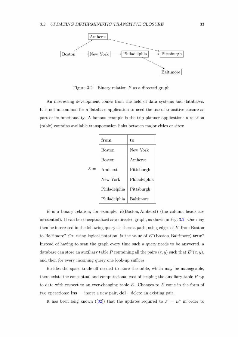
3.3. UPDATING DETERMINISTIC TRANSITIVE CLOSURE 33
Boston New York
Amherst
Philadelphia Pittsburgh
Baltimore
Figure 3.2: Binary relation P as a directed graph.
An interesting development comes from the field of data systems and databases.
It is not uncommon for a database application to need the use of transitive closure as
part of its functionality. A famous example is the trip planner application: a relation
(table) contains available transportation links between major cities or sites:
E =
from to
Boston New York
Boston Amherst
Amherst Pittsburgh
New York Philadelphia
Philadelphia Pittsburgh
Philadelphia Baltimore
E is a binary relation; for example, E(Boston,Amherst) (the column heads are
inessential). It can be conceptualized as a directed graph, as shown in Fig. 3.2. One may
then be interested in the following query: is there a path, using edges of E, from Boston
to Baltimore? Or, using logical notation, is the value of E∗(Boston,Baltimore) true?
Instead of having to scan the graph every time such a query needs to be answered, a
database can store an auxiliary table P containing all the pairs 〈x, y〉 such that E∗(x, y),
and then for every incoming query one look-up suffices.
Besides the space trade-off needed to store the table, which may be manageable,
there exists the conceptual and computational cost of keeping the auxiliary table P up
to date with respect to an ever-changing table E. Changes to E come in the form of
two operations: ins — insert a new pair, del – delete an existing pair.
It has been long known ([32]) that the updates required to P = E∗ in order to
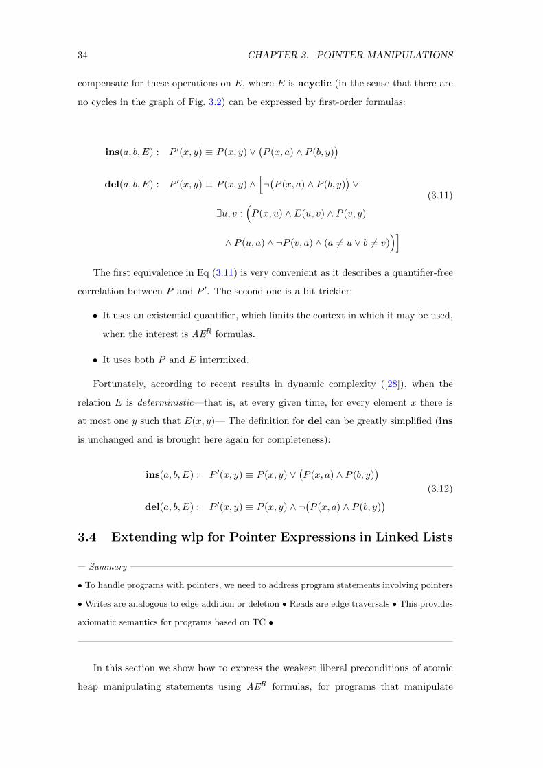
34 CHAPTER 3. POINTER MANIPULATIONS
compensate for these operations on E, where E is acyclic (in the sense that there are
no cycles in the graph of Fig. 3.2) can be expressed by first-order formulas:
ins(a, b, E) : P ′(x, y) ≡ P (x, y) ∨(P (x, a) ∧ P (b, y)
)del(a, b, E) : P ′(x, y) ≡ P (x, y) ∧
[¬(P (x, a) ∧ P (b, y)
)∨
∃u, v :(P (x, u) ∧ E(u, v) ∧ P (v, y)
∧ P (u, a) ∧ ¬P (v, a) ∧ (a 6= u ∨ b 6= v))]
(3.11)
The first equivalence in Eq (3.11) is very convenient as it describes a quantifier-free
correlation between P and P ′. The second one is a bit trickier:
• It uses an existential quantifier, which limits the context in which it may be used,
when the interest is AER formulas.
• It uses both P and E intermixed.
Fortunately, according to recent results in dynamic complexity ([28]), when the
relation E is deterministic—that is, at every given time, for every element x there is
at most one y such that E(x, y)— The definition for del can be greatly simplified (ins
is unchanged and is brought here again for completeness):
ins(a, b, E) : P ′(x, y) ≡ P (x, y) ∨(P (x, a) ∧ P (b, y)
)del(a, b, E) : P ′(x, y) ≡ P (x, y) ∧ ¬
(P (x, a) ∧ P (b, y)
) (3.12)
3.4 Extending wlp for Pointer Expressions in Linked Lists
Summary
• To handle programs with pointers, we need to address program statements involving pointers
•Writes are analogous to edge addition or deletion • Reads are edge traversals • This provides
axiomatic semantics for programs based on TC •
In this section we show how to express the weakest liberal preconditions of atomic
heap manipulating statements using AER formulas, for programs that manipulate
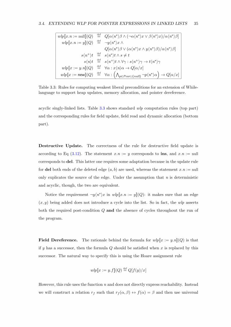
3.4. EXTENDING WLP FOR POINTER EXPRESSIONS IN LINKED LISTS 35
wlp[[x.n := null]](Q)def= Q[α〈n∗〉β ∧ (¬α〈n∗〉x ∨ β〈n∗〉x)/α〈n∗〉β]
wlp[[x.n := y]](Q)def= ¬y〈n∗〉x ∧
Q[α〈n∗〉β ∨ (α〈n∗〉x ∧ y〈n∗〉β)/α〈n∗〉β]
s〈n+〉t def= s〈n∗〉t ∧ s 6= t
s〈n〉t def= s〈n+〉t ∧ ∀γ : s〈n+〉γ → t〈n∗〉γ
wlp[[x := y.n]](Q)def= ∀α : x〈n〉α→ Q[α/x]
wlp[[x := new]](Q)def= ∀α :
(∧p∈Pvar∪{null} ¬p〈n∗〉α
)→ Q[α/x]
Table 3.3: Rules for computing weakest liberal preconditions for an extension of While-language to support heap updates, memory allocation, and pointer dereference.
acyclic singly-linked lists. Table 3.3 shows standard wlp computation rules (top part)
and the corresponding rules for field update, field read and dynamic allocation (bottom
part).
Destructive Update. The correctness of the rule for destructive field update is
according to Eq (3.12). The statement x.n := y corresponds to ins, and x.n := null
corresponds to del. This latter one requires some adaptation because in the update rule
for del both ends of the deleted edge (a, b) are used, whereas the statement x.n := null
only explicates the source of the edge. Under the assumption that n is deterministic
and acyclic, though, the two are equivalent.
Notice the requirement ¬y〈n∗〉x in wlp[[x.n := y]](Q): it makes sure that an edge
(x, y) being added does not introduce a cycle into the list. So in fact, the wlp asserts
both the required post-condition Q and the absence of cycles throughout the run of
the program.
Field Dereference. The rationale behind the formula for wlp[[x := y.n]](Q) is that
if y has a successor, then the formula Q should be satisfied when x is replaced by this
successor. The natural way to specify this is using the Hoare assignment rule
wlp[[x := y.f ]](Q)def= Q[f(y)/x]
However, this rule uses the function n and does not directly express reachability. Instead
we will construct a relation rf such that rf (α, β) ↔ f(α) = β and then use universal

36 CHAPTER 3. POINTER MANIPULATIONS
quantifications to “access” the value
wlp[[x := y.f ]](Q)def= ∀α : rf (y, α)→ Q[α/x]
Since, for regular singly-linked lists, n is acyclic, we do not need a symbol for rn —
we can express rn in terms of n∗ as follows. First we observe that n(α) 6= α. Also, since
n is a function, the set of nodes reachable from α is totally ordered by n∗. Therefore,
similarly to Eq (3.6), we can express rn(α, β) as the minimal node β in this order where
β 6= α. Expressing minimality “costs” one extra universal quantification.
In Table 3.3, formula s〈n〉t expresses rn(s, t) in terms of n∗: s〈n〉t holds if and only if
there is a path of length 1 between s and t (source and target). Thus, y〈n〉α is satisfied
exactly when α = n(y). If y does not have a successor, then y〈n〉α can only be true if
α = null, hence Q should be satisfied when x is replaced by null, which is in line with
the concrete semantics.
Lemma 3 in Appendix A.1 shows that the formula Pn correctly defines n as a
relation.
Dynamic allocation. The rule wlp[[x := new]](Q) expresses the semantic uncertainty
caused by the behavior of the memory allocator. We want to be compatible with any
run-time memory management, so we do not enforce a concrete allocation policy, but
instead require that the allocated node meets some reasonable specifications, namely,
that it is different from all values stored in program variables, and that it is unreachable
from any other node allocated previously (Note: for programs with explicit free(),
this assumption relies on the absence of dangling pointers, which can be verified by
introducing appropriate assertions; this is, however, beyond the scope of this thesis).
It should be noted that the rules for field dereference and for allocation admit an
additional level of quantifier nesting. As explained in Section 2.4, the number of nested
universal quantifiers in an EPR formula contributes an exponential component to the
complexity of solving it. This is usually not a scalability problem because the program
is broken down into its loop-free code segments, which are typically small. If there is
a long loop-free block, it can be broken down by (manually) adding assertions in the
middle of it.
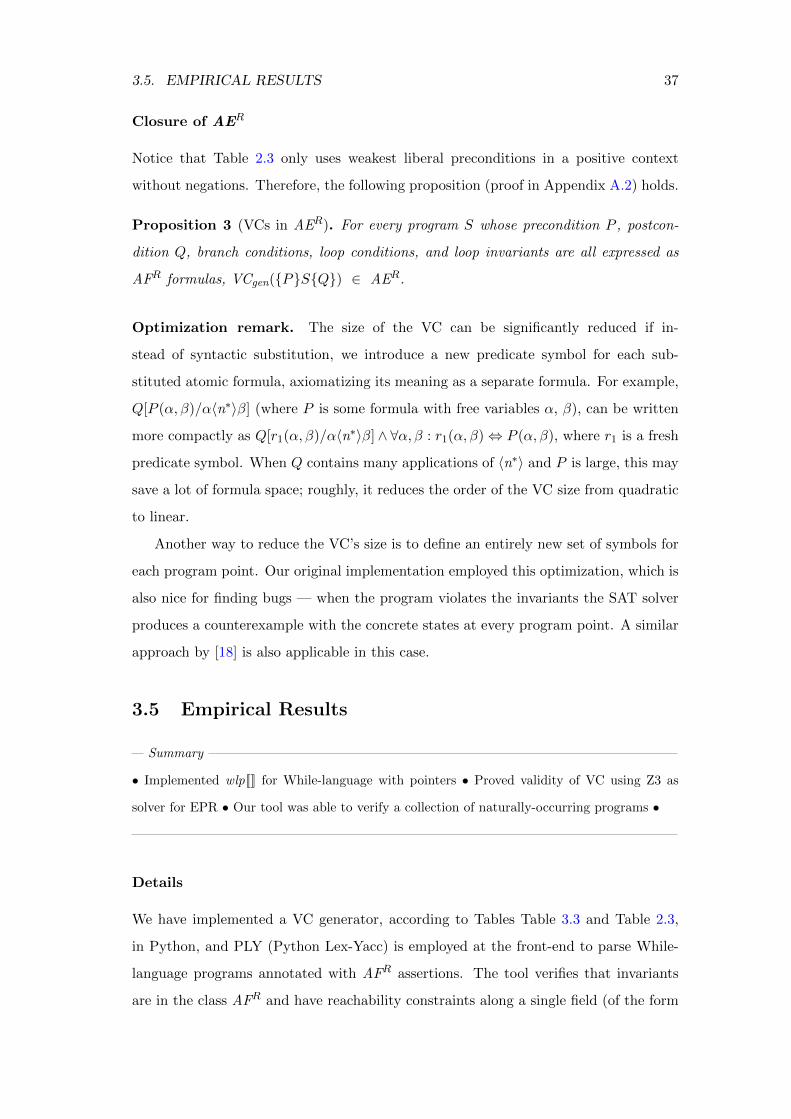
3.5. EMPIRICAL RESULTS 37
Closure of AER
Notice that Table 2.3 only uses weakest liberal preconditions in a positive context
without negations. Therefore, the following proposition (proof in Appendix A.2) holds.
Proposition 3 (VCs in AER). For every program S whose precondition P , postcon-
dition Q, branch conditions, loop conditions, and loop invariants are all expressed as
AFR formulas, VCgen({P}S{Q}) ∈ AER.
Optimization remark. The size of the VC can be significantly reduced if in-
stead of syntactic substitution, we introduce a new predicate symbol for each sub-
stituted atomic formula, axiomatizing its meaning as a separate formula. For example,
Q[P (α, β)/α〈n∗〉β] (where P is some formula with free variables α, β), can be written
more compactly as Q[r1(α, β)/α〈n∗〉β]∧ ∀α, β : r1(α, β)⇔ P (α, β), where r1 is a fresh
predicate symbol. When Q contains many applications of 〈n∗〉 and P is large, this may
save a lot of formula space; roughly, it reduces the order of the VC size from quadratic
to linear.
Another way to reduce the VC’s size is to define an entirely new set of symbols for
each program point. Our original implementation employed this optimization, which is
also nice for finding bugs — when the program violates the invariants the SAT solver
produces a counterexample with the concrete states at every program point. A similar
approach by [18] is also applicable in this case.
3.5 Empirical Results
Summary
• Implemented wlp[[]] for While-language with pointers • Proved validity of VC using Z3 as
solver for EPR • Our tool was able to verify a collection of naturally-occurring programs •
Details
We have implemented a VC generator, according to Tables Table 3.3 and Table 2.3,
in Python, and PLY (Python Lex-Yacc) is employed at the front-end to parse While-
language programs annotated with AFR assertions. The tool verifies that invariants
are in the class AFR and have reachability constraints along a single field (of the form

38 CHAPTER 3. POINTER MANIPULATIONS
f∗). The assertions may refer to the store and heap at the entry to the procedure via
x0, f0, etc. SMT-LIB v2 [5] standard notation is used to format the VC and to invoke
Z3. The validity of the VC can be checked by providing its negation to Z3. If Z3
exhibits a satisfying assignment then that serves as counterexample for the correctness
of the assertions. If no satisfying assignment exists, then the generated VC is valid,
and therefore the program satisfies the assertions.
The output model/counterexample (S-Expression), if one is generated, is then also
parsed, so that we have the truth table of n∗. This structure represents the state of the
program either at entry or at the beginning of a loop iteration: running the program
from this point will violate one or more invariants. To provide feedback to the user, n
is recovered by computing Eq (3.6), and then the pygraphviz tool is used to visualize
and present to the user a directed graph, whose vertices are nodes in the heap, and
whose edges are the n pointer fields.
We also implemented two procedures for generating VCs: the first one implements
the standard rules shown in Table 2.3 and a second one uses a separate set of (predicate
and constant) symbols per program point as a way to reduce the size of the generated
VC formula, as explained in the optimization remark above. We only report data on
the former since it exhibited shorter running times, through the latter may scale better.
Verification Examples
We have written AFR loop invariants and procedure pre- and postconditions for 13
example procedures shown in Table 3.5. These are standard benchmarks and what they
do can be inferred either from their names or from Table 3.4. We are encouraged by
the fact that it was not difficult to express assertions in AFR for these procedures. The
annotated examples and the VC generation tool are publicly available from bitbucket.
org/tausigplan/epr-verification.
For an example of the annotations used in the benchmarks, see Table 3.1, listing the
precondition, loop invariant, and postcondition of reverse. More examples are given in
Appendix B.
As expected, Z3 is able to verify all the correct programs. Table 3.5 shows statistics
for size and complexity of the invariants and the running times for Z3. The tests were
conducted on a 1.7GHz Intel Core i5 machine with 4GB of RAM, running OS X 10.7.5.
The version of Z3 used was 4.2, compiled for 64-bit Intel architecture (using gcc 4.2,
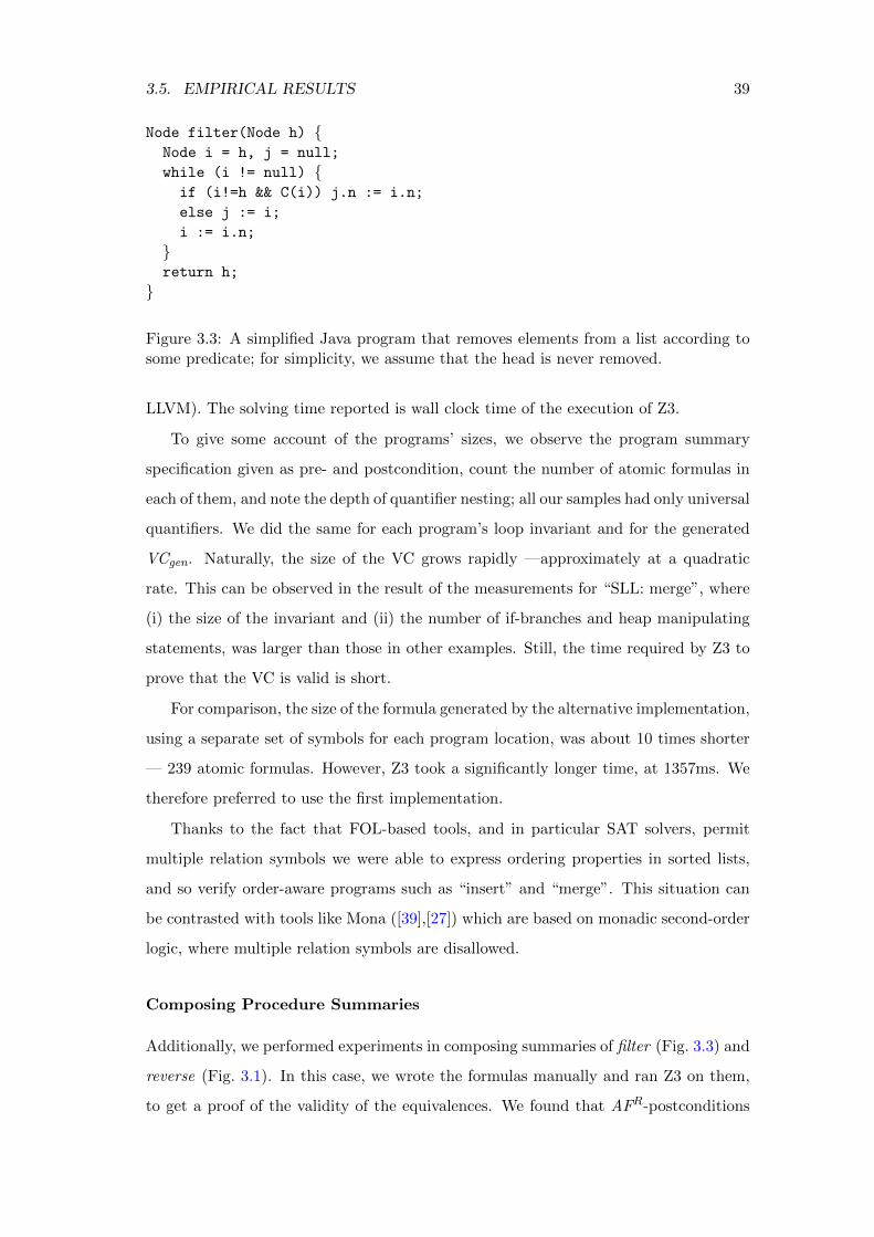
3.5. EMPIRICAL RESULTS 39
Node filter(Node h) {Node i = h, j = null;
while (i != null) {if (i!=h && C(i)) j.n := i.n;
else j := i;
i := i.n;
}return h;
}
Figure 3.3: A simplified Java program that removes elements from a list according tosome predicate; for simplicity, we assume that the head is never removed.
LLVM). The solving time reported is wall clock time of the execution of Z3.
To give some account of the programs’ sizes, we observe the program summary
specification given as pre- and postcondition, count the number of atomic formulas in
each of them, and note the depth of quantifier nesting; all our samples had only universal
quantifiers. We did the same for each program’s loop invariant and for the generated
VCgen. Naturally, the size of the VC grows rapidly —approximately at a quadratic
rate. This can be observed in the result of the measurements for “SLL: merge”, where
(i) the size of the invariant and (ii) the number of if-branches and heap manipulating
statements, was larger than those in other examples. Still, the time required by Z3 to
prove that the VC is valid is short.
For comparison, the size of the formula generated by the alternative implementation,
using a separate set of symbols for each program location, was about 10 times shorter
— 239 atomic formulas. However, Z3 took a significantly longer time, at 1357ms. We
therefore preferred to use the first implementation.
Thanks to the fact that FOL-based tools, and in particular SAT solvers, permit
multiple relation symbols we were able to express ordering properties in sorted lists,
and so verify order-aware programs such as “insert” and “merge”. This situation can
be contrasted with tools like Mona ([39],[27]) which are based on monadic second-order
logic, where multiple relation symbols are disallowed.
Composing Procedure Summaries
Additionally, we performed experiments in composing summaries of filter (Fig. 3.3) and
reverse (Fig. 3.1). In this case, we wrote the formulas manually and ran Z3 on them,
to get a proof of the validity of the equivalences. We found that AFR-postconditions
40 CHAPTER 3. POINTER MANIPULATIONS
of procedure summaries can be sequentially composed for this purpose.
Illustrating reverse(reverse h) = h. Let n∗1 denote the reachability after running
the inner reverse, and let n∗2 denote the reachability after running the outer reverse.
We can express the equivalence of reverse(reverse h) and h using the following AFR
implication:
(∀α, β : α〈n∗1〉β ⇔ β〈n∗0〉α) ∧ (∀α, β : α〈n∗2〉β ⇔ β〈n∗1〉α)
=⇒ ∀α, β : α〈n∗2〉β ⇔ α〈n∗0〉β(3.13)
The second conjunct of the implication’s antecedent describes the effect of the inner
reverse on the initial state while the third conjunct describes the effect of the outer
reverse on the state resulting from the first. The consequent of the implication states
that the initial and final states are equivalent.
Illustrating filter(C, reverse(h)) = reverse(filter(C, h)). The program filter takes a
unary predicate C on nodes, and a list with head h, and returns a list with all nodes
satisfying C removed. The postcondition of filter is: ∀α, β : α〈n∗〉β ⇔ ¬C(α)∧¬C(β)∧α〈n∗0〉β. It says that β is reachable from α in the filtered list provided neither α nor
β satisfies C and β was reachable from α initially. We show that the equivalence
of filter(C, reverse(h)) and reverse(filter(C, h)) can be expressed using an AFR-
theorem:
(∀α, β : α〈n∗1〉β ⇔ β〈n∗0〉α) ∧
(∀α, β : α〈n∗2〉β ⇔ ¬C(α) ∧ ¬C(β) ∧ α〈n∗1〉β) ∧
(∀α, β : α〈n∗1′〉β ⇔ ¬C(α) ∧ ¬C(β) ∧ α〈n∗0〉β) ∧
(∀α, β : α〈n∗2′〉β ⇔ β〈n∗1′〉α)
=⇒
∀α, β : α〈n∗2〉β ⇔ α〈n∗2′〉β
Here n∗1 denotes the reachability after running reverse on the input list (first conjunct
of the implication’s antecedent) and n∗2 denotes the reachability after running filter on
this reversed list (second conjunct). Similarly n∗1′ denotes the reachability after running
filter on the input list (third conjunct) and n∗2′ denotes the reachability after running

3.5. EMPIRICAL RESULTS 41
SLL: insert — Adds a node into a sorted list, preserving order.
SLL: find — Locates the first item in the list with a given value.
SLL: last — Returns the last node of the list.
SLL: merge — Merges two sorted lists into one, preserving order.
SLL: swap — Exchanges the first and second element of a list.
DLL: fix — Directs the back-pointer of each node towards the pre-vious node, as required by data structure invariants.
DLL: splice — Splits a list into two well-formed doubly-linked lists.
Table 3.4: Description of some linked list manipulating programs verified by our tool.
Node insert(Node h, Node e) {Node i = h, j = null;
while (i != null && e.val >= i.val) {j = i; i = i.n;
}if (j != null) { j.n = e; e.n = i; }else { e.n = h; h = e; }return h;
}
v v
v
n
ih
e
Figure 3.4: Sample counterexample generated for a buggy version of insert for asorted list. Here, the loop invariant required that ∀α : (h〈n∗〉α ∧ ¬i〈n∗〉α) → α <val e(where <val is an ordering on nodes according to their values), but the loop conditionis true, therefore loop will execute one more time, violating this.
reverse on this filtered list (fourth conjunct). The consequent of the implication states
that the reachability after performing the first execution path (first reverse, then fil-
ter) is equivalent to that after performing the second execution path (first filter, then
reverse).
Buggy Examples
We also applied the tool to erroneous programs and programs with incorrect assertions.
The results, including run-time statistics and formula sizes, are reported in Table 3.6.
In addition, we measured the size of the model generated, by observing the size of the
generated domain—which reflects the number of nodes in the heap. As expected, Z3
was able to produce a concrete counterexample of a small size. Since these are slight
variations of the correct programs, size and running time statistics are similar.
An example of generated output when a program fails to verify can be seen, for the
insert program, in Fig. 3.4. The tool reports, as part of its output, that a counterex-
ample occurs when j = null and h.val = i.val = e.val.
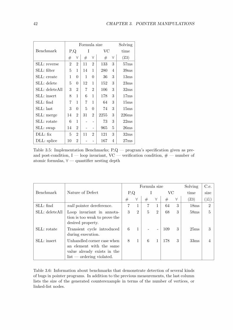
42 CHAPTER 3. POINTER MANIPULATIONS
Benchmark
Formula size Solving
P,Q I VC time
# ∀ # ∀ # ∀ (Z3)
SLL: reverse 2 2 11 2 133 3 57ms
SLL: filter 5 1 14 1 280 4 39ms
SLL: create 1 0 1 0 36 3 13ms
SLL: delete 5 0 12 1 152 3 23ms
SLL: deleteAll 3 2 7 2 106 3 32ms
SLL: insert 8 1 6 1 178 3 17ms
SLL: find 7 1 7 1 64 3 15ms
SLL: last 3 0 5 0 74 3 15ms
SLL: merge 14 2 31 2 2255 3 226ms
SLL: rotate 6 1 - - 73 3 22ms
SLL: swap 14 2 - - 965 5 26ms
DLL: fix 5 2 11 2 121 3 32ms
DLL: splice 10 2 - - 167 4 27ms
Table 3.5: Implementation Benchmarks; P,Q — program’s specification given as pre-and post-condition, I — loop invariant, VC — verification condition, # — number ofatomic formulas, ∀ — quantifier nesting depth
Benchmark Nature of Defect
Formula size Solving C.e.
P,Q I VC time size
# ∀ # ∀ # ∀ (Z3) (|L|)SLL: find null pointer dereference. 7 1 7 1 64 3 18ms 2
SLL: deleteAll Loop invariant in annota-tion is too weak to prove thedesired property.
3 2 5 2 68 3 58ms 5
SLL: rotate Transient cycle introducedduring execution.
6 1 - - 109 3 25ms 3
SLL: insert Unhandled corner case whenan element with the samevalue already exists in thelist — ordering violated.
8 1 6 1 178 3 33ms 4
Table 3.6: Information about benchmarks that demonstrate detection of several kindsof bugs in pointer programs. In addition to the previous measurements, the last columnlists the size of the generated counterexample in terms of the number of vertices, orlinked-list nodes.

3.6. RELATED WORK FOR CHAPTER 3 43
3.6 Related Work for Chapter 3
Decidable Logic. The results in this chapter show that reachability properties of
programs manipulating linked lists can be verified using a simple decidable logic AER.
Many recent decidable logics for reasoning about linked lists have been proposed [7,
46, 48, 70]. In comparison to these works we drastically restrict the way quantifiers
are allowed but permit arbitrary use of relations. Thus, strictly speaking our logic is
incomparable to the above logics. We show that relations are used even in programs
like reverse to write procedure summaries such as the one in (3.10) and for expressing
numeric orders in sorting programs.
Employing Theorem Provers. The seminal paper on pointer verification [49] pro-
vides useful axioms for verifying reachability in linked data structures using theorem
provers and conjectures that these axioms are complete for describing reachability. Lev-
Ami et al. [44] show that no such axiomatization is possible. This thesis sidesteps the
above impossibility results by restricting first-order quantifications and by using the
fact that Bernays-Schonfinkel formulas have the finite model property.
Lahiri and Qadeer [40] provide rules for weakest of preconditions for programs
with circular linked lists. The formulas are similar to Hesse’s [28] but require that the
programmer explicitly break the cycle—by annotating the code in a way that designates
one edge per cycle as the “closing link”. Our framework can be used both with and
without the help of the programmer. In practice it may be beneficial to require that the
programmer break the cycle in certain cases in order to allow invariants that distinguish
between segments in the cycle.
Descriptive Complexity. Descriptive complexity was recently incorporated into the
TVLA shape analysis framework [54]. In this chapter we pioneer the use of descriptive
complexity for guaranteeing that if the programmer writes AFR assertions and if the
program manipulates singly- and doubly-linked lists, then the VCs are guaranteed to
be expressible as AER formulas.

Chapter 4
Loop Invariants
This chapter is based on the results published in [38].
Summary
• Direct Hoare verification has one critical flaw • A human programmer has to provide loop
invariants for the loops occurring in the program • The invariant not only has to hold at every
iteration, but also needs to be inductive • It means that just by knowing the invariant holds at
iteration i, one can prove it would hold at i+ 1 • It is often very difficult to come up with such
a suitable loop invariant • Using recent techniques, though, some invariants can be inferred
automatically •
As is well known by anyone who ever taught or practiced Hoare logic, an especially
intricate part of every Hoare proof, when the program in question involves a loop, is to
come up with the loop invariant .
The goal of our work is to automatically generate quantified invariants for pro-
grams that manipulate singly-linked and doubly-linked list data structures. For a
correct program, the invariant generated ensures that the program has no memory-
safety violations, such as null-pointer dereferences, and that data structure invariants
are preserved. For a program in which it is possible to have a memory-safety viola-
tion or for a data-structure invariant to be violated, the algorithm produces a concrete
counterexample.
To illustrate the problem and proposed solution, consult the example procedure
insert, shown in Fig. 4.1, which inserts a new element pointed to by e into the non-
empty, singly-linked list pointed to by h. insert is annotated with a pre-condition and
44

45
void insert(Node e, Node h, Node x) {
Requires: h 6= null ∧ h〈n+〉x ∧ x〈n∗〉null ∧ e 6= null ∧ e〈n〉null ∧ ¬h〈n∗〉eEnsures: h 6= null ∧ h〈n∗〉e ∧ e〈n〉x ∧ x〈n∗〉nullNode p = h, q = null;
while (p != x && p != null) {
q = p; p = p.n;
}
q.n = e; e.n = p;
}
Figure 4.1: A procedure to insert the element pointed to by e into the non-empty,(unsorted) singly-linked list pointed by h, just before the element x (which must not befirst). The while-loop uses the trailing-pointer idiom: q is always one step behind p.
a post-condition.
The task of filling in an appropriate loop invariant for insert is not trivial because
(i) a loop invariant may be more complex than a program’s pre-condition or post-
condition, and (ii) it is infeasible to enumerate all the potential invariants expressible
as CNF formulas over a set of properties. For instance, there are 6 variables in insert
(including null), so even if we are only interested in properties of the form x〈n∗〉y,
there are 26×6 possible clauses that can be created as disjunctions of these atomic
formulas. Therefore, the number of candidate invariants that can be formulated with
these predicates is 226×6
. It would be infeasible to investigate them all explicitly.
Intuitively, an invariant for the while-loop in insert must assert that q is one step
behind p. This is not true, however, for the first iteration where q = null. Consequently,
we expect the loop invariant to look something like the following:
h 6= null ∧ h〈n+〉x ∧ x〈n∗〉null ∧ e 6= null ∧ e〈n〉null ∧ ¬h〈n∗〉e ∧
(j = null→ i = h) ∧
(j 6= null→ h〈n∗〉k ∧ j〈n〉i) ∧
i〈n∗〉x
(4.1)
The analysis shown here is based on property-directed reachability [8]. It starts with
the trivial invariant true, which is repeatedly refined until it becomes inductive.1 On
each iteration, a concrete counterexample to inductiveness is used to refine the invariant
by excluding predicates that are implied by that counterexample.
Although in this chapter we mainly discuss memory-safety properties and data-
1An invariant I is inductive at the entry to a loop if whenever the code of the loop body is executedon an arbitrary state that satisfies both I and the loop condition, the result is a state that satisfies I.

46 CHAPTER 4. LOOP INVARIANTS
structure invariants, the technique can be easily extended to other correctness proper-
ties (see Section 4.3).
To the best of our knowledge, our method represents the first shape-analysis algo-
rithm that is capable of (i) reporting concrete counterexamples, or alternatively (ii) es-
tablishing that the abstraction in use is not capable of proving the property in question.
This result is achieved by combining several existing ideas in a new way:
• The algorithm uses a predicate-abstraction domain [25] in which quantified
(closed) formulas express properties of singly and doubly linked lists, and serve as
the abstraction predicates. In contrast to most recent work, which uses restricted
forms of predicate abstraction — such as Cartesian abstraction [3] — the follow-
ing analysis uses full predicate abstraction (i.e., the abstraction uses arbitrary
Boolean combinations of the predicates).
• The abstraction predicates and language semantics are expressed in the reacha-
bility logics defined earlier (Section 3.2), which are decidable using a reduction
to SAT.
• The algorithm is property-directed—i.e., its choices are driven by the memory-
safety properties to be proven. In particular, the algorithm is based on IC3 [8],
which we here refer to as property-directed reachability (PDR).
PDR integrates well with full predicate abstraction: in effect, the analysis obtains
the same precision as the best abstract transformer for full predicate abstraction, with-
out ever constructing the transformers explicitly. In particular, we cast PDR as a
framework that is parameterized on
• the logic L in which the semantics of program statements are expressed, and
• the finite set of predicates that define the abstract domain A in which invariants
can be expressed. An element of A is an arbitrary Boolean combination of the
predicates.
Furthermore, this PDR framework is relatively complete with respect to the given ab-
straction. That is, the analysis is guaranteed to terminate and either (i) verifies the
given property, (ii) generates a concrete counterexample to the given property, or
(iii) reports that the abstract domain is not expressive enough to establish the proof.

47
Outcome (ii) is possible because the “frame” structure maintained during PDR
can be used to build a trace formula; if the formula is satisfiable, the model can be
presented to the user as a concrete counterexample. Moreover, if the analysis fails to
prove the property or find a concrete counterexample (outcome (iii)), then there is no
way to express an inductive invariant that establishes the property in question using a
Boolean combination of the abstraction predicates. Note that outcome (iii) is a much
stronger guarantee than what other approaches provide when they terminate with an
“unknown” result. For example, abstract interpretation techniques such as [42] may fail
to find an invariant even when an appropriate one exists in the given abstract domain.
Key to instantiating the PDR framework for shape analysis was the development
of the AFR and AER logics for expressing properties of linked lists in Section 3. AFR
is used to define abstraction predicates, and AER is used to express the language
semantics. AER is a decidable, alternation-free fragment of first-order logic with tran-
sitive closure (FOTC). When applied to list-manipulation programs, atomic formulas
of AFR/AER can denote reachability relations between memory locations pointed to
by pointer variables, where reachability corresponds to repeated dereferences of pointer
fields such as next or prev. One advantage of AFR is that it does not require any
special-purpose reasoning machinery: an AFR formula can be converted to a formula
in “effectively propositional” logic, which can then be reduced to Boolean SAT solving.
That is, in contrast to much previous work on shape analysis, our method makes use
of a general purpose SMT solver, Z3 [11] (rather than specialized tools developed for
reasoning about linked data structures, e.g., [6, 14, 22, 59]).
As we saw, the main restriction in AFR is that it allows the use of a relation symbol
f∗ that denotes the transitive closure of a function symbol f , but only limited use of f
itself. Despite this restriction, as a language for expressing invariants, AFR provides a
fairly natural abstraction, which means that analysis results should be understandable
by non-experts (similar to Fig. 3.4).2
This formulation produces a new algorithm for shape analysis that either (i) suc-
ceeds, (ii) returns a concrete counterexample, or (iii) returns an abstract trace showing
that the abstraction in use is not capable of proving the property in question.
In this chapter of the thesis, the reader will find:
2 By a “non-expert”, we mean someone who has no knowledge of either the analysis algorithm, orthe abstraction techniques used inside the algorithm.

48 CHAPTER 4. LOOP INVARIANTS
• A description of a framework, based on the IC3 algorithm, for finding an inductive
invariant in a certain logic fragment (abstract domain) that allows one to prove
that a given pre-/post-condition holds or find a concrete counter-example to the
property, or, in the case of a negative result, the information that there is no
inductive invariant expressible in the abstract domain (Section 4.1).
• An instantiation of the framework for finding invariants of programs that manip-
ulate singly-linked or doubly-linked lists. This instantiation uses AFR to define a
simple predicate-abstraction domain, and is the first application of PDR to estab-
lish quantified invariants of programs that manipulate linked lists (Section 4.2).
• An empirical evaluation showing the efficacy of the PDR framework for a set of
linked-list programs (Section 4.3).
4.1 Property-Directed Reachability: the IC3 Algorithm
for Invariant Inference
Summary
• The IC3 algorithm originates from the field of Model Checking • Originally designed to find
invariants in a finite state space, it was shown to explore the state space efficiently • One of its
prominent traits is being property-directed • It focuses on the property of the reachable state
set that is of interest to verify • In cases where the state space is infinite, an abstraction is
employed • The result is a full (non-Cartesian) predicate analysis •
In this section, we present an adaptation of the IC3 algorithm (“Incremental Con-
struction of Inductive Clauses for Indubitable Correctness” [8]) that uses predicate
abstraction. In this chapter, by predicate abstraction we mean the technique that
performs verification using a given fixed set of abstraction predicates [17], and not
techniques that incorporate automatic refinement of the abstraction predicates; e.g.
CEGAR. The PDR algorithm shown in Alg. 1 is parameterized by a given finite set of
predicates P expressed in a logic L. The requirements on the logic L are:
R1 L is decidable (for satisfiability).

4.1. PROPERTY-DIRECTED REACHABILITY: THE IC3 ALGORITHM FOR INVARIANT INFERENCE49
Algorithm 1: PDRA(Init, ρ,Bad)
R[−1] := falseR[0] := trueN := 0while true do
if there exists 0 ≤ i < Nsuch that R[i] = R[i+ 1]
thenreturn valid
end(r,A) := CheckA(Bad, R[N ])if r = unsat then
N := N + 1R[N ] := true
endelse
reduceA(N,A)end
end
Algorithm 2: reduceA(j, A)
(r,A1) := CheckA(Init, A)if r = sat then
σ := Model(Init∧ρN−j ∧ (Bad)′×(N−j)
)if σ is None then error“abstraction failure”else error “concretecounterexample(σ)”
endwhile true do
(r,A2) :=CheckA((Init)′∨(R[j−1]∧ρ), (A)′)
if r = unsat then breakelse reduceA(j − 1, A2)
endfor i = 0 . . . j do
R[i] := R[i] ∧ (¬A1 ∨ ¬A2)end
R2 The transition relation for each statement of the programming language can be
expressed as a two-vocabulary L formula.
Then for a particular program, we are given:
• A finite set of predicates P = {pi ∈ L}, 1 ≤ i ≤ n.
• The transition relation of the system as a two-vocabulary formula ρ ∈ L.
• The initial condition of the system, Init ∈ L.
• The formula specifying the set of bad states, Bad ∈ L.
Let A be the full predicate abstraction domain over the predicates P. That is, each
element A ∈ A is an arbitrary Boolean combination of the predicates P. A ∈ A is
inductive with respect to Init and ρ if and only if Init =⇒ A and A ∧ ρ =⇒ (A)′.
(ϕ)′ renames the vocabulary of constant symbols and relation symbols occurring in ϕ
from {c, . . . , r, . . .} to {c′, . . . , r′, . . .}. ϕ is (ϕ)′ stripped of primes.
If the logic L is propositional logic, then Alg. 1 is an instance of IC3 from [8].
Our presentation is a simplification of more advanced variants [8, 15, 30]. For in-
stance, the presentation omits inductive generalization, although our implementation
does implement inductive generalization (see Section 4.3). Furthermore, this simplified
presentation brings out the fact that the PDR algorithm is really an analysis framework
that is parameterized on the set of abstraction predicates P.

50 CHAPTER 4. LOOP INVARIANTS
The algorithm employs an unbounded array R, where each frame R[i] ∈ A over-
approximates the set of concrete states after executing the loop at most i times. The
algorithm maintains an integer N , called the frame counter, such that the following
invariants hold for all 0 ≤ i < N :
1. Init is a subset of all R[i], i.e., Init =⇒ R[i].
2. The safety requirements are satisfied, i.e., R[i] =⇒ ¬Bad.
3. Each of the R[i+ 1] includes the states in R[i], i.e., R[i] =⇒ R[i+ 1].
4. The successors of R[i] are included in R[i + 1], i.e., for all σ, σ′ if σ |= R[i] and
〈σ, σ′〉 |= ρ, then σ′ |= R[i+ 1].
We illustrate the workings of the algorithm using a simple example, after which we
explain the algorithm in detail.
Example 1. Consider the program while (x != y) x = x.n; where n is a pointer
field (replaces next for brevity). Suppose the precondition is Init := y 6= null ∧ x〈n+〉y.
We wish to prove the absence of null-dereference; that is, Bad := x 6= y ∧ x = null.
Table 4.1 shows a trace of PDR running with this input; each line represents a SAT
query carried out by PDRA (line 1) or by reduceA (line 2). The predicate abstraction
domain A comprises of equalities and 〈n∗〉-paths. At each stage, if the result (r) is
“ unsat”, then either we unfold one more loop iteration (N := N +1) or we learn a new
clause to add to R[j] of the previous step, as marked by the “↗” symbol. If the result
is “ sat”, the resulting model is used to further refine an earlier clause by recursively
calling reduceA.
On the first row, we start with R[0] = true, so definitely R[0]∧Bad is satisfiable, for
example with a model where x = y = null. The algorithm checks if this model represents
a reachable state at iteration 0 (see the second row), and indeed it is not—the result is
“ unsat” and the unsat-core is x = null (Init∧x = null is not satisfiable). Therefore, we
infer the negation, x 6= null, and add that to R[0]. The algorithm progresses in the same
manner—e.g., four lines later, we have R[0] = (x 6= null∧x 6= y), and so on. Eventually,
the loop terminates when R[i] = R[i + 1] for some i; in this example, the algorithm
terminates because R[1] = R[2]. The resulting invariant is R[2] ≡ (y 6= null ∧ x〈n∗〉y),
a slight generalization of Pre in this case.
Some terminology used in the PDR algorithm:

4.1. PROPERTY-DIRECTED REACHABILITY: THE IC3 ALGORITHM FOR INVARIANT INFERENCE51
N Formula Model A := βA(Model) Inferred
0 R[0] ∧ Bad (null, 1) 1 7→ null A := x = null ∧ x 6= y ∧ ¬x〈n∗〉y ∧ y〈n∗〉x0 ((Init)′ ∨ (R[−1] ∧ ρ)) ∧ (A)′ unsat R[0] |= x 6= null
0 R[0] ∧ Bad unsat
1 R[1] ∧ Bad (null, 1) 1 7→ null A := x = null ∧ x 6= y ∧ ¬x〈n∗〉y ∧ y〈n∗〉x1 ((Init)′ ∨ (R[0] ∧ ρ)) ∧ (A)′ (1, 1) 1 7→ null A := x = y 6= null ∧ x〈n∗〉y ∧ y〈n∗〉x1 ((Init)′ ∨ (R[−1] ∧ ρ)) ∧ (A)′ unsat R[0] |= x 6= y
1 R[1] ∧ Bad (null, 1) 1 7→ null A := x = null ∧ x 6= y ∧ ¬x〈n∗〉y ∧ y〈n∗〉x1 ((Init)′ ∨ (R[0] ∧ ρ)) ∧ (A)′ (1, 2) 1, 2 7→ null A := x 6= y ∧ x, y 6= null ∧ ¬x〈n∗〉y ∧ ¬y〈n∗〉x1 ((Init)′ ∨ (R[−1] ∧ ρ)) ∧ (A)′ unsat R[0] |= x〈n∗〉y1 R[1] ∧ Bad (null, 1) 1 7→ null A := x = null ∧ x 6= y ∧ ¬x〈n∗〉y ∧ y〈n∗〉x1 ((Init)′ ∨ (R[0] ∧ ρ)) ∧ (A)′ unsat R[1] |= x〈n∗〉y1 R[1] ∧ Bad unsat
2 R[2] ∧ Bad (null, 1) 1 7→ null A := x = null ∧ x 6= y ∧ ¬x〈n∗〉y ∧ y〈n∗〉x2 ((Init)′ ∨ (R[1] ∧ ρ)) ∧ (A)′ unsat R[2] |= x〈n∗〉y2 R[1] = R[2] valid
Table 4.1: Example run with Init := y 6= null ∧ x〈n+〉y, Bad := x 6= y ∧ x = null, andρ := (x′ = n(x)). Intermediate counterexample models are written as (x, y)E where(x, y) is the interpretation of the constant symbols x,y and E are the n-links. Theoutput invariant is R[1] = R[2] = x〈n∗〉y.
• Model(ϕ) returns a model σ satisfying ϕ if it exists, and None if it doesn’t.
• The abstraction of a model σ, denoted by βA(σ), is the cube of predicates from
P that hold in σ: βA(σ) =∧{p | σ |= p, p ∈ P} ∧∧{¬q | σ |= ¬q, q ∈ P}.
• Let ϕ ∈ L is a formula in the unprimed vocabulary, A ∈ A is a value in the
unprimed or primed vocabulary. CheckA(ϕ,A) returns a pair (r,A1) such that
– if ϕ ∧ A is satisfiable, then r = sat and A1 is the abstraction of a concrete
state in the unprimed vocabulary. That is, if the given A is in the unprimed
vocabulary, then βA(σ) for some σ |= ϕ ∧ A; else if A is in the primed
vocabulary, then A1 = βA(σ) for some (σ, σ′) |= ϕ ∧A.
– if ϕ ∧ A is unsatisfiable, then r = unsat, and A1 is a predicate such that
A =⇒ A1 and ϕ∧A1 is unsatisfiable. The vocabulary of A1 is the same as
that of A. If A is in the primed vocabulary (as in line 2 of Alg. 2), CheckA
drops the primes from A1 before returning the value.
A valid choice for A1 in the unsatisfiable case would be A1 = A (and indeed the
algorithm would still be correct), but ideally A1 should be the weakest such pred-
icate. For instance, CheckA(false, A) should return (unsat, true). In practice,
when ϕ∧A is unsatisfiable, the A1 returned is an unsat core of ϕ∧A constructed

52 CHAPTER 4. LOOP INVARIANTS
exclusively from conjuncts of A. Such an unsat core is a Boolean combination of
predicates in P, and thus is an element of A.
We now give a more detailed explanation of Alg. 1. Each R[i], i ≥ 0 is initialized
to true (lines 1 and 1), and R[−1] is false. N is initialized to 0 (line 1). At line 1,
the algorithm checks whether R[i] = R[i + 1] for some 0 ≤ i < N . If true, then an
inductive invariant proving unreachability of Bad has been found, and the algorithm
returns valid (line 1).
At line 1, the algorithm checks whether R[N ]∧Bad is satisfiable. If it is unsatisfiable,
it means that R[N ] excludes the states described by Bad, and the frame counter N is
incremented (line 1). Otherwise, A ∈ A represents an abstract state that satisfies
R[N ] ∧ Bad. PDR then attempts to reduce R[N ] to try and exclude this abstract
counterexample by calling reduceA(N,A) (line 1).
The reduce algorithm (Alg. 2) takes as input an integer j, 0 ≤ j ≤ N , and an
abstract state A ∈ A such that there is a path starting from A of length N − j that
reaches Bad. Alg. 2 tries to strengthen R[j] so as to exclude A. At line 2, reduce
first checks whether Init ∧ A is satisfiable. If it is satisfiable, then there is an abstract
trace of length N − j from Init to Bad, using the transition relation ρ. The call to
Model at line 2 checks whether there exists a concrete model corresponding to the
abstract counterexample. ρk denotes k unfoldings of the transition relation ρ; ρ0 is
true. (Bad)′×k denotes k applications of the renaming operation (·)′ to Bad. If no
such concrete model is found, then the abstraction was not precise enough to prove
the required property (line 2); otherwise, a concrete counterexample to the property is
returned (line 2).
Now consider the case when Init ∧A is unsatisfiable on line 2. A1 ∈ A returned by
the call to CheckA is such that Init ∧A1 is unsatisfiable; that is, Init =⇒ ¬A1.
The while-loop on lines 2–2 checks whether the (N − j)-length path to Bad can
be extended backward to an (N − j + 1)-length path. In particular, it checks whether
R[j − 1] ∧ ρ ∧ (A)′ is satisfiable. If it is satisfiable, then the algorithm calls reduce
recursively on j − 1 and A2 (line 2). If no such backward extension is possible, the
algorithm exits the while loop (line 2). Note that if j = 0, CheckA(R[j − 1] ∧ ρ,A)
returns (unsat, true), because R[−1] is set to false.
The conjunction of (¬A1∨¬A2) to R[i], 0 ≤ i ≤ j, in the loop on lines 2–2 eliminates
abstract counterexample A while preserving the required invariants on R. In particular,

4.1. PROPERTY-DIRECTED REACHABILITY: THE IC3 ALGORITHM FOR INVARIANT INFERENCE53
the invariant Init =⇒ R[i] is maintained because Init =⇒ ¬A1, and hence Init =⇒(R[i] ∧ (¬A1 ∨ ¬A2)). Furthermore, A2 is the abstract state from which there is a
(spurious) path of length N−j to Bad. By the properties of CheckA, ¬A1 and ¬A2 are
each disjoint from A, and hence (¬A1 ∨¬A2) is also disjoint from A. Thus, conjoining
(¬A1 ∨ ¬A2) to R[i], 0 ≤ i ≤ j eliminates the spurious abstract counterexample A.
Lastly, the invariant R[i] =⇒ R[i+ 1] is preserved because (¬A1 ∨ ¬A2) is conjoined
to all R[i], 0 ≤ i ≤ j, and not just R[j].
Formally, the output of PDRA(Init, ρ,Bad) is captured by the following theorem:
Theorem 3. Given (i) the set of abstraction predicates P = {pi ∈ L}, 1 ≤ i ≤ n where
L is a decidable logic, and the full predicate abstraction domain A over P, (ii) the initial
condition Init ∈ L, (iii) a transition relation ρ expressed as a two-vocabulary formula
in L, and (iv) a formula Bad ∈ L specifying the set of bad states, PDRA(Init, ρ,Bad)
terminates, and reports either
1. valid if there exists A ∈ A s.t. (i) Init→ A, (ii) A is inductive, and (iii) A =⇒¬Bad,
2. a concrete counterexample trace, which reaches a state satisfying Bad, or
3. an abstract trace, if the inductive invariant required to prove the property cannot
be expressed as an element of A.
The proof of Theorem 3 in Appendix A.3 is based on the observation that, when
“abstraction failure” is reported by reduceA(j, A), the set of models σi |= R[i] (j ≤ i <N) represents an abstract error trace.
Optimization
There are some optimizations that contribute to reducing the number of iterations
required by Alg. 1. We describe one of them in brief and refer to additional material.
Inductive Generalization. Each R[i] is a conjunction of clauses ϕ1∧· · ·∧ϕm. If we
detect that some ψj comprising a subset of literals of ϕj , it holds that R[i] ∧ ρ ∧ ψj |=(ψj)
′, then ψj is inductive relative to R[i]. In this case, it is safe to conjoin ψj to R[k]
for k ≤ i + 1. Spurious counter-examples can also be purged if they are inductively
blocked. The advantages of this method are explained thoroughly by Bradley [8].

54 CHAPTER 4. LOOP INVARIANTS
Comparison to Other Predicate-Abstraction Approaches
Our approach differs in two ways from earlier approaches that perform verification via
predicate abstraction; that is, verification using a given fixed set of abstraction predi-
cates [17]. First, our approach is property directed. Our PDR algorithm does not aim
to find the strongest invariant expressible in A, instead the algorithm tries to find an
invariant that is strong enough to verify the given property. Hence, the PDR algorithm
could be more efficient in practice, depending on the property to be verified. Second,
the PDR algorithm fails to verify the property or provide a concrete counter-example
only when it is not possible to express the required inductive invariant as a Boolean
combination of the given abstraction predicates P. Most approaches to predicate ab-
straction use an approximation of the best abstract transformers. As a consequence,
earlier approaches might not necessarily find the inductive invariant even if it is express-
ible in A. On the other hand, approaches that use the best abstract transformers are
able to compute the strongest inductive invariant expressible in A [53, 63, 64, 69], but
are not property directed. Furthermore, the frame structure maintained by the PDR
algorithm allows it to find concrete counterexamples. In contrast, other approaches
to verification via predicate abstraction only return an abstract counterexample trace,
from which it is not always possible to construct a concrete counterexample.
4.2 A Useful Predicate Abstraction Domain for Linked
Lists
Summary
• We show one possible abstraction space that performs well for linked data structures • The
abstraction predicates are expressed as AFR formulas •
In this section, we describe how PDRA(Init, ρ,Bad) described in Alg. 1 can be
instantiated for verifying linked-list programs. The key insight is the use of the reach-
ability logics for expressing properties of linked lists, as defined in Section 3.2.
We begin by presenting a set of properties that occur naturally when observing
programs manipulating linked lists. Table 4.2 contains a list of properties with an
English description.
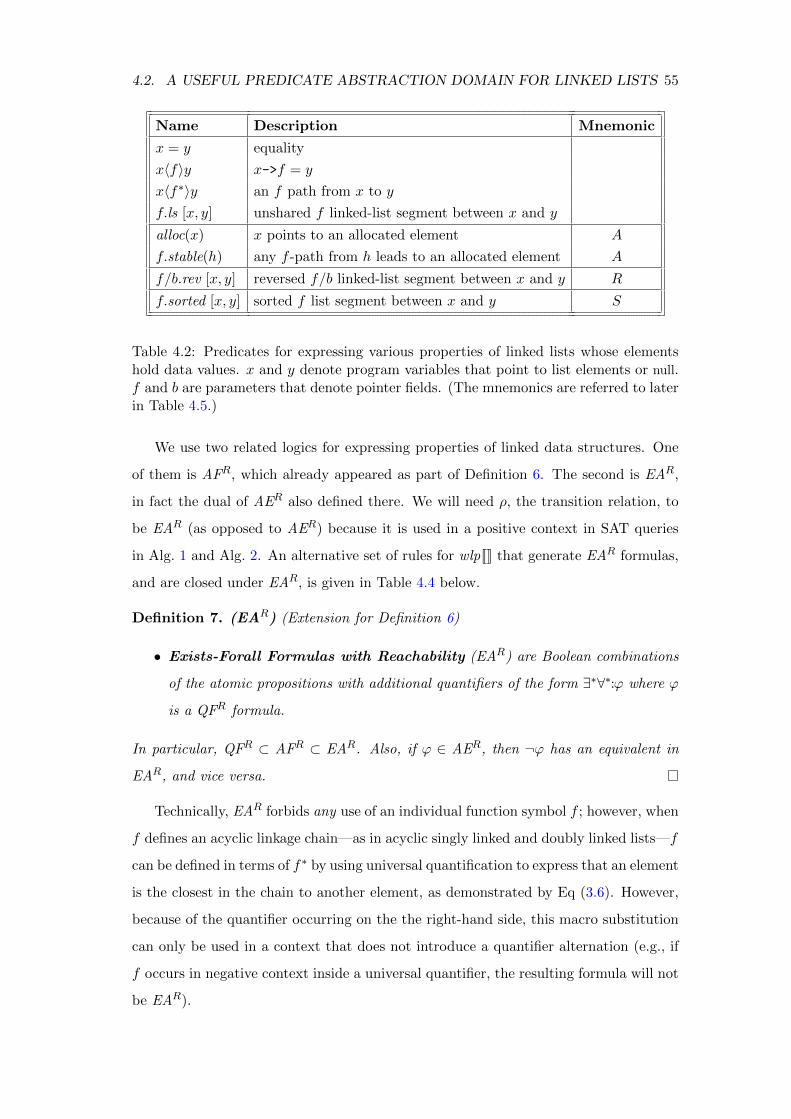
4.2. A USEFUL PREDICATE ABSTRACTION DOMAIN FOR LINKED LISTS 55
Name Description Mnemonic
x = y equality
x〈f〉y x->f = y
x〈f∗〉y an f path from x to y
f.ls [x, y] unshared f linked-list segment between x and y
alloc(x) x points to an allocated element A
f.stable(h) any f -path from h leads to an allocated element A
f/b.rev [x, y] reversed f/b linked-list segment between x and y R
f.sorted [x, y] sorted f list segment between x and y S
Table 4.2: Predicates for expressing various properties of linked lists whose elementshold data values. x and y denote program variables that point to list elements or null.f and b are parameters that denote pointer fields. (The mnemonics are referred to laterin Table 4.5.)
We use two related logics for expressing properties of linked data structures. One
of them is AFR, which already appeared as part of Definition 6. The second is EAR,
in fact the dual of AER also defined there. We will need ρ, the transition relation, to
be EAR (as opposed to AER) because it is used in a positive context in SAT queries
in Alg. 1 and Alg. 2. An alternative set of rules for wlp[[]] that generate EAR formulas,
and are closed under EAR, is given in Table 4.4 below.
Definition 7. (EAR) (Extension for Definition 6)
• Exists-Forall Formulas with Reachability (EAR) are Boolean combinations
of the atomic propositions with additional quantifiers of the form ∃∗∀∗:ϕ where ϕ
is a QFR formula.
In particular, QFR ⊂ AFR ⊂ EAR. Also, if ϕ ∈ AER, then ¬ϕ has an equivalent in
EAR, and vice versa.
Technically, EAR forbids any use of an individual function symbol f ; however, when
f defines an acyclic linkage chain—as in acyclic singly linked and doubly linked lists—f
can be defined in terms of f∗ by using universal quantification to express that an element
is the closest in the chain to another element, as demonstrated by Eq (3.6). However,
because of the quantifier occurring on the the right-hand side, this macro substitution
can only be used in a context that does not introduce a quantifier alternation (e.g., if
f occurs in negative context inside a universal quantifier, the resulting formula will not
be EAR).

56 CHAPTER 4. LOOP INVARIANTS
Name Formula
x〈f〉y Ef (x, y)
f.ls [x, y] ∀α, β : x〈f∗〉α ∧ α〈f∗〉y ∧ β〈f∗〉α =⇒ (β〈f∗〉x ∨ x〈f∗〉β)
f.stable(h) ∀α : h〈f∗〉α =⇒ alloc(α)
f/b.rev [x, y] ∀α, β :
(α 6= null ∧ β 6= null
∧ x〈f∗〉α ∧ α〈f∗〉y ∧ x〈f∗〉β ∧ β〈f∗〉y
)→(α〈f∗〉β ↔ β〈b∗〉α
)f.sorted [x, y] ∀α, β :
(α 6= null ∧ β 6= null
∧ x〈f∗〉α ∧ α〈f∗〉β ∧ β〈f∗〉y
)→ dle(α, β)
Table 4.3: AFR formulas for the derived predicates shown in Table 4.2. f and b denotepointer fields. dle is an uninterpreted predicate that denotes a total order on the datavalues. The intention is that dle(α, β) holds whenever α->d ≤ β->d, where d is the datafield. We assume that the semantics of dle are enforced by an appropriate total-orderbackground theory.
A Predicate Abstraction Domain that uses AFR
The abstraction predicates used for verifying properties of linked list programs were
introduced informally in Table 4.2. Table 4.3 gives the corresponding formal definition
of the predicates as AFR formulas. Note that all four predicates defined in Table 4.3
are quantified. (The quantified formula for Ef is given in Eq (3.6).) In essence, we use
a template-based approach for obtaining quantified invariants: the discovered invari-
ants have a quantifier-free structure, but the atomic formulas can be quantified AFR
formulas. Restricting the formulas in such a manner makes sure that the resulting
satisfiability checks in Alg. 2 would be of EAR formulas.
We now show that the EAR logic satisfies requirements R1 and R2 for the PDR
algorithm stated in Section 4.1.
Decidability of EAR
To satisfy requirement R1 stated in Section 4.1, we have to show that EAR is decidable
for satisfiability.
EAR is decidable for satisfiability because any formula in this logic can be translated
into the “effectively propositional” decidable logic of ∃∗∀∗ formulas described by Piskac
et al. [51]. EAR includes relations of the form f∗ (the reflexive transitive closure of a
function symbol f), but only allows limited use of f itself.
Every EAR formula can be translated into an ∃∗∀∗ formula using the the same
steps as in Section 3.2: (i) add a new uninterpreted relation Rf , which is intended to

4.2. A USEFUL PREDICATE ABSTRACTION DOMAIN FOR LINKED LISTS 57
Command C wlp[[C]](Q)
assume ϕ ϕ→ Q
x = y Q[y/x]
x = y->f y 6= null ∧ ∃α : (y〈f〉α ∧Q[α/x])
x->f = null x 6= null ∧Q[α〈f∗〉β ∧ (¬α〈f∗〉x ∨ β〈f∗〉x)/α〈f∗〉β]
x->f = y x 6= null ∧Q[α〈f∗〉β ∨ (α〈f∗〉x ∧ y〈f∗〉β)/α〈f∗〉β]
x = malloc() ∃α : ¬alloc(α) ∧Q[(alloc(β) ∨ (β = α ∧ β = x))/alloc(β))]
free(x) alloc(x) ∧Q[(alloc(β) ∧ β 6= x)/alloc(β))]
Table 4.4: A revised set of basic wlp[[]] rules for invariant inference. y〈f〉α is theuniversal formula defined in Eq (3.6). alloc stands for a memory location that has beenallocated and not subsequently freed.
represent reflexive transitive reachability via f ; (ii) add the consistency rule ΓlinOrd
shown in Table 3.2, which asserts that Rf is a partial order, i.e., reflexive, transitive,
acyclic, and linear;3 and (iii) replace all occurrences of t1〈f∗〉t2 by Rf (t1, t2). (By means
of this translation step, acyclicity is built into the logic.)
Proposition 4 (Simulation of EAR). Consider EAR formula ϕ over vocabulary
V = 〈C,F ,R〉. Let ϕ′ def= ϕ[Rf (t1, t2)/t1〈f∗〉t2]. Then ϕ′ is a first-order formula over
vocabulary V ′ = 〈C, ∅,R∪ {Rf : f ∈ F〉, and ΓlinOrd∧ϕ′ is satisfiable if and only if the
original formula ϕ is satisfiable.
This proposition is the dual of Proposition 2 for validity of ∀∗∃∗ formulas.
Axiomatic specification of concrete semantics in EAR
To satisfy requirement R2 stated in Section 4.1, we have to show that the transition
relation for each statement Cmd of the programming language can be expressed as a
two-vocabulary formula ρ ∈ EAR, where each program state variable is represented
by two constants: c, representing the value of the variable in the pre-state, and c′
representing the value of the variable in the post-state. Similarly, each pointer field is
represented by two binary relations f∗ and f ′∗ denoting reachability along f -paths in
pre- and post-states, respectively.
Let wlp[[Cmd]](Q) be the weakest liberal precondition of command Cmd with respect
to Q ∈ EAR. Then, the transition formula for command Cmd is wlp[[Cmd]](Id), where
3Note that the order is a partial order and not a total order, because not every pair of elementsmust be ordered.

58 CHAPTER 4. LOOP INVARIANTS
Id is a two-vocabulary formula that specifies that the input and the output states are
identical, i.e.,
Iddef=∧c∈C
c = c′ ∧∧f∈F∀α, β : α〈f∗〉β ⇔ α〈f ′∗〉β.
To show that the concrete semantics of linked list programs can be expressed in
EAR, we have to prove that EAR is closed under wlp[[ ]]; that is, for all commands Cmd
and Q ∈ EAR, wlp[[Cmd]](Q) ∈ EAR.
Table 4.4 shows rules for computing wlp of atomic commands. This is slightly re-
vised from Table 3.3 which generates ∃∗∀∗ formulas instead of ∀∗∃∗. Note that pointer-
related rules in Table 4.4 each include a memory-safety condition to detect null-
dereferences. For instance, the rule for “x->f = y” includes the conjunct “x 6= null”;
if, in addition, we wish to detect accesses to unallocated memory, the rule would be
extended with the conjunct “alloc(x)”.
The following lemma establishes the soundness and completeness of the wlp rules.
Lemma 1. Consider a command C of the form defined in Table 4.4 and postcondition
Q. Then, σ |= wlp[[C]](Q) if and only if the execution of C on σ can yield a state σ′
such that σ′ |= Q.
This lemma is the dual of Theorem 5 (Appendix A.2) for validity of ∀∗∃∗ formulas.
Consider a program with a single loop “while Cond do Cmd”. Alg. 1 can be
used to prove whether or not a precondition Pre ∈ AFR before the loop implies that a
postcondition Post ∈ AFR holds after the loop, if the loop terminates: we supply Alg. 1
with Initdef= Pre, ρ
def= Cond ∧ wlp[[Cmd]](Id) and Bad
def= ¬Cond ∧ ¬Post. Furthermore,
memory safety can be enforced on the loop body by setting Baddef= (¬Cond∧¬Post)∨
(Cond ∧ ¬wlp[[Cmd]](true).
4.3 Empirical Results
Summary
• The PDR framework was implemented, parametric of the abstraction predicates • Instantiated
with different subsets of predicates • Z3 was again used for generating models and unsat-cores •
Tested on a set of programs with linked lists • Invariants were successfully generated for correct
programs • We were also able to detect concrete bugs when introduced •

4.3. EMPIRICAL RESULTS 59
Benchmark
Memory-safety
+ data-structure integrity Additional properties
A Time N # calls to Z3 # clauses A Time N # calls to Z3 # clauses
create 1.37 3 28 3 8.19 4 96 7
delete 14.55 4 61 6 9.32 3 67 7
deleteAll A 6.77 3 72 6 A 37.35 7 308 12
filter 2.37 3 27 4 55.53 5 94 5
insert 26.38 5 220 16 25.25 4 155 13
prev 0.21 2 3 0 11.64 4 118 6
last 0.33 2 3 0 7.49 3 41 4
reverse 5.35 5 128 4 146.42 6 723 11
sorted insert S 41.07 3 48 7 S 51.46 4 134 10
sorted merge 26.69 4 87 10 S 256.41 5 140 14
make doubly-linked 18.91 3 44 5 R 1086.61 5 112 8
Table 4.5: Experimental results. Column A signifies the set of predicates used (blank= only the top part of Table 4.2; S = with the addition of the sorted predicate family;R = with the addition of the rev family; A = with the addition of the stable family,where alloc conjuncts are added in wlp rules). Running time is measured in seconds.N denotes the highest index for a generated element R[i]. The number of clauses refersto the inferred loop invariant.
To evaluate the usefulness of the analysis algorithm, we applied it to a collection
of sequential procedures that manipulate singly and doubly-linked lists (see Table 4.5).
For each program, we report the predicates used, the time (in seconds), the number of
PDR frames, the number of calls to Z3, and the size of the resulting inductive invariant,
in terms of the number of clauses. All experiments were run on a 1.7GHz Intel Core
i5 machine with 4GB of RAM, running OS X 10.7.5. We used version 4.3.2 of Z3 [11],
compiled for a 64-bit Intel architecture (using gcc 4.2 and LLVM).
For each of the benchmarks, we verified that the program avoids null-dereferences,
as well as that it preserves the data-structure invariant that the inputs and outputs
are acyclic linked-lists. In addition, for some of the benchmarks we were also able to
verify some additional correctness properties. While full functional correctness, or even
partial correctness, is hard to achieve using predicate abstraction, we were able to use
simple formulas to verify several interesting properties that go beyond memory-safety
properties and data-structure invariants. Table 4.6 describes the properties we checked
for the various examples. As seen from columns 3, 4, 8, and 9 of the entries for delete
and insert in Table 4.5, trying to prove stronger properties can sometimes result in fewer
iterations being needed, resulting in a shorter running time. In the remainder of the
examples, handling additional properties beyond memory-safety properties and data-

60 CHAPTER 4. LOOP INVARIANTS
Benchmark Property checked
create Some memory location pointed to by x (a global variable) thatwas allocated prior to the call, is not reachable from the list head,h.
delete The argument x is no longer reachable from h.
deleteAll An arbitrary non-null element x of the list becomes non-allocated.
filter Two arbitrary elements x and y that satisfy the filtering criterionand have an n-path between them, maintain that path.
insert The new element e is reachable from h and is the direct predecessorof the argument x.
last The function returns the last element of the list.
prev The function returns the element just before x, if one exists.
reverse If x comes before y in the input, then x should come after y in theoutput.
sorted insert The list rooted at h remains sorted.
make doubly-linked The resulting p is the inverse of n within the list rooted at h.
Table 4.6: Some correctness properties that can be verified by the analysis procedure.For each of the programs, we have defined suitable Pre and Post formulas in AFR.
Automatic bug finding
Benchmark Bug description Time N # calls to Z3 c.e. size
insert Precondition is too weak (omitted e 6=null)
4.46 1 17 8
filter Potential null dereference 6.30 1 21 3
Typo: list head used instead of list it-erator
103.10 3 79 4
reverse Corrupted data structure: a cycle iscreated
0.96 1 9 2
Table 4.7: Results of experiments with buggy programs. Running time is measured inseconds. N denotes the highest index for a generated element R[i]. “C.e. size” denotesthe largest number of individuals in a model in the counterexample trace.
structure invariants required more processing effort, which can be attributed mainly to
the larger set of symbols (and hence predicates) in the computation.
Bug Finding
We also ran our analysis on programs containing deliberate bugs, to demonstrate the
utility of this approach to bug finding. In all of the cases, the method was able to detect
the bug and generate a concrete trace in which the safety or correctness properties are
violated. The output in that case is a series of concrete states σ0..σN where each σi
contains the set of heap locations, pointer references, and program variables at step i.
The experiments and their results are shown in Table 4.7. We found both the length of

4.3. EMPIRICAL RESULTS 61
the trace and the size of the heap structures to be very small. Their small size makes
the traces useful to present to a human programmer, which can help in locating and
fixing the bug.
Observations
It is worth noting that for programs where the proof of safety is trivial—because every
access is guarded by an appropriate conditional check, such as in prev and last—
the algorithm terminates almost immediately with the correct invariant true. This
behavior is due to the property-directedness of the approach, in contrast with abstract
interpretation, which always tries to find the least fixed point, regardless of the desired
property.
We experimented with different refinements of inductive-generalization (Sec-
tion 4.1). Our algorithm could in many cases succeed even without minimizing the
unsat-core, but we observed runs with up to N = 40 iterations. On the other hand, the
more advanced versions of inductive generalization did not help us: trying to remove
literals resulted in a large number of expensive (and useless) solver calls; and blocking
spurious counter-examples using inductive generalization also turned out to be quite
expensive in our setting.
We also noticed that the analysis procedure is sensitive to the number of abstraction
predicates used. In particular, using predicates whose definitions involve quantifiers
can affect the running time considerably. When the predicate families f.sorted [x, y]
and f/b.rev [x, y] are added to A, running times can increase substantially (about 20-
60 times), as the space of formulas grows much larger. This effect occurred even in
the case of sorted merge, where we did not attempt to prove an additional correctness
property beyond safety and integrity—and indeed there were no occurrences of the
added predicates in the loop invariant obtained. As can be seen from Table 4.5, the
PDR algorithm per se is well-behaved, in the sense that the number of calls to Z3
increased only modestly with the additional predicates. However, each call to Z3 took
a lot more time.
In make doubly-linked, proving the prev/next-inverse property requires the predicate
family f/b.rev [x, y] (see Table 4.3), resulting in a slowdown of more than twenty times
over just proving safety and integrity (without the use of the f/b.rev [x, y] predicates).
For sorted merge, we did not prove an additional correctness property beyond safety and

62 CHAPTER 4. LOOP INVARIANTS
integrity; the numbers reported in columns 6–9 are for proving safety and integrity when
the predicate family f.sorted [x, y] is also included. These predicates are not needed
to prove safety and integrity, nor did they show up in the resulting invariant; however,
the analysis time was more than sixty times slower than was needed to prove safety
and integrity without the additional predicates, and two orders of magnitude slower
than delete and insert. As can be seen from column 4, about the same number of
calls to Z3 were performed for all four examples; however, in the case of (the extended)
sorted merge and make doubly-linked, each call to Z3 took a lot more time.
4.4 Related Work for Chapter 4
The literature on program analysis is vast, and the subject of shape analysis alone has
an extensive literature. Thus, in this section we are only able to touch on a few pieces
of prior work that relate to the ideas used in this chapter.
Predicate abstraction. Houdini [16] is the first algorithm of which we are aware
that aims to identify a loop invariant, given a set of predicates as candidate ingredients.
However, Houdini only infers conjunctive invariants from a given set of predicates.
Santini [64, 65] is a recent algorithm for discovering invariants expressed in terms of
a set of candidate predicates. Like our algorithm, Santini is based on full predicate
abstraction (i.e., it uses arbitrary Boolean combinations of a set of predicates), and
thus is strictly more powerful than Houdini. Santini could make use of the predicates
and abstract domain described in this chapter; however, unlike our algorithm, Santini
would not be able to report counterexamples when verification fails. Other work infers
quantified invariants [31, 61] but does not support the reporting of counterexamples.
Templates are used in many tools to define the abstract domains used to represent sets
of states, by fixing the form of the constraints permitted. Template Constraint Matrices
[60] are based on inequalities in linear real arithmetic (i.e., polyhedra), but leave the
linear coefficients as symbolic inputs to the analysis. The values of the coefficients are
derived in the course of running the analysis. In comparison, a coefficient in our use
of EAR corresponds to one of the finitely many constants that appear in the program,
and we instantiated our templates prior to using PDR.
As mentioned in the beginning of this chapter, PDR meshes well with full pred-
icate abstraction: in effect, the analysis obtains the benefit of the precision of the

4.4. RELATED WORK FOR CHAPTER 4 63
abstract transformers for full predicate abstraction, without ever constructing the ab-
stract transformers explicitly. PDR also allows a predicate-abstraction-based tool to
create concrete counterexamples when verification fails.
Abstractions based on linked-list segments. Our abstract domain is based on
formulas expressed in AFR, which has very limited capabilities to express properties
of stretches of data structures that are not pointed to by a program variable. This
feature is similar to the self-imposed limitations on expressibility used in a number
of past approaches, including (a) canonical abstraction [59]; (b) a prior method for
applying predicate abstraction to linked lists [47]; (c) an abstraction method based on
“must-paths” between nodes that are either pointed to by variables or are list-merge
points [43]; and (d) domains based on separation logic’s list-segment primitive [6, 14]
(i.e., “ls[x, y]” asserts the existence of a possibly empty list segment running from the
node pointed to by x to the node pointed to by y). Decision procedures have been
used in previous work to compute the best transformer for individual statements that
manipulate linked lists [52, 68].
STRAND and elastic quantified data automata. Recently, Garg et al. devel-
oped methods for obtaining quantified invariants for programs that manipulate linked
lists via an abstract domain of quantified data automata [21, 22]. To create an abstract
domain with the right properties, they use a weakened form of automaton—so-called
elastic quantified data automata—that is unable to observe the details of stretches
of data structures that are not pointed to by a program variable. (Thus, an elastic
automaton has some of the characteristics of the work based on linked-list segments
described above.) An elastic automaton can be converted to a formula in the decidable
fragment of the STRAND logic over lists [45].
Other work on IC3/PDR. Our work represents the first application of PDR to
programs that manipulate dynamically allocated storage. We chose to use PDR because
it has been shown to work extremely well in other domains, such as hardware verification
[8, 15]. Subsequently, it was generalized to software model checking for program models
that use linear real arithmetic [30] and linear rational arithmetic [9]. Cimatti and
Griggio [9] employ a quantifier-elimination procedure for linear rational arithmetic,
based on an approximate pre-image operation. Our use of a predicate-abstraction

64 CHAPTER 4. LOOP INVARIANTS
domain allows us to obtain an approximate pre-image as the unsat core of a single call
to an SMT solver (line 2 of Alg. 2).

Chapter 5
Modular Analysis of Procedures
This chapter is based on the results published in [37].
This chapter shows how to harness existing SAT solvers for proving that a program
containing (potentially recursive) procedures satisfies its specification and for auto-
matically producing counterexamples when it does not. We concentrate on proving
safety properties of imperative programs manipulating linked data structures which is
challenging since we need to reason about unbounded memory and destructive pointer
updates. The tricky part is to identify a logic which is expressive enough to enable
the modular verification of interesting procedures and properties and weak enough to
enable sound and complete verification using SAT solvers.
In the previous chapters we have shown how to employ effectively propositional
logic for verifying programs manipulating linked lists. However, we see that effectively
propositional logic does not suffice to naturally express the effect on the global heap
when the local heap of a procedure is accessible via shared nodes from outside. For
example, Fig. 5.1 shows a pre- and post-heap before a list pointed-to by h is reversed.
The problem is how to express the change in reachability between nodes such as zi
1h 2 3 4 5
z1 z2 z3
;reverse x
1 2 3 4 5 h
z1 z2 z3
Figure 5.1: Reversing a list pointed to by a head h with many shared nodes accessiblefrom outside the local heap (surrounded by a rounded rectangle).
65
66 CHAPTER 5. MODULAR ANALYSIS OF PROCEDURES
and list nodes 1, 2, . . . , 5: note that, e.g., nodes 3, 4, 5 are unreachable from z1 in the
post-heap.
This chapter shows that in many cases, including the above example, reachability
can still be checked precisely using SAT solvers. Our solution is based on the following
principles:
• We follow the standard techniques (e.g., see [4, 41, 66, 71]) by requiring that the
programmer define the set of potentially modified elements.
• The programmer only specifies postconditions on local heaps and ignores the
effect of paths from the global heap.
• We provide a general and exact adaptation rule for adapting postconditions to
the global heap. This adaptation rule is expressible in a generalized version of
AER (Definition 6) called AEAR. AEAR allows an extra function symbol, called
the entry function, that maps each node u in the global heap into the first node
accessible from u in the local heap. In Fig. 5.1, z1, z2 and z3 are mapped to
2, 3 and 4, respectively. The key facts are that AEAR suffices to precisely define
the global reachability relationship after each procedure call and yet any AEAR
formula can be simulated by an AER formula, and from Proposition 2, by an
effectively propositional one. Thus the automatic methods used in Chapter 3 still
apply to this significantly more general setting.
• We restrict the verified procedures in order to guarantee that the generated ver-
ification condition of every procedure remains in AEAR. The main restrictions
are: type correctness, deterministic paths in the heap, limited number of changed
list segments in the local heap (each of which may be unbounded) and limited
amount of newly created heap sharing by each procedure call. These restrictions
are enforced by the generated verification condition in AEAR. This formula is
automatically checked by the SAT solver.
Main Results
The results presented in this chapter can be summarized as follows:
• We define a new logic, AEAR, which extends the previously defined AER (Defini-
tion 6) with a limited idempotent function and yet is equi-satisfiable with EPR.

5.1. THE PROBLEM WITH GLOBAL STATE 67
• We provide a precise adaptation rule in AEAR, expressing the locality property
of the change, such that, in conjunction with the formula expressing the post-
condition of the local heap, it precisely updates the reachability relation over the
global heap.
• We generate a modular verification formula in AEAR for each procedure, asserting
that the procedure satisfies its pre- and post-conditions and the above restrictions.
This verification condition is sound and complete, i.e., it is valid if and only if the
procedure adheres to the restrictions and satisfies its requirements.
• We implemented this tool on top of Z3. We were able to show that many programs
can be modularly verified using our methods. They satisfy our restrictions and
their invariants can be expressed naturally in AER.
5.1 The Problem with Global State
5.1.1 A Running Example
To make the discussion more clear, we start with an example program. We use the
union-find data structure, due to Tarjan [62], which efficiently maintains a partition of
elements, supporting the union of two bins and giving each bin a unique representative.
It does so by maintaining a forest using a parent pointer at each node (see Fig. 5.2). 1,
Two elements are in the same bin iff they share a common root.
The method find requires that the argument x is not null. The formula tailf (x, rx)
means that the last node on an f -path from x is rx, which asserts that the auxiliary
variable rx is equal to the root of x. The procedure changes the pointers of some nodes
in the list segment between x and rx, denoted using the closed interval [x, rx]f . All the
nodes in this segment are set to point directly to rx.
The return value of find (denoted by retval) is rx. The postcondition uses the
symbol f denoting the value of f before the method was invoked. Since find compresses
paths from ancestors of x to single edges to rx, this root may be shared via new parent
pointers. Fig. 5.3 depicts a typical run of find.
The method union requires that both its arguments are not null. It potentially
modifies the ancestors of x and y, i.e., [x, rx]f ∪ [y, ry]f . Fig. 5.4 depicts a typical run
1We have simplified union by not keeping track of the sizes of sets (usually employed in order toattach the smaller set to the larger).
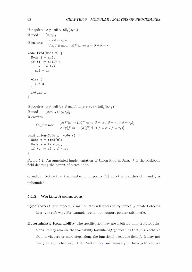
68 CHAPTER 5. MODULAR ANALYSIS OF PROCEDURES
@ requires x 6= null ∧ tailf (x, rx)
@ mod [x, rx]f
@ ensuresretval = rx ∧∀α, β ∈ mod : α〈f∗〉β ↔ α = β ∨ β = rx
Node find(Node x) {Node i = x.f;
if (i != null) {i = find(i);
x.f = i;
}else {i = x;
}return i;
}
@ requires x 6= null ∧ y 6= null ∧ tailf (x, rx) ∧ tailf (y, ry)
@ mod [x, rx]f ∪ [y, ry]f
@ ensures
∀α, β ∈ mod :
(x〈f∗〉α→ (α〈f∗〉β ↔ β = α ∨ β = rx ∨ β = ry)
)∧(y〈f∗〉α→ (α〈f∗〉β ↔ β = α ∨ β = ry)
)void union(Node x, Node y) {
Node t = find(x);
Node s = find(y);
if (t != s) t.f = s;
}
Figure 5.2: An annotated implementation of Union-Find in Java. f is the backbonefield denoting the parent of a tree node.
of union. Notice that the number of cutpoints [56] into the branches of x and y is
unbounded.
5.1.2 Working Assumptions
Type correct The procedure manipulates references to dynamically created objects
in a type-safe way. For example, we do not support pointer arithmetic.
Deterministic Reachability The specification may use arbitrary uninterpreted rela-
tions. It may also use the reachability formula α〈f∗〉β meaning that β is reachable
from α via zero or more steps along the functional backbone field f . It may not
use f in any other way. Until Section 6.2, we require f to be acyclic and we
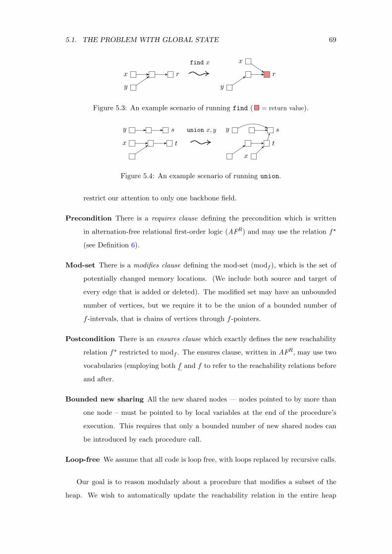
5.1. THE PROBLEM WITH GLOBAL STATE 69
x r
y
;find x x
r
y
Figure 5.3: An example scenario of running find ( = return value).
x t
y s
;union x, y
x
t
y s
Figure 5.4: An example scenario of running union.
restrict our attention to only one backbone field.
Precondition There is a requires clause defining the precondition which is written
in alternation-free relational first-order logic (AFR) and may use the relation f?
(see Definition 6).
Mod-set There is a modifies clause defining the mod-set (modf ), which is the set of
potentially changed memory locations. (We include both source and target of
every edge that is added or deleted). The modified set may have an unbounded
number of vertices, but we require it to be the union of a bounded number of
f -intervals, that is chains of vertices through f -pointers.
Postcondition There is an ensures clause which exactly defines the new reachability
relation f? restricted to modf . The ensures clause, written in AFR, may use two
vocabularies (employing both f and f to refer to the reachability relations before
and after.
Bounded new sharing All the new shared nodes — nodes pointed to by more than
one node – must be pointed to by local variables at the end of the procedure’s
execution. This requires that only a bounded number of new shared nodes can
be introduced by each procedure call.
Loop-free We assume that all code is loop free, with loops replaced by recursive calls.
Our goal is to reason modularly about a procedure that modifies a subset of the
heap. We wish to automatically update the reachability relation in the entire heap

70 CHAPTER 5. MODULAR ANALYSIS OF PROCEDURES
x
c
yz
modf
modf∗
;find x
x
c
yz
modf
modf∗
Figure 5.5: A case where changes made by find have a non-local effect: y〈f∗〉c, but¬y〈f∗〉c.
based on the changes to the modified subset. We remark that we are concerned with
reachability between any two nodes in the heap, as opposed to only those pointed to
by program variables. When we discuss sharing we mean sharing via pointer fields in
the heap as opposed to aliasing from stack variables, which does not concern us in this
context.
5.1.3 Non-Local Effects
Reachability is inherently non-local: a single edge mutation can affect the reachability
of an unbounded number of points that are an unbounded distance from the point of
change. Fig. 5.5 contains a typical run of find. Two kinds of “frames” are depicted:
(i) modf = [x, rx)f , specified by the programmer, denotes the nodes whose edges can be
directly changed by find— this is the standard notion of a frame condition; (ii) modf∗
denotes nodes for which f∗, the reachability relation, has changed. We do not and
in general we cannot specify this set in a modular way because it usually depends
on variables outside the scope of the current function such as y in Fig. 5.5. In the
example shown, there is a path from y to c before the call which does not exist after
the call. Furthermore, modf∗ can be an arbitrarily large set: in particular, it may not
be expressible as the union of a bounded set of intervals: for example, when adding a
subtree as a child of some node in another tree, modf spans only one edge, whereas
modf∗ is the entire subtree added — which may contain an unbounded number of
branches.
The postcondition of find is sound (every execution of find satisfies it), but in-
complete: it does not provide a way to determine information concerning paths outside
mod, such as from y to c in Fig. 5.5. Therefore, this rule is often not enough to verify
the correctness of programs that invoke find in larger contexts.
Notice the difficulty of updating the global heap, especially the part modf∗ \modf .

5.2. AN ADAPTATION RULE FOR DETERMINISTIC TRANSITIVE CLOSURE71
mod
q f f
q q
q
f
f
f f
q
q q
Figure 5.6:Labeling edges inside and outside mod.
In particular, using only the local specification of find, one would not be able to prove
that ¬y〈f∗〉c. Indeed, the problem is updating the reachability of elements that are
outside mod; in more complex situations, these elements may be far from the changed
interval, and their number may be unbounded.
One possibility to avoid the problem of incompleteness is to specify a postcondition
which is specific to the context in which the invocation occurs. However, such a solution
requires reasoning per call site and is thus not modular. We wish to develop a rule that
will fit in all contexts. Reasoning about all contexts is naturally done by quantification.
5.2 An Adaptation Rule for Deterministic Transitive Clo-
sure
5.2.1 An FO(TC) Adaptation Rule
A standard way to modularize specifications is to specify the local effect of a procedure
and then to use a general adaptation rule (or frame rule) to derive the global effect. In
our case, we know that locations outside mod are not modified. Therefore, for example,
after a call to find a new path from node σ to node τ is either an old path from σ
to τ , or it consists of an old path to a node α ∈ mod, a new path from α to a node
β ∈ mod and an old path from β to τ :
∀σ, τ : σ〈f∗〉τ ↔ σ〈q∗〉τ ∨
∃α, β ∈ mod : σ〈q∗〉α ∧ α〈f∗〉β ∧ β〈q∗〉τ(5.1)

72 CHAPTER 5. MODULAR ANALYSIS OF PROCEDURES
α 1 2 3 4 α 1 2 3 4
α 1 2 3 4 α 1 2 3 4
(a) (b)
(c) (d)
del 〈2, 3〉 del 〈2, 3〉
Figure 5.7: Memory states with non-unique pointers where global reasoning aboutreachability is hard. In the memory state (a), there is one edge from α into the modified-set {1, 2, 3, 4}, and in memory state (b), there are two edges from α into the samemodified-set, {1, 2, 3, 4}. The two memory states have the same reachability relationand therefore are indistinguishable via reachability alone. The memory states (c) and(d) are obtained from the memory states (a) and (b), respectively, by deleting the edge〈2, 3〉. The reachability in (c) is not the same as in (d), which shows it is impossible toupdate reachability in general w.r.t. edge deletion, without using the edge relation.
Notice that the condition α ∈ mod is expressible as a quantifier-free formula using f∗
when mod is specified, as it is, as a union of intervals. Here q∗ denotes paths through
edges, that are definitely unchanged, since at least one of their ends is outside mod
(recall that f denotes f before the change) —
∀α, β : α〈q〉β ↔ α〈f〉β ∧ (α /∈ mod ∨ β /∈ mod) (5.2)
Thus we distinguish between edges that have both ends in mod, and therefore may
have been altered in a manner described by the “ensures” clause, and other edges,
which were not changed at all. We therefore define q (and hence, its transitive closure,
q∗) to be exactly all the edges “outside” mod, that is, having at least one end that
does not belong to mod (Eq (5.2)). Now we define all the new paths f∗ using q∗ and a
restriction of f∗ to only edges inside mod. See Fig. 5.6 for a depiction of these labels.
Every such new path is either constructed entirely of “old” edges q, or is constructed
from some path f∗ between two nodes α, β ∈ mod, concatenated with some old prefix
and some old suffix (each of which may be zero-length). This is expressed by Eq (5.1).
Taking the adaptation rule given by Eq (5.1) and Eq (5.2) eliminates superfluous
behaviours involving edges outside mod being changed. Notice that these equations
are not specific to find, but Eq (5.1) does assume that no new path can enter and exit
mod multiple times. In this formula α is a placeholder for an entry-point into mod and

5.2. AN ADAPTATION RULE FOR DETERMINISTIC TRANSITIVE CLOSURE73
β is a placeholder for an exit-point from mod.
The adaptation rule uses a logic which is too expressive and thus hard for automated
reasoning: FOTC is not decidable (in fact, not even recursively enumerable). The
first problem is that the q∗ relation is not usually first order expressible and generally
requires transitive closure. For example, Fig. 5.7 shows that in general the adaptation
rule is not necessarily definable using only the reachability relation, when there are
multiple outgoing edges per node. We avoid this problem by only reasoning about
functional fields, f .
The second problem with Eq (5.1) is that it contains quantifier alternation. α
matches an arbitrary node in mod which may be of arbitrary size. Therefore, it is not
completely obvious how to avoid existential quantifications.
5.2.2 An Adaptation Rule in a Restricted Logic
We provide an equivalent adaptation rule in a restricted logic, without extra quantifier-
alternations. Indeed, our assumptions from Section 5.1.2, especially the deterministic
reachability, single backbone field, acyclicity, and the bound on the number of intervals
in the mod-set, greatly simplify reasoning about modified paths in the entire heap. The
simplification is obtained by employing an additional unary function symbol enmod,
where enmod(σ) is meant to denote the entry point of the node σ in mod, that is the
first node on the (unique) path from σ that enters mod, and null if no such node exists
(see Fig. 5.8). Note that since transitive closure is only applied to functions, the entry
points such as α in Eq (5.1) is uniquely determined by σ, the origin of the path. A
key property of enmod is that on mod itself, enmod acts as identity, and therefore for
any σ ∈ V it holds that enmod(enmod(σ)) = enmod(σ)) — that is, the function enmod
is idempotent . It is important to note that enmod does not change as a result of local
modifications in mod. Hence, we do not need to worry about enmod in the pre-state as
opposed to the post-state, and we do not need to parametrize enmod by f/f . Formally,
enmod is characterized by the following formula:
∀σ : σ〈f∗〉enmod(σ) ∧ enmod(σ) ∈ mod ∧
∀α ∈ mod : σ〈f∗〉α→ enmod(σ)〈f∗〉α(5.3)
Using enmod the new adaptation rule adapt[mod] is obtained by considering, for

74 CHAPTER 5. MODULAR ANALYSIS OF PROCEDURES
. . .
mod
enmod
enmod
enmod : V → mod
Figure 5.8: The function enmod maps every node σ to the first node in mod reachablefrom σ. Notice that for any α ∈ mod, enmod(α) = α by definition.
σα t1
t2
mod
τ
. . .
Figure 5.9: This diagram depicts how an arbitrary path from σ /∈ mod to τ /∈ mod isconstructed from three segments: [σ, α]f , [α, ti]f , and [ti, τ ]f (here i = 2). Arrows inthe diagram denote paths; thick arrows entering and exiting the box denote paths thatwere not modified since they are outside of mod. Here, α = enmod(σ) is an entry-pointand t1, t2 are exit-points.
every source and target, the following three cases:
Out-In: The source is out of mod; the target is in;
In-Out: The source is in mod; the target is out;
Out-Out: The source and target are both out of mod.
The full adaptation rule is obtained by taking the conjunction of the formulas for
each case (Eq (5.4), Eq (5.5),Eq (5.6)), that are described below, and the formula
defining enmod (Eq (5.3)).
Out-In Paths Using enmod we can easily handle paths that enter mod. Such paths
originate at some σ /∈ mod and terminate at some τ ∈ mod. Any such path therefore
has to go through enmod(σ) as depicted in Fig. 5.9. Thus, the following simple formula
can be used:
∀σ /∈ mod, τ ∈ mod : σ〈f∗〉τ ↔ enmod(σ)〈f∗〉τ (5.4)
Observe that for some β ∈ mod, the atomic formula used above, enmod(σ)〈f∗〉β,
corresponds to the FO(TC) sub-formula ∃α : σ〈q∗〉α ∧ α〈f∗〉β from Eq (5.1).

5.2. AN ADAPTATION RULE FOR DETERMINISTIC TRANSITIVE CLOSURE75
@ requires Ef (x, f1x) ∧ Ef (f1x , f2x) ∧ Ef (f3x , f
2x)∧
x 6= null ∧ f1x 6= null ∧ f2x 6= null
@ mod [x, f3x ]
@ ensures . . .
void swap(Node x) {Node t = x.f;
x.f = t.f;
t.f = x.f.f;
x.f.f = t;
}
x
t
f3x
modn
Figure 5.10: A simple function that swaps two adjacent elements following x in asingly-linked list. Dotted lines denote the new state after the swap. The notation e.g.Ef (x, f1x) denotes the single edge from x to f1x following the f field.
In-Out Paths We now shift attention to paths that exit mod. Exit points, that is,
last points on some path that belong to mod, are more subtle since you need both
ends of the path to determine them. The end of the path is not enough since it can be
shared, and the origin of the path is not enough since it can exit the set multiple times,
because a path may exit mod and enter it again later. Therefore, we cannot define a
function in a similar manner to enmod. The fact that transitive closure is only applied
to functions is useful here: every interval [α, β] has at most one exit β. We therefore
utilize the fact that mod is expressed as a bounded union of intervals — which bounds
the potential exit points to a bounded set of terms. We will denote the exit points of
mod with ti.
For example, in the procedure swap shown in Fig. 5.10, mod = [x, f3x ] and there is
one exit point t1 = f3x (f3x is a constant set by the precondition to have the value of
f(f(f(x))) using the inversion formula Eq (3.6) introduced in Section 3.2.
Observe a general path that originates at some σ ∈ mod and terminates at some
τ /∈ mod (see Fig. 5.11). Evidently this path has to go though one of the ti s, which, as a
result of our assumptions, are bounded. Notice that the exit points, too, do not change
as a result of modifying edges between nodes in mod. Assume a path from σ to τ and
let ti be the last exit point along that path. This is important, because it lets us know
that the segment of the path between ti and τ comprises solely of unchanged edges —
since they are all outside of mod. We can therefore safely use f∗, rather than q∗, to
characterize it. As for the part of the path between σ and ti, it can be characterized
simply by f∗, because σ and ti are both in mod. Therefore the entire path can be
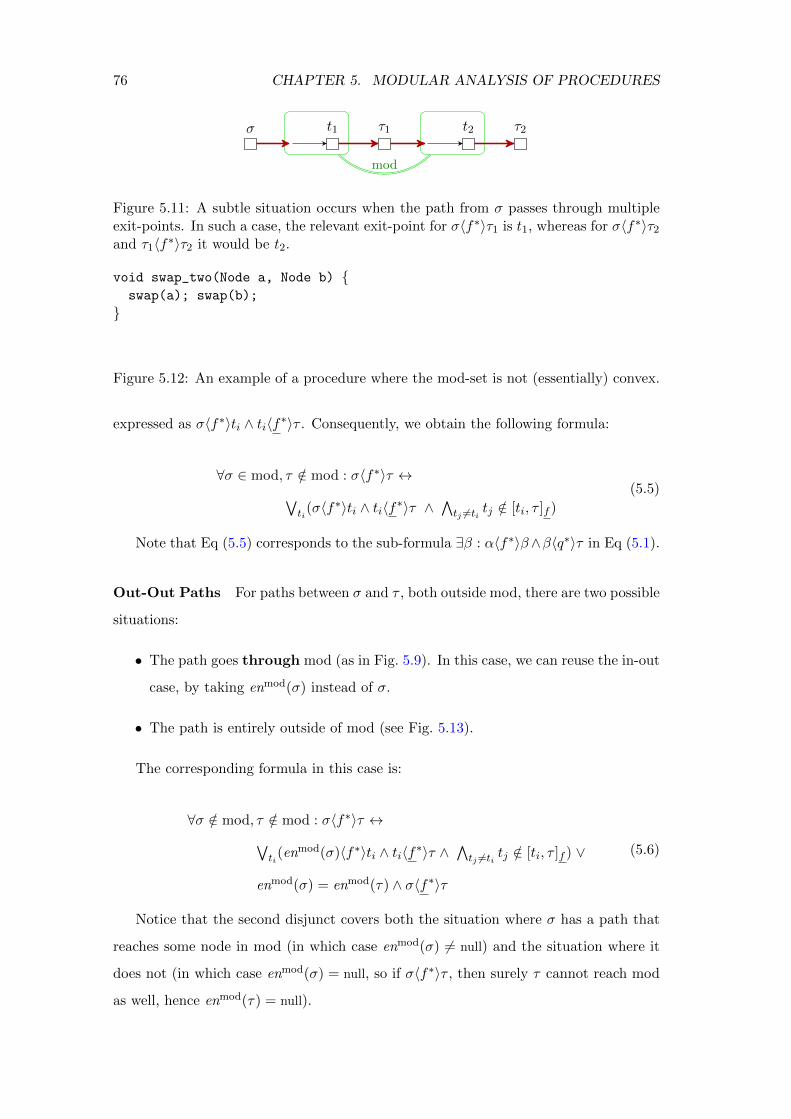
76 CHAPTER 5. MODULAR ANALYSIS OF PROCEDURES
σ t1 τ1 t2 τ2
mod
Figure 5.11: A subtle situation occurs when the path from σ passes through multipleexit-points. In such a case, the relevant exit-point for σ〈f∗〉τ1 is t1, whereas for σ〈f∗〉τ2and τ1〈f∗〉τ2 it would be t2.
void swap_two(Node a, Node b) {swap(a); swap(b);
}
Figure 5.12: An example of a procedure where the mod-set is not (essentially) convex.
expressed as σ〈f∗〉ti ∧ ti〈f∗〉τ . Consequently, we obtain the following formula:
∀σ ∈ mod, τ /∈ mod : σ〈f∗〉τ ↔∨ti
(σ〈f∗〉ti ∧ ti〈f∗〉τ ∧∧tj 6=ti tj /∈ [ti, τ ]f )
(5.5)
Note that Eq (5.5) corresponds to the sub-formula ∃β : α〈f∗〉β∧β〈q∗〉τ in Eq (5.1).
Out-Out Paths For paths between σ and τ , both outside mod, there are two possible
situations:
• The path goes through mod (as in Fig. 5.9). In this case, we can reuse the in-out
case, by taking enmod(σ) instead of σ.
• The path is entirely outside of mod (see Fig. 5.13).
The corresponding formula in this case is:
∀σ /∈ mod, τ /∈ mod : σ〈f∗〉τ ↔∨ti
(enmod(σ)〈f∗〉ti ∧ ti〈f∗〉τ ∧∧tj 6=ti tj /∈ [ti, τ ]f ) ∨
enmod(σ) = enmod(τ) ∧ σ〈f∗〉τ
(5.6)
Notice that the second disjunct covers both the situation where σ has a path that
reaches some node in mod (in which case enmod(σ) 6= null) and the situation where it
does not (in which case enmod(σ) = null, so if σ〈f∗〉τ , then surely τ cannot reach mod
as well, hence enmod(τ) = null).

5.2. AN ADAPTATION RULE FOR DETERMINISTIC TRANSITIVE CLOSURE77
σ1 τ1 α
σ2 τ2
mod
Figure 5.13: Paths that go entirely untouched. enmod(σ1) = α, whereas enmod(σ2) =null.
To conclude, given mod, adapt[mod] is the conjunction of the three formulas in
Eq (5.4), Eq (5.5), Eq (5.6), and the formula defining enmod (Eq (5.3)). To show its
adequacy, some more formalism is required, and it is introduced in the following section.
5.2.3 Adaptable Heap Reachability Logic
The utility of enmod in the formulas for adaptation motivates the definition of a logic
fragment that would be able to accommodate it.
Definition 8. The new logic AEAR is obtained by augmenting AER with unary function
symbols, denoted by g, h1, . . . , hn where:
• g should be interpreted as an idempotent function: g(g(α)
)= g(α).
• The images of h1, . . . , hn are all bounded by some pre-determined parameter N ,
that is: each hi takes at most N distinct values.
• All terms involving these function symbols have the form f(z), where z is some
variable.
We later show that AEAR suffices for expressing the verification conditions of the
programs discussed above. In the typical use case, the function g assigns the entry
point in the mod-set for every node (called enmodf above), and the functions h1, . . . , hn
are used for expressing the entry points in inner mod-sets. The main attractive feature
of this logic is given in the following theorem.
Theorem 4. Any AEAR-formula ϕ can be translated to an equal-valid (first-order)
function-free ∀∗∃∗-formula.
The proof of Theorem 4, given in Appendix A.4, begins by translating ϕ to a ∀∗∃∗-formula ϕ′ as described in Proposition 2, keeping the function symbols g, h1, . . . , hn as is.
These function symbols are then replaced by additional relation and constant symbols,

78 CHAPTER 5. MODULAR ANALYSIS OF PROCEDURES
and extra universal relational formulas are used to enforce the semantic restrictions of
them.
5.3 Extending wlp for Procedure Calls
5.3.1 Modular Specifications of Procedure Behaviours
Here we explain how procedure specifications are written in order to support modular
verification.
Definition 9. A vocabulary V = 〈C, {f},R〉 is a triple of constant symbols, a function
symbol, and relation symbols. The special constant symbol null is always included. A
state, M , is a logical structure with universe |M |, including null, and nullM = null =
fM (null).2 A state is appropriate for an annotated procedure proc if its vocabulary
includes every symbol occurring in its annotations, and constants corresponding to all
of the program variables occurring in proc.
The diagrams in this chapter denote program states. For example Fig. 5.1 shows a
transition between two states.
Definition 10 (Backbone Differences). For states M and M with the same domain
(|M| = |M | denotes the domain of M), we denote by M/M the structure over the two-
vocabulary V = 〈{null} ∪ C ∪ C, {f, f},R∪R〉 obtained by combining M and M in the
obvious way. The set M ⊕M consists of the “differences between M and M excluding
null”, i.e. M ⊕M = {u : fM (u) 6= fM (u)} ∪ {fM (u) : fM (u) 6= fM (u)} \ {null}.
Modification Set
We must specify the mod-set, mod, containing all the endpoints of edges that are
modified. Therefore when adding or deleting an edge 〈s, t〉, both ends — the source, s,
and the target, t — are included in mod. Often in programming language semantics,
only the source is considered modified. However, thinking of the heap as a graph, it is
useful to consider both ends of a modified edge as modified.
Our mod-sets are built from two kinds of intervals:
2Remember that nullM is the interpretation of null in the structure M , and fM is the interpretationof f .

5.3. EXTENDING WLP FOR PROCEDURE CALLS 79
Command Pre Mod Post
ret = y.f y 6= null ∧ Ef (y, s) ∅ ret = s
y.f = null y 6= null ∧ Ef (y, s) [y, s]f ¬y〈f∗〉s ∧ ¬s〈f∗〉yassume y.f==null;
y.f = x y 6= null ∧ Ef (y, null) ∧ ¬x〈f∗〉y [y, y]f ∪ [x, x]f y〈f∗〉x ∧ ¬x〈f∗〉y
Table 5.1: The specifications of atomic commands. s is a local constant denoting thef -field of y. Ef is the inversion formula defined in Eq (3.6).
Definition 11 (Intervals). The closed interval [a, b]f is
[a, b]fdef= {α | a〈f∗〉α ∧ α〈f∗〉b}
and the half-open interval [a, null)f is:
[a, null)fdef= {α | a〈f∗〉α ∧ α〈f+〉null}
(notice that α〈f+〉null is trivially true in acyclic heaps).
Definition 12 (mod-set). The mod-set, mod, of a procedure is a union I1∪I2∪ . . .∪Ik,
where each Ii may be [si, ti]f or [si, null)f , si, ti are parameters of the procedure or
constant symbols occurring in the pre-condition.
In our examples, the mod-sets of find and union are written above each procedure,
preceded by the symbol “@ mod” (Fig. 5.2). Note that it follows from Definition 12
that “α ∈ mod” is expressible as a quantifier-free formula.
Definition 13. Given an appropriate state M for proc with modset mod, modM is
the set of all elements in |M | that are in mod (where mod is defined by a union of
intervals, see Definition 11).
Pre- and Post-Conditions
The programmer specifies AFR pre- and post-conditions. Two-vocabulary formulas
may be used in the post-conditions where f denotes the value of f before the call.

80 CHAPTER 5. MODULAR ANALYSIS OF PROCEDURES
Specifying Atomic Commands
Table 5.1 provides specification of atomic commands. They describe the memory
changed by atomic statements and the changes on the local heap.
Accessing a pointer field The statement ret = y.f reads the content of the f -
field of y into ret. It requires that y is not null and that an auxiliary variable s point
to the f -field of y (which may be null). It does not modify the heap at all. It sets
ret to s. It is interesting to note that the postcondition is much simpler than the one
provided in Section 3.4 because there is no need to specify the effect on the whole heap.
In particular, it does not employ quantifiers at all. The quantification is “filled in” by
the adaptation rule.
Edge Removals The statement y.f = null sets the content of the f -field of y, into
null. It requires that y is not null and that an auxiliary variable s points to the f -field
of y (which may be null). It modifies the node pointed-to by y and potentially the
node pointed-to by s. Notice that the modset includes two elements pointed by y and
t, the two end-points of the edge. It removes paths between y and s. The postcondition
assert that there are no paths from y to s. Also, since s is potentially modified, it has
to assert that no path is created from s to y.
Edge Additions The statement y.f = x is specified assuming without loss of gener-
ality, that the statement y.f = null was applied before it. Thus, it only handles edge
additions. It therefore requires that y is not null and its f -field is null. It modifies the
node pointed-to by y and potentially the node pointed-to by x. It creates a new path
from y to x and asserts the absence of new paths from x back to y. Again the absence
of back paths (denoted by ¬x〈f∗〉y) is needed for completeness. The reason is that
both the node pointed-to by x and y are potentially modified. Since x is potentially
modified, without this assertion, a post-state in which x.f == y will be allowed by the
postcondition.
5.3.1.1 Soundness and Completeness
We now formalize the notion of soundness and completeness of modular specifications
and assert that the specifications of atomic commands are sound and complete.
5.3. EXTENDING WLP FOR PROCEDURE CALLS 81
Definition 14 (Soundness and Completeness of Procedure Specification). Consider
a procedure proc with precondition P , modset mod, post-condition Q. We say that
〈P,mod, Q〉 is sound with respect to proc if for every appropriate pre-state M such
that M |= P , and appropriate post-state M which is a potential outcome of the body
of proc when executed on M : (i) M ⊕M ⊆ modM , (ii) M/M |= Q. Such a triple
〈P,mod, Q〉 is complete with respect to proc if for every appropriate states M,M
such that (i) M |= P , (ii) M/M |= Q, and (iii) M ⊕M ⊆ modM , then there exists an
execution of the body of proc on M whose outcome is M .
The following proposition establishes the correctness of atomic statements.
Proposition 5 (Soundness and Completeness of Atomic Commands). The specifica-
tions of atomic commands given in Table 5.1 are sound and complete.
The following lemma establishes the correctness of find and union, which is inter-
esting since they update an unbounded amount of memory.
Lemma 2 (Soundness and Completeness of Union-Find). The specification of find
and union in Fig. 5.2 is sound and complete.
We can now state the following proposition:
Proposition 6 (Soundness and Completeness of adapt[]). Let mod be a mod-set
of some procedure proc. Let M and M be two appropriate states for proc. Then,
M ⊕M ⊆ modM iff M/M augmented with some interpretation for the function sym-
bol enmod is a model of adapt[mod].
5.3.2 Generating Verification Condition for Procedure With Sub-calls
in AEAR
We will now extend the basic rules for weakest (liberal) precondition with appropriate
formulas for procedure call statements.
5.3.2.1 Modular Verification Conditions
The modular verification condition will also contain a conjunct for checking that mod
affected by the invoked procedure is a subset of the “outer” mod. This way the specified
restriction can be checked in AEAR and the SMT solver can therefore be used to enforce
it automatically.

82 CHAPTER 5. MODULAR ANALYSIS OF PROCEDURES
@ requires Pproc
@ mod modproc
@ ensures Qproc
return-type proc(x) { ... }
Figure 5.14: Specification of proc with placeholders.
wlp[[r := proc(a)]](Q)def=
Pproc [a/x] ∧∀α : α ∈ modproc [a/x]→ α ∈ modprog ∧∀ζ : Qproc [a/x, f
a/f, f/f, ζ/retval]∧
adapt[modproc [f/f ]
][a/x, f
a/f, f/f ]→
Q[fa/f, ζ/r]
Table 5.2: Computing the weakest (liberal) precondition for a statement containing aprocedure call. r is a local variable that is assigned the return value; a are the actual
arguments passed. fa
is a fresh function symbol.
5.3.2.2 Weakest-precondition of Call Statements
As discussed in Section 5.1.2, the specification as it appears in the “ensures” clause
of a procedure’s contract is a local one, and in order to make reasoning complete we
need to adapt it in order to handle arbitrary contexts. This is done by conjoining Qproc
occurring in the “ensures” clause from the specification of proc with the universal
adaptation rule adapt[mod], where mod is replaced with the mod-set as specified in the
“modifies” clause of proc.
Table 5.2 presents a formula for the weakest-precondition of a statement containing
the single procedure call, where the invoked procedure has the specifications as in
Fig. 5.14, where “proc” has the formal parameters x = x1, . . . , xk, and it is used with
a = a1, . . . , ak (used in the formula) as the actual arguments for a specific procedure
call; we assume w.l.g. that each ai is a local variable of the calling procedure.
In general it is not obvious how to enforce that the set of locations modified by inner
calls is a subset of the set of locations declared by the outer procedure. Moreover, this
can be tricky to check since it depends on aliasing and paths between nodes pointed
to by different variables. Fortunately, the sub-formula ∀α : α ∈ modproc [a/x] → α ∈modprog captures this property, ensuring that the outer procedure does not exceed its
own mod specification, taking advantage of the interval-union structure of the mod.
Since all the modifications (even atomic ones) are done by means of procedure calls,

5.3. EXTENDING WLP FOR PROCEDURE CALLS 83
5
4
3
2
1
5
4
xy
[x, rx]f
[x, rx]f ∪ [y, ry]f
en[x,rx]
5
4
3
2
1
5
4
xy
t[x, rx]f
[x, rx]f ∪ [y, ry]f
en[x,rx]
t := find x
Figure 5.15: An example invocation of find inside union.
this ensures that no edges incident to nodes outside mod are changed.
Proposition 7. The rule for wlp[[]] of call statements is sound and complete, that is,
when proc is a procedure with specification as in Fig. 5.14, called in the context of prog
whose mod-set is mod:
M |= wlp[[r := proc(a)]](Q)
m
M |= Pproc [a/x] ∧modMproc ⊆ modM∧
∀M :(M/M |= Qproc [a/x] ∧M ⊕M ⊆ modMproc
)⇒M [r 7→ retvalM ] |= Q
(5.7)
5.3.2.3 Reducing Function Symbols
Notice that when we apply the adaptation rule for AEAR, as discussed above, it intro-
duces a new function symbol enmod depending on the concrete mod-set of the called
procedure. This introduces a complication: the mod-sets of separate procedure calls
may differ from the one of the top procedure, hence multiple applications of Table 5.2
naturally require a separate function symbol enmod for every such invocation. Consider
for example the situation of union making two invocations to find. In Fig. 5.15 one
can see that the mod of union is [x, rx]f ∪ [y, ry]f , while the mod of the first call t
:= find(x) is [x, rx]f , which may be a proper subset of the former. The mod of the
second invocation is [y, ry]f , which may overlap with [x, rx]f .
To meet the requirement of AEAR concerning the function symbols, we observe that:
(a) the amount of sharing that any particular function call creates, as well as the entire

84 CHAPTER 5. MODULAR ANALYSIS OF PROCEDURES
1 2 3 4
(inner)mod = B
mod = Aδ enA
enB|A
Figure 5.16: The inner enmod is constructed from the outer one by composing with anauxiliary function enB|A.
call, is bounded, and we can pre-determine a bound for it; (b) the modification set of
any sub-call must be a subset of the top call, as otherwise it violates the obligation not
to change any edge outside mod. These two properties allow us to express the functions
enmod of the sub-calls using enmod of the top procedure and extra intermediate functions
with bounded image. Thus, we replace all of the function symbols enS introduced by
adapt[S] for different S’s, with a single (global, idempotent) function symbol together
with a set of bounded function symbols.
Consider a statement r := proc(a) in a procedure prog . Let A denote the mod-set
of prog , and B the mod-set of proc. We show how enB can be expressed using enA and
one more function, where the latter has a bounded range. We define enB|A : A\B → B
a new function that is the restriction of enB to the domain A \B. enB|A is defined as
follows:
enB(σ)def=
enA(σ) enA(σ) ∈ B
enB|A(enA(σ)) otherwise
(5.8)
Using equality the nesting of function symbols can be reduced (without affecting
the quantifier alternation).
Consult Fig. 5.16; notice that enB|A(σ) is always either:
• The beginning si of one of the intervals [si, ti]f of B (such as 1 in the figure);
• A node that is shared by backbone pointers from two nodes in A (such as 3 );
• The value null.
A bound on the number of si’s is given in the modular specification of proc. A
bound on the number of shared nodes is given in the next subsection. This bound is
effective for all the procedure calls in prog ; hence enB|A can be used in the restricted
5.3. EXTENDING WLP FOR PROCEDURE CALLS 85
logic AEAR.
5.3.2.4 Bounding the Amount of Sharing
We show that under the restrictions of the specification given in Section 5.3.1, the
number of shared nodes inside mod — that is, nodes in mod that are pointed two by
more than one f -pointer of other nodes in mod — has a fixed bound throughout the
procedure’s execution.
Consider a typical loop-free program prog containing calls of the form vi := proci(ai).
Assume that the mod-set of prog is a union of k intervals. We show how to compute a
bound on the number of shared nodes inside the mod-set. Since there are k start points,
at most(k2
)elements can be shared when prog starts executing. Each sub-procedure
invoked from prog may introduce, by our restriction, at most as many shared nodes
as there are local variables in the sub-procedure. Therefore, by computing the sum
over all invocation statements in prog , plus(k2
), we get a fixed bound on the number of
shared nodes inside the mod-set.
Nshared = k +
(k
2
)+∑proci
|Pvarproci |
Pvarproci signifies the set of local variables in the procedure proci. Notice that if
the same procedure is invoked twice, it has to be included twice in the sum as well.
5.3.3 Verification Condition for the Entire Procedure
Since every procedure on its own is loop-free, the verification condition is straightfor-
ward:
vc[prog ] = Pprog → wlp[[prog ]](Qprog ∧ “shared ⊆ Pvar”
)where “shared ⊆ Pvar” is a shorthand for the (AER) formula:
∀α, β, γ ∈ mod : Ef (α, γ) ∧ Ef (β, γ)→
α = β ∨∨v∈Pvar γ = v
(5.9)
See Eq (3.6) for the definition of Ef . This It expresses the obligation mentioned in
Section 5.1.2 that all the shared nodes in mod should be pointed to by local variables,
effectively limiting newly introduced sharing to a bounded number of memory locations.

86 CHAPTER 5. MODULAR ANALYSIS OF PROCEDURES
Now vc[prog ] is expressed in AEAR, and it is valid if-and-only-if the program meets
its specification. Its validity can be checked using effectively-propositional logic accord-
ing to Section 5.3.1.
5.4 Empirical Results
5.4.1 Implementation Details
A VC generator described in Section 5.3.2 is implemented in Python, and PLY (Python
Lex-Yacc) is employed at the front-end to parse modular recursive procedure specifica-
tions as defined in Section 5.3.1. The tool checks that the pre and the post-conditions
are specified in AFR and that the modset is defined. SMT-LIB v2 [5] standard notation
is used to format the VC and to invoke Z3. As before, the validity of the VC can be
checked by providing its negation to Z3. If Z3 exhibits a satisfying assignment then
that serves as counterexample for the correctness of the assertions. This means that
either the procedure’s post-condition is not met, or that some precondition in one of
the sub-calls is violated. If no satisfying assignment exists, then the generated VC is
valid, and therefore the program satisfies the assertions.
The output model/counterexample (S-Expression), if one is generated, is then also
parsed and f∗ is evaluated on all pairs of nodes. This structure represents the state of
the program either at the input or at the beginning of a loop iteration: running the
program from this point will violate one or more invariants. To provide feedback to
the user, f is recovered by computing Eq (3.6), and then the pygraphviz tool is used
to visualize and present to the user a directed graph, whose vertices are nodes in the
heap, and whose edges are the f pointer fields.
5.4.2 Verification Examples
We have written modular specifications for the example procedures shown in Table 5.4.
We are encouraged by the fact that it was not difficult to express assertions in AFR
for these procedures. The annotated examples and the VC generation tool are publicly
available. We picked examples with interesting cutpoints to show the benefits of the
modular approach relative to the techniques presented in Chapter 3.
To give some account of the programs’ sizes, we observe the program summary
specification given as pre- and postcondition, count the number of atomic formulas in
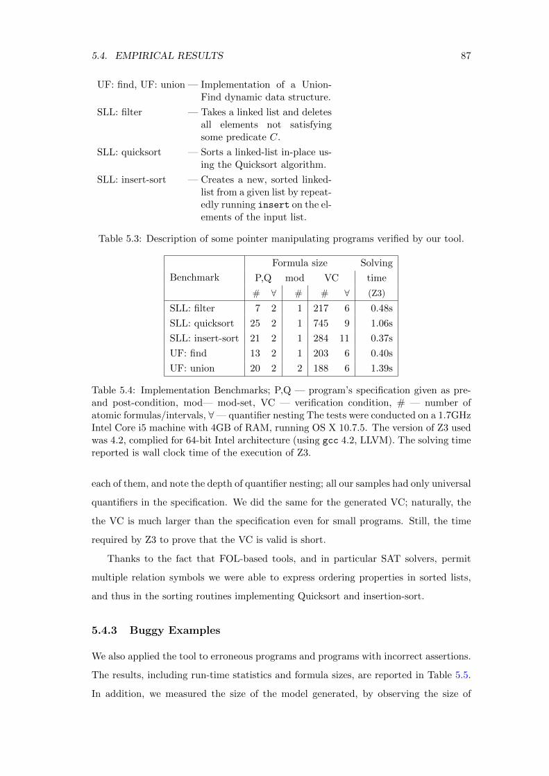
5.4. EMPIRICAL RESULTS 87
UF: find, UF: union — Implementation of a Union-Find dynamic data structure.
SLL: filter — Takes a linked list and deletesall elements not satisfyingsome predicate C.
SLL: quicksort — Sorts a linked-list in-place us-ing the Quicksort algorithm.
SLL: insert-sort — Creates a new, sorted linked-list from a given list by repeat-edly running insert on the el-ements of the input list.
Table 5.3: Description of some pointer manipulating programs verified by our tool.
Benchmark
Formula size Solving
P,Q mod VC time
# ∀ # # ∀ (Z3)
SLL: filter 7 2 1 217 6 0.48s
SLL: quicksort 25 2 1 745 9 1.06s
SLL: insert-sort 21 2 1 284 11 0.37s
UF: find 13 2 1 203 6 0.40s
UF: union 20 2 2 188 6 1.39s
Table 5.4: Implementation Benchmarks; P,Q — program’s specification given as pre-and post-condition, mod— mod-set, VC — verification condition, # — number ofatomic formulas/intervals, ∀— quantifier nesting The tests were conducted on a 1.7GHzIntel Core i5 machine with 4GB of RAM, running OS X 10.7.5. The version of Z3 usedwas 4.2, complied for 64-bit Intel architecture (using gcc 4.2, LLVM). The solving timereported is wall clock time of the execution of Z3.
each of them, and note the depth of quantifier nesting; all our samples had only universal
quantifiers in the specification. We did the same for the generated VC; naturally, the
the VC is much larger than the specification even for small programs. Still, the time
required by Z3 to prove that the VC is valid is short.
Thanks to the fact that FOL-based tools, and in particular SAT solvers, permit
multiple relation symbols we were able to express ordering properties in sorted lists,
and thus in the sorting routines implementing Quicksort and insertion-sort.
5.4.3 Buggy Examples
We also applied the tool to erroneous programs and programs with incorrect assertions.
The results, including run-time statistics and formula sizes, are reported in Table 5.5.
In addition, we measured the size of the model generated, by observing the size of

88 CHAPTER 5. MODULAR ANALYSIS OF PROCEDURES
Formula size Solving C.e.
Benchmark P,Q VC time size
(+ Nature of de-
fect)
# ∀ # ∀ (Z3) (|L|)
UF: find 27 3 201 6 1.60s 2
Incorrect handling
of corner case
UF: union 19 2 186 6 0.70s 8
Incorrect specifica-
tion
SLL: filter 36 4 317 6 0.49s 14
Uncontrolled shar-
ing
SLL: insert-sort 21 2 283 9 0.88s 8
Unmet call precon-
dition
Table 5.5: Information about benchmarks that demonstrate detection of several kinds ofbugs in pointer programs. In addition to the previous measurements, the last columnlists the size of the generated counterexample in terms of the number of vertices —linked-list or tree nodes.
the generated domain—which reflects the number of nodes in the heap. As expected,
Z3 was able to produce concrete counterexamples of reasonable size, providing output
that is readable for the programmer and useful for debugging. Since these are slight
variations of the correct programs, size and running time statistics are similar.
5.5 Related Work for Chapter 5
Modular Verification. The area of modular procedure specification is heavily stud-
ied. Many of these works require that the user declare potential changes similar to
the modset (e.g., see [4, 41, 66, 71]). The frame rule of separation logic [35] naturally
supports modular reasoning where the separating conjunction combines the local post-
condition with the assertion at the call site. Unlike separation, reachability is a higher
abstraction which relies on type correctness and naturally abstracts operations such
as garbage collection. Nevertheless, in Section 6.2 we show that it can also deal with
explicit memory reclamations.
We believe that our work pioneers the use of an effectively propositional logic, which
is a weak logical fragment, to perform modular reasoning in a sound and complete way.

5.5. RELATED WORK FOR CHAPTER 5 89
Our adaptation rule is more complex than the frame rule as it automatically updates
reachability.
Cutpoints. Rinetzky et al. [56] introduce cutpoint objects which are objects that can
reach the area of the heap accessible by the procedure without passing through objects
directly pointed-to by parameters. Cutpoints complicate program reasoning. They are
used in model checking [1] and static analysis [24, 57]. Examples such as the ones in
[58] which include (unbounded) cutpoints from the stack are handled by our method
without any changes. These extra cutpoints cannot change the reachabilty and thus
have no effect. Interestingly, we can also handle certain programs which manipulate
unbounded cutpoints. Instead, we do limit the amount of new sharing in paths which
are necessary for the verification. For example, the find procedure shown in Fig. 5.2
includes unbounded sharing which can be created by the client program. A typical
client such as a spanning tree construction algorithm will indeed create unbounded
sharing. In the future, we plan to verify such clients by abstracting away the pointers
inside the union-find tree.

Chapter 6
Discussion
6.1 On the Expressivity Limitations of AFR
6.1.1 Inversion yielding a non-AFR formula
We show here that a naıve attempt to encode the summary of a procedure (e.g. the
one in Fig. 3.1) immediately leads to formula that are not AFR.
Take I ′9 (Eq (3.3)), and substitute occurrences of 〈n〉 using the inversion formula
Eq (3.6). We obtain—
∀α, β :(α〈n+〉β ∧ ∀γ : α〈n+〉γ → β〈n∗〉γ
)⇔(
α〈n+0 〉β ∧ ∀γ : α〈n+
0 〉γ → β〈n∗0〉γ)
which, when converted to Prenex normal form yields the non-AFR formula
∀α, β : ∃γ1∀γ′1 ∃γ2∀γ′2 :(α〈n+〉β ∧ (α〈n+〉γ1 → β〈n∗〉γ1)→
α〈n+0 〉β ∧ (α〈n+
0 〉γ′1 → β〈n∗0〉γ′1))
∧(α〈n+
0 〉β ∧ (α〈n+0 〉γ2 → β〈n∗0〉γ2)→
α〈n+〉β ∧ (α〈n+〉γ′2 → β〈n∗〉γ′2))
6.1.2 Formulas not expressible in AFR
Unbounded cutpoints. In Section 3.2 we saw that with the assumption of owner-
ship, the postcondition of reverse could be expressed as an AFR formula. In contrast,
90

6.1. ON THE EXPRESSIVITY LIMITATIONS OF AFR 91
void correl_lists(int sz) {Node c = null; Node d = null;
while (sz > 0) {Node t = new Node();
t.next = c; c = t;
t = new Node();
t.next = d; d = t;
}while (c != null) {c = c.next;d = d.next;
}}
Figure 6.1: A simple Java program that creates two correlated lists.
if we assume an unbounded number of cutpoints then Eq (3.10) must be changed to
∀α, β : α〈n∗〉β ⇔
β〈n∗0〉α h0〈n∗0〉α ∧ h0〈n∗0〉β
α〈n∗0〉β ¬h0〈n∗0〉α ∧ ¬h0〈n∗0〉β
false h0〈n∗0〉α ∧ ¬h0〈n∗0〉β
∃γ : α〈n∗0〉γ ∧
¬h0〈n∗0〉γ ∧ β〈n∗0〉n0(γ)
¬h0〈n∗0〉α ∧ h0〈n∗0〉β
(6.1)
The first three cases are the same as in Eq (3.10). The last case considers the situation
where α is outside the list while β is within the list. For α to reach β in the postcon-
dition, it must be the case that there exists a node γ such that γ is outside the list but
its successor is within the list and reachable from β. The formula, however, introduces
alternation of ∃ inside ∀ and the use of the function symbol n so it is outside AER (and
thus outside AFR).
Correlations Between Data Structures. Another example of a non-AFR formula
mentioned concerns programs that manipulate two lists of the same length. The pro-
gram in Fig. 6.1 demonstrates a case where a weak logic is not enough to prove the
absence of null dereference in a pointer program. The first while loop creates two lists
of length sz. Then, taking advantage of the equal lengths, it traverses the first list —
the one pointed to by c — while at the same time advancing the pointer d.
92 CHAPTER 6. DISCUSSION
Since each iterator advances one step, the second loop preserves an invariant that the
lists at c and d are of the same length. Hence, as long as c is not null, it guarantees that
d is not null either. Unfortunately, such an invariant requires an inductive definition
which is well outside of AFR:
eqlen(x, y)def= (x = null ∧ y = null) ∨(
x 6= null ∧ y 6= null ∧ eqlen(n(x),n(y)))
6.2 Extensions
Doubly-linked List and Nested Lists. To verify a program that manipulates a
doubly-linked list, all that needs to be done is to duplicate the analysis we did for n,
for a second pointer field prev. As long as the only atomic formulas used in assertions
are α〈n∗〉β and α〈prev∗〉β (and not, for example, α〈(n|prev)∗〉β), providing the substi-
tutions for atomic formulas in Table 3.3 would not get us outside of the class AER. In
particular, we have verified the doubly-linked list property:
∀α, β : h〈n∗〉α ∧ h〈n∗〉β =⇒ (α〈n∗〉β ⇔ β〈prev∗〉α).
In fact we can verify nested lists and, in general, lists with arbitrary number of pointer
fields as long as reachability constraints are expressed using only one function symbol
at a time, like in the case of next and prev above.
Cycles. For data structures with a single pointer, the acyclicity restriction may be
lifted by using an alternative formulation that keeps and maintains more auxiliary
information [28, 40]. Instead of keeping track of just n∗, we instrument the edge addition
operation with a check: if the added edge is about to close a cycle, then instead of adding
the edge, we keep it in a separate set M of “cycle-inducing” edges. Two properties of
lists now come into play: (1) The number of cycles reachable from program variables,
and hence the size of M , is bounded by the number of program variables; (2) Any
path (simple or otherwise) in the heap may utilize at most one of those edges, because
once a path enters a cycle, there is no way out. In all assertions, therefore, we replace
α〈n∗〉β with: α〈n∗〉β∨∨〈u,v〉∈M (α〈n∗〉u∧v〈n∗〉β). Notice that it is possible to construct

6.2. EXTENSIONS 93
All lists are acyclic sll(n∗) ∧ sll(m∗)
No sharing between lists∀α, β, γ : h〈n∗〉α ∧ α〈m∗〉β ∧
h〈n∗〉γ ∧ γ〈m∗〉β =⇒ α = γ
Hierarchy ∀α, β, γ : α 6= β ∧ β 6= γ ∧ α〈m∗〉β =⇒ ¬β〈n∗〉γ
Cycle edge∀α, β, γ : α 6= β ∧ α 6= γ ∧ α〈n∗〉β =⇒ ¬α〈c〉γ∀α, β : β〈c〉α =⇒ h〈n∗〉α ∧ α〈m∗〉β
Table 6.1: Properties of a list of cyclic lists expressed in AFR
this formula thanks to the bound on the size of M ; otherwise, an existential quantifier
would have been required in place of the disjunction.
Cycles can also be combined with nesting, in such a way as to introduce an un-
bounded number of cycles. To illustrate this, consider the example of a linked list
beginning at h and formed by a pointer field which we shall denote n, where each el-
ement serves as the head of a singly-linked cycle along a second pointer field m. This
is basically the same as in the case of acyclic nested lists, only that the last node in
every sub-chain (a list segment formed by m) is connected to the first node of that
same chain.
One way to model this in a simple way is to assume that the programmer designates
the last edge of each cycle; that is, the edge that goes back from the last list node to
the first. We denote this designation by introducing a ghost field named c. This
cycle-inducing edge is thus labeled c instead of m.
Properties of the nested data structure can be expressed with AFR formulas as
shown in Table 6.1. “Hierarchy” means that the primary list is contiguous, that is,
there cannot be n-pointers originating from the middle of sub-lists. “Cycle edge”
describes the closing of the cyclic list by a special edge c.
We were able to verify the absence of memory errors and the correct functioning of
the program flatten, shown in Fig. 6.2.
Bounded Sharing. Arbitrary sharing in data structures is hard, because even in
lists, any node of the list may be shared (that is, have more than one incoming edge).
In this case we have to use quantification since we do not know in advance which node
in the list is going to be a cutpoint for which other nodes. However, when the entire
heap consists solely of lists, the quantifier may be replaced with a disjunction if we take
into account that there is a bounded number of program variables, which can serve

94 CHAPTER 6. DISCUSSION
Node flatten(Node h) {Node i = h, j = null;
while (i != null) I1 {Node k = i;
while (k != null) I2 {j = k; k = k.m;
}j.c = null;
i = i.n; j.m = null; j.m = i;
}j.c = null; j.c := h;
return h;
}
Figure 6.2: A program that flattens a hierarchical structure of lists into a single cycliclist.
Command Pre Mod Post
ret = new() free(s) ∅ ret = s ∧ ¬free(s)
access y ¬free(y) ∅free(y) y 6= null ∧ ¬free(y) ∅ free(y)
Table 6.2: The specifications of atomic commands for resource allocations in a C-likelanguage.
as the heads of lists, and any two lists have at most one cutpoint. Such heaps when
viewed as graphs are much simpler than general DAGs, since one can define in advance
a set of constant symbols to hold the edges that induce the sharing; for example, if we
have one list through the nodes x→ u1 → u2 and a second list through y → v1 → v2,
all distinct locations, then adding an edge u2 → v1 would create sharing, as the nodes
v1, v2 become accessible from both x and y. This technique is also covered by Hesse [28].
Explicit Memory Management Table 6.2 updates the specification of atomic com-
mands (provided in Table 5.1) to handle explicit memory management operations. For
simplicity, we follow ANSI C semantics but do not handle arrays and pointer arithmetic.
The allocation statement assigns a freed location denoted by s to ret and sets its value
to be non-freed. All accesses to memory locations pointed-to by y in statements ret =
y.f, y.f = x, and x = y are required to access non-freed memory. Finally, free(y)
sets the free predicate to true for the node pointed-to by y. As a result, all the nodes
reachable from y cannot be accessed.
Notice that it is possible to enforce interesting safety properties naturally using
6.2. EXTENSIONS 95
AFR formulas such as the absence of memory leaks. For example a precondition for
free(x) can be
∀α : y〈f∗〉α ∧ α 6= y ∧ α 6= null→ free(y)

Chapter 7
Conclusion
In this thesis we investigated complex properties of programs, involving high-order
concepts as transitive closure of pointer links and its derivatives such as sharing and
entry-point. It is surprising that such properties can be expressed and handled by a
logic based on EPR, which is among the weakest fragments of first-order logic. A key
insight to enable this was the idea of “inversion”: instead of a function symbol for next
and a derived binary relation next∗ for its transitive closure, formalize the properties
of next∗ and have next derived from it instead. As previously noted, this is analogous
to reasoning in the natural numbers using a successor function succ (which requires
constant use of induction) vs. reasoning with ≤.
The results shed some light on the complexity of reasoning about programs that
manipulate linked data structures such as singly- and doubly-linked lists. The invariants
in many of these programs can be expressed without quantifier alternation. Alternations
are introduced by unbounded cutpoints and reasoning about more complicated directed
acyclic graphs. Furthermore, for programs manipulating general graphs higher order
reasoning may be required.
Compared to past work on shape analysis, our approach (i) is based on full predicate
abstraction, (ii) makes use of standard theorem proving techniques, (iii) is capable of
reporting concrete counterexamples, and (iv) is based on property-directed reachability.
The experimental evaluation in Section 4.3 illustrates these four advantages of our
approach. The algorithm is able to establish memory-safety and preservation of data-
structure invariants for all of the examples, using only a handful of simple predicates.
This result may look somewhat surprising because earlier work on shape analysis that
employed the same predicates [26] failed to prove these properties. One reason is
96
97
that [26] only uses positive and negative combinations of these predicates, whereas our
algorithm uses arbitrary Boolean combinations of predicates.
A crucial method for simplifying the reasoning about linked data structures is par-
titioning programs into smaller pieces, where each piece manipulates part of the heap.
The part that a sub-program manipulate usually has a bounded number of entry and
exit points. This thesis slightly generalizes by reasoning about a potentially unbounded
number of entry points, as demonstrated by find and union. Only the new sharing
that is introduced by the procedure should be bounded. Notice that this unbounded-
ness supports modularity: even in the case where in every particular call context there
is a bounded number of paths (e.g. when there is a bounded number of roots in the
heap), the bound is not known in advance, therefore the programmer has to prepare
for an unbounded number of cases.
It is important to note that the adaptation rule of Section 5.2 adds expressive power
to verifying programs: it is in general impossible for the programmer to define, in AFR,
a modular specification for all the procedures. Generation of a verification condition
requires coordination between the separate call sites as mentioned above, in particular
taking note of potential sharing. This coordination requires per-call-site instantiation,
which, thanks to having the adaptation rule in the framework, is done automatically.
Finally we remark that there is a trade-off between the complexity of the mod-set
and of the post-condition: defining a simpler, but larger mod may cause the post-
condition to become more complicated, sometimes not even AFR-expressible. Also
notice that if mod = V (the entire heap), modular reasoning becomes trivial since it
can be done by relational composition, but this puts the burden of writing the most
complete post-conditions on the programmer, which we suspect is not always possible
in our limited logic.
Therefore, we believe that this thesis is an important step towards the ability to
handle real-life programs in a scalable way.
There are some issues still open. As we have seen, there is an interesting class of
programs that work on linked data structures with pointers and admit EPR induc-
tive loop invariants. Since EPR is a countable set of formulas, and from the decision
procedure developed in the previous chapters, the problem of checking whether a pro-
gram has such a loop invariant becomes r.e. by a simple generate-and-test approach
(of course, in general, the problem of checking a single loop invariant is undecidable,

98 CHAPTER 7. CONCLUSION
and the problem of finding a loop invariant is not r.e.). Is there a better way to an-
swer this question? The method represented in Chapter 4 for invariant inference allows
limited use of quantifiers, restricted by the parameter templates. It would be useful
to learn new quantified predicates and refine the abstractions (e.g. using CEGAR);
this would require less from the programmer and would allow more instances where
fully-automated reasoning on loops can be applied. On a broader scale, we raise a
theoretical question of whether an EPR invariant can be discovered automatically, and
whether the existence of an EPR invariant is decidable. We conjecture, however, that
the answer would be negative, although a proof is yet to be discovered.
The solution might be a heuristic for EPR inductive loop invariant inference that
would be sound but not complete; while not providing a conclusive solution, a heuristic
has a high chance of working well in practice because naturally-occurring programs
are usually “well-behaved” and have a simple argument that proves their correctness.
Moreover, it can be argued that having a simple loop invariant is a good programming
trait by its own right and that programmers should make an effort to write such pro-
grams. In any case, it is obvious that the programs presented in undecidability proofs
are highly unnatural and there is no practical need to handle such instances.
To design such heuristics, a larger base of benchmarks should be obtained and
inspected to characterize what common programming idioms exist, then exploit prop-
erties of these idioms to handle variants of the benchmarks in different contexts.
On the aspects of modular programming and reasoning, we still do not know the
bounds of modular reasoning and in which situations it can be used. The restriction of
bounded sharing (Section 5.3.2.4) may be too severe for some cases, and can probably be
avoided. Also, it is interesting to investigate the differences and similarities of handling
procedure calls within loops vs. handling recursion as is done in this thesis.
Finally, the success we had with reasoning of transitive closure gives hope that this
kind of reasoning can also be applied for the field of synthesis, where invariants are
given and the code is automatically generated, rather than being checked against the
specifications. This can be a win-win situation, since sometimes generation of code
may even be easier than verification, and the resulting code is correct by construction.

Appendix A
Logical Proofs
Definition 15 (Vocabulary). A vocabulary V is a triple 〈C,F ,R〉 where C is a finite
set of constant symbols, F is a finite set of function symbols where each f ∈ F has a
fixed arity ar(f), and R is a finite set of relation symbols where each r ∈ R has a fixed
arity ar(r).
A.1 Reductions between Logics
We now state the reduction from the problem of checking validity of an AER formula
to effectively-propositional logic for a specific function n. It can be generalized for any
fixed number of function symbols in order to handle, for example, doubly-linked lists
or nested lists. First we show that for acyclic functions over finite domains, there is a
one-to-one correspondence between n and n∗, as hinted previously by Eq (3.6).
Let L be the set of memory locations (“objects”). Let α ∈ L be some node, then
the set of nodes reachable from α, that is, W = {β | α〈n∗〉β}, is linearly ordered via
n∗. Thus α has a unique successor — namely, the minimal node of W \{α}. This gives
rise to the following lemma:
Lemma 3. For n : L→ L ∪ {null}, which is acyclic,
β = n(α) ⇐⇒ α〈n+〉β ∧ ∀γ : α〈n+〉γ =⇒ β〈n∗〉γ
for any α, β ∈ L.
Proof. First direction (⇒): Let β = n(α). Trivially α〈n+〉β. Assume some γ ∈ L such
that α〈n+〉γ, then n(α)〈n∗〉γ; Hence β〈n∗〉γ.
99

100 APPENDIX A. LOGICAL PROOFS
Second direction (⇐): Let α〈n+〉β and α〈n+〉γ =⇒ β〈n∗〉γ for any γ ∈ L. From
the first clause, n(α)〈n∗〉β. From the second, since α〈n+〉n(α), follows β〈n∗〉n(α). Due
to acyclicity, β = n(α).
Relying on the fact that L is finite, the right-hand side of the lemma necessarily
defines a total function (which is, in fact, computable). We can use this fact to simulate
reachability constraints in first-order logic. For this purpose, we use the formula ϕ′ from
Eq (3.7) (Section 3.2).
Proposition 2 (Simulation of AER) Consider an AER formula ϕ over vocabulary
V = 〈C, {n},R〉. Let ϕ′ def= ϕ[n∗(t1, t2)/t1〈n∗〉t2]. Then ϕ′ is a FO formula over vocab-
ulary V ′ = 〈C, ∅,R∪ {n∗}〉 and ϕ is simulated by ΓlinOrd → ϕ′ where ΓlinOrd is the
formula in Table 3.2.
Proof. We need to show that ϕ is valid ⇐⇒ ϕ′ is valid.
First direction (⇒): Suppose that ϕ is true on all appropriate structures. Let
A′ ∈ STRUC(V ′) be an arbitrary finite structure for ϕ′, with domain L such that
A′ |= ΓlinOrd. Define nA as in Lemma 3 — this is well-defined since L is finite. We got
a structure A for ϕ, so A |= ϕ, and (nA)∗ = n∗A′
. Therefore, A′ |= ϕ′.
Second direction (⇐): Conversely, suppose that ΓlinOrd =⇒ ϕ′ is true on all
appropriate structures, and let A ∈ STRUC(V) be an arbitrary structure for ϕ; By
setting n∗A′
= (nA)∗ we get A′, which is a model of ΓlinOrd; hence from the assumption,
A′ |= ϕ′; therefore A |= ϕ.
A.2 Program Semantics
This section of the appendix refers to the definitions of Table 2.2, Table 2.3 (Section 2.2)
and Table 3.3 (Section 3.4).
Proposition 3 (VCs in AER) For every program S whose precondition P , postcon-
dition Q, branch conditions, loop conditions, and loop invariants are all expressed as
AFR formulas, VCgen({P}S{Q}) ∈ AER.
Proof. Follows from closure properties of AER, and from the fact that AER is closed
under wlp, The proofs of which immediately follow. In particular, in VCaux(while . . .),
the subformulas [[B]] and I are AFR and Q is AER. Thus I∧[[B]]→ Q is AER. Similarly
for the ¬[[B]] case.

A.2. PROGRAM SEMANTICS 101
The following proposition summarizes the properties of formulas which are used to
guarantee that we can generate AFR formulas for arbitrary procedures manipulating
singly and doubly linked lists with AFR specified invariants.
Proposition 8 (Closure of AER Formulas). Let af be a closed AFR formula, qf be a
QFR formula. Let ϕ1 and ϕ2 be closed AER formulas. Let a be an atomic subformula in
ϕ1 and let ϕ1[qf/a] denote the substitution of a in ϕ1 by qf. Let c be a constant. Then,
the following formulas are all AER formulas: disjunction: ϕ1∨ϕ2; conjunction: ϕ1∧ϕ2; AFR-implication: af =⇒ ϕ1; QFR-substitution: ϕ1[qf/a]; generalization:
∀α : ϕ1[α/c].
Theorem 5. (Soundness and Completeness of the wlp rules for heap
access—atomic statements) For every state σ be a structure with the vocabulary
〈Pvar, {n},R〉 over a set of locations L, for every atomic heap access atomic statement
S, σ |= wlp[[S]](Q) if and only if [[S]]σ |= Q ∧ ac.
Proof. We will prove the theorem in terms of the operational semantics of the atomic
statements.
Let σ, σ′ ∈ Σ be program states such that σ |= P ∧ ac.So nσ is a function without cycles.
Consider the two atomic commands whose semantics update n — this is based
almost completely on [28]:
S = x.n := y: Assume that nσ(xσ) = null. Then n[[S]]σ(xσ) = yσ, and for any α 6= xσ,
n[[S]]σ(α) = nσ(α). In this case, α〈n[[S]]σ∗〉β ⇐⇒ α〈nσ∗〉β ∨ (α〈nσ∗〉xσ ∧ yσ〈nσ∗〉β), so
via our assumption,
[[S]]σ |= Q ⇐⇒ σ |= Q[α〈n∗〉β ∨ (α〈n∗〉x ∧ y〈n∗〉β)/α〈n∗〉β)]
Because σ and [[S]]σ differ only in n (values of all program variables are the same), that
is [[S]]σ = σ[n 7→ n[[S]]σ].
S = x.n := null: Similarly, we have n[[S]]σ(xσ) = null and for any α 6= xσ, n[[S]]σ(α) =
nσ(α). Therefore in this case α〈n[[S]]σ∗〉β ⇐⇒ α〈nσ∗〉β∧(¬α〈nσ∗〉xσ∨β〈nσ∗〉xσ) (here
it is important that we know that n is without cycles). Hence,
[[S]]σ |= Q ⇐⇒ σ |= Q[α〈n∗〉β ∧ (¬α〈n∗〉x ∨ β〈n∗〉x)/α〈n∗〉β]
102 APPENDIX A. LOGICAL PROOFS
Consider the atomic command whose semantics read the value of n. These do not
change n, so safely σ |= ac ⇐⇒ [[S]]σ |= ac. It is left to check the condition for Q:
S = x := y.n: Assume ` ∈ L such that σ,A |= Pn[y/s, α/t] where A = [α 7→ `] is
a variable assignment for a fresh variable a. According to Lemma 3, this means that
nσ(yσ) = `. We then get [[S]]σ = σ[x 7→ nσ(yσ)] = σ[x 7→ `].
[[S]]σ |= Q ⇐⇒ σ[x 7→ `] |= Q ⇐⇒ σ,A |= Q[α/x]
And since this holds for any A as above,
[[S]]σ |= Q ⇐⇒ σ |= ∀α : Pn[y/s, α/t] =⇒ Q[α/x]
Finally, consider the atomic command that allocates memory.
S = x := new: We model the memory allocation as a function M : Σ→ L that given a
structure σ, returns a non-null location ` ∈ L such that ` is not “used” — in the sense
that it cannot be reached from any of the program variables, that is, constant symbols
of the set Pvar. In this case [[S]]σ = σ[x 7→M(σ)]. Also,
σ,[α 7→M(σ)
]|=
∧p∈Pvar∪{null}
¬p〈n∗〉α
Assume σ |= ∀α :(∧
p∈Pvar∪{null} ¬p〈n∗〉α)
=⇒ Q[α/x]. Hence from the use of
∀, we know that σ,[α 7→ M(σ)
]|=(∧
p∈Pvar∪{null} ¬p〈n∗〉α)
=⇒ Q[α/x]. Combined
with M specifications, σ,[α 7→M(σ)
]|= Q[α/x]. Hence [[S]]σ |= Q.
Now assume that [[S]]σ |= Q. It means it should hold for any implementation of M .
Let ` = M(σ), then we know that ` can be any location such that
σ,A |=∧
p∈Pvar∪{null}¬p〈n∗〉α
Where A =[α 7→ `]. Also, σ,A |= Q[α/x] from the same reasons as before. Since
this holds for any such A satisfying the antecendant, we conclude that σ |= ∀α :(∧p∈Pvar∪{null} ¬p〈n∗〉α
)=⇒ Q[α/x].
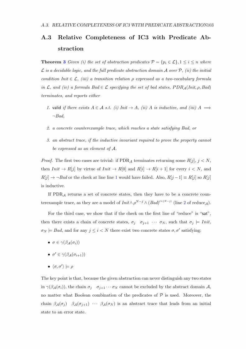
A.3. RELATIVE COMPLETENESS OF IC3WITH PREDICATE ABSTRACTION103
A.3 Relative Completeness of IC3 with Predicate Ab-
straction
Theorem 3 Given (i) the set of abstraction predicates P = {pi ∈ L}, 1 ≤ i ≤ n where
L is a decidable logic, and the full predicate abstraction domain A over P, (ii) the initial
condition Init ∈ L, (iii) a transition relation ρ expressed as a two-vocabulary formula
in L, and (iv) a formula Bad ∈ L specifying the set of bad states, PDRA(Init, ρ,Bad)
terminates, and reports either
1. valid if there exists A ∈ A s.t. (i) Init→ A, (ii) A is inductive, and (iii) A =⇒¬Bad,
2. a concrete counterexample trace, which reaches a state satisfying Bad, or
3. an abstract trace, if the inductive invariant required to prove the property cannot
be expressed as an element of A.
Proof. The first two cases are trivial: if PDRA terminates returning some R[j], j < N ,
then Init → R[j] by virtue of Init → R[0] and R[i] → R[i + 1] for every i < N , and
R[j]→ ¬Bad or the check at line line 1 would have failed. Also, R[j−1] ≡ R[j] so R[j]
is inductive.
If PDRA returns a set of concrete states, then they have to be a concrete coun-
terexample trace, as they are a model of Init∧ ρN−j ∧ (Bad)′×(N−j) (line 2 of reduceA).
For the third case, we show that if the check on the first line of “reduce” is “sat”,
then there exists a chain of concrete states, σj σj+1 · · · σN , such that σj |= Init,
σN |= Bad, and for any j ≤ i < N there exist two concrete states σ, σ′ satisfying:
• σ ∈ γ(βA(σi))
• σ′ ∈ γ(βA(σi+1))
• 〈σ, σ′〉 |= ρ
The key point is that, because the given abstraction can never distinguish any two states
in γ(βA(σi)), the chain σj σj+1 · · ·σN cannot be excluded by the abstract domain A,
no matter what Boolean combination of the predicates of P is used. Moreover, the
chain βA(σj) βA(σj+1) · · · βA(σN ) is an abstract trace that leads from an initial
state to an error state.

104 APPENDIX A. LOGICAL PROOFS
Notice that the chain above may not be a concrete trace, there can be “breaks”
between adjacent σis, within the same abstract element.
Construction of (σi)i=j...N : Follow the chain of recursive calls to “reduce” with
index values N down to j. The parameter A is always a cube of the form βA(σ);
take one σ |= A for each call, forming a series that we denote by σj , σj+1, etc. We
show that this series satisfies the above properties: At each call except the innermost,
“reduce” made a recursive call at line 7, which means that R[j − 1] ∧ ρ ∧ (A)′ was
satisfiable; the returned cube A2 becomes βA(σj−1). Let 〈σ, σ′〉 |= R[j − 1] ∧ ρ ∧ (A)′,
then σ |= A2 = βA(σj−1); σ′ |= A = βA(σj); and 〈σ, σ′〉 |= ρ as required.
A.4 Simulation of an Idempotent Function in EPR
We prove Theorem 4, by providing a concrete translation in three steps. First, we
translate ϕ to a ∀∗∃∗-formula ϕ′ as described in Proposition 2, keeping the function
symbols g, h1, . . . , hn as is. Similarly to the proof of Proposition 2, one obtains that
(a) if ϕ is valid in all finite structures then ϕ′ is valid in all finite structures; and (b) if
ϕ′ is valid then ϕ is valid.
Second, to eliminate the function symbols h1, . . . , hn we repetitively use the follow-
ing proposition:
Proposition 9. Let N > 0. Let h be some unary function symbol, and Σh be
a first-order signature (with equality) that includes the function symbol h. Let ΣR
be the signature obtained from Σh by replacing h with a binary relation symbol Rh,
and adding N fresh constant symbols c1, . . . , cN . Consider an ∃∗∀∗ sentence over
Σg: Φ = ∃x1, . . . , xn.∀y1, . . . , ym.Ψ (where Ψ is quantifier free, over the variables
x1, . . . , xn, y1, . . . , ym). Suppose that the only terms occurring in Φ that involve h have
the form h(z), where z is a variable. Define T (Φ) to be the following sentence over ΣR:
Γ ∧ ∃x1, xh1 , . . . , xn, xhn.∀y1, yh1 , . . . , ym, yhm.∧1≤i≤nRh(xi, x
hi ) ∧ (
∧1≤i≤mRh(yi, y
hi )→ Ψ′)
(A.1)
where:
• Γ is the conjunction of the following formulas:
– ∀x, y, z.Rh(x, y) ∧Rh(x, z)→ y = z
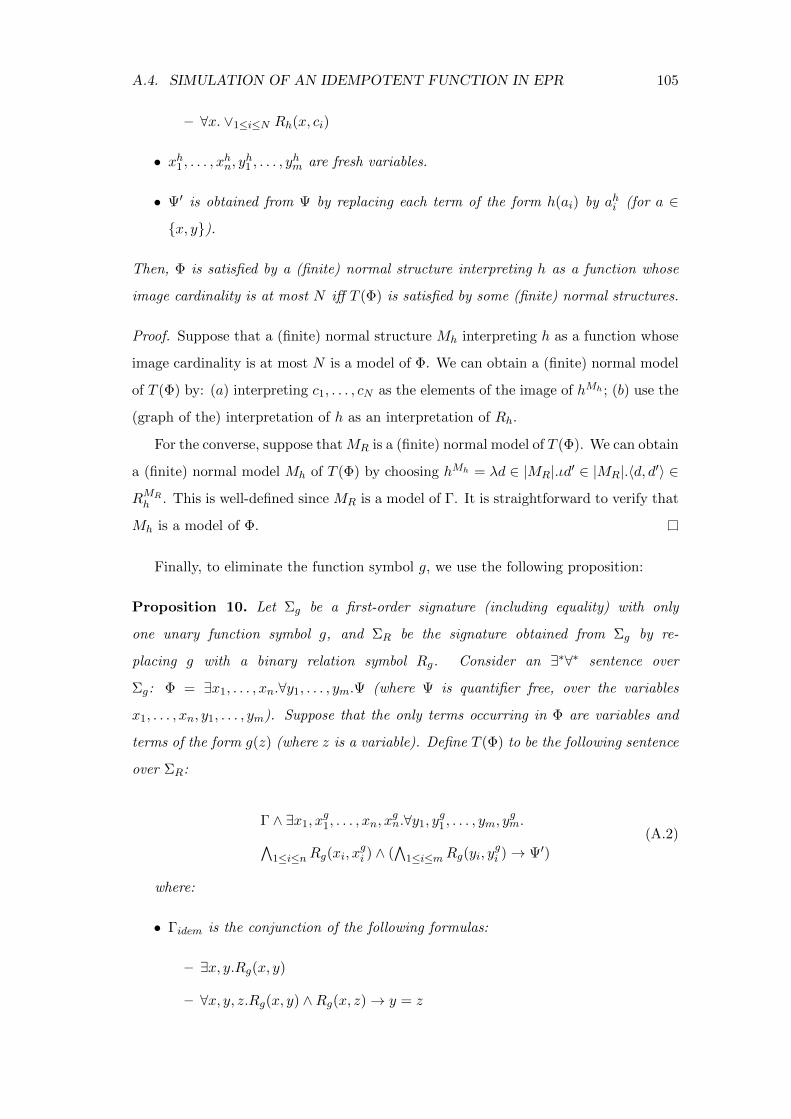
A.4. SIMULATION OF AN IDEMPOTENT FUNCTION IN EPR 105
– ∀x. ∨1≤i≤N Rh(x, ci)
• xh1 , . . . , xhn, yh1 , . . . , yhm are fresh variables.
• Ψ′ is obtained from Ψ by replacing each term of the form h(ai) by ahi (for a ∈{x, y}).
Then, Φ is satisfied by a (finite) normal structure interpreting h as a function whose
image cardinality is at most N iff T (Φ) is satisfied by some (finite) normal structures.
Proof. Suppose that a (finite) normal structure Mh interpreting h as a function whose
image cardinality is at most N is a model of Φ. We can obtain a (finite) normal model
of T (Φ) by: (a) interpreting c1, . . . , cN as the elements of the image of hMh ; (b) use the
(graph of the) interpretation of h as an interpretation of Rh.
For the converse, suppose thatMR is a (finite) normal model of T (Φ). We can obtain
a (finite) normal model Mh of T (Φ) by choosing hMh = λd ∈ |MR|.ιd′ ∈ |MR|.〈d, d′〉 ∈RMRh . This is well-defined since MR is a model of Γ. It is straightforward to verify that
Mh is a model of Φ.
Finally, to eliminate the function symbol g, we use the following proposition:
Proposition 10. Let Σg be a first-order signature (including equality) with only
one unary function symbol g, and ΣR be the signature obtained from Σg by re-
placing g with a binary relation symbol Rg. Consider an ∃∗∀∗ sentence over
Σg: Φ = ∃x1, . . . , xn.∀y1, . . . , ym.Ψ (where Ψ is quantifier free, over the variables
x1, . . . , xn, y1, . . . , ym). Suppose that the only terms occurring in Φ are variables and
terms of the form g(z) (where z is a variable). Define T (Φ) to be the following sentence
over ΣR:
Γ ∧ ∃x1, xg1, . . . , xn, xgn.∀y1, yg1 , . . . , ym, ygm.∧1≤i≤nRg(xi, x
gi ) ∧ (
∧1≤i≤mRg(yi, y
gi )→ Ψ′)
(A.2)
where:
• Γidem is the conjunction of the following formulas:
– ∃x, y.Rg(x, y)
– ∀x, y, z.Rg(x, y) ∧Rg(x, z)→ y = z
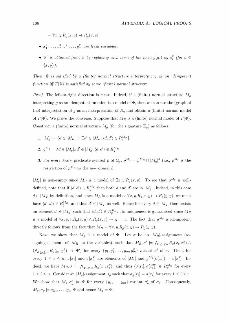
106 APPENDIX A. LOGICAL PROOFS
– ∀x, y.Rg(x, y)→ Rg(y, y)
• xg1, . . . , xgn, yg1 , . . . , ygm are fresh variables.
• Ψ′ is obtained from Ψ by replacing each term of the form g(ai) by agi (for a ∈{x, y}).
Then, Φ is satisfied by a (finite) normal structure interpreting g as an idempotent
function iff T (Φ) is satisfied by some (finite) normal structure.
Proof. The left-to-right direction is clear. Indeed, if a (finite) normal structure Mg
interpreting g as an idempotent function is a model of Φ, then we can use the (graph of
the) interpretation of g as an interpretation of Rg and obtain a (finite) normal model
of T (Φ). We prove the converse. Suppose that MR is a (finite) normal model of T (Φ).
Construct a (finite) normal structure Mg (for the signature Σg) as follows:
1. |Mg| = {d ∈ |MR| : ∃d′ ∈ |MR|.〈d, d′〉 ∈ RMRg }
2. gMg = λd ∈ |Mg|.ιd′ ∈ |Mg|.〈d, d′〉 ∈ RMRg
3. For every k-ary predicate symbol p of Σg, pMg = pMR ∩ |Mg|k (i.e., pMg is the
restriction of pMR to the new domain).
|Mg| is non-empty since MR is a model of ∃x, y.Rg(x, y). To see that gMg is well-
defined, note that if 〈d, d′〉 ∈ RMRg then both d and d′ are in |Mg|. Indeed, in this case
d ∈ |Mg| by definition, and since MR is a model of ∀x, y.Rg(x, y)→ Rg(y, y), we must
have 〈d′, d′〉 ∈ RMRg , and thus d′ ∈ |Mg| as well. Hence for every d ∈ |Mg| there exists
an element d′ ∈ |Mg| such that 〈d, d′〉 ∈ RMRg . Its uniqueness is guaranteed since MR
is a model of ∀x, y, z.Rg(x, y) ∧ Rg(x, z) → y = z. The fact that gMg is idempotent
directly follows from the fact that MR |= ∀x, y.Rg(x, y)→ Rg(y, y).
Now, we show that Mg is a model of Φ. Let σ be an |MR|-assignment (as-
signing elements of |MR| to the variables), such that MR, σ′ |= ∧
1≤i≤nRg(xi, xgi ) ∧
(∧
1≤i≤mRg(yi, ygi ) → Ψ′) for every {y1, yg1 , . . . , ym, ygm}-variant σ′ of σ. Then, for
every 1 ≤ i ≤ n, σ[xi] and σ[xgi ] are elements of |Mg| and gMg(σ[xi]) = σ[xgi ]. In-
deed, we have MR, σ |=∧
1≤i≤nRg(xi, xgi ), and thus 〈σ[xi], σ[xgi ]〉 ∈ RMR
g for every
1 ≤ i ≤ n. Consider an |Mg|-assignment σg such that σg[xi] = σ[xi] for every 1 ≤ i ≤ n.
We show that Mg, σ′g |= Ψ for every {y1, . . . , ym}-variant σ′g of σg. Consequently,
Mg, σg |= ∀y1, . . . , ym.Ψ and hence Mg |= Φ.

A.4. SIMULATION OF AN IDEMPOTENT FUNCTION IN EPR 107
Let σ′g be a {y1, . . . , ym}-variant σg. We prove that Mg, σ′g |= Ψ. Consider the
{y1, yg1 , . . . , ym, ygm}-variant σ′ of σ defined by σ′[yi] = σ′g[yi] and σ′[ygi ] = gMg(σ′g[yi]).
It follows from our definitions that MR, σ′ |= ∧
1≤i≤mRg(yi, ygi ). Therefore, since
MR, σ′ |= ∧
1≤i≤mRg(yi, ygi ) → Ψ′, we have that MR, σ
′ |= Ψ′. We show that
for every atomic Σg-formula p(t1, . . . , tk) that occurs in Ψ, Mg, σ′g |= p(t1, . . . , tk) iff
MR, σ′ |= p(t′1, . . . , t
′k), where for every 1 ≤ j ≤ k, t′j = tj if tj is a variable, t′j = agi
if tj = g(ai) for a ∈ {x, y}. By induction on the structure of Ψ, it would easily follow
that Mg, σ′g |= Ψ (using the definition of Ψ′, and the fact that MR, σ
′ |= Ψ′).
Thus let p(t1, . . . , tk) be an atomic Σg-formula that occurs in Ψ, and let t′1, . . . , t′k
be defined as above. Using the natural extension of assignments to terms (given in-
terpretations of function symbols) we have that: σ′g[tj ] = σ′[t′j ] for every 1 ≤ j ≤ k.
This is obvious if tj = xi or tj = yi (since σ′g[xi] = σ′[xi] for every 1 ≤ i ≤ n,
and σ′g[yi] = σ′[yi] for every 1 ≤ i ≤ m). But, also if tj = g(xi) or tj = g(yi),
then t′j is either xgi or ygi , and we have σ′[xgi ] = gMg(σ′g[xi]) = σ′g[g(xi)] and σ′[ygi ] =
gMg(σ′g[yi]) = σ′g[g(yi)]. Now, Mg, σ′g |= p(t1, . . . , tk) iff 〈σ′g[t1], . . . , σ′g[tk]〉 ∈ pMg , or
equivalently iff 〈σ′[t′1], . . . , σ′[t′k]〉 ∈ pMg . Since σ′[t′j ] ∈ |MR| for every 1 ≤ j ≤ k, and
pMg = pMR ∩ |Mg|k, we can equivalently write 〈σ′[t′1], . . . , σ′[t′k]〉 ∈ pMR . This is exactly
the condition for MR, σ′ |= p(t′1, . . . , t
′k).
Now, note that the obtained formula ψ is a purely relational ∀∗∃∗-formula, and so
it is valid in all finite structures iff it is generally valid. It follows that ϕ is valid (in
AEAR) iff ψ is valid (in first-order logic).
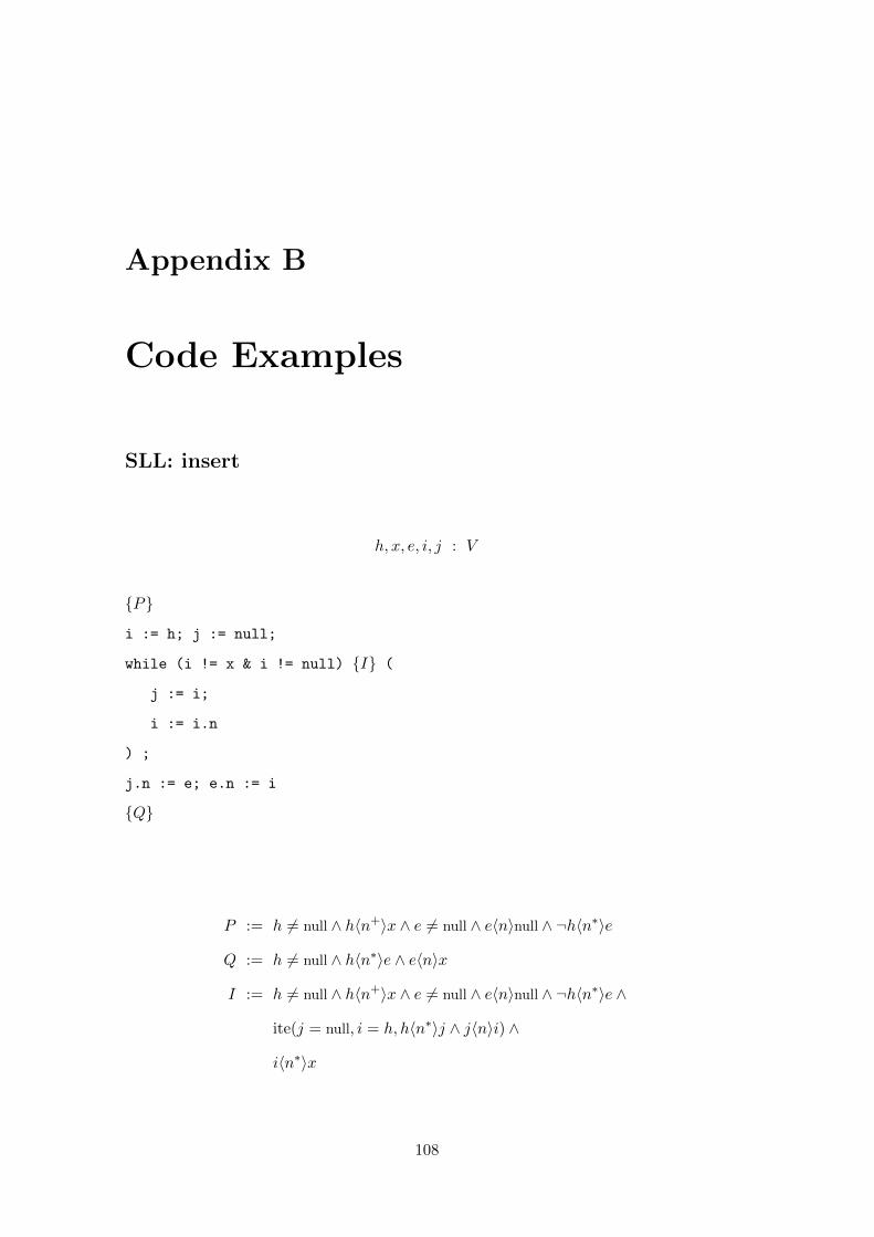
Appendix B
Code Examples
SLL: insert
h, x, e, i, j : V
{P}i := h; j := null;
while (i != x & i != null) {I} (
j := i;
i := i.n
) ;
j.n := e; e.n := i
{Q}
P := h 6= null ∧ h〈n+〉x ∧ e 6= null ∧ e〈n〉null ∧ ¬h〈n∗〉e
Q := h 6= null ∧ h〈n∗〉e ∧ e〈n〉x
I := h 6= null ∧ h〈n+〉x ∧ e 6= null ∧ e〈n〉null ∧ ¬h〈n∗〉e ∧
ite(j = null, i = h, h〈n∗〉j ∧ j〈n〉i) ∧
i〈n∗〉x
108

109
SLL: delete
h, i, j : V
C : V → {true, false}
{P}i := h ; j := null ; t := null ;
while (i != null & t = null) {I} (
if (C(i)) then t := i
else (
j := i ; i := i.n
)
) ;
if (i != null) then (
if (j = null) then h := i.n
else ( t := i.n ; j.n := null ; j.n := t )
)
else skip
{Q}
assumptions: ¬C(null), x, y 6= null
P := h〈n∗〉x ∧ x〈n∗〉y
Q := x〈n∗〉y ↔ (x = y ∨ y 6= i)
I := h〈n∗〉x ∧ x〈n∗〉y ∧
(i 6= null→ h〈n∗〉i) ∧
ite(j = null, i = h, h〈n∗〉j ∧ j〈n〉i) ∧
(∀m(h〈n∗〉m→ ¬i〈n∗〉m→ ¬C(m))) ∧
(t 6= null→ C(i))

110 APPENDIX B. CODE EXAMPLES
SLL: deleteAll
h, i, j : V
{P}i := h;
while $i != null$ $I$ (
j := i ;
i := i.n ;
j.n := null
)
{Q}
P := ∀xy(x〈n∗〉y ↔ x〈n∗〉y)
Q := ∀x(h〈n∗〉x→ x〈n〉null)
I := ∀mw(i〈n∗〉m→ (m〈n∗〉w ↔ m〈n∗〉w)) ∧
∀m(h〈n∗〉m ∧ ¬i〈n∗〉m→ m〈n〉null) ∧
(i 6= null→ h〈n∗〉i)
SLL: filter
{P}i := h ;
j := null ;
while (i != null) {I} (
if (C(i)) then ( t := i.n ; j.n := null ; j.n := t ) else j := i ;
i := i.n
)
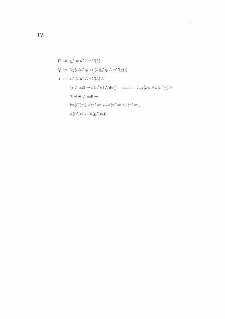
111
{Q}
P := n∗ = n∗ ∧ ¬C(h)
Q := ∀y(h〈n∗〉y ↔ (h〈n∗〉y ∧ ¬C(y)))
I := n∗ ⊆ n∗ ∧ ¬C(h) ∧
(i 6= null→ h〈n∗〉i) ∧ ite(j = null, i = h, j〈n〉i ∧ h〈n∗〉j) ∧
∀m(m 6= null→
ite(C(m), h〈n∗〉m↔ h〈n∗〉m ∧ i〈n∗〉m,
h〈n∗〉m↔ h〈n∗〉m))

Bibliography
[1] Mohamed Faouzi Atig, Ahmed Bouajjani, and Shaz Qadeer. Context-bounded
analysis for concurrent programs with dynamic creation of threads. Logical Meth-
ods in Computer Science, 7(4), 2011. 89
[2] Arnon Avron. Transitive closure and the mechanization of mathematics. In
FairouzD. Kamareddine, editor, Thirty Five Years of Automating Mathemat-
ics, volume 28 of Applied Logic Series, pages 149–171. Springer Netherlands,
2003. ISBN 978-90-481-6440-0. doi: 10.1007/978-94-017-0253-9 7. URL http:
//dx.doi.org/10.1007/978-94-017-0253-9_7. 28
[3] T. Ball, A. Podelski, and S.K. Rajamani. Boolean and Cartesian abstraction for
model checking C programs. 2001. 46
[4] Mike Barnett, Manuel Fahndrich, K. Rustan M. Leino, Peter Muller, Wolfram
Schulte, and Herman Venter. Specification and verification: the spec# experience.
Commun. ACM, 54(6):81–91, 2011. 66, 88
[5] Clark Barrett, Aaron Stump, , and Cesare Tinelli. SMTLIB: Satisfiability modulo
theories library, 2013. http://smtlib.cs.uiowa.edu/docs.html. 38, 86
[6] J. Berdine, C. Calcagno, B. Cook, D. Distefano, P.W. O’Hearn, T. Wies, and
H. Yang. Shape analysis for composite data structures. 2007. 47, 63
[7] Ahmed Bouajjani, Cezara Dragoi, Constantin Enea, and Mihaela Sighireanu. Ac-
curate invariant checking for programs manipulating lists and arrays with infinite
data. In ATVA, pages 167–182, 2012. 43
[8] A.R. Bradley. SAT-based model checking without unrolling. 2011. 45, 46, 48, 49,
53, 63
112

BIBLIOGRAPHY 113
[9] A. Cimatti and A. Griggio. Software model checking via IC3. 2012. 63
[10] P. Cousot and R. Cousot. Abstract interpretation: A unified lattice model for
static analysis of programs by construction or approximation of fixpoints. pages
238–252, 1977. 1
[11] L. de Moura and N. Bjørner. Z3: An efficient SMT solver. 2008. 47, 59
[12] L. De Moura and N. Bjørner. Z3: An efficient SMT solver. In TACAS, pages
337–340. Springer, 2008. 22
[13] Camil Demetrescu and Giuseppe F. Italiano. Decremental all-pairs shortest paths.
Encyclopedia of Algorithms, 2008. 5
[14] D. Distefano, P.W. O’Hearn, and H. Yang. A local shape analysis based on sepa-
ration logic. 2006. 47, 63
[15] N. Een, A. Mishchenko, and R.K. Brayton. Efficient implementation of property
directed reachability. 2011. 49, 63
[16] C. Flanagan and K. Rustan M. Leino. Houdini, an annotation assistant for Esc/-
Java. 2001. 62
[17] C. Flanagan and S. Qadeer. Predicate abstraction for software verification. 2002.
48, 54
[18] Cormac Flanagan and James B. Saxe. Avoiding exponential explosion: generating
compact verification conditions. In POPL, pages 193–205, 2001. 17, 37
[19] R. W. Floyd. Assigning meanings to programs. Mathematical aspects of computer
science, 19(19-32):1, 1967. 1, 12
[20] M.J. Frade and J.S. Pinto. Verification conditions for source-level imperative pro-
grams. Computer Science Review, 5(3):252–277, 2011. 17
[21] P. Garg, C. Loding, P. Madhusudan, and D. Neider. Learning universally quanti-
fied invariants of linear data structures. 2013. 63
[22] P. Garg, P. Madhusudan, and G. Parlato. Quantified data automata on skinny
trees: An abstract domain for lists. 2013. 47, 63

114 BIBLIOGRAPHY
[23] Yeting Ge and Leonardo de Moura. Complete instantiation for quantified formulas
in satisfiabiliby modulo theories. In Proceedings of the 21st International Confer-
ence on Computer Aided Verification, CAV ’09, pages 306–320, Berlin, Heidelberg,
2009. Springer-Verlag. ISBN 978-3-642-02657-7. doi: 10.1007/978-3-642-02658-4
25. URL http://dx.doi.org/10.1007/978-3-642-02658-4_25. 23
[24] Alexey Gotsman, Josh Berdine, and Byron Cook. Interprocedural shape analysis
with separated heap abstractions. In SAS, 2006. 89
[25] S. Graf and H. Saıdi. Construction of abstract state graphs with PVS. 1997. 46
[26] L. Hendren. Parallelizing Programs with Recursive Data Structures. PhD thesis,
Cornell Univ., Ithaca, NY, Jan 1990. 96, 97
[27] J.G. Henriksen, J. Jensen, M. Jørgensen, N. Klarlund, B. Paige, T. Rauhe, and
A. Sandholm. Mona: Monadic second-order logic in practice. 1995. 39
[28] W. Hesse. Dynamic computational complexity. PhD thesis, Dept. of Computer
Science, University of Massachusetts, Amherst, MA, 2003. 5, 34, 43, 92, 94, 101
[29] C. A. R. Hoare. An axiomatic basis for computer programming. Commun. ACM,
12(10):576–580, 1969. ISSN 0001-0782. doi: http://doi.acm.org/10.1145/363235.
363259. 1, 12
[30] K. Hoder and N. Bjørner. Generalized property directed reachability. 2012. 49, 63
[31] Krystof Hoder, Laura Kovacs, and Andrei Voronkov. Invariant generation in vam-
pire. In TACAS, pages 60–64, 2011. 62
[32] Neil Immerman. Descriptive Complexity. Springer-Verlag, New York, NY, USA,
1998. ISBN 0-387-98600-6. 33
[33] Neil Immerman, Alexander Moshe Rabinovich, Thomas W. Reps, Shmuel Sa-
giv, and Greta Yorsh. The boundary between decidability and undecidability
for transitive-closure logics. In CSL, pages 160–174, 2004. 28
[34] Neil Immerman, Alexander Moshe Rabinovich, Thomas W. Reps, Shmuel Sa-
giv, and Greta Yorsh. The boundary between decidability and undecidability
for transitive-closure logics. In CSL, pages 160–174, 2004. 6, 27

BIBLIOGRAPHY 115
[35] Samin S. Ishtiaq and Peter W. O’Hearn. Bi as an assertion language for mutable
data structures. In Proceedings of the 28th ACM SIGPLAN-SIGACT Symposium
on Principles of Programming Languages, POPL ’01, pages 14–26, New York,
NY, USA, 2001. ACM. ISBN 1-58113-336-7. doi: 10.1145/360204.375719. URL
http://doi.acm.org/10.1145/360204.375719. 2, 88
[36] Shachar Itzhaky, Anindya Banerjee, Neil Immerman, Aleksandar Nanevski, and
Mooly Sagiv. Effectively-propositional reasoning about reachability in linked data
structures. In CAV, volume 8044 of LNCS, pages 756–772, 2013. 6, 24
[37] Shachar Itzhaky, Anindya Banerjee, Neil Immerman, Ori Lahav, Aleksandar
Nanevski, and Mooly Sagiv. Modular reasoning about heap paths via effectively
propositional formulas. In The 41st Annual ACM SIGPLAN-SIGACT Sympo-
sium on Principles of Programming Languages, POPL ’14, San Diego, CA, USA,
January 20-21, 2014, pages 385–396, 2014. doi: 10.1145/2535838.2535854. 6, 65
[38] Shachar Itzhaky, Nikolaj Bjørner, Thomas W. Reps, Mooly Sagiv, and Aditya V.
Thakur. Property-directed shape analysis. In Computer Aided Verification - 26th
International Conference, CAV 2014, Held as Part of the Vienna Summer of Logic,
VSL 2014, Vienna, Austria, July 18-22, 2014. Proceedings, pages 35–51, 2014. doi:
10.1007/978-3-319-08867-9 3. 6, 44
[39] J. Jensen, M. Jorgensen, N. Klarlund, and M. Schwartzbach. Automatic verifi-
cation of pointer programs using monadic second-order logic. In Proceedings of
PLDI 97, 1997. 39
[40] Shuvendu K. Lahiri and Shaz Qadeer. Back to the future: revisiting precise pro-
gram verification using smt solvers. In POPL, 2008. 43, 92
[41] Gary T. Leavens, Albert L. Baker, and Clyde Ruby. Preliminary design of JML:
a behavioral interface specification language for java. ACM SIGSOFT Software
Engineering Notes, 31(3):1–38, 2006. 66, 88
[42] T. Lev-Ami and M. Sagiv. TVLA: A system for implementing static analyses.
pages 280–301, 2000. 11, 47
[43] T. Lev-Ami, N. Immerman, and M. Sagiv. Abstraction for shape analysis with
fast and precise transformers. 2006. 63
116 BIBLIOGRAPHY
[44] Tal Lev-Ami, Neil Immerman, Thomas W. Reps, Mooly Sagiv, Siddharth Sri-
vastava, and Greta Yorsh. Simulating reachability using first-order logic with
applications to verification of linked data structures. Logical Methods in Computer
Science, 5(2), 2009. 28, 43
[45] P. Madhusudan and X. Qiu. Efficient decision procedures for heaps using
STRAND. 2011. 63
[46] P. Madhusudan, Gennaro Parlato, and Xiaokang Qiu. Decidable logics combining
heap structures and data. In POPL, pages 611–622, 2011. 43
[47] R. Manevich, E. Yahav, G. Ramalingam, and Mooly Sagiv. Predicate abstraction
and canonical abstraction for singly-linked lists. 2005. 63
[48] A. Møller and M.I. Schwartzbach. The pointer assertion logic engine. pages 221–
231, 2001. 43
[49] G. Nelson. Verifying reachability invariants of linked structures. In POPL, 1983.
43
[50] Peter W. O’Hearn, John C. Reynolds, and Hongseok Yang. Local reasoning about
programs that alter data structures. In CSL, pages 1–19, 2001. 2
[51] R. Piskac, L. de Moura, and N. Bjørner. Deciding effectively propositional logic
using DPLL and substitution sets. J. Autom. Reasoning, 44(4):401–424, 2010. 56
[52] A. Podelski and T. Wies. Counterexample-guided focus. 2010. 63
[53] T. Reps, M. Sagiv, and G. Yorsh. Symbolic implementation of the best transformer.
pages 252–266, 2004. 54
[54] Thomas W. Reps, Mooly Sagiv, and Alexey Loginov. Finite differencing of logical
formulas for static analysis. ACM Trans. Program. Lang. Syst., 32(6), 2010. 43
[55] J. Reynolds. Separation logic: a logic for shared mutable data structures. In
LICS’02, 2002. xii, 2, 3
[56] Noam Rinetzky, Jorg Bauer, Thomas W. Reps, Shmuel Sagiv, and Reinhard Wil-
helm. A semantics for procedure local heaps and its abstractions. In POPL, pages
296–309, 2005. 9, 32, 68, 89
BIBLIOGRAPHY 117
[57] Noam Rinetzky, Mooly Sagiv, and Eran Yahav. Interprocedural shape analysis for
cutpoint-free programs. In SAS, pages 284–302, 2005. 89
[58] Xavier Rival and Bor-Yuh Evan Chang. Calling context abstraction with shapes.
In POPL, pages 173–186, 2011. 89
[59] M. Sagiv, T. Reps, and R. Wilhelm. Parametric shape analysis via 3-valued logic.
ACM Transactions on Programming Languages and Systems, 24(3):217–298, 2002.
47, 63
[60] Sriram Sankaranarayanan, Henny B. Sipma, and Zohar Manna. Scalable analysis
of linear systems using mathematical programming. In VMCAI, pages 25–41, 2005.
62
[61] Saurabh Srivastava and Sumit Gulwani. Program verification using templates over
predicate abstraction. In PLDI, pages 223–234, 2009. 62
[62] Robert Endre Tarjan. Efficiency of a good but not linear set union algorithm.
Journal of the ACM, 22(2):215–225, 1975. 11, 67
[63] A. Thakur, M. Elder, and T. Reps. Bilateral algorithms for symbolic abstraction.
2012. 54
[64] A. Thakur, A. Lal, J. Lim, and T. Reps. PostHat and all that: Automating
abstract interpretation. 2013. 54, 62
[65] A. Thakur, A. Lal, J. Lim, and T. Reps. PostHat and all that: Attaining most-
precise inductive invariants. TR-1790, Comp. Sci. Dept., Univ. of Wisconsin,
Madison, WI, April 2013. 62
[66] J. Wing. The CMU larch project. ”http://www.cs.cmu.edu/afs/cs/project/larch/www/home.html”,
1995. 66, 88
[67] Glynn Winskel. The Formal Semantics of Programming Languages: An Introduc-
tion. MIT Press, Cambridge, MA, USA, 1993. ISBN 0-262-23169-7. ix, 13, 14,
15
[68] G. Yorsh, T. Reps, and M. Sagiv. Symbolically computing most-precise abstract
operations for shape analysis. 2004. 63

118 BIBLIOGRAPHY
[69] G. Yorsh, T. Ball, and M. Sagiv. Testing, abstraction, theorem proving: Better
together! 2006. 54
[70] Greta Yorsh, Alexander Moshe Rabinovich, Mooly Sagiv, Antoine Meyer, and
Ahmed Bouajjani. A logic of reachable patterns in linked data-structures. J. Log.
Algebr. Program., 73(1–2):111–142, 2007. 43
[71] Karen Zee, Viktor Kuncak, and Martin C. Rinard. Full functional verification of
linked data structures. In PLDI, pages 349–361, 2008. 66, 88

:םיאבה םירמאמב ומסרופ תואצותה
• S. Itzhaky, A. Banerjee, N. Immerman, A. Nanevski, and M. Sagiv.
“Effectively-Propositional Reasoning About Reachability in Linked Data
Structures” in Computer Aided Verification, 2013, St. Petersburg,
Russia, July 2013.
• S. Itzhaky, A. Banerjee, N. Immerman, O. Lahav, A. Nanevski, and M.
Sagiv. “Modular Reasoning about Heap Paths via Effectively
Propositional Formulas” in 41st ACM SIGPLAN–SIGACT Symposium on
Principles of Programming Languages, San Diego, California, January
2014.
• S. Itzhaky, N. Bjørner, T.Reps, M. Sagiv, and A. Thakur, “Property-
Directed Shape Analysis” in Computer Aided Verification 2014,
Vienna, Austria, July 2014.

ילכב שומיש .רתוי הליעי הנכות תסדנה תבוטל )code reuse( שדחמ שומישל ןתינ
יוצרו ,םינוש םירשקה רפסמב עצובמ תויהל לוכי דיחי דוק עטקש ךכל םרוג הז יתונכת
םירשקהה ןמ דחאו דחא לכב דוקה עטק לש ותונוכנ תא אדוול ךרוצ היהי אלש דאמ
אדוול היהי ןתינ אלו יליבלקס אל תויהל חותינל םורגי הז ןכש ,דרפנב עיפומ אוה םהבש
תא עיבהל תלוכיה אוה רגתאה .תורודצורפ לש בר רפסמ תוליכמה תוינכת וז הטישב
המרעה לע הרודצורפה תעצבמש ,טקפאה וא ,הלועפה תא תצמתיש ןפואב ןוכדעה
,שיגנ וניא רחאה קלחהו הרודצורפל םישיגנ המרעה ירבאמ קלח רשאכ ,והשלכ רשקהב
frame( תרגסמ תייעב לש הרקמכ תאז תוארל רשפא .תונתשהל לוכי וניא חרכהב ךכיפלו
problem(.
.)reachability logics( תוגישי תוקיגול םשה תחת תוקיגול תחפשמ תגצומ הזתב
תודוא יתטיש קסיה ךרוצל םיישומיש ואצמנש םייגול םיעטקמ לש תילמרופ הרדגה תנתינ
הלא תוקיגול לש הקיטנמסה ,תירקיע הטישכ .םיעיבצמ םע םינבמ תוללוכה תוינכת
םיעדויה םייטמוטוא החכוה ילכב שומיש רשפאל תנמ-לע ןושאר רדסמ הקיגולב תעמטומ
ןתוא לש העבהה תלוכי לע הלבגמ ,םנמא ,הווהמ הז שומיש .וז הפשב טלק לבקל
קפסל ךרוצה ינפ-לע םייטמוטוא םילכב שומישהמ םיעבונה תונורתיה םלוא ,תוקיגול
םיכפוה ,ןהילאמ-תונבומ תוארנש תונטק תוינכתב רבודמשכ וליפא ,ינדי ןפואב תוחכוה
.ןתינש תע לכב יאדכל םהב שומישה תא

תועיפומ האלול תורומשש איה ךכל תירקיעה הביסה .םירוסא םניה םיתמכ יפוליח לבא
תפש יכ שרדנ ךכיפל ;תומיאה יאנת תא םינוב רשאכ הרירג רשק לש םידדצה ינשב
השירד תמייק אל יפוסה תומיאה יאנת רובעש דועב ,הלילש תחת הרוגס היהת תוזרכהה
.וזכ
לש ןוכדע תויעבב שומיש הב השענ הנורחאלש ךכמ תעבונ תירואית תויכוביסל היינפה
ונאש תוינכתש המרעב תוגישיה ינוכדעל הביבח הליבקמ שי וז היעבל .םינותנ יסיסב
ןוכדעל תשמשמה החסונה תויכוביסש ,תוארהל ןתינ view-update תייעבב .םינחוב
רשאמ רתוי הכומנ איה םינותנה סיסבב םישחרתמה םייוניש ינפ-לע התליאש תואצות
ךרוצ שי תוגישיה בושיח ךרוצל ,ןכא .הלחתההמ התליאשה בושיחל תשמשמה החסונה
ןושאר רדסמ םיחנומב אטבל ןתינ ןוכדע תואחסונש דועב ,יביטיזנרט רוגס םע החסונב
ה בצמל ״הנשי״ה תוגישיה תמאתה לש תויכוביסהש הדבועה תא םילצנמ ונחנא .דבלב
שומישל המוד םיצמאמ ונאש ןורתפה .תוגישי בושיח לש תויכוביסהמ הכומנ ״שדח״
םילולסמ רשאכ ,view-update תויעב ןורתפ רובע םיפרג לע םיימניד םיימתירוגלאב
ונלש ןורתפהש אלא ;תשק לש הפסוה וא הקיחמ ידכ ךות םינתשמ םיתמצ ןיב םינווכמ
ינבמ םירצויה םיעיבצמ תועצמאב םינוכדעה תא תועצבמה בשחמ תוינכתב לופיטל ןווכמ
.םירשוקמ םינותנ
5
quantifier-free formulas without transitive closure. In our setting, we compute reach-
ability relations instead of queries. We exploit the fact that the logical complexity of
adapting the (old) reachability relation to the updated heap is lower than computing
the new reachability relation from scratch. The solution we employ is similar to the use
of dynamic graph algorithms for solving the view-update problem, where directed paths
between nodes are updated when edges are added/removed (e.g., see [12]), except that
our solution is geared towards verification of heap-manipulating programs with linked
data structures.
statedatabase-update //
query
✏✏
state
query
✏✏qstate
query-update // qstate
Figure 1.3: The view update problem, natu-
rally occurring in databases but also applies
to heap reachability.
Another aspect that complicates pro-
grammatic reasoning, especially with
complex states as is the case when
pointer-based data structures are present,
is procedures. Programs are usually fac-
tored into several sub-programs in the in-
terest of readability and code reuse. This
common idiom causes one code block to
be executed in di↵erent contexts, and it is highly desirable for reasons of scalability
not to have to verify it for each context separately. The challenge is to be able to
express the view-update that summarizes the e↵ect of a procedure call in an arbitrary
context, where some of the elements are not reachable by the procedure, and therefore
essentially remain unmodified. This may be seen as an instance of the frame problem.
The rest of this thesis introduces reachability logics, a formal definition of logical
fragments found useful for the systematic reasoning over programs containing pointer
structures. As a primary technique, the semantics of such logics are embedded in
first-order logic for the use of automated solvers. While a severe limitation on the
expressivity of the defined logic, automated proof techniques prove to be so e↵ective
compared to manual proofs, even for small, seemingly-obvious examples, that there is
much benefit to using them whenever possible.
םהבש הלא ןוגכ םיבכרומ םיבצמב רבודמשכ דחוימב ,יתונכת קסיה ךבסמה ףסונ ןפ
בשחמ תוינכת .תורודצורפ אוה ,םיעיבצמ םיליכמה םינותנ ינבמ םימייק רשאכ םילקתנ
היהיו רתוי אירק היהי דוקהש תנמ-לע תאזו ,תוינכת-תת רפסממ ללכ-ךרדב תובכרומ

,היתובחרהו )Hoare logic( רוה תקיגול לש םיחותיפה לע רקיעב ססבתנ וז הזתב
החכוה תכרעמ איה רוה תקיגול .״רוה-חסונ תומיא״ ללוכה םשב ללכ-ךרדב תונוכמה
רקיעב - )assertions( תוזרכהכ םינותנה ןהיטרפמו תוינכת תודוא םיקסיה תכירעל
תיגול הפשב םיעבומ - )post-condition( רתב-יאנתו )pre-condition( םדק-יאנת
תויביטרפמיא תונכת תופש רובע תומלש החכוה תוכרעמ תומייקש דועב .ונתריחבל
לושכמה איה החכוהה שופיח תייעב ,)הדובעל עקרב תגצומ וזכ תכרעמל תחא המגוד(
ןוכנ הז .ןהיתונוכת תחכוהלו תוינכת תומיאל תיטמוטוא תכרעמ שומימל ךרדב ירקיעה
רשאכ דחוימב - םוצע אוה תוחכוהה בחרמש ןוויכ ,רתויב תונטק תוינכת רובע םג
לש והשלכ רפסמ ץורל דוק עטקל םורגל היושע תינכתב האלול .תואלול הליכמ תינכתה
וניא התציר ךלהמב תלקתנ תינכתה םהבש םינושה םיבצמה רפסמש ךכ ,םימעפ
םיבצמ לש תוצובקב םיקסועה םינועיטש רמול ןתינ סג ןפואב .תינכתה לדוגב ינויצרופורפ
.הובג רדסמ קסיה תייעב םיביצמ
.הטישה סיסבב תואצמנ תויזכרמ תונחבא יתש
next עיבצמה תא עיבהל ןתינ ,תורשוקמ-ודו תורשוקמ תומישר תולהנמה תוינכתב )א(
רשפאמ הז .המישרה ירביא ןיב תוגישי סחי תורחא םילימב וא ,םילולסמ לש םיחנומב
:)descriptive complexity( תירואיתה תויכוביסה תרותמ תושדח תואצותב חונ שומיש
דבאמ וניאש ןפואב המרעב םיכרענה םייונישל םאתהב תוגישיה סחי תא קזחתל רשפא
אלל ןניה ןוכדעה ךרוצל תושרדנה תומויסקאה ,דועו תאז .קיודמ אוה ךכיפלו עדימ
.םיתמכ
הקיגולב תומיא יאנת רצייל ןתינ ,המרעה תא תוקרוסש תוינכתב לפטל תנמ-לע )ב(
םילכ תרזעב םתותימא תא אדוול היהי ןתינש ךכ φ*∃*∀ היהת םתרוצש ןושאר רדסמ
הפשב תוזרכה בותכל רתוי תנכתמל .)ךשמהב רבסויש יפכ - SAT( תוקיפס תקידבל
next לש יביטיזנרט רוגסב שמתשהל ןתינ הבש ,ןושאר רדסמ הקיגול לש רתוי תמצמוצמ

תפסוה זא ,לולסמ הזכ םייק םא ןכש ,הצירה לש בלש םושב i ל j ןיב next-לולסמ
.המרעב תויוסחייתה לגעמ תרצוי i→j תשקה 3
1i 2 3 4 5
1 2
j
3
i
4 5
1 2 3 4 5 j
(i)
(ii)
(iii)
Figure 1.2: The state of the memory during the execution of the list reversal program:(i) initial state; (ii) an intermediate state; (iii) final state.
by i and each node contains a field next holding a pointer to the next node (or null
to signify the last node). The program outputs a list of the same structure, only that
the elements occur in reversed order. The reversal is done in-place, so that the original
input list is overwritten by the output.
Reynolds identified an acute problem when reasoning with programs that traverse
such recursive data structures: the pointer i serving as the iterator is advanced at each
step, and the number of steps is not bounded. Therefore there is always a risk that a
value written on one iteration will be overwritten in subsequent iterations. In particular,
to make sure that the list remains acyclic in this example, one must obtains that there
is no next-path from j to i, otherwise the addition of the edge i! j introduces a cycle.
We approach this problem by a careful construction of appropriate loop invariants
for iterative programs, and comprehensive summaries for recursive programs. Observ-
ing a typical run of reverse (Fig. 1.2), an important property of it can be noticed: the
pointer variables i and j always point into the beginning of two disjoint list segments.
Either segment may be empty (as in (i) and (iii)), but the segments never share el-
ements. It turns out that this property is crucial to prove the correctness of the list
reversal program. Formulating this property in logic is more involved than the previ-
ous, simpler aliasing conditions. To address this issue, we define reachability logics and
support reasoning to check the validity of implications. In this approach, we would
write an invariant such as
8↵ : ihnext⇤i↵ ^ jhnext⇤i↵! ↵ = null
While Reynolds proposed that such an approach would never scale, we show that for
many naturally occurring instances the invariants are quite managable and automatic
תוינכת רובע תומיאתמ האלול תורומש לש תינדפק הינב ידי-לע וז היעבל םישגינ ונא
םא .תויביסרוקר תוינכת רובע תורודצורפ לש םיקיודמו םימלש םיטרפמו ,תויביטרטיא
i םינתשמה :הבושח הנוכתב ןיחבהל ןתינ ,reverse תינכתה לש תינייפוא הצירב ןנובתנ
םיעטקמהמ דחא לכ .םירז המישר יעטקמ ינש לש םתליחת לע תע לכב םיעיבצמ j ו
.םיפתושמ םירביא םהל ויהי אל םלועל ךא ))iii( ו (i) םיבצמב ומכ( קיר תויהל יושע
.המישר ךופיהל תינכתה לש תונוכנה תחכוה רובע תיחרכה איה וז הנוכתש רבתסמ
הפיפחה יאנת םע ,תומדוקה תואמגודב רשאמ רתוי בכרומ הקיגולב הנעטה חוסינ
reachability( תוגישי תוקיגול םירידגמ ונא הלאכ םיחוסינ רשפאל ידכ .םיטושפה
logics( תא בותכנ ,וז השיגב .תועיבנו תורירג לש תונוכנ תחכוהל קסיה תוטיש םיקפסמו
:ךכ האלולה תרומש
∀α : i⟨next∗⟩α ∧ j⟨next∗⟩α → α = null
רובעש םיארמ ונא ,תיליבלקס היהת אל םלועל וז ןיעמ השיגש סרג סדלוניירש דועב
תוטישו לופיטל טלחהב תונתינ תורומשה תויתואיצמ תוינכתב םישחרתמה םיבר םירקמ
ךומתל תנמ-לע .םיריבס ןורכז תושירדו הציר ןמזב תורשפאתמ תויטמוטוא קסיה
המגודב .ירלודומ קסיהל תוקיגול חתפל םיכישממ ונחנא תולדגו תוכלוהה תוינכתב
.3 קרפב טוריפב ןודנ סדלונייר לש תיפיצפסה
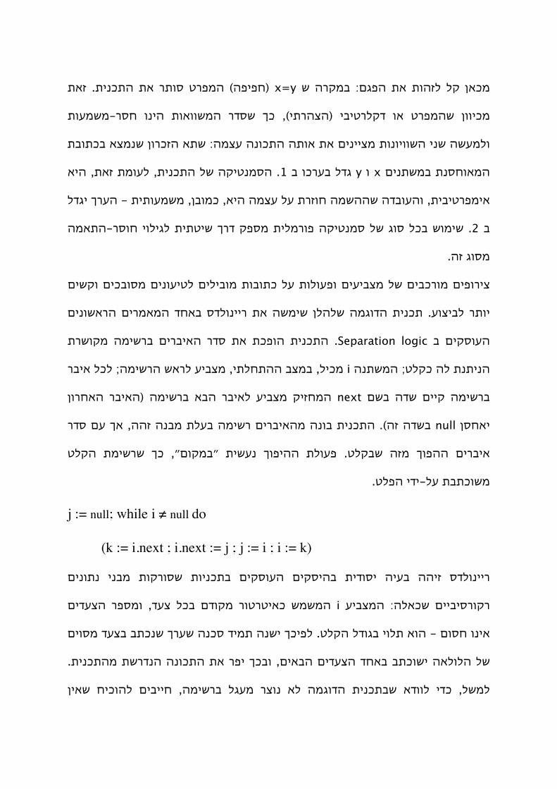
תאז .תינכתה תא רתוס טרפמה )הפיפח( x=y ש הרקמב :םגפה תא תוהזל לק ןאכמ
תועמשמ-רסח וניה תואוושמה רדסש ךכ ,)יתרהצה( יביטרלקד וא טרפמהש ןוויכמ
תבותכב אצמנש ןורכזה אתש :המצע הנוכתה התוא תא םינייצמ תונויוושה ינש השעמלו
איה ,תאז תמועל ,תינכתה לש הקיטנמסה .1 ב וכרעב לדג y ו x םינתשמב תנסחואמה
לדגי ךרעה - תיתועמשמ ,ןבומכ ,איה המצע לע תרזוח המשההש הדבועהו ,תיביטרפמיא
המאתה-רסוח יוליגל תיתטיש ךרד קפסמ תילמרופ הקיטנמס לש גוס לכב שומיש .2 ב
.הז גוסמ
םישקו םיכבוסמ םינועיטל םיליבומ תובותכ לע תולועפו םיעיבצמ לש םיבכרומ םיפוריצ
םינושארה םירמאמה דחאב סדלונייר תא השמיש ןלהלש המגודה תינכת .עוציבל רתוי
תרשוקמ המישרב םירביאה רדס תא תכפוה תינכתה .Separation logic ב םיקסועה
רביא לכל ;המישרה שארל עיבצמ ,יתלחתהה בצמב ,ליכמ i הנתשמה ;טלקכ הל תנתינה
ןורחאה רביאה( המישרב אבה רביאל עיבצמ קיזחמה next םשב הדש םייק המישרב
רדס םע ךא ,ההז הנבמ תלעב המישר םירביאהמ הנוב תינכתה .)הז הדשב null ןסחאי
טלקה תמישרש ךכ ,״םוקמב״ תישענ ךופיהה תלועפ .טלקבש הזמ ךופהה םירביא
.טלפה ידי-לע תבתכושמ
j := null; while i ≠ null do
(k := i.next ; i.next := j ; j := i ; i := k)
םינותנ ינבמ תוקרוסש תוינכתב םיקסועה םיקסיהב תידוסי היעב ההיז סדלונייר
םידעצה רפסמו ,דעצ לכב םדוקמ רוטרטיאכ שמשמה i עיבצמה :הלאכש םייביסרוקר
םיוסמ דעצב בתכנש ךרעש הנכס דימת הנשי ךכיפל .טלקה לדוגב יולת אוה - םוסח וניא
.תינכתהמ תשרדנה הנוכתה תא רפי ךכבו ,םיאבה םידעצה דחאב בתכושי האלולה לש
ןיאש חיכוהל םיבייח ,המישרב לגעמ רצונ אל המגודה תינכתבש אדוול ידכ ,לשמל

תולועפ עברא ומכ יסיסב הדובע יכ םה םיעיבצמ ,הרבצש הברה תוירלופופה בקע
םע הובג יוטיב רשוכ םיבלשמ םה .תינכתה לש הרקבה ינבמו הקיטמתיראב ןובשחה
הקיגול ,Seperation logic .תויביטימירפ ןורכיז תולועפ עוציבב הציר-ןמז תוליעי
לש ולא םירגתא לע תונעל דחוימב המאתוה ,ןרה׳ואו סדלונייר ידי-לע רקיעב החתופש
םע תוינכתב )aliasing( הפיפח לש תוחכונה בקע ,ללככ ,םילוע םירגתא .תונכתה
ןותנב יוניש ךכ-םושמו ,תבותכ התוא תא םיליכמ םיעיבצמ ינש ובש בצמ והז :םיעיבצמ
ןתינ .תינכתב תומוקמ ינשב תחא הנועבו תעב דימ ןימז ךפוה וז תבותכב ןסחואמה
:)C תפשב( האבה תינכתב ןויע ידי-לע תאז םיגדהל
void go_up(int *x, int *y) {
(*x)++; (*y)++;
}
הרקמב ,םלואו .y ו x ידי-לע םיעבצומה םינומה ינש תא םדקל התייה תנכתמה תנווכ
היהת האצותה ,)םיפפוח םה( תבותכ התואל עיבצמ םיליכמ y ו x םירטמרפה ובש הצק
לולע אוה ,הזכ שיחרתל ןנוכתה אל תנכתמה םא .2 ב דיחי הנומ לש הלדגה :היופצ אל
תונוכנ תא חיכוהל ןויסינ .רותיאל םישקו םינידע םיגאבלו הציר-ןמז תואיגשל ליבוהל
ידי-לע ןיפואמה הז לשמל ,הרובע ירשפא טרפמ חוסינל דימ איבי ילמרופ ןפואב הרגשה
:תואוושמה
[x] = [x] + 1
[y] = [y] + 1
x עיבמ ,ינסרה יוניש תועצבמה תוינכת לש םינויפאב לבוקמכ ,ןאכ עיפומה ןומיסב רשאכ
טלפה ךרע תא עיבמ x וליאו ,יונישה ינפלש בצמב ,x תינכתה הנתשמ לש טלקה ךרע תא
םינסחואמה םיכרעל תוסחייתה םינייצמ םיעבורמה םיירגוסה .יונישה ירחא ולש
.תונתשמ ןניאש ,ןמצע תובותכל םוקמב ,האוושמבש הנתשמה ידי לע תעבצומה תבותכב

ריצקת
תושועה בשחמ תוינכת תונוכנ לש תיטמוטוא החכוה ךרוצל םיעצמא הגיצמ וז הזת
ןוגכ ,םירשוקמ םינותנ ינבמ תולהנמש תוינכת תוללוכ הלא .םיעיבצמב בחרנ שומיש
ךרוצל .םיכפוהמ םיצעו תוננוקמ תומישר ,תורשוקמ-וד תומישר ,תורשוקמ תומישר
תיתשתה .לעופב החכוה םתוליעישו הישעתב טרדנטסל ויהש םילכב םישמתשמ ןוכימה
.תויגול תותליאש לש הרדסל תומיאה תייעב לש היצקודר לע תססובמ תעצומה תיגולה
וא ״ןכ״( תטלחומ הבושת ךכיפל ,העירכ הצובקב תוללכנו תיטמוטוא תורצוימ הלא
.הרקמ לכב תחטבומ )״אל״
דיולפ םירקוחה .המצע הנכותה לש המויק תליחת זאמ תמייק הנכותה תומיא תייעב
טרפמ לומ-לא בשחמ תוינכת לש תונוכנ תוחכוה תכירעל תיגול תיתשת ומזי רוהו
ןמז ךות תרצוע הנודנה תינכתהש החכוה תללוכ רשא ,האלמ תונוכנ תחכוה ןה ;ילמרופ
ןהו ,טרפמה תא תמאותה תוגהנתה םע דבב-דב ,הל תדעוימה טלקה תקלחמ לע יפוס
תוציר תרשפאמו השירדה תא הלקמ רשא ,תיקלח תונוכנ תחכוה לש רתוי ץופנה גוסה
םייקתהל ךישממ הלא תוחכוה תכירע ןוכימל ךשמתמ ץמאמ .תינכתה לש תורצוע אל
abstract( טשפומה שוריפה םוחת לש וחותיפל ואיבה וסוק גוזה .םויה דעו זאמ
interpretation(, תוינכות חותינ רובע רזע-תוטישו תוקינכט לש בחרנ ףסוא קפסמה
תודוה םיינרדומ םירדהמב ימוימוי שומישב תואצמנ הלא תוטיש .םינוש םיגוסמ
ןפואב .תוקפסמ ןהש םיבוטה םיעוציבהו ,שומימה תולק ,ןהלש תיטמתמה תויטנגלאל
המ ,תואצותה קויד ןיבל חותינל תשרדנה םיבאשמה תומכ ןיב חתמ דימת םייק ,יעבט
.תוברוקמ תואצות תוקפסמ םויכ שומישב תואצמנה תוזילנאה בורש ךכל ליבומש
תויעב לש הצובק דחוימב תניינעמ ,הנכות תומיאב תורושקה תויעבה בחרמ ךותמ
ורצונש היתורזגנבו C תפשב .םיעיבצמב בחרנ שומיש תושועה בשחמ תוינכתל תורושקה

הצובק לעמ תויביטקודניא תורומש לש תיטמוטוא הקסה רובע יביטרטיא ןודיע םתירוגלא
הנוב םתירוגלאה .םיבצמה בחרמ לש )היצקרטסבא( הטשפהל םישמשמה םיטקידרפ לש
דע םיגישיה םיבצמה תצובק תא הלעמלמ תומסוח רשא תוטשפה לש ףסוא הגרדהב
וז השיג .תשרדנה הנוכתה תא חיכוהל ליבשב קיפסמ הקזח הניהש הרומש תלבקתמש
רצייל חילצמ ונלש שומימהש וניארה .״property-directed reachability״ םשב העודי
.םימיאתמ םיטרפמ םע ןחוב-ירקמ לש הצובק רובע תונוכנ תורומש

תיצמת
גוסמ םינותנ ינבמ תולהנמה תוינכת לש תומיא תויעב רובע השדח הטיש תחסנמ וז הזת
השוע הטישה .םיכופה םיצע ומכ תוילוחב םישמתשמה םימוד םינבמו תרשוקמ המישר
תאז-םעו ,העירכ הניהש ןושאר רדסמ הקיגול לש תלבגומ הצובק-תתב שומיש
תימנידה המרעב תועבצה ירושיק לש םילולסמ תודוא קסיהב ךומתל ידכ היד תיביטקפא
,םינותנה הנבמ לש תוניקת ,הריצע חיכוהל ידכ תויחרכה הלאכ תונוכת .תינכתה לש
יביטיזנרט רוגס לש המלש תיטמויסקא הנרצה איה הזתה תביל .תופסונ תוחיטב תונוכתו
םותרל ןתינש ךכ ,)EPR( השעמל-תויקוספ תואחסונב ,ןושאר רדסמ הקיגולב יטסינימרטד
דגנ-תמגוד לש רוציי ךרוצל וא ,תופקת תחכוה ךרוצל SAT ןורתפל תומייק תוינכת
ולוכ לכומו תיגול םלש ןורתפהש ןוויכ .רפומ תומיאה יאנתש םירקמ רובע תיטרקנוק
םלועל הרגשה - תחטבומ הלא תואצותמ תחא ,ןושאר רדסמ הקיגול לש עירכ עטקמב
.תקיודמ-יתלב האצות הריזחמ הניאו תרדבתמ הניא
תמייק ,תורודצורפ תוליכמה תוינכתב .ירלודומ קסיהל תוקינכט ףסונב םיגיצמ ונא
היושע המרעה לש ןטק קלחב יוניש תעצבמש הרגש-תת :״ילבולג טקפא״ לש העפותה
ןוויכמ ,המרעב םינוש םימוקמב )העבצה ירושיק ךרד( תוגישי תונוכת לע עיפשהל
תולבגה ןנשי ךכיפל .םישדח םילולסמ תורצויו םימייק םילולסמ תוקתנמ הלש תולועפהש
שומיש השענ .עצבל תארקנה הרגשלו תארוקה הרגשל רוסא המו רתומ המ לע תומייוסמ
ךותב תארקנה הרגשה-תת התשעש םייונישה תא בלשל ידכ םיאתמ היצטפדא ללכב
.הל הארקש הרגשה לש המרעה בחרמ
רובע המיאתמ תיביטקודניא הרומש קפסל שרדנ שמתשמה ,וללה תוזילנאה יתשב
תויהל תולולעו ללכ תוילאיווירט ןניא תורומשה .תויביסרוקר תורודצורפ רובעו תואלול
ונמשיי ,וזה היעבה לע רבגתהל ידכ .הלוכ תינכתה לש טרפמה רשאמ רתוי תוכבוסמ


ש ריימונד ובברלי סאקלר"הפקולטה למדעים מדויקים ע ש בלבטניק"ס למדעי המחשב ע"ביה
היסק אוטומטי בתכניות עם מצביעים ידי לוגיקות כריעות-על
Ph.D– " דוקטור לפילוסופיה"חיבור זה הוגש כחלק מהדרישות לקבלת התואר
על ידי
שחר יצחקי
העבודה הוכנה בהדרכתו של
שגיב (מולי)שמואל ' פרופ
ד" תשעאלול


![Automated reasoning for equivalences in the …...Maude-NPA [23] and Tamarin [24] also use that notion, and Baudet [25] showed that diff-equivalence is decidable for a bounded num-](https://static.fdocuments.in/doc/165x107/5f2dc9e37c274957f425623b/automated-reasoning-for-equivalences-in-the-maude-npa-23-and-tamarin-24.jpg)