Automatic prediction of stock price direction

based on multivariate time series and machine

learning

Charlot Baldacchino

Faculty of ICT

Supervisor: Dr George Azzopardi

Co-supervisor: Mr Joseph Bonello

May 2016

Submitted in partial fulfilment of the requirements for the degree of

B.Sc. Artificial Intelligence (Hons.)

UNIVERSITY OF MALTA

FACULTY/INSTITUTE/CENTRE/SCHOOL__________________________

DECLARATION OF AUTHENTICITY FOR UNDERGRADUATE STUDENTS

Student’s I.D. /Code _____________________________

Student’s Name & Surname _________________________________________________

Course _________________________________________________________________

Title of Long Essay/Dissertation

________________________________________________________________________

________________________________________________________________________

________________________________________________________________________

I hereby declare that I am the legitimate author of this Long Essay/Dissertation and that it is my

original work.

No portion of this work has been submitted in support of an application for another degree or

qualification of this or any other university or institution of higher education.

I hold the University of Malta harmless against any third party claims with regard to copyright

violation, breach of confidentiality, defamation and any other third party right infringement.

______________________ ______________________

Signature of Student Date

11.06.2015

Abstract

The aim of this study is to predict the direction of the next closing price of Volk-

swagen AG. The study also concludes whether the stock price of Volkswagen, relies

on the prices of crude oil as well as EUR/USD exchange rate. Therefore, a mul-

tivariate time series is used to form feature vectors that consist of the historical

values of the same stock, prices of crude oil and prices of EUR/USD exchange rate.

The direction of the next closing price of Volkswagen is predicted by comparing

the performance of three supervised machine learning techniques namely, Support

Vector Machine (SVM), Artificial Neural Network (ANN) and Learning Vector

Quantization (LVQ). The study is focused on cross-validation of the three machine

learning techniques to get the best performance from each technique.

In the related works, a number of machine learning techniques are studied using

different stock markets. Therefore, to the best of my knowledge, the approach of

comparing SVM, ANN and LVQ for the prediction of the direction of a stock price

has never been investigated.

The system is designed to read three historical prices data and apply the data to

a Rate of Change indicator to standardize the prices. The data is used by the

three machine learning techniques to train a model and generate predicted labels

as output. The predicted labels are applied to a simple back testing strategy that

illustrate the profit or loss after five years. The predicted labels determine the

direction of the closing price of the next day. This is useful to calculate the hit rate

and performance of the techniques. Also, this will help investors decide whether to

buy, sell or hold to their investments.

The results conclude that ANN algorithm outperformed SVM and LVQ in regards

to the performance of the machine learning technique, as the former achieved the

highest hit rate of 52.24% during training of the model. The back testing results

show that SVM, leads to the highest profit when using the simple trading strategy

created.

iii

Acknowledgement

I would like to thank my principal supervisor Dr. George Azzopardi who over

the past year has provided me with valuable guidance and practical knowledge

throughout the dissertation.

I also would like to thank my co-supervisor Mr. Joseph Bonello for sharing his

expertise and giving me his feedback.

Finally, I would like to thank my family for their continuous support and encour-

agement.

iv

Contents

1 Introduction 1

1.1 Problem Definition . . . . . . . . . . . . . . . . . . . . . . . . . . . 1

1.2 Motivation . . . . . . . . . . . . . . . . . . . . . . . . . . . . . . . . 2

1.3 Approach . . . . . . . . . . . . . . . . . . . . . . . . . . . . . . . . 2

1.4 Scope . . . . . . . . . . . . . . . . . . . . . . . . . . . . . . . . . . 3

1.5 Aim and Objectives . . . . . . . . . . . . . . . . . . . . . . . . . . . 3

1.6 Report Layout . . . . . . . . . . . . . . . . . . . . . . . . . . . . . . 4

2 Background research and Literature review 5

2.1 Background research . . . . . . . . . . . . . . . . . . . . . . . . . . 5

2.1.1 Time Series . . . . . . . . . . . . . . . . . . . . . . . . . . . 5

2.2 Machine Learning . . . . . . . . . . . . . . . . . . . . . . . . . . . . 6

2.3 Literature review . . . . . . . . . . . . . . . . . . . . . . . . . . . . 7

3 Specification and Design 12

4 Implementation 16

4.1 Dataset . . . . . . . . . . . . . . . . . . . . . . . . . . . . . . . . . 16

4.2 Rate of Change . . . . . . . . . . . . . . . . . . . . . . . . . . . . . 17

4.3 Feature Extraction . . . . . . . . . . . . . . . . . . . . . . . . . . . 18

4.4 Supervised Machine Learning Algorithms . . . . . . . . . . . . . . . 19

4.4.1 Support Vector Machine . . . . . . . . . . . . . . . . . . . . 19

4.4.2 Artificial Neural Network . . . . . . . . . . . . . . . . . . . . 20

4.4.3 Learning Vector Quantization . . . . . . . . . . . . . . . . . 21

4.5 K-fold cross-validation . . . . . . . . . . . . . . . . . . . . . . . . . 22

4.6 Performance Measurements . . . . . . . . . . . . . . . . . . . . . . 23

4.7 Back Testing . . . . . . . . . . . . . . . . . . . . . . . . . . . . . . 24

5 Experiments and Results 25

6 Discussion 30

7 Future Work and Limitations 33

8 Conclusion 34

v

List of Figures

1 Time series data of Volkswagen AG closing stock price. . . . . . . . 5

2 The four stages of the system design of the proposed methodology . 12

3 The 5-fold cross-validation based model . . . . . . . . . . . . . . . . 14

4 The closing prices of the three datasets . . . . . . . . . . . . . . . . 16

5 The rate of change of the closing price of the three datasets . . . . . 17

6 The optimal hyperplane of SVM classification. . . . . . . . . . . . . 19

7 The diagram shows the three stages of Artificial Neural Network . . 21

8 The diagram shows the input data and the prototypes of the LVQ . 21

9 Schematic representation of a 5-fold cross-validation based model. . 22

List of Tables

1 The generated data labels by stock data . . . . . . . . . . . . . . . 13

2 The rules applied to the trading strategy to buy and sell stocks . . 15

3 Data Labels generated by Volkswagen AG closing stock price . . . . 18

4 The best performing parameter sets achieved from the cross-validation 25

5 The best results achieved on testing data . . . . . . . . . . . . . . . 28

vi

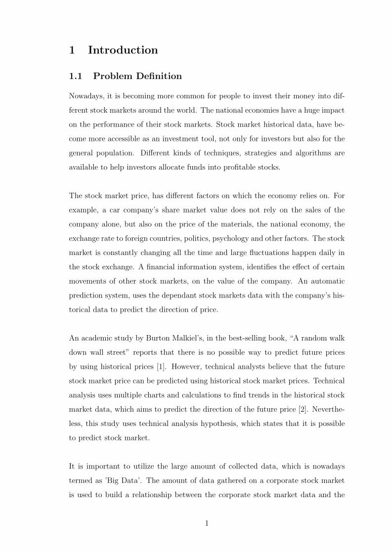
1 Introduction

1.1 Problem Definition

Nowadays, it is becoming more common for people to invest their money into dif-

ferent stock markets around the world. The national economies have a huge impact

on the performance of their stock markets. Stock market historical data, have be-

come more accessible as an investment tool, not only for investors but also for the

general population. Different kinds of techniques, strategies and algorithms are

available to help investors allocate funds into profitable stocks.

The stock market price, has different factors on which the economy relies on. For

example, a car company’s share market value does not rely on the sales of the

company alone, but also on the price of the materials, the national economy, the

exchange rate to foreign countries, politics, psychology and other factors. The stock

market is constantly changing all the time and large fluctuations happen daily in

the stock exchange. A financial information system, identifies the effect of certain

movements of other stock markets, on the value of the company. An automatic

prediction system, uses the dependant stock markets data with the company’s his-

torical data to predict the direction of price.

An academic study by Burton Malkiel’s, in the best-selling book, “A random walk

down wall street” reports that there is no possible way to predict future prices

by using historical prices [1]. However, technical analysts believe that the future

stock market price can be predicted using historical stock market prices. Technical

analysis uses multiple charts and calculations to find trends in the historical stock

market data, which aims to predict the direction of the future price [2]. Neverthe-

less, this study uses technical analysis hypothesis, which states that it is possible

to predict stock market.

It is important to utilize the large amount of collected data, which is nowadays

termed as ’Big Data’. The amount of data gathered on a corporate stock market

is used to build a relationship between the corporate stock market data and the

1

dependant fields in other stock markets or stock exchanges. Data should be filtered

to remove any information which has no impact on stock market prediction. Un-

derstanding the data collected is a huge factor in order to improve the predictive

powers of the model. The data gathered along the years can be used to config-

ure a model to predict the direction of a share in the following day/s. One idea

that emerges from the data collected is to predict the stock market based on what

people searched for the most or on their interest in these last few years.

1.2 Motivation

The prediction of stocks assist traders to predict the upcoming stock price direction

of a company. Thus, the investors would know when to buy undervalued stocks

and sell overvalued stocks. Stock prices are considered to change quite frequently

due to the financial domain and the factors affecting the company [3]. A skilled

and experienced trader, is more likely to guess to some extent the stock market

direction and to know when to buy and sell. Hence, if an algorithm can gain the

same experience from past data to improve the prediction for the future, it can

result into higher profits and fewer losses.

1.3 Approach

For this study, the approach taken is to compare three machine learning techniques,

namely Support Vector Machines (SVMs), Artificial Neural Networks (ANNs), and

Learning Vector Quantization (LVQ) for predicting the direction of Volkswagen

AG stock market. These supervised machine learning algorithms will be used to

configure classification models. Moreover, two other historical data, namely Crude

oil stock market and EUR/USD exchange rate are used for training the algorithms.

Using the three machine learning algorithms with the combination of the three

historical prices, it is possible to conclude which algorithm is the most effective to

predict the direction of the stock market. Nonetheless, there are various indicators

which may be used to support the algorithms to predict accurately, for instance,

the rate of change.

2

The classification models are trained using the first five years of the historical

closing price values. Afterwards, the model is used to predict the next day closing

price direction whether it is higher, lower or the same as the previous day. The

predicted labels are used into a simple back testing strategy that illustrates the

profit or loses using the last five years of historical data. The goal is to get the

highest profit using one of the machine learning techniques.

1.4 Scope

The scope of this study is to build a financial prediction system which will be able

to take a company’s last ten years of market share value to evaluate multiple time

series models to compare the historical prices of Volkswagen AG, prices of crude

oil and EUR/USD exchange rate. Along with Volkswagen stock market, two addi-

tional historical data prices are used to determine any dependency fields between

the three historical data prices which are expected to improve the performance.

The proposed work treats this challenge as a classification problem rather than

a regression problem. This means that the actual value of the stock will not be

predicted, but rather the direction of the closing prices, whether the price is higher,

lower or the same as the previous day.

After predicting the direction of the share market, the performance of each algo-

rithm is evaluated to see which algorithm is the most accurate to be used to invest

money and return profit. The back testing approach is used to accept the predicted

labels generated and apply the labels to the simple trading strategy created. The

result concludes if the machine learning used has led to profits or losses.

1.5 Aim and Objectives

The aim of this study is to use Volkswagen AG along with crude oil and exchange

rate to investigate the three techniques, namely SVM, ANN and LVQ to compare

the performance of the prediction. Using the data collected during the past five

years of the company, the aim is to predict whether the stock market direction

for the following day will be higher, lower or the same than the previous day.

3

Therefore, an accurate prediction of the direction of the closing price will help the

investors in investing money. In our case, we assume that the highest prediction

rate achieved from the three machines learning techniques along with a professional

trading strategy, will generated profit after five years. The objectives for this

project are:

• Finding the right stock data which are dependant to the company’s market

value.

• Using the first 5 years of market value, crude oil and currency exchange

historical data to train the system and the remaining 5 years to evaluate the

system accuracy.

• Making a performance comparison between the SVM, ANN and LVQ machine

learning techniques.

• Using back testing to determine the profit or loss that the proposed algorithm

leads to.

1.6 Report Layout

The second chapter discusses background information gathered about similar work

done in the past years. This will be used to help investigate more about the

proposed work. Further information on the specification and design of the project

will be evaluated in chapter 3, where details of how the system will be working

are analyzed. Chapter 3 explains the implementation of the proposed system. In

chapter 4, the effectiveness of the system and the methods used will be evaluated.

Chapter 5 discusses the output results of the system and how the results can be

improved. Chapter 6 provides a summary on the important aspects of the system

and indicators used, along with ideas for future work. Finally in chapter 7 the

conclusions will be drawn.

4

2 Background research and Literature review

2.1 Background research

Below are two definitions of the terms time series and machine learning.

2.1.1 Time Series

A time series [4] is a set of statistics which are collected at specific time intervals.

Figure 1 below, shows the time series of Volkswagen AG closing stock price for the

last 10 years. Time series is used in various sectors nowadays such as economics,

finance, environment and health. Automatic techniques use time series analysis for

different purposes, including clustering, classification query by content, anomaly

detection as well as forecasting. One method to describe time series is classical

decomposition which can be decomposed into four elements: trend, seasonal effects,

cycles and residuals. Trend is calculated by average, from long term movement

using symmetric moving average. If it is a seasonal effect, it can be estimated

using centered-moving average. Moving average is a calculation used to analyze

data points, by introducing a series of averages from different parts of the complete

data. A moving average applied repeatedly to a time series, can create artificial

cycles to smoothen the data [4].

Figure 1: Time series data of Volkswagen AG closing stock price.

5

2.2 Machine Learning

Machine Learning (ML) is the design of programs that can learn new rules from

training data, be able to adapt to changes, and improve system performance with

experience [5]. ML aims to understand the principles of learning as a computa-

tional process using several ways of categorization and characterization [6]. There

are various paradigms used in ML such as: generative, discriminative, supervised,

unsupervised, semi-supervised, active, adaptive, multi-task and Bayesian learning

paradigms. Below is a summary of two ML paradigms, which are mostly relevant

to this study.

Supervised learning requires that the data from which the model learns (training

data and training labels) is accompanied by the desired output. The output is

dependent on the user’s input parameters as learning rate and momentum con-

stant [7]. A supervised algorithm first learns a classification or a regression model

from the training data. A classification model learns a margin in the feature space

or in some other transformed space, whereas regression model learns a function.

The model trained is then used on test data or the so called unseen data. There

are various techniques of supervised learning algorithms such as: classification and

regression trees, k-Nearest Neighbour (KNN), Naive Bayes, SVM for classification

and regression, multi-class models for SVM, classification or regression ensembles

and tree ensembles, LVQ and ANN. Development of effective learning algorithms

gives some advantages since the problem of minimizing a function is well known in

other fields, such as in numerical analysis [8].

Unsupervised learning is used to identify patterns which are hidden in unlabelled

input data [9]. One type of unsupervised algorithms networks is the Self-Organizing

Feature Maps (SOM) which can also project high dimensional input space on a

low-dimensional topology, allowing one to visually determine the number of clusters

[10]. Among many clustering methods, the K-means method is the most frequently

used, since it is able to accommodate the large sample sizes associated with market

segmentation studies. Other types of unsupervised algorithms are the Gaussian

mixture model and hierarchical cluster analysis.

6

2.3 Literature review

Forecasting the short-term trend of a stock market is a very challenging task. The

parameters of stock markets, including opening price, closing prices, highest price,

lowest price and trading volume, were frequently used in previous studies to fore-

cast the stock market. The related work below believe the phenomenon that what

happened in the past can imply the occurrences of investment behaviour in the

future.

Two techniques, Support Vector Classification (SVC) and Support Vector Regres-

sion (SVR) were extended from support vector machine (SVM) to forecast the

movement direction of Google Inc. stock price [11]. Among four different time

periods tested, the moving trend within 30 days has achieved the highest accuracy

of 62.96% using SVC. Using SVR, the prediction accuracy data is obtained with

the same moving trend and the highest achieved result is 59.26%. Therefore, it was

concluded in [11] that using SVC to guide out investment in Google Inc. stock,

could get 63 times gains and 37 times losses from 100 trading lines. Another paper

used SVR technique with Takagi-Sugeno fuzzy rules-based model (TS model) to

identify daily stock trading from sets of technical indicators [12]. In the research,

the US stock market was used to compare the profit achieved. The main idea of

the paper was to find the fuzzy rule calculated by piecewise linear representation

(PLR) as PLR has 12 fuzzy rules to train the TS fuzzy model. Another study [12]

shows that the combination of SVR and TS fuzzy model is an excellent forecasting

tool to predict trading signals and identify trading thresholds.

Two studies [13] [14] shows that forecasting the movement direction can be im-

proved further with the best performing parameters for SVM. One research in-

vestigated the predictability of Least Square SVM (LSSVM) by predicting the

daily movement direction of China Security Index 300 (CSI 300) [13]. The results

show that LSSVM is superior to Probabilistic Neural Network (PNN) and to two

Discriminant analysis models (Quadratic Discriminant Analysis (QDA) and Lin-

ear Discriminant Analysis (LDA)). The other research [14] focused on Polynomial

Smooth SVM (PSSVM) to predict the movement of RMB (Chinese renminbi) vs

7

USD (United States Dollars) exchange rate with Dow Jones China Index Series.

Broyden-Fletcher-Goldfarb-Shanno (BFGS) method was used to solve PSSVM.

The research [14] says that the results achieved by PSSVM with a number of train-

ing data exceeding 118 trading days is 100%. In practice, the prediction can never

be 100% accurate as the exchange rate can vary with different factors such as wars,

earthquakes, influence diseases and political reasons among others [14].

Two studies [15] [16] agree that SVM with hybrid feature selection method is bet-

ter than SVM to predict the direction movement. One of the studies [15] uses

SVM with feature selection method based on fractal dimension and ant colony

optimization. The prediction model was used on the Shanghai Stock Exchange

Composite Index (SSECI) and 19 technical indicators. The results showed that

on average the improved fractal feature selection performed better than other fea-

ture selection methods when compared together. The other study [16] uses SVM

with F-score filter technique and supported sequential forward search. The paper

predicts the direction of the NASDAQ Index. The results showed that the pro-

posed model has the highest accuracies and better generalisation performance than

back-propagation neural network (BPNN). Another study proposed a hybrid ANN

model by combining the factor analysis for feature selection with feedback type of

functional link ANN (FFLANN) with Recursive Least Square (RLS) algorithm and

10 technical indicators [17]. The results shows that using Factor Analysis (FA) with

FFLANN-RLS provides the best performance for one and seven day/s prediction

for both DIJA and S&P 500 stock markets.

The use of technical indicators represent the features of generic price activity in

stock which effects the prediction results. A multilayer perceptron ANN archi-

tecture was used as a prediction model for Qatar Exchange (QE) with 10 market

technical indicators [18]. There are a mixture of reported results when comparing

ANN with ARIMA, however, this paper [18] proofs that ANN performed better

than ARIMA using QE stock market. The best performing ANN used was devel-

oped based on the ARIMA technique with a 3 year span as technical indicator.

Another paper uses ANN with 12 technical indicators to predict the movements of

8

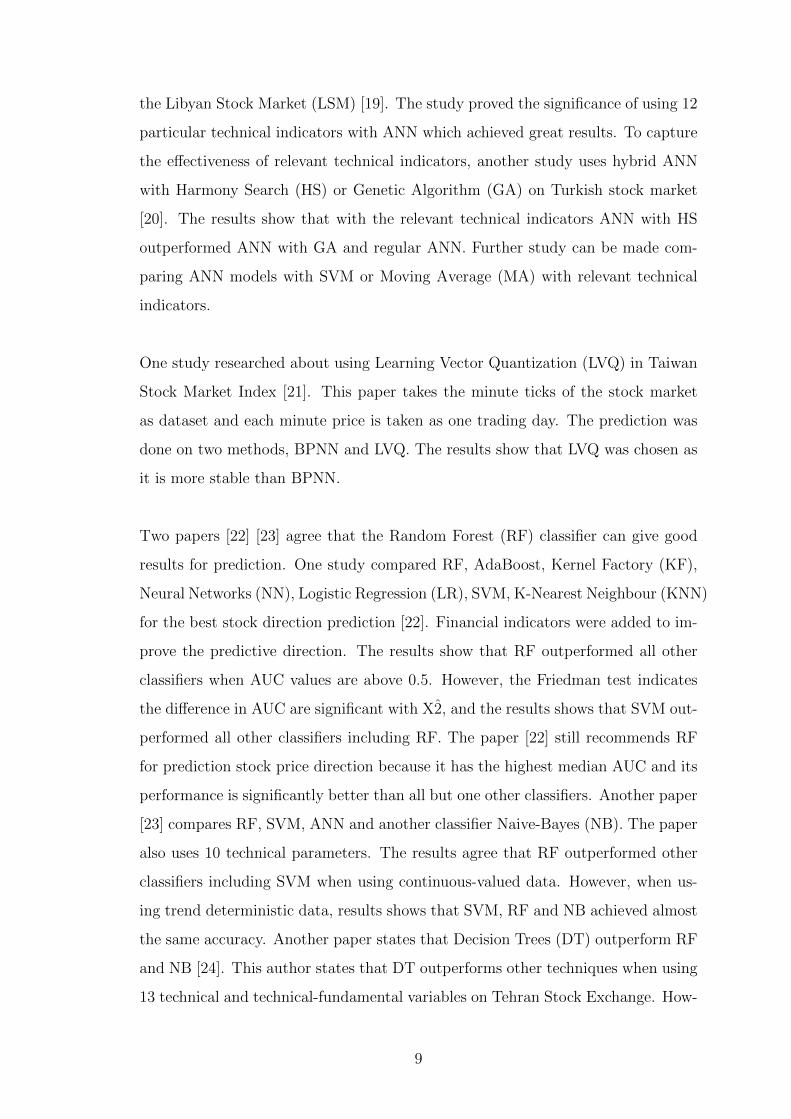
the Libyan Stock Market (LSM) [19]. The study proved the significance of using 12

particular technical indicators with ANN which achieved great results. To capture

the effectiveness of relevant technical indicators, another study uses hybrid ANN

with Harmony Search (HS) or Genetic Algorithm (GA) on Turkish stock market

[20]. The results show that with the relevant technical indicators ANN with HS

outperformed ANN with GA and regular ANN. Further study can be made com-

paring ANN models with SVM or Moving Average (MA) with relevant technical

indicators.

One study researched about using Learning Vector Quantization (LVQ) in Taiwan

Stock Market Index [21]. This paper takes the minute ticks of the stock market

as dataset and each minute price is taken as one trading day. The prediction was

done on two methods, BPNN and LVQ. The results show that LVQ was chosen as

it is more stable than BPNN.

Two papers [22] [23] agree that the Random Forest (RF) classifier can give good

results for prediction. One study compared RF, AdaBoost, Kernel Factory (KF),

Neural Networks (NN), Logistic Regression (LR), SVM, K-Nearest Neighbour (KNN)

for the best stock direction prediction [22]. Financial indicators were added to im-

prove the predictive direction. The results show that RF outperformed all other

classifiers when AUC values are above 0.5. However, the Friedman test indicates

the difference in AUC are significant with X2, and the results shows that SVM out-

performed all other classifiers including RF. The paper [22] still recommends RF

for prediction stock price direction because it has the highest median AUC and its

performance is significantly better than all but one other classifiers. Another paper

[23] compares RF, SVM, ANN and another classifier Naive-Bayes (NB). The paper

also uses 10 technical parameters. The results agree that RF outperformed other

classifiers including SVM when using continuous-valued data. However, when us-

ing trend deterministic data, results shows that SVM, RF and NB achieved almost

the same accuracy. Another paper states that Decision Trees (DT) outperform RF

and NB [24]. This author states that DT outperforms other techniques when using

13 technical and technical-fundamental variables on Tehran Stock Exchange. How-

9

ever, using fundamental indicators RF still outperforms DT and other techniques.

Another two papers [25] [26] which compared SVM and ANN, achieved different

results when classifiers were modified. One study used Korean and Hong Kong

stock markets with an integrated machine framework that employs Principal Com-

ponent Analysis (PCA) [25]. The results showed that the influence of PCA is

positive as both PCA-SVM and PCA-ANN outperformed the original SVM and

ANN. This author proposes PCA-SVM as it gave higher average hit ratios with

standard derivation. However, in another study, [26] the ANN model is compared

with polynomial SVM which is better than the standard SVM. Using ten indica-

tors on the Istanbul stock exchange, ANN performed significantly better than the

polynomial SVM.

Other papers proposed different ways to predict the direction of the stock mar-

ket. One study considered the predictive ability of the binary dependent dynamic

model in predicting the direction of monthly excess stock returns [27]. The pro-

posed forecast model using S&P500 stock performed better in the number of sign

predictions and investment returns compared with other models, ARMAX models

or predictive models. Another paper applied the prototype generation classifiers

to predict the trend of the NASDAQ Composite Index [28]. Prototype generation

classifiers are based on new artificial prototypes from training dataset to improve

the performance of the nearest neighbour. Four technical indicators [28] are used

from which the best result was provided by Modified Chang’s algorithm (MCA)

which outperformed standard Neural network and SVM.

One study [29] proposed Casual Feature Selection (CFS) to identify causalities

between variables based on the prediction model results [29]. Using the Shanghai

Stock exchange, CFS performed better than PCA, DT and the Least Absolute

Shrinkage and Selection Operator (LASSO). CFS performed best in terms of

accuracy, precision and considered the most stable compared to other algorithms.

CFS performed best when combined with SVM, J48 or RF in case of absolute

return and with SVM and RF in case of excess return. Two other studies analysed

10

stocks when methods such as Typical Price (TP), Bollinger Bands (BB), Relative

Strength Index (RSI), Chaikin Money Flow indicator (CMI) and Moving Average

(MA) are combined [30] [31]. Results by [30] concluded that the combination of

methods is able to perform better than random with some level of significance.

The more detailed results from [31] states that the combinational algorithm

Bollinger band crossover BSRCTB performed better than all the other methods

including Bollienger Signal (BS) and Stochastic Momentum Index (SMI).

Two other algorithms such as Multi Objective Particle Swarm Optimization

(MOPSO) and Nondominated Sorting Genetic Algorithm version-II (NSGA-II)

have been introduced to train the stock market prediction [32]. The experiments

were carried out using S&P 500, DIJA and Bombay stock exchange (BSE) stock

indices. Fuzzy logic based selection strategy was used to choose the best solution.

The results show that in terms of mean average percentage of error (MAPE) and

directional accuracy (DA), MOPSO and NSGA-II showed improved performance

compared to single objective based models like particle swarm optimization (PSO)

and genetic algorithm (GA). Furthermore the best performance was done by

MOPSO with PSO.

Above, a research of the tools, methods and approaches is conducted using different

studies which discuss the prediction of price, volume or direction of the stock

market value. In this work, the performance of three supervised machine learning

techniques are compared, namely SVM, ANN and LVQ, in combination with the

prices of crude oil, EUR/USD exchange rate and the closing prices of the stock

of Volkswagen AG. To the best of my knowledge, this approach has never been

investigated in previous studies.

11

3 Specification and Design

This study involves a financial information system which predicts the direction of

the stock price of the following day. The system is built using MATLAB. The

stock data prices required are downloaded from Google and Yahoo finance. The

datasets chosen for this study, namely Volkswagen AG stocks, crude oil stocks

and EUR/USD exchange rate, are applied to a Rate of Change (ROC) indicator

to standardize the prices. The system requires predicted labels to be used in the

trading strategy. The predicted labels are generated using three supervised machine

learning techniques, namely SVM, ANN and LVQ. Therefore, the system needs the

implementation of the three techniques with a cross-validation based model to

find the best set of parameters for each technique. The goal is to compare the

three techniques to conclude which algorithm is the most effective to predict data

labels, which leads to maximum hit rate accuracy. The system calculates the hit

rate accuracy of a machine learning technique by comparing the predicted labels

generated with the real labels in the test set. Finally, the system requires a back

testing strategy which uses predicted labels as input parameters, and with a trading

strategy, it is concluded whether the predicted labels actually resulted in a profit

or loss from the initial investment money.

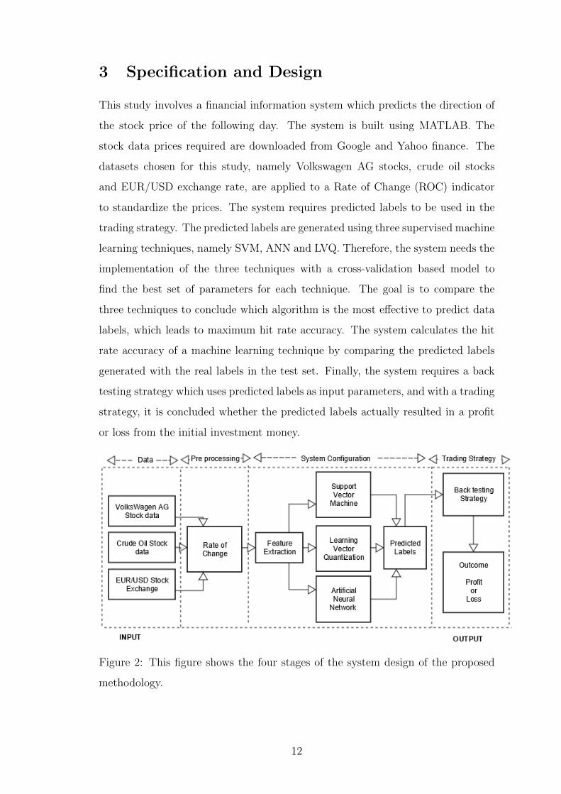
Figure 2: This figure shows the four stages of the system design of the proposed

methodology.

12

Figure 2 illustrates a system level block diagram which represents the four stages

of the system, namely: reading data, pre-processing data, training the machine

learning algorithm and back testing. The initial stage is reading the stock data

where the system takes as input from one to three stocks. This can be achieved by

either using the history of VW stock data alone, or else VW stock data and crude

oil data or VW stock data, crude oil and EUR/USD exchange rate. Volkswagen

stock data is always used throughout each training data.

The second stage is setting the data to be used by the machine learning techniques.

The stock data values are applied to an indicator called Rate Of Change (ROC).

ROC is the rate that describes how one quantity changes in relation to another

quantity. The ROC is important as it brings the three series within the same ranges,

and thus eliminates the risk of having the ones with high ranges dominating the

others.

Label VW Stock Data

1 stock data yesterday < stock data today

0 stock data yesterday = stock data today

-1 stock data yesterday > stock data today

Table 1: Data labels are generated by the stock data of the day before and the

current day.

The third stage involves three parts, namely: feature extraction, training the

machine learning techniques and the predicted labels. The feature extraction

involves data labels and data values. Data labels are generated using Volkswagen

closing stock data prices by the concept that if the price from one day to another

decreases, increases or remain the same, the label will be set to -1, 1 or 0

respectively, as shown in Table 1 above. Simultaneously, data values are created

according to the history span of each historical dataset prices. The data values

variable consists of the sum of the history span of the three datasets as columns,

and the number of trading days as rows. The history span is the number of days

used to represent the respective dataset in a single row.

13

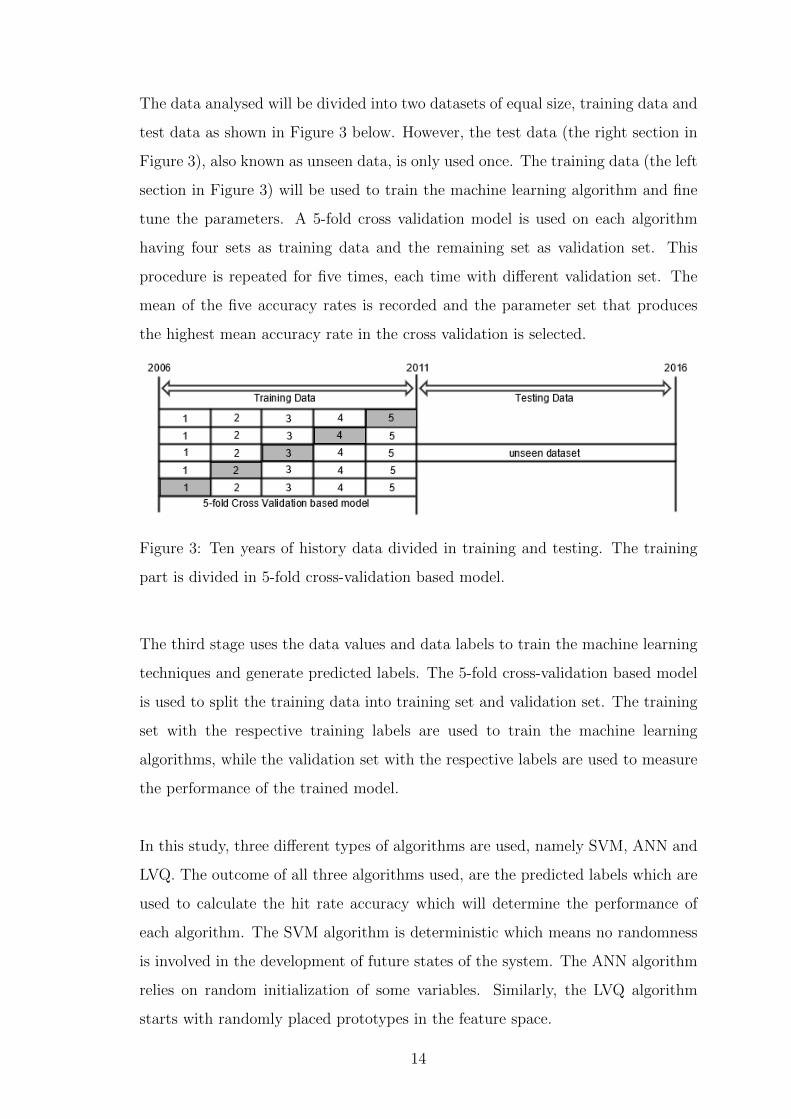
The data analysed will be divided into two datasets of equal size, training data and

test data as shown in Figure 3 below. However, the test data (the right section in

Figure 3), also known as unseen data, is only used once. The training data (the left

section in Figure 3) will be used to train the machine learning algorithm and fine

tune the parameters. A 5-fold cross validation model is used on each algorithm

having four sets as training data and the remaining set as validation set. This

procedure is repeated for five times, each time with different validation set. The

mean of the five accuracy rates is recorded and the parameter set that produces

the highest mean accuracy rate in the cross validation is selected.

Figure 3: Ten years of history data divided in training and testing. The training

part is divided in 5-fold cross-validation based model.

The third stage uses the data values and data labels to train the machine learning

techniques and generate predicted labels. The 5-fold cross-validation based model

is used to split the training data into training set and validation set. The training

set with the respective training labels are used to train the machine learning

algorithms, while the validation set with the respective labels are used to measure

the performance of the trained model.

In this study, three different types of algorithms are used, namely SVM, ANN and

LVQ. The outcome of all three algorithms used, are the predicted labels which are

used to calculate the hit rate accuracy which will determine the performance of

each algorithm. The SVM algorithm is deterministic which means no randomness

is involved in the development of future states of the system. The ANN algorithm

relies on random initialization of some variables. Similarly, the LVQ algorithm

starts with randomly placed prototypes in the feature space.

14

The fourth and final stage is about the predicted labels which are used into a

simple trading strategy. The back testing strategy uses the predicted labels with

the Volkswagen opening stock data prices and follow the trading strategy rules as

shown in Table 2 below. The rules state when to buy or sell stocks according to

the predicted labels. For instance, if the price decreases for two days, increases

for a day and prediction states that the price will increase in the upcoming day,

stocks are bought. On the other hand, if the price increases for two days, decreases

for a day and prediction states that the price will decrease in the upcoming day,

stock are sold. The stocks are bought or sold using Volkswagen opening stock data

prices. The final result is the final balance after the back testing trading strategy.

Label -3 days -2 days -1 days present day

Buy down down up predict up

Sell up up down predict down

Table 2: This table shows the rules applied to the trading strategy to buy and sell

stocks using Volkswagen opening stock data.

These four stages shown in Figure 2, are repeated for the combination of three com-

ponents for each machine learning algorithm. The performance of each algorithm

is investigated by firstly considering the history of the VW stock price, secondly, by

considering the history of both the VW stock price and history of Crude Oil, and

finally, by considering the history of the EUR/USD exchange rate with the other

two datasets. The system takes into consideration two sets of best performing pa-

rameter set for two cases: maximum profit from trading strategy and the maximum

hit rate. Each machine learning technique, produces six sets of best performing

parameters sets, consisting of two sets for each combination. Therefore, each ma-

chine learning technique returns the maximum hit rate achieved and maximum

final balance from the trading strategy while monitoring the input parameters of

each technique. The history span and the training data (if it is normalised or not)

are also monitored. The best performing parameter set is used only once on the

unseen data as test set. The result shows the hit rate reached and the final balance,

after the trading strategy. All results are monitored and discussed in Chapter 5.

15

4 Implementation

4.1 Dataset

For this study I collected three different stock market indexes. The datasets

chosen for this study are, an automobile manufacturer company Volkswagen AG,

the crude oil stock market and EUR/USD exchange rate. The datasets chosen for

this study was brought from Google and Yahoo finance and the graphs of each

time series is shown in Figure 4 below. All three stock market indexes have a

10 year history data starting from 26 January 2006 till 29 January 2016 which

amounts to 2516 trading days. In Figure 4 below, the three graphs represent the

closing prices of VW stock, crude oil and EUR/USD exchange rate. The prices

of each time series varies differently from each other, however, the same amount

and the same exact dates are used as trading days. The blue line on each graph

splits the time series in half, where the left side data is used for training and the

right side is used for test. The closing price of VW stock is used to train the

models along with the closing prices of crude oil and stock exchange. Also the

VW closing stock price was used to generate the direction label from one trading

day to another and for back testing while calculating final balance. During this

study, the VW opening stock price was used during back testing to buy and sell

stocks with the opening price of the next day.

Figure 4: Three graphs which show the closing prices of VW stock, Crude oil stock

and EUR/USD exchange rate.

16

4.2 Rate of Change

The Rate Of Change (ROC) indicator is used to normalize the difference in change

of price from one day to another. In Figure 4, one can notice that the prices of

each time series have different ranges. Therefore, ROC is used to standardize

the prices between each time series. ROC calculation compares the current stock

market price with the price of the day before. The ROC indicator is applied

to every dataset. Therefore, each dataset has a proportional difference in stock

market price from one trading day to another.

The ROC is defined as follows:

ROC =closetoday − closeyesterday

closeyesterday

Below in Figure 5 one can see the same stock markets shows in Figure 4, after

applying ROC to them. Using the equation shown above, the values of each

stock market vary between 1 and -1 as one can see in Figure 5. Normalization

with ROC is important to bring the three series within the same ranges, and

thus eliminating the risk of having the ones with high ranges dominating the others.

Figure 5: Three graphs which show the rate of change of the closing price of VW

stock, Crude oil stock and EUR/USD exchange rate.

17

4.3 Feature Extraction

In Machine Learning (ML), feature extraction is used to represent the input

data in terms of feature vectors. A supervised ML algorithm accepts training

data and training labels among other parameters. In this study, the data labels

are generated using Volkswagen AG closing stock price. If the closing price of

yesterday is greater, smaller or the same as the closing price of today, the data

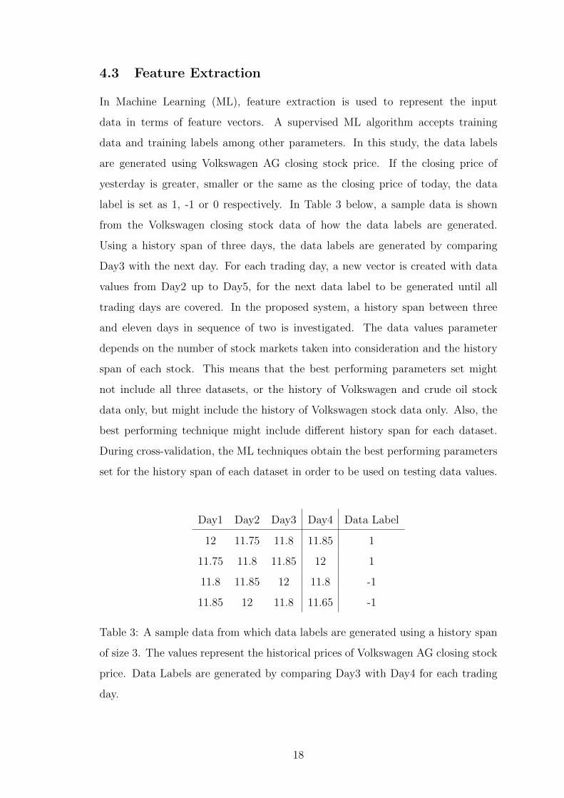
label is set as 1, -1 or 0 respectively. In Table 3 below, a sample data is shown

from the Volkswagen closing stock data of how the data labels are generated.

Using a history span of three days, the data labels are generated by comparing

Day3 with the next day. For each trading day, a new vector is created with data

values from Day2 up to Day5, for the next data label to be generated until all

trading days are covered. In the proposed system, a history span between three

and eleven days in sequence of two is investigated. The data values parameter

depends on the number of stock markets taken into consideration and the history

span of each stock. This means that the best performing parameters set might

not include all three datasets, or the history of Volkswagen and crude oil stock

data only, but might include the history of Volkswagen stock data only. Also, the

best performing technique might include different history span for each dataset.

During cross-validation, the ML techniques obtain the best performing parameters

set for the history span of each dataset in order to be used on testing data values.

Day1 Day2 Day3 Day4 Data Label

12 11.75 11.8 11.85 1

11.75 11.8 11.85 12 1

11.8 11.85 12 11.8 -1

11.85 12 11.8 11.65 -1

Table 3: A sample data from which data labels are generated using a history span

of size 3. The values represent the historical prices of Volkswagen AG closing stock

price. Data Labels are generated by comparing Day3 with Day4 for each trading

day.

18

4.4 Supervised Machine Learning Algorithms

4.4.1 Support Vector Machine

Support Vector Machine (SVM) is a training algorithm for learning classification

and regression rules from given data [33]. A kernel-based method, which can be

used with linear, polynomial, radial basis function (RBF) and other custom kernel

functions. SVM originated as an implementation of Vapnik’s (1995) Structural

Risk Minimization (SRM) principle to develop binary classifications [26]. Since in

this study three data labels are used and SVM is a binary classification tool, mean-

ing that it accepts only two classes at a time, an approach is adopted to deal with

the three classes. The SVM implementation used, is brought from the publicly

available LIBSVM, V3.17 [34]. The approach used is one-against-one classification

where SVM trains each class against another, having the most common prediction

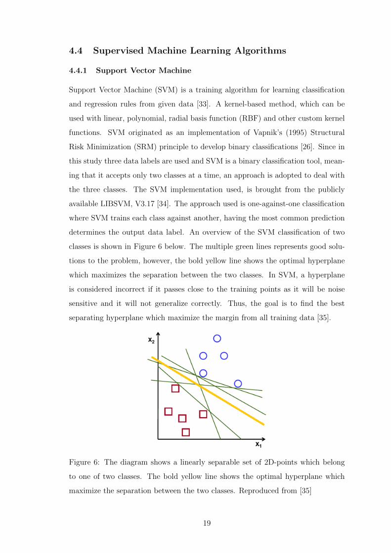
determines the output data label. An overview of the SVM classification of two

classes is shown in Figure 6 below. The multiple green lines represents good solu-

tions to the problem, however, the bold yellow line shows the optimal hyperplane

which maximizes the separation between the two classes. In SVM, a hyperplane

is considered incorrect if it passes close to the training points as it will be noise

sensitive and it will not generalize correctly. Thus, the goal is to find the best

separating hyperplane which maximize the margin from all training data [35].

Figure 6: The diagram shows a linearly separable set of 2D-points which belong

to one of two classes. The bold yellow line shows the optimal hyperplane which

maximize the separation between the two classes. Reproduced from [35]

19

The SVM classification model accepts training data, training labels and a variable

which contains information about how to train the SVM classifier to generate a

model. The choice of the SVM training data, kernel and kernel parameters are

automated by a cross-validation based model. In the cross-validation, the SVM

algorithm is trained with both L2-normalized data as well as not normalized data.

The SVM algorithm is trained with four types of kernel, namely: linear, polynomial,

radial basis and sigmoid kernel. Another parameter is the cost parameter, which

is investigated within a range of 10−6 to 103 in sequence of one.

4.4.2 Artificial Neural Network

The Artificial Neural Network (ANN), or simply neural network, is a machine

learning method evolved using the analogy of the human brain. ANNs make

predictions by sending the input data through the network of neurons, with the

neurons depending on the weights of the incoming signals. The final output is

determined by the strength of the signals coming from the hidden units as shown

in Figure 7 below.

MATLAB uses an inbuilt function named ’train’ to train the neural network. The

ANN first creates a pattern recognition neural network with selected number of

hidden layers chosen during cross-validation. The range of hidden layers that is

investigated ranges from one to eleven with a sequence of one. In the training

phase, the ANN uses a gradient descent algorithm to map input feature vector

with hidden units and hidden units with output unit. Using cross-validation, the

ANN algorithm is trained with both L2-normalized data as well as not normalized

data. The network is trained using training data and training labels parameters to

generate the output values. The output values are compared to a threshold value

determined by cross-validation which ranges from zero to 0.1 with an sequence of

0.02. If the output value of the newly trained model is greater, smaller, or within

the range of negative and positive threshold, stipulated by cross validation, then

the predicted label will be set to 1, -1 or 0 respectively. The predicted labels

are used to evaluate the hit rate accuracy of ANN and the final balance from the

trading strategy.

20

Figure 7: The diagram shows the three stages of Artificial Neural Network. The

input layer is as long as the length of the feature vector. Each element in the

feature vector is mapped to an input neuron. The feature vector consists of the

historical prices of each dataset according to each history span. For instance, a

VW stock history span of four days requires an input layer of four neurons. Each

neuron is mapped to a hidden unit. The output of each hidden unit depends on the

weights of the connections between the neurons and the hidden units. The hidden

layer is an encoding of which what the network considers to be the most significant

neurons. The output prediction depends on the the weights between the hidden

units and the output unit. Reproduced from [36]

4.4.3 Learning Vector Quantization

Another technique selected in this study is Learning Vector Quantization (LVQ).

LVQ is a supervised algorithm of Self-organising Maps (SOM) algorithm [38].

Figure 8: The diagram shows the input data and the prototypes of the Learning

Vector Quantization. Reproduced from [37]

21

LVQ uses prototype vectors to represent the labelled classes, as shown in Figure

8 above. The user can adjust the number of prototypes per class to be used. In

this study a total number of twenty-one prototypes are used for the three data

labels. LVQ randomly places prototypes in the feature space. The library provided

by Biehl [39] is used as a beginner tool for LVQ. Using cross-validation, the LVQ

algorithm is trained with both L2-normalized data as well as not normalized data.

The system performs various experiments where each time a different number of

prototypes per class is considered. The best number of prototypes per class is then

determined by cross validation on the validation set. The best prototype per class

is applied on the test set for the final prediction. The predicted labels of the LVQ

classification model as output are used to evaluate the hit rate accuracy of LVQ

and the final balance from the trading strategy.

4.5 K-fold cross-validation

The K-fold cross-validation based model is important for fine tuning the param-

eters of a prediction model. In this study, the proposed system uses a 5-fold

cross-validation. A cross-validation model allows you to find the best performing

parameters set for any machine learning technique without over fitting. In Figure

9 below, the training data is divided into five equal subsets in which one subset

represents the validation set and the other four subsets represent the training

Figure 9: Schematic representation of a 5-fold cross-validation based model. Re-

produced from [40]

22

data for the model. A five-fold cross-validation, iteratively repeats the process

for five times, each time using a different subset as validation set and the rest as

training data. After the iteration is completed, the hit rate of all five iterations

are considered and the average of the results is taken.

In this study, the results are the hit rate and the trading strategy outcome. If the

average maximum result is achieved in that particular test, the input parameters

for the machine learning technique are captured and stored for the best performing

parameters set.

Various cross-validation tests are performed in order to achieve the best performing

parameters using different variables. In general, the history span ranges from three

to eleven days in sequence of one each time while using a 5-fold cross validation. All

the best performing parameters of each machine learning technique for the average

hit rate and profit are used once on the testing data (unseen data).

4.6 Performance Measurements

The hit rate analyse the performance of each algorithm in percentage. The hit rate

of an algorithm shows the best performance of the algorithm with certain input

parameters set. The hit rate is determined using a confusion matrix including True

Positive (TP), True Negative (TN), False Positive (FP) and False Negative (FN).

The equation shown below shows how the hit rate is calculated.

Hit Rate =correct predicted labels

total number of testing labels× 100%

For instance if the prediction label is 1, and the actual label is 1, a true positive

is incremented as the prediction is correct. However, if for example the prediction

label is 0, and the actual label is -1, a false positive is incremented as prediction

is incorrect. The accuracy percentage of the hit rate is calculated by the sum of

all correct predicted labels divided by the sum of all testing labels. The higher the

accuracy hit rate reflects that the performance of one algorithm is better than the

other two algorithms to correctly predict the stock market direction.

23

4.7 Back Testing

Back testing is an evaluation technique that quantifies the performance of a

trading strategy in terms of profit and loss. A simple trading strategy is created

for the prediction of the proposed system. The currency chosen for this study

is euro since Volkswagen AG is a German car manufacturer which uses euro as

currency. The starting balance of the trading strategy is set to EUR10,000. The

amount of money used per trade is 10%, of the starting money. Therefore, if the

starting amount is EUR10,000, EUR1000 will be used per investment trade. There

is always a possibility to change the starting amount of money or the amount

of investment per trade. Also, a fee of EUR10 will be decreased from the cash

amount per buying or selling trade. Different investment services offer different

fees per trade, however, a simple strategy is used here. The strategy is built on

two basic factors which are the buy factor and the sell factor.

The strategy works by the theory of:

• Buy Factor : if the price during the previous three days, decreases in the

first and second day, but increases in the third day, and if the predicted

label states that the price will increase in the upcoming day, the system will

purchase 10% of the initial starting money.

• Sell Factor : if the price during the previous three days, increases in the first

and second day, but decreases in the third day, and if the predicted label

states that the price will decrease in the upcoming day, the system will sell

10% of the initial starting money.

The final balance will be accepted as the final outcome. The buying and selling

of stocks is done by the opening price of the following day. Moreover, after all

trading days are covered, the individual will sell all his stocks with the following

day opening price. The amount of money left will show if the prediction with the

strategy used actually generated money or not.

24

5 Experiments and Results

The proposed system compares three machine learning techniques, namely

SVM, ANN and LVQ. All three techniques are tested with the same data using

cross-validation based model. Each ML technique includes three tests having

different history stock prices as training data. Each technique uses a history span

from three to eleven days with a sequence of one each time. All tests are trained

with a 5-fold cross-validation based model. Each test has two best performing

parameters set: one for the average maximum hit rate and one for the average

maximum back testing return.

Table 4 below, shows a detailed description of the best performing parameters

set generated during the cross-validation on training data. The table shows all

three machine learning techniques, used with the best performing parameters set

including the specific historical datasets and the aim of the best parameter set

(average max final balance or average max hit rate). The information in Table 4,

is collected from the tests conducted on the first five years of historical data.

Table 4: The best performing parameter sets achieved from the cross-validation

model on training data.

25

The results from the SVM algorithm shows in Table 4, that the average maximum

final balance and hit rate are achieved using all three historical datasets. Out

of four types of kernels, the best performing parameters are generated using two

kernels. Out of six tests, four tests use sigmoid kernel and two tests use radial

basis kernel. The best performance parameters for SVM was conducted mostly

using L2-normalized data accept for one test.

The best performing parameter set for SVM in regards to the average maximum

hit rate was achieved with a hit rate of 50.72%. The history span for Volkswagen,

crude oil and EUR/USD exchange rate are three, nine, eleven respectively. The

training data used is L2-normalized with radial basis kernel and a cost parameter

of 1000. The best performing parameter set for SVM in regards to the average

maximum final balance was achieved with a final balance of EUR10,014.09.

The history span for Volkswagen, crude oil and EUR/USD exchange rate are

three, three, seven respectively. The training data used is L2-normalized with

sigmoid kernel and a cost parameter of 1000. It is noted that both best parame-

ters have the same Volkswagen history span and used L2-normalized data. The

cost parameter of both best parameters are 1000, however, a different kernel is used.

The results from the ANN algorithm shows in Table 4, that the average maximum

final balance and hit rate are achieved using all three historical datasets. Out of

six tests, the hidden layer varies between one to eleven hidden units. ANN on

Volkswagen stock data only uses a hidden layer of 11 hidden units on both best

parameters. Out of six parameters sets, the threshold varies between zero and

0.06. Three tests uses a threshold of zero for the best parameters set. Also, out of

six parameters sets, four tests use L2-normalised data.

The best performing parameter set for ANN in regards to the average maximum

hit rate was achieved with a hit rate of 52.24%. The history span for Volkswagen,

crude oil and EUR/USD exchange rate are three, three, eleven respectively.

The training data used non-normalized data, a threshold value of zero and size

of hidden layer set to one. The best performing parameter set for ANN in

26

regards to the average maximum final balance was achieved with a final balance

of EUR10,006.33. The history span for Volkswagen, crude oil and EUR/USD

exchange rate are seven, three, seven respectively. The training data used is

L2-normalized data, with a threshold of 0.02 and size of hidden layer set to three.

It is noted that both best parameters have the same crude oil history span. Also,

it is noted that the threshold for the best parameters to output predicted labels is

rather low.

The results from the LVQ algorithm shows in Table 4, that the average maximum

final balance and hit rate are achieved using all three historical datasets. Out of

six tests, three tests achieved the same number of prototype as the best parameter

set. Also, out of six parameters sets, five tests use L2-normalised data.

The best performing parameter set for LVQ in regards to the average maximum

hit rate was achieved with a hit rate of 50.88%. The history span for Volkswagen,

crude oil and EUR/USD exchange rate are three, five, seven respectively. The

training data used non-normalized data with a prototype of [1,2,3]. The best per-

forming parameter set for LVQ in regards to the average maximum final balance

was achieved with a final balance of EUR10,030.26. The history span for Volkswa-

gen, crude oil and EUR/USD exchange rate are eleven, eleven, eleven respectively.

The training data used is L2-normalized data with a prototype of [1,1,1,2,3]. It is

noted that both best parameters sets use L2-normalised data as training data.

27

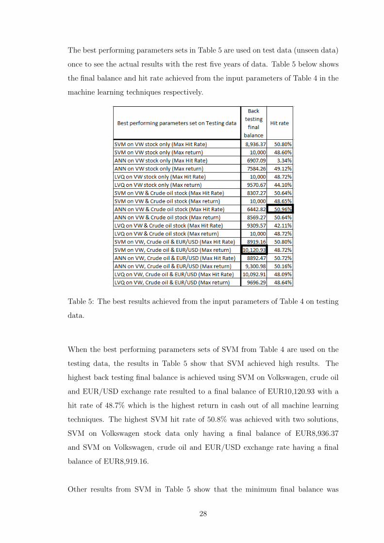
The best performing parameters sets in Table 5 are used on test data (unseen data)

once to see the actual results with the rest five years of data. Table 5 below shows

the final balance and hit rate achieved from the input parameters of Table 4 in the

machine learning techniques respectively.

Table 5: The best results achieved from the input parameters of Table 4 on testing

data.

When the best performing parameters sets of SVM from Table 4 are used on the

testing data, the results in Table 5 show that SVM achieved high results. The

highest back testing final balance is achieved using SVM on Volkswagen, crude oil

and EUR/USD exchange rate resulted to a final balance of EUR10,120.93 with a

hit rate of 48.7% which is the highest return in cash out of all machine learning

techniques. The highest SVM hit rate of 50.8% was achieved with two solutions,

SVM on Volkswagen stock data only having a final balance of EUR8,936.37

and SVM on Volkswagen, crude oil and EUR/USD exchange rate having a final

balance of EUR8,919.16.

Other results from SVM in Table 5 show that the minimum final balance was

28

EUR8,307.27 at a hit rate of 50.64% using SVM on Volkswagen and crude oil.

The minimum hit rate achieved was 48.6% at a final balance of EUR10,000 using

SVM on Volkswagen stock data only.

When the best performing parameters set of ANN from Table 4 are used on the

testing data, the results in Table 5 shows that ANN achieved high results too. The

highest back testing final balance is achieved using ANN on Volkswagen, crude oil

and EUR/USD exchange rate resulted to a final balance of EUR9,300.98 with a

hit rate of 50.16%. The highest ANN hit rate of 50.96% was achieved with ANN

on Volkswagen stock data crude oil only having a final balance of EUR6,442.82.

Also this is the highest hit rate achieved of all machine learning techniques.

However, the highest hit rate achieved by ANN of 50.96% resulted to the minimum

final balance of all techniques at EUR6,442.82. The minimum hit rate achieved

by ANN was 3.34% at a final balance of EUR6,907.09 using ANN on Volkswagen

stock data only.

When the best performing parameters set of LVQ from Table 4 are used on the

testing data, the results in Table 5 shows that LVQ achieved high results. The

highest back testing final balance is achieved using LVQ on Volkswagen, crude

oil and EUR/USD exchange rate resulted to a final balance of EUR10,092.91

with a hit rate of 48.09%. The highest LVQ hit rate of 48.72% was achieved

with two solutions, LVQ on Volkswagen stock data only having a final balance

of EUR10,000 and LVQ on Volkswagen and crude oil having a final balance of

EUR10,000 too.

Other results from LVQ in Table 5 shows that the minimum final balance was

EUR9,570.67 at a hit rate of 44.10% using LVQ on Volkswagen stock data only.

The minimum hit rate achieved was 42.11% at a final balance of EUR9,309.57 using

LVQ on Volkswagen and crude oil stock data.

29

6 Discussion

From the results stated in Table 4, the cross-validation done on training data

generated eighteen best performing parameters sets. Using SVM, the average

maximum final balance achieved during cross-validation is EUR10,014.09 with all

three historical prices. The average maximum hit rate using SVM achieved during

cross-validation is 50.72% with all three historical prices. In both cases (max final

balance and max hit rate) SVM was used and the best performing parameter set,

used all three historical prices with L2-normalised data and kernel cost value set

to 1000. It is noted that all SVM best performing parameters sets use sigmoid or

radial basis kernel. Therefore, polynomial and linear SVM kernels did not return

good results.

Using ANN, the average maximum final balance achieved during cross-validation

is EUR10,006.33 with all three time series histories. The maximum average hit

rate using ANN achieved during cross-validation is 52.24% with all three historical

prices. The ANN achieved the average maximum hit rate from all other techniques

during cross-validation. Nonetheless, the best ANN results use a threshold to

output predicted labels of 0 & 0.02 which is considered to be low. The hidden

layer size of the best ANN results are 1 & 3 which are rather low from a range of

11 hidden layer size.

Using LVQ, the average maximum final balance achieved during training is

EUR10,030.26 with all three historical prices. The LVQ achieved the maximum

final balance from all other techniques during cross-validation. The average

maximum hit rate using LVQ achieved during cross-validation is 50.88% with

all three historical prices. In both cases, maximum hit rate and maximum final

balance, LVQ achieved the best results using L2-normalised data and with all

three time series historical prices.

From the results stated in Table 5 above, all eighteen best performing parameters

sets are used on the rest of the 5 years as test data (unseen data). Using SVM,

the maximum final balance achieved using test data is EUR10,120.93 with a hit

30

rate of 48.72%. This result was achieved using the best performing parameters set

generated by SVM and all three historical prices while calculating maximum final

balance. Using SVM, the maximum hit rate achieved using test data is 50.8% with

a final balance of EUR8,919.36. This result was achieved by two best parameters,

SVM using Volkswagen stock data only and SVM with all three historical prices.

Using ANN, the maximum final balance achieved using test data is EUR9,300.98

with a hit rate of 50.16%. This result was achieved using the best performing

parameter set generated by ANN and all 3 time series histories while calculating

maximum final balance. Using ANN, the maximum hit rate achieved using test

data is 50.96% with a final balance of EUR6,442.82. This result was achieved

using the best performing parameter set, generated by ANN using VW & Crude

Oil stock data only, while calculating maximum hit rate. This result is the best

hit rate achieved using test data from the other techniques.

Using LVQ, the maximum final balance achieved using test data is EUR10,092.91

with a hit rate of 48.09%. This result was achieved using the best performing

parameter set generated by LVQ and all three historical prices while calculating

maximum hit rate. This result is the best final balance outcome achieved using

test data from the other techniques. Using LVQ, the maximum hit rate achieved

using test data is 48.72% with a final balance of EUR10,000. This result was

achieved twice using the best performing parameter set generated by LVQ. The

first time using only VW stock data while calculating maximum hit rate whereas

the second time using VW & crude oil stock data while calculating maximum final

balance.

The best performing parameters sets configured during cross-validation for

maximum final balance, show the highest result during the evaluation on the

testing data. However, the best performing parameters sets configured during

cross-validation for maximum hit rate, does not show the highest result during the

evaluation on the testing data on neither machine learning algorithm. The best

performing parameter set during configuration using SVM for maximum hit rate,

31

resulted to a maximum hit rate of 50.80% during evaluation on all three historical

prices, however, the same result was also achieved by SVM using only VW stock

data. Nonetheless, the highest hit rate of ANN and LVQ during configuration

was achieved using all three historical prices, whereas the highest hit rate during

evaluation was achieved using VW and crude oil stock data prices.

The results generated during the evaluation of the system on unseen data show

that whenever the hit rate exceeded the 50% hit rate, the back testing trading

strategy ended up with a loss. Taking into consideration the ANN algorithm, a

final balance of EUR6,907.09 was achieved with the minimum hit rate of 3.34%

whereas the highest hit rate obtained of 50.96% resulted into the greatest loss

with a final balance of EUR6,442.82. The highest hit rate achieved with a profit

final balance is 48.72% using SVM while the least hit rate achieved with a profit

final balance is 48.09%. This results that further improvement could been done on

the trading strategy.

From this study, one can agree with related work in the literature review where

ANN outperformed SVM in regards of performance. In fact ANN achieved a hit

rate of 50.96% and SVM achieved a hit rate of 50.8%. None of the studies researched

mention the comparison of LVQ with ANN nor SVM. This might result that LVQ

is the least performing machine learning compared with ANN and SVM. In fact the

best performance result using LVQ is 48.72%, which is 2% less than that achieved

by ANN and SVM.

32

7 Future Work and Limitations

During this present study, some limitations were found which held back the system

from further improvement. Some issues which were encountered were related to

the limitations of the processing speed of the hardware used. For instance, some

tests conducted using LVQ took over 34 hours of processing. Due to this factor,

other iterations were not added to the system for better cross-validation results.

Another limitation which affected the results is the trading strategy. A simple

trading strategy was created for the system to train and test the predicted labels,

however, some prediction generated did not allow transactions to take place during

back testing.

Improvements and changes are always important and necessary in this financial

sector. One important aspect for future work is an improved trading strategy with

cross-validation based model to achieve the best trading strategy for the predicted

labels. Due to the processing time of LVQ tests, several hours were taken and

additional improvements could not be added to the system which would have

affected the processing time to run the system. One improvement is including the

gross domestic product of the German economy which might be effective during

the training of the machine learning techniques.

Moreover, another improvement which could have been implemented is a cross-

validation based model on Volkswagen closing price data labels so that the best

threshold value on how data labels are chosen is selected. The threshold value

might affect the performance of the machine learning techniques because data labels

might have been chosen more equally. Further improvement could have been done

by increasing the range of history span used to train the models, preferably using

a sequence of one each time. Other indicators could have been considered which

might affected the performance of the machine learning techniques more than the

Rate of Change. Furthermore the cross-validation model on the size of training

data and testing data, could have been improved by cross-validate how the dataset

is divided. Lastly, each machine learning technique could have a wider range of

input parameter values. The SVM technique could have a wider range of C cost

33

parameter and another SVM type (nu-SVC) could have been tested additional to

the SVM types tested. The ANN technique could have a wider range of hidden layer

size and a wider range of threshold using a sequence of one. The LVQ technique

could have included more prototypes per class.

8 Conclusion

From this present study, the historical values of Volkswagen AG, crude oil

and EUR/USD exchange rate is a good combination for the machine learning

techniques. SVM and LVQ algorithms prove Volkswagen is dependent on crude oil

and EUR/USD exchange rate. However, the best machine learning technique for

stock price direction during this study was the ANN which achieved the highest

hit rate during configuration (52.24%) and evaluation (50.96%).

On training data, the highest hit rate is achieved with all three historical prices.

However, on testing data, the ANN achieved the highest hit rate using Volkswagen

and crude oil stock data only without EUR/USD exchange rate. Using ANN,

Volkswagen was more dependant on crude oil.

The performance of the three machine learning techniques was calculated by the

hit rate achieved. Therefore, one can conclude that ANN outperformed SVM and

LVQ in stock direction prediction. ANN predicted the most correct labels and is

considered superior over the other two techniques.

If we consider the results by applying the best performing parameters sets of

maximum hit rate for each machine learning technique configured during training

data, we end up having SVM with the maximum hit rate of 50.80%, Ann with a

hit rate of 50.72% and LVQ with the least hit rate of 48.09%. Therefore, using

the highest hit rate of each machine learning during evaluation result that SVM

achieved the highest rate during evaluation.

The predicted labels can be integrated in a more professional trading strategy in

order to help the investor making decisions.

34

References

[1] B.G. Malkiel. A Random Walk Down Wall Street: Including a Life-cycle

Guide to Personal Investing. Norton, 1999.

[2] InvestorGuide. Technical Analysis and How it is Used to Predict Stock

Prices. http://www.investorguide.com/article/11633/

technical-analysis-and-how-it-is-used-to-predict-stock-prices-igu/

?gcs=1.

[3] Salman Azhar, Greg J Badros, Arman Glodjo, Ming-Yang Kao, and John H

Reif. Data compression techniques for stock market prediction. In Data

Compression Conference, 1994. DCC’94. Proceedings, pages 72–82. IEEE,

1994.

[4] M. Phil. Time series. IEEE, 1999.

[5] Avrim Blum. Machine learning theory. In Department of Computer Science

Carnegie Mellon University. IEEE.

[6] Li Deng and Xiao Li. Machine learning paradigms for speech recognition: An

overview. Audio, Speech, and Language Processing, IEEE Transactions on,

21(5):1060–1089, 2013.

[7] Martin Fodslette Møller. A scaled conjugate gradient algorithm for fast

supervised learning. Neural networks, 6(4):525–533, 1993.

[8] R. L. Watrous. Learning algorithms for connectionist networks: Applied

gradient methods of nonlinear optimization. In International Conference on

Neural Networks, 2, 619-628. IEEE, 1987.

[9] R Sathya and Annamma Abraham. Comparison of supervised and

unsupervised learning algorithms for pattern classification. Int J Adv Res

Artificial Intell, 2(2):34–38, 2013.

[10] RJ Kuo, LM Ho, and Clark M Hu. Integration of self-organizing feature map

and k-means algorithm for market segmentation. Computers & Operations

Research, 29(11):1475–1493, 2002.

35

[11] Xuan Liu and Liu Pan. Prediction of the moving direction of google inc.

stock price using support vector classification and regression. Asian Journal

of Finance & Accounting, 6(1):323–336, 2014.

[12] Pei-Chann Chang, Jheng-Long Wu, and Jyun-Jie Lin. A takagi–sugeno fuzzy

model combined with a support vector regression for stock trading

forecasting. Applied Soft Computing, 38:831–842, 2016.

[13] Shuai Wang and Wei Shang. Forecasting direction of china security index

300 movement with least squares support vector machine. Procedia

Computer Science, 31:869–874, 2014.

[14] Yubo Yuan. Forecasting the movement direction of exchange rate with

polynomial smooth support vector machine. Mathematical and Computer

Modelling, 57(3):932–944, 2013.

[15] Li-Ping Ni, Zhi-Wei Ni, and Ya-Zhuo Gao. Stock trend prediction based on

fractal feature selection and support vector machine. Expert Systems with

Applications, 38(5):5569–5576, 2011.

[16] Ming-Chi Lee. Using support vector machine with a hybrid feature selection

method to the stock trend prediction. Expert Systems with Applications,

36(8):10896–10904, 2009.

[17] CM Anish and Babita Majhi. Hybrid nonlinear adaptive scheme for stock

market prediction using feedback flann and factor analysis. Journal of the

Korean Statistical Society, 2015.

[18] Adam Fadlalla and Farzaneh Amani. Predicting next trading day closing

price of qatar exchange index using technical indicators and artificial neural

networks. Intelligent Systems in Accounting, Finance and Management,

21(4):209–223, 2014.

[19] Najeb Masoud. Predicting direction of stock prices index movement using

artificial neural networks: The case of libyan financial market. British

Journal of Economics, Management & Trade, 4(4):597–619, 2014.

36

[20] Mustafa Gocken, Mehmet Ozcalıcı, Aslı Boru, and Ayse Tugba Dosdogru.

Integrating metaheuristics and artificial neural networks for improved stock

price prediction. Expert Systems with Applications, 44:320–331, 2016.

[21] An-Pin Chen, Yi-Chang Chen, and Pei-Chen Lee. A behavioral finance

analysis using learning vector quantization in taiwan stock market index

future.

[22] Michel Ballings, Dirk Van den Poel, Nathalie Hespeels, and Ruben Gryp.

Evaluating multiple classifiers for stock price direction prediction. Expert

Systems with Applications, 42(20):7046–7056, 2015.

[23] Jigar Patel, Sahil Shah, Priyank Thakkar, and K Kotecha. Predicting stock

and stock price index movement using trend deterministic data preparation

and machine learning techniques. Expert Systems with Applications,

42(1):259–268, 2015.

[24] Sadegh Bafandeh Imandoust and Mohammad Bolandraftar. Forecasting the

direction of stock market index movement using three data mining

techniques the case of tehran stock exchange. Journal of Engineering

Research and Applications, 4(6):106–117, 2014.

[25] Yanshan Wang and In-Chan Choi. Market index and stock price direction

prediction using machine learning techniques: An empirical study on the

kospi and hsi. arXiv preprint arXiv:1309.7119, 2013.

[26] Yakup Kara, Melek Acar Boyacioglu, and Omer Kaan Baykan. Predicting

direction of stock price index movement using artificial neural networks and

support vector machines: The sample of the istanbul stock exchange. Expert

systems with Applications, 38(5):5311–5319, 2011.

[27] Henri Nyberg. Forecasting the direction of the us stock market with dynamic

binary probit models. International Journal of Forecasting, 27(2):561–578,

2011.

[28] Petr Hajek. Forecasting stock market trend using prototype generation

classifiers. WSEAS Transactions on Systems, 11(12):671–80, 2012.

37

[29] Xiangzhou Zhang, Yong Hu, Kang Xie, Shouyang Wang, EWT Ngai, and

Mei Liu. A causal feature selection algorithm for stock prediction modeling.

Neurocomputing, 142:48–59, 2014.

[30] A Khedkar and RV Argiddi. To study and analyze to foresee market using

data mining technique. International Journal of Engineering Trends and

Technology (IJETT), 4(9):3718–3720, 2013.

[31] K Senthamarai Kannan, P Sailapathi Sekar, M Mohamed Sathik, and

P Arumugam. Financial stock market forecast using data mining techniques.

In Proceedings of the International Multiconference of Engineers and

computer scientists, volume 1, page 4, 2010.

[32] Babita Majhi and CM Anish. Multiobjective optimization based adaptive

models with fuzzy decision making for stock market forecasting.

Neurocomputing, 167:502–511, 2015.

[33] Robert Burbidge and Bernard Buxton. An introduction to support vector

machines for data mining. Keynote papers, young OR12, pages 3–15, 2001.

[34] LIBSVM. A library for support vector machines.

https://www.csie.ntu.edu.tw/~cjlin/libsvm/.

[35] OpenCV. Introduction to support vector machine.

http://docs.opencv.org/2.4/doc/tutorials/ml/introduction_to_svm/

introduction_to_svm.html.

[36] Inovance tech. Using a neural network to model the s&p 500.

https://inovancetech.com/ann.html.

[37] Willamette University. Simple competitive learning.

https://www.willamette.edu/~gorr/classes/cs449/Unsupervised/

competitive.html.

[38] T. Kohonen. Learning vector quantization. Helsinki University of

Technology, Laboratory of Computer and Information Science Report, page

602, 1986.

38

[39] Michael Biehl. Gmlvq beginner’s tool. http://www.cs.rug.nl/~biehl/,

April 2016.

[40] Golden Helix Inc. Cross-validation for Genomic Prediction in SVS.

http://blog.goldenhelix.com/bchristensen/

cross-validation-for-genomic-prediction-in-svs/.

39