AUTOMATIC LOAD FREQUENCY CONTROL OF TWO …troindia.in/journal/ijcesr/vol3iss6/54-66.pdf · issn...

ISSN (PRINT): 2393-8374, (ONLINE): 2394-0697, VOLUME-3, ISSUE-6, 2016

54

AUTOMATIC LOAD FREQUENCY CONTROL OF TWO AREA SYSTEM USING L-Q-R METHOD

Mr. Nilaykumar N. Shah1, Ms. Anamika R. Pandit2, Ms. Mansi T. Shah3, Ms. Sherin cherin4, Ms. Sheetal G. Vsava5

1Professor, Department of electrical engineering, SVIT, Vasad 2, 3, 4, 5Students, Department of Electrical engineering, SVIT, Vasad

ABSTRACT: Design of optimal controllers for linear systems with quadratic performance index known as Linear Quadratic Regulator for load frequency control system are realized in this paper. The objective of optimal regulator design is to determine the optimal control law which can transfer the system from its initial state to the final state such that given performance index (PI) is minimized. In this paper by using state space analysis a state equation for two area load frequency is obtained. The proposed optimal LQR load frequency has been compared with integral control simulink using MATLAB. KEYWORDS: LQR (Liner Quadratic Regulator), performance index, ACE (Area Control error), State space, Integral controller.

1. INTRODUCTION When generation or load changes; it adversely affects the frequency of entire system and for satisfactory operation of power system, the frequency should remain nearly constant and this is dependent on active power balance. As frequency is common factor throughout the system, the change in active power demand at one point is reflected throughout the system by change in frequency. Here, we have adopted the LFC i.e. Load Frequency Controller in interconnected system with two or more independently controlled areas. In multi area system the change of power in one area is met by increasing the generation in all areas associated with a change in tie-line power and reduction in frequency.[1]

In normal mode power system should operate in such a way that….

Keep frequency at approximately nominal value.

Maintain the tie-line flow. Each area should absorb its own load

changes.

There are two methods to analyse any control system which can be stated as follows:

a) Transfer function model (For linear system)

b) State variable approach (For linear as well as non-linear system )

Here, we have adopted the transfer function method for analysis of two area system (Thermal-Thermal & Thermal-Hydro), By MATLAB Simulink.

2. MODELING OF POWER SYSTEM

BASIC LOAD FREQUENCY CONTROLLER: The operation objective of LFC is to maintain reasonably frequency to divide the load between generators and to control the tie-line schedules.The change in frequency is sensed by frequency sensor where as tie-line power is sensed by LFC, which is measure of change in rotor angle δ.

f & tieP , are amplified, mixed and

transformed into real power command signal

vP which is sent to prime mover to call for an

increment in torque. The prime mover brings change in generator output by an amount gP

INTERNATIONAL JOURNAL OF CURRENT ENGINEERING AND SCIENTIFIC RESEARCH (IJCESR)


55

which will change values of f & tieP within

specific tolerance.

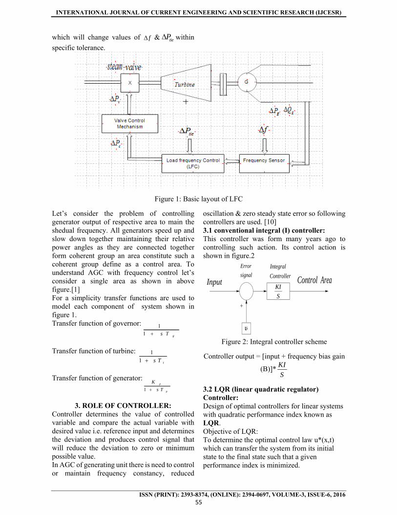
Figure 1: Basic layout of LFC

Let’s consider the problem of controlling generator output of respective area to main the shedual frequency. All generators speed up and slow down together maintaining their relative power angles as they are connected together form coherent group an area constitute such a coherent group define as a control area. To understand AGC with frequency control let’s consider a single area as shown in above figure.[1] For a simplicity transfer functions are used to model each component of system shown in figure 1. Transfer function of governor: 1

1 gs T

Transfer function of turbine: 1

1 ts T

Transfer function of generator:

1p

p

K

s T

3. ROLE OF CONTROLLER:

Controller determines the value of controlled variable and compare the actual variable with desired value i.e. reference input and determines the deviation and produces control signal that will reduce the deviation to zero or minimum possible value. In AGC of generating unit there is need to control or maintain frequency constancy, reduced

oscillation & zero steady state error so following controllers are used. [10] 3.1 conventional integral (I) controller: This controller was form many years ago to controlling such action. Its control action is shown in figure.2

KI

S

Input

Control Area

Error

signal

Integral

Controller

Figure 2: Integral controller scheme

Controller output = [input + frequency bias gain

(B)]*KI

S

3.2 LQR (linear quadratic regulator) Controller: Design of optimal controllers for linear systems with quadratic performance index known as LQR. Objective of LQR: To determine the optimal control law u*(x,t) which can transfer the system from its initial state to the final state such that a given performance index is minimized.



56

The PI is selected to give the best trade-off between performance and cost of control. The PI is widely used in optimal control design is known

as quadratic performance index and is based on minimum error and minimum energy criteria.

4. STATE SPACE ANALYSIS OF TWO SYSTEMS:

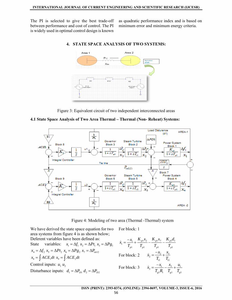
Figure 3: Equivalent circuit of two independent interconnected areas

4.1 State Space Analysis of Two Area Thermal – Thermal (Non- Reheat) Systems:

Figure 4: Modeling of two area (Thermal -Thermal) system

We have derived the state space equation for two area systems from figure 4 is as shown below; Deferent variables have been defined as: State variables: 1 1x f 2 1x Pt 3 1x Pg

4 2x f 5 2x Pt 6 2x Pg 7 12tiex P

8 1x ACE dt 9 2x ACE dt

Control inputs: 1u 2u

Disturbance inputs: 1 1Dd P 2 2Dd P

For block: 1

1 2 1 7 1 111

1 1 1 1

p p p

p p p p

K x K x K dxx

T T T T

For block: 2 322

1 1t t

xxx

T T

For block: 3 31 13

1 1 1 1g g g

xx ux

T R T T



57

For block: 4

5 2 7 2 2 244

2 2 2 2

p p p

p p p p

x k x k d kxx

T T T T

For block: 5 5 65

2 2t t

x xx

T T

For block: 6 64 26

2 2 2 2g g g

xx ux

T R T T

For block: 7 7 1 4 0( )2x x x T

For block: 8 8 1 1 7x x B x

For block: 9 9 4 2 7x x B x

Above equations are arranged in vector matrix which ate known as STATE EQUATION:

x Ax Bu d

1 2 3 4 5 6 7 8 9

Tx x x x x x x x x x

1

2

uu

u

1

2

dd

d

1 1

1 11

1 1

1 1 1

2 2

2 2 2

2 2

2 2 2

1

2

10 0 0 0 0 0

1 10 0 0 0 0 0 0

1 10 0 0 0 0 0 0

10 0 0 0 0 0

1 10 0 0 0 0 0 0

1 10 0 0 0 0 0 0

2 0 0 0 2 0 0 0 0 0 0

0 0 0 0 0 1 0 0

0 0 0 0 0 1 0 0

p p

p pp

t t

g g

p p

p p p

t t

g g

K K

T T T

T T

T R T

K K

A T T T

T T

T R T

T T

B

B

1

1

2

2

0

0 0

0 0

0

0 0

0 0

0 0

0 0

0 0

p

p

p

p

K

T

K

T

1

2

0 0

0 0

10

0 0

0 0

10

0 0

0 0

0 0

g

g

T

B

T

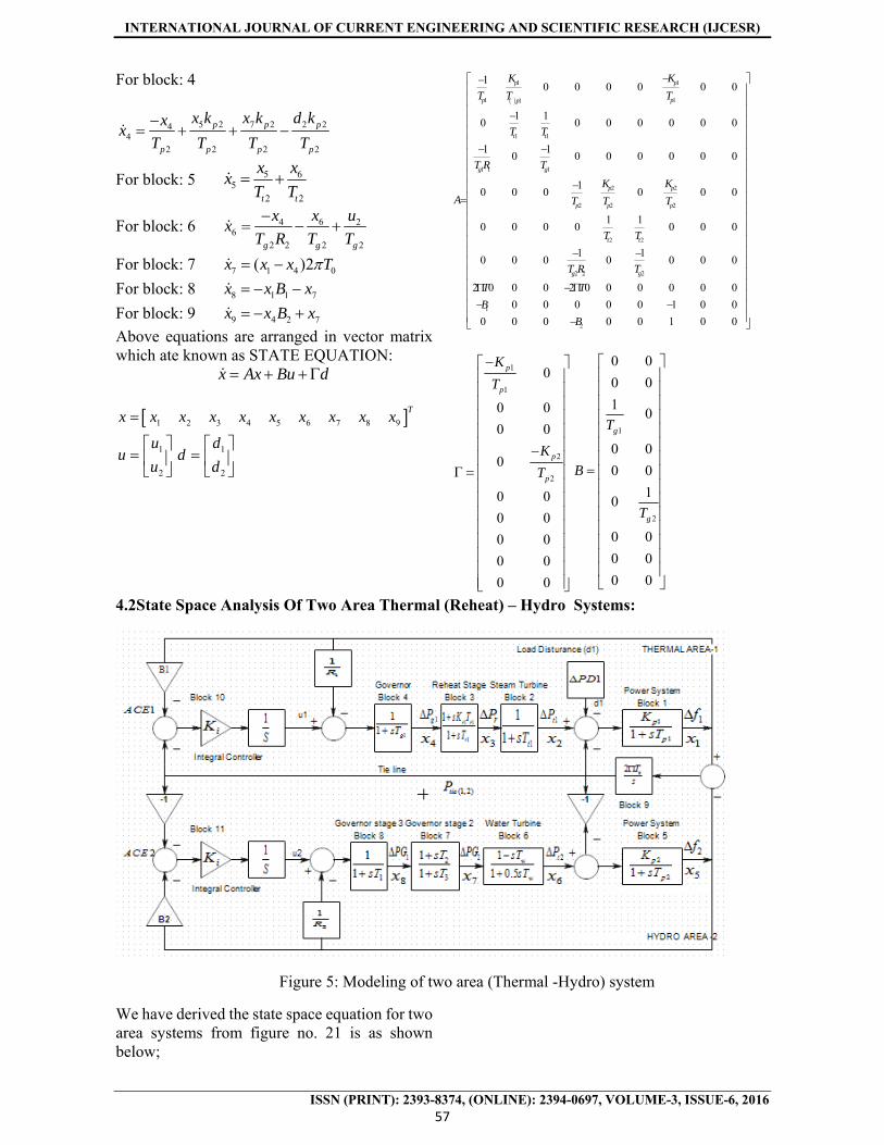
4.2State Space Analysis Of Two Area Thermal (Reheat) – Hydro Systems:

Figure 5: Modeling of two area (Thermal -Hydro) system

We have derived the state space equation for two area systems from figure no. 21 is as shown below;



58

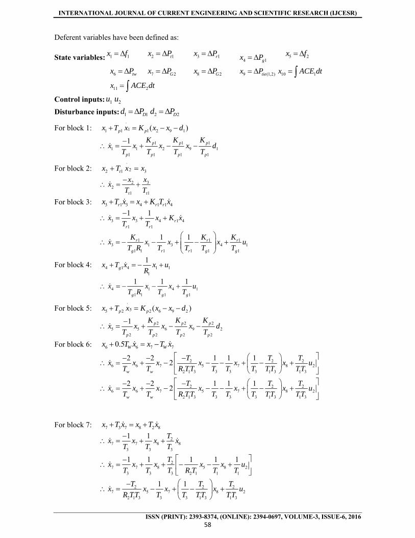
Deferent variables have been defined as:

State variables: 1 1x f 2 1tx P 3 1rx P 4 1gx P 5 2x f

6 twx P 7 2Gx P 8 2Gx P 9 (1,2)tiex P 10 1x ACE dt 11 2x ACE dt

Control inputs: 1u 2u

Disturbance inputs: 1 1Dd P 2 2Dd P

For block 1: .

11 1 1 2 9 1( )p px T x K x x d

1 1 11 1 2 9 1

1 1 1 1

1 p p p

p p p p

K K Kx x x x d

T T T T

For block 2: .

22 1 3tx T x x

2 32

1 1t t

x xx

T T

For block 3: 3 1 3 4 1 1 4r r rx T x x K T x

3 3 4 1 41 1

1 1r

r r

x x x K xT T

1 1 13 1 3 4 1

1 1 1 1 1 1

1 1r r r

g r r g g

K K Kx x x x u

T R T T T T

For block 4: 4 1 4 1 11

1gx T x x u

R

4 1 4 11 1 1 1

1 1 1

g g g

x x x uT R T T

For block 5: .

55 2 2 6 9 2( )p px T x K x x d

2 2 25 5 6 9 2

2 2 2 2

1 p p p

p p p p

K K Kx x x x d

T T T T

For block 6: 6 6 7 70.5 W Wx T x x T x

2 2 26 6 7 5 7 8 2

2 1 3 3 3 3 1 3 1 3

2 2 1 1 12

w w

T T Tx x x x x x u

T T R TT T T T TT TT

2 2 26 6 7 5 7 8 2

2 1 3 3 3 3 1 3 1 3

2 2 1 1 12

w w

T T Tx x x x x x u

T T R TT T T T TT TT

For block 7: 7 3 7 8 2 8x T x x T x

27 7 8 8

3 3 3

1 1 Tx x x x

T T T

27 7 8 5 8 2

3 3 3 2 1 1 1

1 1 1 1 1Tx x x x x u

T T T R T T T

2 2 27 5 7 8 2

2 1 3 3 3 1 3 1 3

1 1T T Tx x x x u

R TT T T TT TT



59

For block 8: 8 1 8 5 22

1x T x x u

R

8 5 8 22 1 1 1

1 1 1x x x u

R T T T

For block 9: 0 0

9 1 52 2x T x T x

For block 10: 10 1 1 9x B x x

For block 11: 11 2 5 9x B x x

Above equations are arranged in vector matrix which ate known as STATE EQUATION: x Ax Bu d

State vector 1 2 3 4 5 6 7 8 9 10

Tx x x x x x x x x x x

Where, A(9*9) state matrix and B (9*2) control matrix.

Control vector

In optimal control the control inputs are chosen as a linear combination of feedback from all nine system states 1 2 9( , , ........., )x x x as given below:

Where K (2*9) is a feedback gain matrix given by;

The system state equation is:

(For step load change of constant magnitude,

The output equation is,

1 1

1 1 1

1 1

1 1

1 1 1 1 1

1 1 1

2 2

2 2 2

2 2

2 1 3 3 1 3 3

2

2 1 3

10 0 0 0 0 0 0 0

1 10 0 0 0 0 0 0 0 0

1 10 0 0 0 0 0 0 0

1 10 0 0 0 0 0 0 0 0

10 0 0 0 0 0 0 0

2 22 2 2 20 0 0 0 0 0 0

10 0 0 0 0

P P

P P P

t t

r r

g t t g

g g

P P

P P P

w w

K K

T T T

T T

K K

T R T T T

R T T

K K

T T TA

T T

R T T T T T T T T

T

R T T

2

3 3 1 3

2 1 1

0 0

1

2

10 0 0

1 10 0 0 0 0 0 0 0 0

2 0 0 0 2 0 0 0 0 0 0

1

1

T

T T T T

R T T

T T

B

B

1

1

1

2

1 3

2

1 3

1

0 0

0 0

0

10

0 0

20

0

10

0 0

0 0

0 0

r

g

g

K

T

T

TB

T T

T

T T

T

1

2

uu

u

u Kx

11 12 13 14 15 16 17 18 19 10 1 11

21 22 23 24 25 26 27 28 29 20 2 11

k k k k k k k k k k kK

k k k k k k k k k k k

x Ax Bu

0d

y Cx Du



60

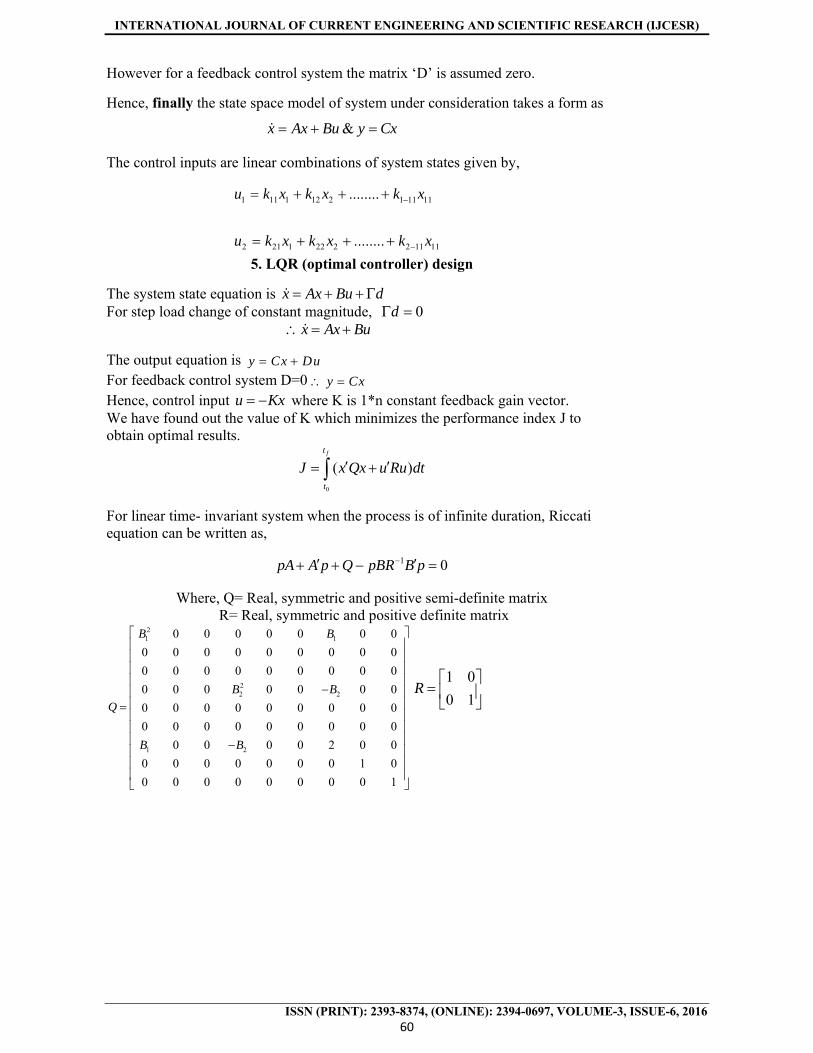
However for a feedback control system the matrix ‘D’ is assumed zero.

Hence, finally the state space model of system under consideration takes a form as

The control inputs are linear combinations of system states given by,

5. LQR (optimal controller) design

The system state equation is x Ax Bu d For step load change of constant magnitude, 0d x Ax Bu

The output equation is y Cx Du For feedback control system D=0 y Cx Hence, control input u Kx where K is 1*n constant feedback gain vector. We have found out the value of K which minimizes the performance index J to obtain optimal results.

0

( )ft

t

J x Qx u Ru dt

For linear time- invariant system when the process is of infinite duration, Riccati equation can be written as,

1 0pA A p Q pBR B p

Where, Q= Real, symmetric and positive semi-definite matrix R= Real, symmetric and positive definite matrix

21 1

22 2

1 2

0 0 0 0 0 0 0

0 0 0 0 0 0 0 0 0

0 0 0 0 0 0 0 0 0

0 0 0 0 0 0 0

0 0 0 0 0 0 0 0 0

0 0 0 0 0 0 0 0 0

0 0 0 0 2 0 0

0 0 0 0 0 0 0 1 0

0 0 0 0 0 0 0 0 1

B B

B B

Q

B B

1 0

0 1R

&x Ax Bu y Cx

1 11 1 12 2 1 11 11........u k x k x k x

2 21 1 22 2 2 11 11........u k x k x k x



61

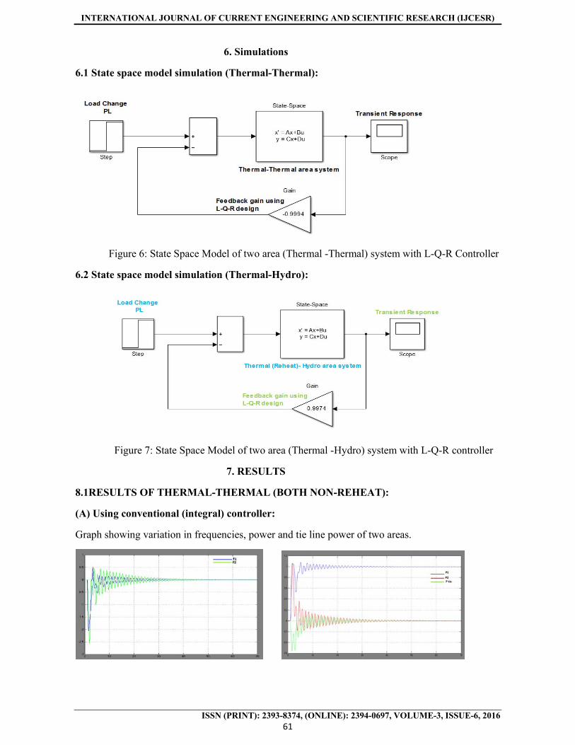
6. Simulations

6.1 State space model simulation (Thermal-Thermal):

Figure 6: State Space Model of two area (Thermal -Thermal) system with L-Q-R Controller

6.2 State space model simulation (Thermal-Hydro):

Figure 7: State Space Model of two area (Thermal -Hydro) system with L-Q-R controller

7. RESULTS

8.1RESULTS OF THERMAL-THERMAL (BOTH NON-REHEAT):

(A) Using conventional (integral) controller:

Graph showing variation in frequencies, power and tie line power of two areas.



62

(B) Using conventional (Proportional - integral) controller:

(C) Response of LQR from MATLAB simulink:

(D) By MATLAB programming:

Without L-Q-R With L-Q-R

(E) By state space modeling: (With LQR)



63

8.2 RESULTS OF THERMAL-THERMAL: (A) Using conventional (integral) controller: Graph showing variation in frequencies, power and tie line power of two areas.

(B) Using Conventional (Proportional - integral) Controller:

(C) Response of LQR from MATLAB simulink:

(D) By MATLAB programming:



64

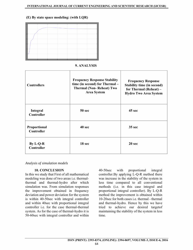
(E) By state space modeling: (with LQR)

9. ANALYSIS

Controllers

Frequency Response Stability time (in second) for Thermal – Thermal (Non- Reheat) Two

Area System

Frequency Response Stability time (in second) for Thermal (Reheat) –

Hydro Two Area System

Integral

Controller

50 sec

45 sec

Proportional Controller

40 sec

35 sec

By L-Q-R Controller

18 sec

20 sec

Analysis of simulation models

10. CONCLUSION In this we study that First of all mathematical modeling was done of two areas i.e. thermal-thermal and thermal-hydro after which simulation was. From simulation responses the improvement obtained in frequency deviation and power deviation for the system is within 40-50sec with integral controller and within 40sec with proportional integral controller i.e. for the case thermal-thermal system. As for the case of thermal-hydro it is 50-60sec with integral controller and within

40-50sec with proportional integral controller.By applying L-Q-R method there was increase in the stability of the system in less time compared to all conventional methods (i.e. in this case integral and proportional integral controller). By L-Q-R method the improvement is obtained within 10-20sec for both cases i.e. thermal - thermal and thermal-hydro. Hence by this we have tried to achieve our desired targetof maintaining the stability of the system in less time.



65

11.APPENDIX

10.1 For Thermal-Thermal (Both Non-Reheat):

PARAMETERS NOTATION AREA 1 (THERMAL)

AREA 2 (THERMAL)

Power System Gain Constant PSK 120 120

Power System Time Constant PST (sec) 20 20

Speed Regulation R (Hz/Mw) 2.5 2.5

Normal frequency f (Hz) 50 50

Governor time constant gsT (sec) 0.04 0.04

Turbine time constant tsT (sec) 0.5 0.6

Integrator constant iK 0.4 0.4

Frequency- Sensitive load coefficient. D (Mw/Hz) 0.00834 0.00834

10.2 For Thermal (Reheat)-Hydro:

PARAMETERS NOTATION AREA 1 (THERMAL)

NOTATION AREA 2 (Hydro)

Power System Gain Constant 1PSK

120 2PSK 120

Power System Time Constant 1PST (sec)

20 2PST 20

Speed Regulation 1R (Hz/Mw) 1.2

2R 1.2

Normal frequency 1f (Hz)

50 2f 50

Governor time constant 1gsT (sec) 0.08 1

2

3

T

T

T

0.3

5

28.75

Turbine time constant 1tT (sec)

1rT (sec)

0.3

10

0.2

Tw 0.3



66

1rK (sec)

Integrator constant 1iK

1 2iK 1

Frequency- Sensitive load coefficient.

1D (Mw/Hz) 0.0085 2D (Mw/Hz) 0.0085

Frequency bias constant 1B 0.8417

2B 0.8417

REFERENCES 1. IOSR Journal of Engineering

The State Space Modeling of Single, Two and Three ALFC of Power System Using Integral Control and Optimal LQR Control Method (Nilaykumar N. Shah, Chetan D. Kotwal)

2. State Space Modeling of load frequency control for multi area system by Krishna Pal Singh Parmar (IIT Report)

3. International Journal of Advanced Research in Electrical, Electronics and Instrumentation Engineering (IJAREEI),LQR Based Load Frequency Controller for Two Area Power System by K.Vasu and P.BhavanaV.Ganesh.

4. POWER SYSTEM ANALYSISbY HADI SAADAT (TATA MC GRAW HILL)

5. POWER SYSTEM STABILITY AND CONTROLbY PRABHA KUNDUR. (TATA MC GRAW HILL)

6. IJRET (International Journal of Research

in Engineering and Technology) RESEARCH PAPER.

7. ELECTRICAL POWER SYSTEM ESSENTIAL by Peter Schavemaker, Lou Vander Sluis.

8. POWER SYSTEM OPERATION AND CONTROL by R.V. Ramana

9. C.B. BANGAL book for power system. 10. Automatic Generation Control Of

Interconnected Hydrothermal Power Plant Using Classical And Soft Computing Technique By IJREA (international journal of engineering research and application)

11. AshutoshBhadoria, DhananjayBhadoria.

AUTOMATIC LOAD FREQUENCY CONTROL OF TWO …troindia.in/journal/ijcesr/vol3iss6/54-66.pdf · issn...

Documents

Transcript of AUTOMATIC LOAD FREQUENCY CONTROL OF TWO …troindia.in/journal/ijcesr/vol3iss6/54-66.pdf · issn...