See discussions, stats, and author profiles for this publication at: https://www.researchgate.net/publication/311971772

Automatic generation of second-level space boundary topology from IFC

geometry inputs

Article  in  Automation in Construction · December 2016

DOI: 10.1016/j.autcon.2016.08.044

CITATIONS

30READS

1,083

3 authors:

Some of the authors of this publication are also working on these related projects:

Positive Energy Buildings thru Better controL dEcisions (PEBBLE) View project

H2020 OptEEmAL - Optimized Energy Efficient design platform for refurbishment At district Level View project

Georgios Nektarios Lilis

University College London

42 PUBLICATIONS   217 CITATIONS   

SEE PROFILE

Georgios I. Giannakis

Technical University of Crete

48 PUBLICATIONS   219 CITATIONS   

SEE PROFILE

Dimitrios Rovas

Technical University of Crete

91 PUBLICATIONS   1,849 CITATIONS   

SEE PROFILE

All content following this page was uploaded by Georgios Nektarios Lilis on 20 February 2018.

The user has requested enhancement of the downloaded file.

Automatic generation of second-level space boundary topology from

IFC geometry inputs

Abstract

The Industry Foundation Classes (IFC) is a semantically rich data model providing nec-essary information to support extraction of information necessary for the setup of buildingenergy simulations. Often, 2nd-level space boundary data contained in IFC, are missing orincorrect. To facilitate the connection between BIMs and energy simulation programs, theCommon Boundary Intersection Projection (CBIP) algorithm is introduced. CBIP uses thegeometric representations of building entities obtained from IFC files to generate the building’s2nd-level space boundary topology. A prototypical implementation of the CBIP algorithm isused in a complex geometry building, as a verification of the capability of the algorithm toidentify space boundaries.

Keywords: Industry Foundation Class, Building Information Model, Building EnergyPerformance Simulation, Second-level Space Boundaries

Introduction

The recent requirement for efficient allocation of energy resources in the building sector,has resulted in the increased use of building thermal simulations, during both the buildingdesign [1, 2] and operation phases [3, 4]. The accuracy of a thermal simulation model stronglydepends on the accurate definition of building geometric characteristics, which include: thebuilding envelope, the building orientation, the configuration of spaces, surfaces and volumes.

In current state of practice, it is quite common that a Computer-Aided Design (CAD) toolis used to represent the geometry. However, such an architectural perspective must be altered,in order for energy simulations to be performed [5]. Hence, building geometrical data extractedfrom CAD programs have to be manually transformed and combined with material propertiesto be entered as inputs to energy simulation routines, a process which is both time consumingand error-prone. CAD data have simple semantics, Building Information Models (BIM) [6]provide an improved way for information storage with richer semantics that include: buildinggeometry, material data and information on building services. Open BIM data schemas includethe Industry Foundation Classes (IFC) [7] and the green-building XML schema (gbXML) [8].The popularity of these two open BIM schemas led many leading AEC software companies toimplement support for gbXML- and IFC-based exchanges within their BIM authoring suites.Examples of such tools are Revit (AutoDesk) [9] and ArchiCad (GraphiSoft) [10].

A wide variety of promising attempts have been proposed to establish an automated dataexchange between BIM and thermal simulation tools. The IDF Generator [11], developed atthe Lawrence Berkeley National Laboratory (LBNL), works in conjunction with the Geome-try Simplification Tool (GST) and transforms IFC-format building geometry into EnergyPlusinput-data file (IDF) [12]; GST simplifies the original building geometry defined in IFC-formatand converts it into gbXML-format, while the IDF Generator converts the gbXML-format fileinto EnergyPlus input-data file. The resulting IDF file contains all information related to

Preprint submitted to Automation in Construction January 19, 2017

building geometry and constructions needed to run an EnergyPlus simulation. IDF Generatoris proposed as a semi-automated process, since for complex building geometries a manual ma-nipulation of IDF geometry is required, including some corrections to windows in curtain walls,missing floors and ceilings [13]. The RIUSKA [14], developed by Granlund, uses the DOE-2.1[15] thermal simulation engine and imports the building geometry from an IFC file, utilizingthe BSPro server middleware ([16]). Limitations of its IFC import exist, since RIUSKA ignoresslabs in the IFC file and simply generates them internally, according to the size of the spacedefined by the bounding walls. Moreover, high quality of import results are achieved only whenRIUSKA is used in conjunction with SMOG, while compatibility problems occur when otherCAD tools are used to author and export the IFC file.

In the AEC software industry, Green Building Studio (GBS) [17] web service uploads thegeometry in gbXML-format and converts it into a DOE-2.2 or an EnergyPlus-format file. Thereare studies proving that several problems occur during the conversion process [18], includingincorrect shading surface definitions and omission of some walls. Trimble’s SketchUp togetherwith its Openstudio and IFC2SKP plugins, is able to upload any gbXML or IFC well-formattedgeometry and convert it into the EnergyPlus or TRNSYS17-format file [19]. However, lack ofmaturity of the import tool, neglects some information related to floors and ceilings. VirtualEnvironment (VE), developed by Integrated Environmental Solutions (IES) [20], is an inte-grated system that uses its own simulation engine, called Apache. IES VE supports import ofgbXML and IFC file formats. Nevertheless, import results rely on the correctness of 2nd-levelspace boundary geometry contained in IFC, which currently is not exported properly by anyBIM authoring tool.

Among the two most popular BIM schemes, gbXML and IFC, IFC appears to be a suitablechoice as its more rich in content, enables interoperability among different software environ-ments and can be updated according to the building’s modifications [21].

Concerning the building geometry, IFC can provide static building information that includegeometric configuration and material properties, but in a form that might not be directly usablefor the generation of thermal simulation models due to the absence of 2nd-level space bound-ary information [13]. Hence, a consistent approach is required to extract building geometryinformation, contained in an IFC file, and subsequently to correctly identify the 2nd-level spaceboundary information.

In view of this, several algorithms have been proposed [22],[23], [24], which are based ongraph theory and convert a three-dimensional architectural building model into the second-levelspace boundary topology without the need for definition of conditioned building space volumes.

In this work, following a different approach to address the 2nd-level space boundary gen-eration requirement, the Common Boundary Intersection Projection (CBIP) algorithm is pre-sented. A recent study has shown that thermal models obtained based on CBIP algorithmresults, are comparable to models of other popular programs [25, 26].

CBIP algorithm can be applied to building geometries which do not contain design errors orbuilding space incorrect definitions. In [27], errors that affect the creation of properly defined2nd-level space bounaries are presented. Commercial software, such as Solibri Model Checker,[28] are able to identify such errors, which are communicated back to the AEC software andcorrected manually. With an IFC free of design errors and building space incorrect definitionsat hand, its geometric data can be used as input to CBIP algorithm.

Algorithmically, CBIP is divided into four operational stages: the Identification (ID) stage,the Boundary Surface Extraction (BSE) stage, the Common Boundary Intersection (CBI) stageand the Boundary Intersection Projection (BIP) stage which are analysed in Section 4. CBIP’sstages involve geometric operations based on well-known methods for representing shapes, there-

2

fore an initial description of such methods, adopted by the algorithm, are presented in Sections2 and 3. The output of the algorithm used to update the IFC database and the respectiveSpace Boundary class, is described in Section 5, while design requirements and design recom-mendations to ensure the correct execution of the algorithm are discussed in Sections 6 and 7,respectively. Finally, CBIP has been tested on a demonstration building of a high geometrycomplexity and its results are presented in Section 9.

CBIP algorithm – Geometric Definitions

CBIP takes as input the geometric representations of various building entities, which are as-sumed to be polyhedrons, performs certain operations on them and outputs polygonal surfaceswhich are the 2nd-level space boundaries. Consequently, CBIP algorithm’s mathematical foun-dation consists of geometric operations, applied on geometric representations of the involvedbuilding entities.

Various geometric representation methods including the octree and the Boundary represen-tation have been used in Building Information Models [29]. In CBIP two such methods areused. The first, is the Boundary representation (B-rep) [30], described in Section 2.1. B-reptheory is adopted in order to describe each polyhedron by its corresponding boundary polygons.Additionally, to determine the space boundaries which are essentially common surfaces sharedby two polyhedrons, the Binary Space Partitioning tree (BSP-tree) polyhedral representation[31] is adopted and described in Section 2.2.

Boundary representation

The B-rep of a polyhedron A associated with a building entity, is denoted by ∂A. Essen-tially, ∂A is a set of boundary polygon surfaces ∂A = {A1, ..., Ai, ..., AN} (see figure 1). Eachboundary polygon surface in this representation, conforms to the right hand outward normalconvention: the direction of the normal vector nAi

of every boundary polygon Ai evaluatedusing the right hand, is towards the exterior of the polyhedron A, as displayed in figure 1. Theright hand normal vector direction evaluation method proceeds as follows: when the fingers ofthe right hand, excluding the thumb, follow the points of the polygon Ai, the thumb pointsto the direction of the normal vector. Consequently, the outward normal convention, withthe direction of the normal vectors evaluated using right hand, requires the boundary polygonpoints to be correctly ordered: in a counter clock-wise manner when looking from outside thepolyhedron (as displayed in figure 1).

Boundary of polyhedron Boundary polygon

Normal vector direction calculated using the thumb of the right hand. ...

Figure 1: Boundary representation (B-rep) of a polyhedron as a set of boundary polygon surfaces ∂A ={A1, ..., Ai, ..., AN}. When the points of each polygon surface Ai are correctly ordered (counter clockwise whenlooking from outside the polyhedron) the direction of the normal vector of the surface nAi

, evaluated using theright hand, is towards the exterior of the polyhedron.

3

Binary Space Partitioning tree representation

A Binary Space Partitioning tree representation or BSP-tree refer generally to a set ofsurfaces A and is denoted by TA. Since most of the surface sets encountered here are B-reps,the respective BSP-trees refer to polyhedrons A and are denoted by TA, instead of T∂A forsimplicity.

An example of a BSP-tree referring to an intersection surface set AI ⊂ ∂A of a polyhedronA, is displayed in figure 2. In a broad sense, TA contains the boundary polygons of ∂A anddefines a partition of the 3D space into a finite set of sub-spaces, depending on the orientation ofthe polyhedron’s boundary surfaces. In a broad sense, a BSP-tree of a polyhedron is a binarytree that partitions the 3D space into finite number of sub-spaces according to the outwardnormal vectors of its boundary surfaces, as described below.

TA is a structure with three fields. The root value of a BSP-tree TA contains a single-rootpolygon, or multiple-root coplanar polygons with identical normal vectors, and is denoted bythe pol field (TA.pol). The plane of the root divides the 3D space into two sub-spaces, theoutside and the inside sub-space. The outside sub-space is indicated by the common normalvector of the root polygon(s). The outside sub-space contains polygons which are placed in theright sub-tree of TA and is denoted by the field TA.out. The inside sub-space is indicated by theopposite of the normal vector of the root polygon(s). The inside sub-space contains polygonswhich are placed in the left sub-tree of TA, and is denoted by the field TA.ins.

Consequently, moving from the root to the leaves of the tree and following the left/rightbranches lead to inside/outside sub-spaces (opposite/towards the direction of the outward nor-mal vectors), respectively. The final partitions (sub-regions) of the 3D space are indicated bythe leaves of the tree which contain binary values. By convention, a leaf has value 1, if therespective sub-region is inside the polygons of the node above the leaf, and the value 0, if therespective subregion lies outside these polygons.

B-rep of polyhedron BSP-tree representation

0Subspace

0Subspace

0Subspace

1Subspace

1Subspace

1Subspace

0Subspace

1

2

3

7

1

2

3

7

4

5 6

4

5

6

Polyhedron intersection

Figure 2: BSP-tree representation of an intersection surface set AI = {A1, ..., A7} ⊂ ∂A of a polyhedron Acreating a non-convex region.

If two boundary polygons are coplanar but their outward normal vectors have oppositedirections, one polygon is considered to lie outside the other and therefore are placed in separateroot nodes. The sequence of the boundary polygons of ∂A, used to populate the BSP-tree TA,does not matter. The tree representation TA of a polyhedron A is obtained from its B-reprepresentation ∂A using the recursive algorithm described in [31].

4

CBIP algorithm – Geometric operations

To obtain the 2nd-level space boundary surfaces, which are parts of common boundarysurfaces between the polyhedral representations of building spaces and the polyhedral rep-resentations of building constructions, CBIP performs geometric operations defined by threegeometric clipping functions. These clipping functions are applied on polyhedral pairs A, B,and use: (1) their B-reps ∂A = {A1, ..., AN∂A

}, ∂B = {B1, ..., BN∂B}, with N∂A, N∂B the

cardinalities of the sets ∂A, ∂B; (2) the respective BSP-tree representations TA, TB; (3) twopolygon clipping operators c1 and c2; and (4) a polygon set partition function.

Polygon clipping operators

Polygon clipping operators c1 and c2 involve two polygons Ai and Bj. Essentially, c1 andc2 modify their second operand (polygon Ai), depending on the relative position of their firstoperand (polygon Bj) and the direction of its normal vector nBj

(see figure 3).Mathematically, these operations are defined by:

A1i = Bj(c1)Ai and A2i = Bj(c2)Ai (1)

Generally, three clipping cases can be distinguished:

A. The plane of Bj dissects Ai into two parts: A1i towards the normal vector nBjand A2i

towards the opposite direction −nBj. This dissection is performed by c1 or c2, returning

A1i or A2i, respectively (Ai = A1i ∪ A2i).

B1. The plane of Bj dissects the plane of Ai into two half-planes and Ai is in the half-spacepointed by nBj

. In this case c1 returns Ai and c2 returns an empty set.

B2. The plane of Bj dissects the plane of Ai into two half-planes and Ai is in the half-spacepointed by −nBj

. In this case c1 returns an empty set and c2 returns Ai.

The previous clipping operations are implemented using 2D set operations on polygons(intersection, union and subtraction), following the algorithm proposed in [32].

5

Common Line

POLYGON B (clipping polygon)

POLYGON A (clipped polygon)

i

GENERAL CASE – A (Polygon is split by polygon )

SPECIAL CASE – B1 (Polygon is in half-space pointed by )

A = A1i i

`

A = { } 2i

Bn j

A 1i

A 2i

Bn j

An i

B j iA

iA

B j

1iA

2iA 2iA

1iA

An i

Bn j

Bn jPOLYGON B (clipping polygon)

POLYGON A (clipped polygon)

SPECIAL CASE – B2 (Polygon is in half-space pointed by ) B-n j iA

POLYGON A (clipped polygon)

POLYGON B (clipping polygon)

B j

i

i

j

j

j

Bn j

Bn j

B-n j

B j

An i

Bn j

An i

A = { }1i

A = A 2i i

An i

An i

Figure 3: Illustration of polygon clipping operators c1 and c2 on polygon Ai by polygon Bj .

Polygon set partition function

The polygon set partition function P , used by the geometric clipping functions, can bedefined as a partition of a polygon set A, intersected by a set of coplanar polygons (partitionset B) with the same outward normal vector nB (see figure 4).

6

Coplanar polygon set (clipping)

Polygon set (clipped)

Normal vector of a boundary surface of clipping polygon set

Normal vector of a boundary surface of clipped polyhedron

Inside

Outside

Figure 4: Illustration of the polygon set partition function

Mathematically, the polygon set partition function P is defined by the following expression:

[Ains, Acsd, Acod, Aout] = P (B,A) (2)

The returning arguments Ains and Aout are subsets of the set A containing polygons lying inthe half-space pointed by −nB and nB, respectively. Acop and Acsd contain polygons coplanarwith the polygons in B, which have opposite (cod) and same direction (csd) normals with nB,respectively (see figure 4). The above sets are populated using Algorithm 1 and the polygonclipping operators c1 and c2.

Polygon set clipping functions

Using the operators c1, c2, and the polygon partition function P , three recursive clippingfunctions Fins, Fout and Fcod are defined. These functions are applied on a polygon setA (clippedpolyhedron), using the BSP-tree representation TB of a polyhedron B (clipping polyhedron).These clipping functions return:

Algorithm 1 Partition function P (B,A)

A = {A1, ..., AN} // Polygon set (to be partitioned) //B = {B1, ..., BM} // Polygon set (partitioning set) //Ains = ∅, Acsd = ∅, Acod = ∅, Aout = ∅ // Initialize output sets //for i = 1 : N do

if Ai ∈ A, B1 are coplanar thenfor j = 1 : M do

Ai ← Ai −Bj // Subtract Bj from Ai and update Ai //AIBij = Ai ∩Bj // Intersect Bj with Ai and form AIBij polygon //if nAi

↑↑ nBjthen

Acsd ← Acsd ∪AIBij // Include polygon AIBij in Acsd set //elseAcod ← Acod ∪AIBij // Include polygon AIBij in Acod set //

end ifend forAout ← Aout ∪Ai // Include polygon Ai in Aout set //

elseAins ← Ains ∪ [B1(c2)Ai] // Include clipped polygon [B1(c2)Ai] in Ains set //Aout ← Aout ∪ [B1(c1)Ai] // Include clipped polygon [B1(c1)Ai] in Aout set //

end ifend for

7

• Ains = Fins(TB,A): The parts of A, which are inside polyhedron B;

• Aout = Fout(TB,A): The parts of A, which are outside polyhedron B;

• Acod = Fcod(TB,A): The parts of A, which are coplanar with the surfaces of ∂B and haveopposite outward normal vectors.

Function Fins is described by Algorithm 2, function Fout by Algorithm 3 and function Fcod

by Algorithm 4. In these algorithms, the clipping BSP-tree TB has three fields: TB.pol refersto the polygons contained in the root of TB; TB.ins contains the left (inside) sub-tree of TB;and TB.out contains the right (outside) sub-tree of TB.

The Fcod function is used by CBIP to identify the Common Boundary Intersection surfaces,which are coplanar surface pairs belonging to two different polyhedrons and have oppositenormal vectors. Examples of the clipping functions Fout, Fins and Fcod, applied on A, using aclipping polyhedron B are displayed in figure 5.

Polyhendron B(clipping)

Surface set (clipped)

Normal vector of a boundary surface of clipping polyhedron.Normal vectors of a surfaces of the clipped boundary set.

Figure 5: Results of clipping functions – A is the polygon set of a clipped polyhedron and B is the clippingpolyhedron

Algorithm 2 Inside clipping function Fins: Ains = Fins(TB,A)

if TB is binary thenif TB = 0 thenAins = ∅ // Initialize output set Ains //

end ifif TB = 1 thenAins = A // Initialize output set Ains with A //

end ifelse

[Ains, Acsd, Acod, Aout] = P (TB.pol,A) // Partition A with TB.pol //if Ains 6= ∅ thenAi,ins = Fins(TB.ins,Ains) // Apply Fins recursively on Ains with TB.ins //Ains ← Ains ∪ Ai,ins // Include Ai,ins in Ains //

end ifif Aout 6= ∅ thenAi,out = Fins(TB.out,Aout) // Apply Fins recursively on Aout with TB.out //Ains ← Ains ∪ Ai,out // Include Ai,out in Ains //

end ifend if

8

Algorithm 3 Outside clipping function Fout: Aout = Fout(TB,A)

if TB is binary thenif TB = 0 thenAout = A // Initialize output set Aout with A //

end ifif TB = 1 thenAout = ∅ // Initialize output set Aout //

end ifelse

[Ains, Acsd, Acod, Aout] = P (TB.pol,A) // Partition A with TB.pol //if Ains 6= ∅ thenAo,ins = Fout(TB.ins,Ains) // Apply Fout recursively on Ains with TB.ins //Aout ← Aout ∪ Ao,ins // Include Ao,ins in Aout //

end ifif Aout 6= ∅ thenAo,out = Fout(TB.out,Aout) // Apply Fout recursively on Aout with TB.out //Aout ← Aout ∪ Ao,out // Include Ao,out in Aout //

end ifend if

Algorithm 4 Coplanar opposite direction clipping functionFcod: Acod = Fcod(TB,A)

if TB is a tree (not binary value) then[Ains, Acsd, Acod Aout] = P (TB.pol,A) // Partition A with TB.pol //if Acod 6= ∅ thenAcod ← Acod // Initialize output set Acod //

end ifif Ains 6= ∅ thenAc,ins = Fcod(TB.ins,Ains) // Apply Fcod recursively on Ains with TB.ins //Acod ← Acod ∪ Ac,ins // Include Ac,ins in Acod //

end ifif Aout 6= ∅ thenAc,out = Fcod(TB.out,Aout) // Apply Fcod recursively on Aout with TB.out //Acod ← Acod ∪ Ac,out // Include Ac,out in Acod //

end ifend if

CBIP algorithm stages

As mentioned earlier, CBIP consists of four operational stages. CBIP’s input contains IFCgeometric data related to three types of building entities: Constructions, Openings and Vol-umes. The final output of the CBIP process is the generation of the 2nd-level space boundaries,which are essentially surface pairs, associated with four types of thermal simulation elements.

The input data of CBIP are gathered in the first stage. Their classification to Constructions,Openings and Volumes is performed according to their roles in a thermal simulation process.The first stage is described in Section 4.1.

The scope of the second stage, is to generate the B-reps of the building entities, isolatedfrom the first stage. This is accomplished using a process called Boundary Surface Extraction(BSE), described in Section 4.2. In some cases, building entities of the Construction typemay contain entities of the Opening type, for instance building walls (Constructions) whichcontain doors or windows. In such cases, the B-reps of these constructions have to be updated

9

by subtracting the B-reps of the opening volumes, they contain. This is performed by theOpening Construction Subtraction (OCS) process, described in Section 4.2.1.

The boundary surfaces’ B-reps, deduced from the second stage, are processed further in thethird stage, where the Common Boundary Intersection (CBI) process (described in Section 4.3)is applied to obtain the Common Boundary (CB) surfaces shared by B-rep pairs. CB surfaces’types are denoted as Primary types and are described in Section 4.3.1. The remaining B-repsurfaces, which are not CB surfaces, are also gathered using the Remaining Surface Extraction(RSE) process (described in Section 4.3.2), and are marked as Derived types of surfaces, whichare attached to the environment.

Finally, the 2nd-level space boundary surfaces, the associated four types of thermal simu-lation model elements (thermal, shades, openings and air boundaries) and their connectivityinformation are obtained in the fourth stage. This is accomplished by projection of a CB surface(first surface), obtained from the third stage, to the plane of another CB surface (second sur-face) and vice versa. This process, called Boundary Intersection Projection (BIP), is describedin Section 4.4.

Identification stage - ID (stage 1)

Even though IFC files contain information referring to multiple building geometry entities,only some of them are required for building thermal simulations. These building geometryentities can be classified into three categories depending on their role in thermal buildingsimulations: Constructions, Openings and Volumes.

Constructions are single- or multi-layer entities, which are involved in thermal simulationsin two different ways: (1) directly, by impeding thermal energy flow between building volumes,where the construction layers and their specific thermal properties are taken into account;and (2) indirectly, by blocking sunlight, thus impeding solar heat gains (shading), where theirthermal behavior is not considered. Certain IFC classes, which refer to building constructions,belong to the abstract IfcBuildingElement class and are indicated by the “CONSTRUCTIONS”dashed rectangle in figure 7.

Openings are building entities described by the IfcOpening class. These entities containdoors, windows and skylights, which are generally holes on building Constructions. Theseentities play important role in thermal simulations, since depending on their state either impedeor allow thermal flow. The IfcOpeningElement class contains information associated withbuilding openings and belongs to the abstract IfcElement class. This class and its relations areindicated by the “OPENINGS” dashed rectangle in figure 7.

Building volumes are entities that exchange thermal energy, which are categorized as follows:

• Building spaces refer to the air volumes of rooms or room partitions (separated by airboundaries). Building spaces interchange thermal energy with other spaces, with thesurrounding environment or with the site encompassing the building. Building spaces aredefined by the IfcSpace class.

• Building site refers to the surrounding ground volume, encompassing the building underconsideration. The building site is defined by the IfcSite class.

IFC classes related to Volume entities, belong to the abstract IfcBuildingSpatialStructureEle-ment class and are indicated by the “VOLUMES” dashed rectangle in figure 7.

The aforementioned building entities are extracted and their polyhedral boundary surfacerepresentations are obtained from their boundary surfaces, as described in Section 4.2.

10

Boundary Surface Extraction stage - BSE (stage 2)

In IFC, all relative building entities, required for the execution of CBIP, are consideredproducts which are related to the abstract IfcProduct class. All associated products have a3D shape representation, condition which is met by the Design Transfer View definition [33],as figure 7 indicates. However, an essential input requirement of CBIP algorithm, is that allinvolved products must have an outward oriented boundary surface geometric representation(B-rep), as described in Section 2.1, condition which is not always satisfied. Hence, furtherprocessing on some products’ shape representations is required to obtain the desired B-reps.The required data for the generation of the B-reps are contained in the IfcGeometricRepresen-tationItem class, related to the IfcProductDefinitionShape subclass of the IfcProduct class (seefigure 7).

There are five main solid geometrical representations and respective sub-classes of the IfcGe-ometricRepresentationItem class, according to figure 7. The involved geometric representationsand the respective IFC classes, contained in Design Transfer View 1.0 [33], are:

(1) Face based surface model representation, described by IfcBasedSurfaceModel class – Ac-cording to this representation, the solid of the building entity is described by a set ofboundary surfaces “faces” in a 3D space. Such representation need no further processingand can be used directly by the CBIP algorithm, provided that the surfaces are correctlyoriented.

(2) Solid model representation, described by IfcSolidModel class – This class consists of fivesubclasses referring to the way the solid model is being represented:

• Manifold solid representation, described by IfcManifoldSolidBrep class – A manifoldsolid B-rep is a finite, arc-wise connected volume bounded by one or more surfaces,each of which is a connected, oriented, finite, closed 2D-manifold. In this case nofurther processing is required, since all the points of the boundary surfaces are given.

• Swept area solid representation, described by IfcSweptAreaSolid class – This classcontains solids, either described by a 2D profile being extruded towards a given direc-tion and length (IfcExtrudedAreaSolid), or revolved around a fixed axes (IfcRevolvedAr-eaSolid), or translated along a curve trajectory (IfcSurfaceCurvedSweptAreaSolid).

In this case, based on the base profile points, the extrusion direction and the extru-sion length, the remaining points of the boundary surfaces are calculated and therespective boundary polygons are obtained. Essentially, the obtained base pointsare being translated or rotated (depending on the case) following a certain direction,generating the rest boundary surface points.

(3) Half Space Solid representation, described by IfcHalfSpaceSolid class – Two cases of half-space solid representation can be distinguished:

• Polygonal bounded half-space representation – the half space solid is bounded by abase polygon that is extruded at a specific depth and is intersected by a 3D surface(plane or curved surface in general). As in the case of the extruded area solid, thepoints of the boundary surfaces are obtained from the base points, the extrusiondirection and length, and the intersecting surface.

• Boxed half-space representation – similarly to the polygonal bounded half-space solid,it is bounded by a bounding box. In this case the points of the bounding boxdetermine the points of the intersecting boundary surfaces.

11

(4) Boolean result representation, described by IfcBooleanResult class – This class refers tosolid geometric representations, which are obtained by performing boolean operations(union, intersection, difference) on solids, represented by the previous classes. Conse-quently the B-reps of all the involved solids are extracted and the final results are obtainedby the clipping functions, applied on the extracted B-reps.

Representations that do not contain the desired B-reps for CBIP, require geometric calcula-tions. These calculations are preformed in the second stage of the Boundary Surface Extraction(BSE) process. The sub-classes, data of which require geometric calculations to obtain therespective B-reps, are indicated by dashed blocks in the Express-G diagram of figure 7.

Opening Construction Subtraction process (OCS)

Constructions containing openings are represented in IFC files as solid objects, withoutconsidering the openings as holes. Therefore, to obtain a more accurate B-rep of these con-structions and to determine the common boundary surfaces among these constructions andtheir opening volumes (frames of doors, windows, etc.), the polyhedral geometrical represen-tations of the opening volumes must be subtracted from the polyhedral representations of theconstructions. Such subtraction is performed by the Opening Construction Subtraction (OCS)process, which uses the Fins and Fout clipping functions, given as inputs: the B-rep ∂A, theBSP-tree representation TA of the construction A, the B-rep ∂Aop and BSP-tree representationTAop of the union of its openings ∂Aop: ∂Aop = ∂O1 ∪ ... ∪ ∂ON (∂Oi is the B-rep of openingi).

OCS process returns a set of boundary polygons (B-rep) of the construction with its openingssubtracted. OCS is illustrated in figure 6, for the case of a wall containing a door and a window.

ExternalWall

Openings

OpeningSubtraction

Figure 6: Illustration of OCS process applied on a rectangular, wall containing door and window openings

Mathematically, OCS process is described as follows:

OCS(TA, ∂A, TAop , ∂Aop) =⋃ Fout(TAop , ∂A)

Fcod(TAop , ∂A)Fins(TA, ∂Aop)

−1

(3)

The exponent −1, applied to Fins function, inverts the ordering of the points of the obtainedpolygons, which also inverts their normal vectors.

12

IfcFaceBasedSurfaceModel

IfcSolidModel(ABS)

IfcBooleanResult

IfcHalfSpaceSolid

IfcGeometricRepresentationItem(ABS)

1

IfcRepresentationItem(ABS)

IfcRepresentation

1

1

IfcProductRepresentation

IfcProductDefinitionShape

1

IfcProduct(ABS)

IfcObject(ABS)

1

IfcElement(ABS)

IfcSpatialStructureElement(ABS)

IfcBuildingElement(ABS)

IfcWall

IfcSlab

IfcCovering

IfcBuildingElementProxy

IfcBeam

1

IfcColumn

IfcRoof

IfcCurtainWall

1

IfcSpace

IfcSite

1

1

PRODUCT DEFINITION SHAPE

IfcRelFillsElement IfcOpeningElement

RelatingOpeningElement

(INV) HasFillings S[0.?]

RelatedBuildingElement

(INV) FillsVoids S[0.?]

CONSTRUCTIONS

VOLUMES

OPENINGS

IfcManifoldSolidBrep (ABS)

IfcSweptAreaSolid(ABS)

IfcExtrudedAreaSolid

1

1

= Class which requires geometric calculations

Figure 7: Part of IFC Design Transfer View 1.0 EXPRESS-G schema [33] containing the required classes forCBIP algorithm. Sub-classes which require calculations (performed by BSE) are indicated by dashed blocks.

Common Boundary Intersection stage - CBI (stage 3)

The Common Boundary Intersection (CBI) process determines the CB surfaces shared bytwo polyhedrons A and B representing two building entities. There are two types of CBsurfaces: the Primary type, described in Section 4.3.1, and the Derived type, described in Section4.3.2. In a nutshell, CBI is applied on the pairs ∂A and ∂B of polyhedrons A and B, andoutputs the set of CB surfaces CBAB, shared by the two polyhedrons. After the opening volumessubtraction from their constructions, the CB surface set CBAB is obtained by applying the Fcod

clipping function on ∂A using the BSP-tree TB. CBI process is expressed mathematically byEquation 4.

CBAB = Fcod(TB, ∂A) (4)

Primary types of common boundary surfaces

After the OCS process, B-reps of the resulting building constructions (obtained from theOCS process) are forwarded to the CBI process, from where the following five primary typesof CB surfaces, depicted in figure 8, are derived:

(1) Construction - Construction (C-C) CB surfaces. C-C CB surfaces are surfaces whereconstructions (walls, slabs, roofs, ...) touch other constructions. Although C-C surfacesare not used directly as elements of thermal models, they contribute towards specifyingthe construction - environment boundaries.

13

(2) Construction - Volume (C-V) CB surfaces. Examples of C-V CB surfaces include surfacesshared by walls and spaces, slabs and spaces, or slab and sites.

(3) Volume - Volume (V-V) CB surfaces. Examples of V-V CB surfaces include boundariesbetween building spaces and boundaries between building spaces and building site. Suchboundaries do not impede the thermal energy flow among the building volumes.

(4) Opening - Construction (O-C) CB surfaces. Examples of O-C CB boundaries include thedoor and window frames and thresholds. Although such boundaries do not participatedirectly in the calculation of the thermal model elements, they contribute towards derivingthe Opening-Environment (O-E) surfaces.

(5) Opening - Volume (O-V) CB surfaces. O-V CB boundaries include surfaces shared byopenings and spaces, or openings and site. These surfaces contribute to derive the openingthermal simulation elements.

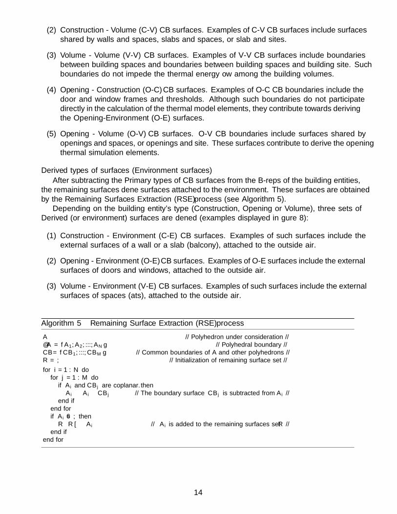
Derived types of surfaces (Environment surfaces)

After subtracting the Primary types of CB surfaces from the B-reps of the building entities,the remaining surfaces define surfaces attached to the environment. These surfaces are obtainedby the Remaining Surfaces Extraction (RSE) process (see Algorithm 5).

Depending on the building entity’s type (Construction, Opening or Volume), three sets ofDerived (or environment) surfaces are defined (examples displayed in figure 8):

(1) Construction - Environment (C-E) CB surfaces. Examples of such surfaces include theexternal surfaces of a wall or a slab (balcony), attached to the outside air.

(2) Opening - Environment (O-E) CB surfaces. Examples of O-E surfaces include the externalsurfaces of doors and windows, attached to the outside air.

(3) Volume - Environment (V-E) CB surfaces. Examples of such surfaces include the externalsurfaces of spaces (flats), attached to the outside air.

Algorithm 5 Remaining Surface Extraction (RSE) process

A // Polyhedron under consideration //∂A = {A1, A2, ..., AN} // Polyhedral boundary //CB = {CB1, ..., CBM} // Common boundaries of A and other polyhedrons //R = ∅ // Initialization of remaining surface set //

for i = 1 : N dofor j = 1 : M do

if Ai and CBj are coplanar. thenAi ← Ai − CBj // The boundary surface CBj is subtracted from Ai //

end ifend forif Ai 6= ∅ thenR ← R∪Ai // Ai is added to the remaining surfaces set R //

end ifend for

14

Wall

Wall

Slab

Wall – Wall(C – C) CB

Wall – Slab(C – C) CB

Space Wall

Wall – Space(C – V) CB

Site

Slab

Slab – Space(C – V) CB

Slab – Site(C – V) CB

Space Wall

Space – Space(V – V) CB

Space – Site(V – V) CB

Space

Wall

CONSTRUCTIONS (A1 – A2)

VOLUMES (A3)

A1. CONSTRUCTION - CONSTRUCTION

A2. CONSTRUCTION - VOLUME

A3. VOLUME - VOLUME

OPENINGS (A4 – A5)

Opening – Wall(O – C) CB

Opening – Slab(O – C) CB

Slab

Wall

Opening

A4. OPENING - CONSTRUCTION

Opening – Space(O – V) CB

Opening

A5. OPENING - VOLUME

Space

Slab

Wall – Space(C – V) CB

Wall

DerivedSpace

Environment(V – E) CB

Slab

Wall

Wall

Wall – Space(C – V) CB

Slab – Space(C – V) CB

Slab – Space(C – V) CB

Wall – Space(C – V) CB

Space

SLAB

Space

Wall – Slab(C – C) CB

Slab

Wall – Wall(C – C) CB

Wall – Slab(C – C) CB

Wall

Wall

Wall

Wall – Wall(C – C) CB

Wall – Space(C – V) CB

Derived Wall

Environment(C – E) CB

Opening – Space(O – V) CB

Wall

Opening Opening – Slab

(O – C) CB

Opening – Wall(O – C) CB

DerivedOpening

Environment(O – E) CB

Space

B2. VOLUME - ENVIRONMENT

B1. CONSTRUCTION - ENVIRONMENT

B3. OPENING - ENVIRONMENTSite

Slab

Figure 8: Primary types of common boundary surfaces referring to building constructions (A cases) and Derivedenvironment surfaces (B cases)

15

Common Boundary TypesC – V : Construction – VolumeC – E : Construction – EnvironmentV – V : Volume – VolumeO – V : Opening – VolumeO – E : Opening – Environment

CB : Common Boundary surface

RS : Remaining Surface

Space1

Space 2

Space3

CBI

Space1

Space2

Space3

C – V CB

C – V CB

O – V CB

C – E RS

C – E RS

C – V CB

V – V CB

O – E RS

PolyhedronA

PolyhedronB

Common Boundary(CB)

Figure 9: Geometrical illustration of CBI process on two polyhedrons (Top) – Plan view of the resulted CommonBoundaries (CB) for a three space building (Bottom)

Boundary Intersection Projection stage - BIP (stage 4)

The CB surfaces are forwarded to the Boundary Intersection Projection (BIP) process togenerate the required geometry elements (BIP elements) of a Building Energy Performance(BEP) simulation model. These elements, are essentially surface pairs, called CBIP surfaces orCBIPs. The BIP process can be described by two geometrical operations: (1) the projectionof one of the common boundaries on the plane of another; and (2) the intersection of theprojection with the other common boundary. In all cases, the surfaces of the generated BIPelements are related to a unique building entity (wall, slab, opening, etc.) and their normalvectors point away from this building entity.

The results of CBI and BIP operations for a simple example of three spaces’ floor plan, aredepicted in figures 9 and 10, respectively.

16

Common BoundaryIntersection & Projectionsurface types

(CBIP 1) & (CBIP 2) → (2a)

1. External Thermal Element(C – V) & (C – E) → (ETE)

2. Internal Thermal Element (C – V) & (C – V) → (ITE)

3. External Opening Element(C – V) & (O – E) → (EOE)

Common boundary (CB)

Projection

Intersection (CBIP)

Space1

Space2

Space3

BIP

C – V CBIP

C – V CBIP

C – E CBIP

C – V CBIP

C – E CBIP

V – V CBIP

O – V CBIP

O – E CBIP

Second level 2b space boundary extractionAfter all CBIP surface pairs and CB surfacesbeing subtracted from the B-rep of the buildingentity the remaining surfaces are 2b boundaries.

External Opening Element (EOE)(2a space boundary)Two CBIP surface pairs: one opening volume (O – V) andone opening environment (O – E).

External Thermal Element (ETE)(2a space boundary)Two CBIP surface pairs: one construction volume (C – V) andone construction environment (C – E).

Internal Air Element (IAE)(2a space boundary)One CBIP surface : Volume volume (V – V).

Internal Thermal Element (ITE)(2a space boundary)Two CBIP surface pairs: construction volume (C – V)

Common Boundary

A

CommonBoundary

B

CBIPB

CBIPA

Space1

Space2

Space3

C – V CB

C – V CB

O – V CB

C – E RS

C – E RS

C – V CB

V – V CB

O – E RS

Figure 10: Geometrical illustration of BIP process on two polyhedrons (Top) – Illustration of: C-V and O-V CBIP surface pairs, V-V Common Boundaries (CB) and extracted 2b space boundary surface types, for abuilding space (Bottom)

The projections of BIP process are applied to four types of CBs, derived from the CBI stage:C-V (Construction - Volume), C-E (Construction - Environment), O-V (Opening - Volume), O-E (Opening - Environment). In case a C-V, C-E, O-V or O-E common boundary is not projectedinto a C-V, C-E, O-V or O-E common boundary, it remains as a CB and is associated with aspecific building entity (wall, slab, opening, etc.). Such a case is depicted in figure 10 for a V-VCB surface of the examined space 1, which is also common boundary surface of space 2. Otherpossible CB surfaces not generating CBIP surface pairs are the common boundary surfaces ofthe C-C type.

Finally, a maximum distance criterion is used where a threshold value is used as an additionalparameter, in order to exclude the surface pairs, obtained from the BIP process, whose surfacesare far apart. Additionally, an outward normal criterion is used, where only the BIP elements,whose surface pairs have normal vectors pointing away from each other, are retained. As ageneral rule, the normal vector of a CB surface, the direction of which is preserved during theBIP process, always starts from the first element of the CB surface and points towards the

17

second element of the CB surface.

SlabSlab

A. Common Boundary Intersection B. Boundary Intersection projection

Air

: Distance of CB planes / BIP surfaces

: Maximum distance threshold

: Normal vector of : Common Boundaries / BIP Surfaces pointing away from construction

C – ECB

1

B2. IncludedBIP

Surface pairCB

1 – CB

5C – E CB2

C – E CB4

C – ECB

5

C – E CB3

B2. ExcludedBIP

Surface pairCB

2 – CB

3

B1. ExcludedBIP

Surface pairCB

3 – CB

4

Figure 11: Examples of three C-E CB surface pairs referring to a single building slab (A), generating three BIPelements (B). Two of the obtained BIP elements are excluded (one violating the maximum distance criterionand one violating the outward normal criterion) and one is included

An example where three C-E CB surface pairs related to a single building slab generate threeBIP elements, is displayed in figure 11. In this example, two of the obtained BIP elements obeythe maximum distance threshold criterion (figure 11 part B case B2). The remaining BIPelement violates the maximum distance criterion (figure 11, part B, case B1) and therefore isnot included. Additionally, out of the two BIP elements which obey the maximum distancecriterion, one BIP element is included since the normal vectors of its surfaces point away fromeach other (obeying the outward normal criterion), and one is excluded since the vectors of itssurfaces pointing towards each other.

Second-level boundaries of type 2a

After the completion of BIP process on all building elements of interest, the CBIP surfacepairs are obtained from the respective BIP elements. These CBIP surface pairs are related tothe 2nd-level space boundaries of type 2a (as defined in [5]), and are associated to the followingeight types of simulation model elements:

(1) External Thermal Elements (ETE).

External thermal elements are obtained by applying BIP on a Construction - Volume (C-V) / Construction - Environement (C-E) surface pair referring to the same constructionentity. A common example of such element is an external wall illustrated in case A offigure 12.

(2) Internal Thermal Elements (ITE).

Internal thermal elements are extracted using BIP on two Construction - Volume (C-V)CB surfaces, which refer to the same construction entity. Examples include internal wall’sspace boundary surfaces, as displayed in case B of figure 12 and slab - space boundarypairs.

18

(3) External Shading Elements (ESE). These elements are obtained by applying BIP on Con-struction - Environment (C-E) CB surfaces, which refer to the same construction entity(see figure 12 case C).

(4) Internal Shading Elements (ISE).

Internal Shading Elements refer to construction building entities which cause shadingeffects inside building spaces. They are obtained by applying the BIP process on twoConstruction - Volume (C-V) CB surfaces, referring to the same construction and volumeentities. Examples include recesses of building spaces caused by internal walls or slabs(see case D of figure 12).

(5) External opening elements (EOE).

External Opening Elements refer to surface pairs of building entities, that allow airflowbetween the environment and the building spaces. EOE are obtained by applying theBIP process on an Opening - Volume (O-V) CB surface and its Opening - Environment(O-E) CB surface counter part (see case E of figure 12).

(6) Internal Opening Element (IOE).

Similarly to the external opening elements, internal opening elements are representedby surface pairs of building entities, that allow airflow among building spaces. IOE areobtained using BIP on an Opening - Volume (O-V) CB surface pairs referring to the sameopening element (see case F figure 12).

(7) External Air Element (EAE).

External Air Elements are obtained directly from V-E CB surfaceswithout requiring BIP processing.

(8) Internal Air element (IAE).

Internal Air Elements are obtained directly from V-V CB surfaceswithout requiring BIP processing.

Second-level boundaries of type 2b and 2c

Apart from the second-level boundaries of type 2a, those of type 2b, 2c and 2d [5], are alsoextracted. These special cases of 2nd-level space boundaries can be ignored or be entered asadiabatic surfaces in a thermal simulation model. The extraction process of 2b, 2c and 2d spaceboundary types is similar to the RSE process, performed by Algorithm 5. Here, the polyhedronunder consideration A, is assigned to the B-rep of a building space, and not to a construction,

Additionally, the set CB, contains all the associated obtained CBIP surface pairs or CBsurfaces (C-V, O-V CBIPs or V-E, V-V CBs), related to this space (volume) which is representedby the polyhedron A. After executing a process similar to 5 the resulting set R, if its is notempty, will contain the second-level space boundaries of type 2b and 2c, associated with thespace volume under consideration.

An example of a 2b space boundary extraction, after all the CBIP and CB surfaces referringto a single space, are collected, is illustrated in the bottom part of figure 10.

19

Connectivity information

All of the previous types of elements are associated with certain connectivity informationwhich is also required in thermal simulations. CBIP provides this information in the form ofmatrices of different number of entries according to Table 1.

Table 1: Connectivity information of thermal elements.Ci. = Construction index, Isi = Internal space index, Ei = Environment index

Element Connectivity informationETE (Ci) / (Isi) / (Ei 1)ITE (Ci) / (1st Isi) / (2nd Isi)ESE n/aISE (Isi)EOE (Ci) / (Isi) / (Ei 1)IOE (Ci) / (1st Isi) / (2nd Isi)EAE (Isi) / (Ei 1)IAE (1st Isi) / (2nd Isi)

External and internal air elements have the same connectivity information with the respec-tive external and internal thermal and opening elements, without any construction associatedto them.

IFC data refinement

After the CBIP’s geometric operations, the IFC data can be updated using the results ofthe algorithm. More precisely, the surface pairs defined by the CBIP output elements describedearlier, can populate the IfcRelSpaceBoundary2ndLevel classes, as illustrated in the exampleof figure 13. The geometry of each boundary surface (surface polygon) is defined in the Con-nectionGeometry item. The boundary’s location, with respect to other building entities, isindicated by the InternalOrExternal item, which can potentially receive the following values:

• INTERNAL, if the boundary surface is attached to an internal building space (Boundaries#102, #103 and #105 in figure 13);

• EXTERNAL, if the boundary surface is attached to the outside air environment (Bound-aries #101, #104 and #106 in figure 13);

• EXTERNAL EARTH, if the boundary surface is attached to ground;

• EXTERNAL WATER, if the boundary surface is attached to water;

• EXTERNAL FIRE, if the boundary surface is attached to another building; and

• NOTDEFINED, if none of the previous cases holds.

1The environment index obtains two values: -1 if the environment entity refers to the building site and 0 ifthe environment entity refers to the outside air.

20

If the boundary surface refers to a building construction (wall, slab , etc.), the item Phys-icalOrVirtual receives the PHYSICAL value (boundaries #101, #102, #103, #104 in figure13); if it refers to a surface separating building spaces, the PhysicalOrVirtual receives the VIR-TUAL value (boundaries #105 and #106 in figure 13); otherwise, PhysicalOrVirtual becomesNOTDEFINED.

CBIP’s surface pairs are defined by the attribute CorrespondingBoundary. For example,the external wall of figure 13 contains a thermal element, defined by two boundary surfaces(#101, #102), which forms a pair indicated by the CorrespondingBoundary attribute (theCorresponding boundary of #101 is #102 and vice versa).

If a boundary surface contains openings (doors, windows, etc.), these openings are indicatedby the InnerBoundary attribute of the boundary surface, which contains the boundary surfacepairs of these openings. In figure 13 for example, the boundary surface #102 contains anopening indicated by the InnerBoundary #103. In the same manner, for the inner spaceboundaries, the space boundaries they belong to are indicated by the attribute ParentBoundary(as indicated in figure 13, inner boundaries #104 and #103 have boundaries #102 and #101as parent boundaries, respectively).

21

Space

Wall – Space(C – V) CB

Wall – Wall(C – C) CB

Wall – Slab(C – C) CB

Wall

ExternalWall

Wall – Wall(C – C) CB

Derived Wall

Environment(C – E) CB

Slab

Wall BIP

ExternalThermalElement(ETE)

Space

Slab

ExternalWall

DerivedSlab

Environment(C – E) CB

Space

Slab – Space(C – V) CB

Slab – Wall(C – C) CB

External Shading Element(ESH)

BIP

SlabOpening – Space

(O – V) CB

Opening Opening – Slab

(O – C) CB

Opening – Wall(O – C) CB

DerivedOpening

Environment(O – E) CB

BIP

ExternalOpeningElement(EOE)

Space

Wall – Space(C – V) CB

Wall – Wall(C – C) CB

Wall – Slab(C – C) CB

Wall

Internal Wall

Wall – Wall(C – C) CB

Slab

Wall BIP

InternalThermalElement

(ITE)

Wall – Space(C – V) CB

Wall

Space

Wall – Space(C – V) CB

Wall – Slab(C – C) CB

Wall – Wall(C – C) CB

Slab

Wall

BIP

Internal ShadingElement

(ISH)

Opening – Slab(O – C) CB

Wall

Opening

BIPSpace

InternalOpeningElement

(IOE)

Opening – Wall(O – C) CB

Opening – Space(O – V) CB

Space

A. EXTERNAL THERMAL ELEMENT (ETE)

C. EXTERNAL SHADING ELEMENT (ESE)

Wall

Space

E. EXTERNAL OPENING ELEMENT (EOE)

B. INTERNAL THERMAL ELEMENT (ITE)

D. INTERNAL SHADING ELEMENT (ISE)

F. INTERNAL OPENING ELEMENT (IOE)

Space

Wall

Slab

Opening – Space(O – V) CB

Figure 12: Simulation model element examples

.

If the boundary surface refers to an internal boundary attached to a specific building space,this space is indicated by the RelatingBuildingSpace attribute which points to the respectiveIfcSpace class. For instance, in figure 13, boundaries #102, #103 and #105 indicate space #1as their internal space.

Finally, the building element in which the boundary surface corresponds to, is indicated bythe RelatedBuildingElementattribute. If the boundary surface is a virtual boundary, such anattribute does not exist. In figure 13, the boundaries #101 #102 refer to an external wall andthe boundaries #103 and #104 refer to an external window.

Table 2 summarizes the relation between the surface pairs, obtained by CBIP, and theIFC space boundary surface types. For example, an external thermal element consists of twoPHYSICAL space boundary surfaces; the first is INTERNAL facing an internal building spaceand the second is EXTERNAL facing the outside air environment.

22

#1 SPACEOUTSIDE AIR

#101 IfcRelSpaceBoundary2ndLevel

- ConnectionGeometry = plane

- InternalOrExternalBoundary = EXTERNAL

- PhysicalOrVirtualBoundary = PHYSICAL

CorrespondingBoundary → #102

InnerBoundary → #104

RelatingBuildingSpace → #1 Space

RelatedBuildingElement → Wall

#104 IfcRelSpaceBoundary2ndLevel

- ConnectionGeometry = plane

- InternalOrExternalBoundary = EXTERNAL

- PhysicalOrVirtualBoundary = PHYSICAL

CorrespondingBoundary → #103

ParentBoundary → #101

RelatingBuildingSpace → #1 Space

RelatedBuildingElement → Window

#102 IfcRelSpaceBoundary2ndLevel

- ConnectionGeometry = plane

- InternalOrExternalBoundary = INTERNAL

- PhysicalOrVirtualBoundary = PHYSICAL

CorrespondingBoundary → #101

InnerBoundary → #103

RelatingBuildingSpace → #1 Space

RelatedBuildingElement → Wall

#103 IfcRelSpaceBoundary2ndLevel

- ConnectionGeometry = plane

- InternalOrExternalBoundary = INTERNAL

- PhysicalOrVirtualBoundary = PHYSICAL

CorrespondingBoundary → #104

ParentBoundary → #102

RelatingBuildingSpace → #1 Space

RelatedBuildingElement → Window

#105 IfcRelSpaceBoundary2ndLevel

- ConnectionGeometry = plane

- InternalOrExternalBoundary = INTERNAL

- PhysicalOrVirtualBoundary = VIRTUAL

CorrespondingBoundary → #106

RelatingBuildingSpace → #1 Space

#106 IfcRelSpaceBoundary2ndLevel

- ConnectionGeometry = plane

- InternalOrExternalBoundary = EXTERNAL

- PhysicalOrVirtualBoundary = VIRTUAL

CorrespondingBoundary → #105

RelatingBuildingSpace → #1 Space

ETE

ETE

ETE

ITE

ITE

EOE

EAE

Figure 13: Examples of IFC4 classes of second-level space boundaries and their related building entities andCBIP output elements

.

Table 2: CBIP output elements and respective IFC space boundary types.PHY = PHYSICAL, VIR. = VIRTUAL, INT = INTERNAL, EXT = EXTERNAL

Sim. Model 1st boundary 2nd boundaryElement surface surfaceETE PHY / INT PHY / EXTITE PHY / INT PHY / INTESE PHY / EXT PHY / EXTISE PHY / INT PHY / INTEOE PHY / INT PHY / EXTIOE PHY / INT PHY / INTEAE VIR / INT VIR / EXTIAE VIR / INT VIR / INT

Design requirements

In order to ensure the correct execution of CBIP algorithm certain design requirementsmust be satisfied, which are described in the following subsections.

23

Building site and spaces

The building entities which are associated with the operation of CBIP must contain at leastone element related to the building site and at least one element related to a building space.Such requirements are not met by the Design Transfer View 1.0 [33] model view definition.

The building site acts as a reference level in thermal simulations attaining the groundtemperature, which is considerably different than the air or building interior temperatures.Consequently, its presence and relative location to other building elements is of paramountimportance. On the other hand building spaces are associated with simulation output values(temperature, humidity, etc.) and therefore the presence and the geometrical definition of atleast one building space is prerequisite.

Curved solids

The geometric information of any curved building entity must be exported in the IFCfile considering a polyhedral approximation of the entity. This approximation must have itsboundary surfaces oriented according to the right hand outward normal rule, as explained inSection 2.1. Such a requirement can be set by the exporting software.

Design recommendations

Apart from the previous mandatory site and building space requirements, there are someadditional design recommendations, compliance of which guarantees accuracy of CBIP results.These recommendations are related to certain scenarios and are described in the followingsubsections.

Nonzero volume intersections

A nonzero volume intersection occurs when two or more building entities (wall, slab, space,etc) share a common nonzero volume, meaning that their solid geometric representations areintersected. Such cases can be identified using a model checking software such as Solibri [28].These cases do not impede the execution of CBIP, but affect the accuracy of its results. Theycan be corrected manually or automatically by using the algorithms of [27]. An example of anonzero volume intersection between a wall and a slab is displayed in the images of Case A1(inaccurate) and Case A2 (accurate) in figure 14.

Space-environment surfaces

The accuracy of CBIP results is also affected by the presence of space-environment surfacesassociated with internal surfaces. Space environment surfaces are derived surfaces of V-E type(see section 4.3.2), which define areas where a building space is not attached to any otherbuilding entity. These surfaces occur when an internal building space is not defined correctly,leaving small undefined space gaps between the space and surrounding building entities. Insuch cases the building spaces should be redefined correctly by redesign, or corrected using aspace correction algorithm [27]. Examples of space-environment surfaces related to an incorrectspace definition is displayed in the images of Case B1 (inaccurate) and Case B2 (accurate) offigure 14.

Curtain walls

If a curtain wall is present, it should always be contained inside an opening volume — avolume with surface area equal to the surface area of the curtain wall and thickness equal to thethickness of the wall it is attached to. This requirement is displayed graphically in the imagesof Case C1 (inaccurate) and Case C2 (accurate) of figure 14.

24

Suspended ceilings

If a suspended ceiling is present, the space volume beneath should extend to the floor (orthe roof if the space is in the last level) above it. This requirement is displayed graphicallyby the images of Case D1 (inaccurate) and Case D2 (accurate) of figure 14. Otherwise, anadditional space volume should be defined between the suspended ceiling and the floor, or roofabove it.

DESIGN RECOMMENDATIONS

Internal Building Space

Undesired Space Gap

Internal Building Space

Opening volume

Suspended ceiling

Internal BuildingSpace

Suspended ceiling

Case D2 (accurate)

After the space volume expansion the volume reaches the floor/roof of the level above.

Case C1 (inaccurate)

If no opening volume is defined in a curtain wall, an undesired space gap between the space volume and the plates/beams of the curtain wall exists.

Case C2 (accurate)

If the opening volume of a curtain wall is defined no undesired space gap exists.

Case D1 (inaccurate)

Space volume reachesthe bottom surface of the suspended ceiling

Internal BuildingSpace

SLAB

Case A1 (inaccurate)

A building slab intersects with a building wall. The volume of the intersection is nonzero.

Case A2 (accurate)

The building slab does not intersect with the adjacent wall. There is a common surface between the wall and slab.

SPACESPACE

Case B1 (inaccurate)

Space is incorrectly defined leaving undefined volume gaps indicated by the normal vectors

Case B2 (accurate)

Space is correctly definedWith no space-environment surfaces or undefined volume gaps.

IntersectionVolume

WALL

Clash SLAB

Figure 14: Design requirements for curtain walls (Left) and suspended ceilings (Right).

Orientation of boundary surfaces

To ensure accuracy in the results of CBIP, all of the involved building boundary represen-tations should be complete (without missing surfaces) and their boundary surface polygonsshould have a right-hand outward normal orientation, as described in Section 2.1. However,not all IFC exporting programs conform to such requirements. Therefore, an outward surfacenormal vector check of the involved polyhedrons and corrections were necessary, are required.

Comparison with other techniques

Several other techniques have been proposed for second-level space boundary generationwhich take as input the three dimensional geometry contained in IFC files and generate thesecond-level space boundary surface pairs using building graphs, as opposed to CBIP which isa graph-less method. In [22] graphs are constructed using the faces of building B-reps as graphvertexes and the connecting edges of the B-rep faces as graph edges. In [24] graphs are createdusing as vertexes the space construction common boundary surface and the construction partsbetween them and as edges the possible thermal flow paths. Finally in [23], graphs are used inorder to connect surface polygons of constructions (nodes) which ”view” one another using thedefinition and calculations of surface view factors.

All of the above methods do not require the geometrical definition of buildings’ conditionedspace air volumes and attempt to invoke such information based on the B-reps of the surround-ing constructions (walls, slabs, ...) and their connectivity. In this sense, these methods areparticularly useful in cases the conditioned building space volume data are missing. In such

25

cases CBIP cannot be applied, since it requires the geometrical definition of the conditionedbuilding space volumes. However, in the other methods there is no reference on the calculationof external shading surfaces (shading elements) and virtual space partitions (air elements), andsurfaces attached to building site (site boundaries). In this sense, CBIP can provide the spaceboundary surface pairs arising from virtual space partitioning, and building-site adjacency sinceit uses the geometrical definitions of the volumes of the spaces of the building and its site. Ad-ditionally CBIP can provide external shading surface computation which is useful for solar gaincalculation routines of building energy performance simulation programs.

Demonstration example

CBIP was applied successfully in several building reference cases including the ones describedin [34]. However, in order to include all possible geometrical complexities appearing in realbuildings, the algorithm is demonstrated here on the Technical Services building of TechnicalUniversity of Crete pictured in the upper part of figure 15. This building has two floors andfeatures highly complex geometry containing both convex and non-convex spaces.

A. Building B. Internal air elements

C. External thermal elements D. Internal thermal elements

E. Shading elements F. Opening elements

Figure 15: Demonstration building: Technical services building in Technical University of Crete (top-left) andresults of CBIP on the technical services building of the Technical University of Crete

.

As figure 15 demonstrates, CBIP correctly partitions the building walls and slabs according

26

to the topology of the building spaces. CBIP correctly identifies: the external and internalthermal elements (figure 15, parts C and D) the shading elements (figure 15, part E), the innerand outer opening elements (figure 15, part F), as well as the internal air elements (figure 15,part B) of this demonstration building. The total number of the identified elements as wellas their display colors are presented in Table 3. Based on these elements, the total identified2nd-level space boundary surfaces are 514, 122 of which are inner boundary surfaces referringto openings. During the BIP process, a maximum thickness threshold value of 1.2 meters, wasused.

Table 3: Simulation model elements of demonstration building (Total number / Display color)

Element No./color (wall) No./color (slabs)ETE 65 / white 14 / green - 15 / yellowITE 79 / white 13 / greenESE 18 / white 1 / greenISE 0 0EOE 41 / cyan 2 / yellowIOE 17 / blue 1 / redEAE 0 0IAE 10 / grey 0

Conclusions

It has been demonstrated that the proposed CBIP process generates the geometry of abuilding’s 2nd-level space boundaries, which are required for building energy simulations, basedon geometric information contained in IFC data files. In a nutshell, CBIP renders the processof energy simulation model generation, directly from IFC data semi-automatic. This fact,combined with the updatability and interoperability advantages of the IFC format, facilitatesthe data exchange between the BIM and energy simulation programs and enables a continuousbuilding performance monitoring.

In order to perform these operations CBIP uses the polyhedral geometric representations ofthe building entities. As its name reveals CBIP’s operation is based on two main subprocesses:the common boundary intersection (CBI) subprocess and the boundary intersection projection(BIP).

CBIP was applied on a highly complex building and the results demonstrated the abilityof the algorithm in handling non-convex geometries generating all the possible types of sim-ulation model elements including: thermal, opening, shading and air elements (virtual spaceboundaries). The second-level space boundaries were identified and their space connectivity in-formation was obtained accurately. In conclusion, CBIP automates the transformation processof IFC geometric data, to all the geometric data required for the creation of energy simulationmodels.

Acknowledgments

The research leading to these results has been partially funded by the European CommissionFP7-ICT-2011-6, ICT Systems for Energy Efficiency under contract #288409 (BaaS) and by theEuropean Commission H2020-EeB5-2015 project Optimised Energy Efficient Design Platformfor Refurbishment at District Level under contract #680676 (OptEEmAL).

27

[1] J. Clarke, Energy simulation in building design, Taylor & Francis, ISBN: 978-0-750-65082-3, 2012.

[2] K. Pratt, N. L. Jones, L. Schumann, D. Bosworth, A. Heumann, Automated translationof architectural models for energy simulation, in: Proc. of Symposium on Simulation forArchitecture and Urban Design, 6, Orlando,USA, 2012.

[3] G. Kontes, G. Giannakis, E. B. Kosmatopoulos, D. Rovas, Adaptive-fine tuning ofbuilding energy management systems using co-simulation, in: Proc. of IEEE In-ternational Conference on Control Applications, Zagreb, Croatia, 1664–1669, DOI:10.1109/CCA.2012.6402707, 2012.

[4] G. D. Kontes, C. Valmaseda, G. I. Giannakis, K. I. Katsigarakis, D. V. Rovas, In-telligent BEMS design using detailed thermal simulation models and surrogate-basedstochastic optimization, Journal of Process Control 24 (6) (2014) 846–855, DOI:10.1016/j.jprocont.2014.04.003.

[5] V. Bazjanac, Space boundary requirements for modeling of building geometry for energyand other performance simulation, in: Proc. CIB W78: 27th International Conference,Cairo, Egypt, 2010.

[6] C. Eastman, P. Teicholz, R. Sacks, K. Liston, BIM handbook: A guide to building infor-mation modeling for owners, managers, designers, engineers and contractors, Wiley, ISBN:978-0-470-54137-1, 2011.

[7] T. Liebich, IFC4-the new buildingSMART standard, in: IC meeting, bSI Publications,Helsinki, Finland, 2013.

[8] gbXML, The Green Building XML schema, <http://www.gbXML.org>, 2011.

[9] AutoDesk, RevitTM, <http://www.autodesk.com/products/autodesk-revit-family/overview>, 2014.

[10] GraphiSoft, ArchiCAD 17TM, <http://www.graphisoft.com/archicad/>, 2013.

[11] V. Bazjanac, Implementation of semi-automated energy performance simulation: buildinggeometry, in: CIB W, vol. 78, 2009.

[12] U.S. Dept. of Energy, EnergyPlus, <http://apps1.eere.energy.gov/buildings/energyplus/>, 2014.

[13] J. O’Donnell, T. Maile, C. Rose, N. Mrazovi, E. Morrissey, C. Regnier, K. Parrish, B. V.,Transforming BIM to BEM: Generation of Building Geometry for the NASA Ames Sus-tainability Base BIM, Tech. Rep., Simulation Research Group, 2013.

[14] M. Jokela, A. Keinanen, H. Lahtela, K. Lassila, O. Granlund, Integrated building simula-tion tool RIUSKA, in: Proc. of Building Simulation IBPSA conf., Prague, Czech Republic,1997.

[15] J. J. . A. Hirsch, DOE 2.1, <http://www.doe2.com>, 2014.

28

[16] A. Karola, H. Lahtela, R. Hanninen, R. Hitchcock, Q. Chen, S. Dajka, K. Hagstrom,BSPro COM-Server interoperability between software tools using industrial foundationclasses, Energy and Buildings 34 (9) (2002) 901–907, DOI: 10.1016/S0378-7788(02)00066-X.

[17] AutoDesk, Green Building StudioTM, <https://gbs.autodesk.com/GBS/>, 2014.

[18] T. Maile, M. Fischer, V. Bazjanac, Building energy performance simulation tools-a life-cycle and interoperable perspective, Center for Integrated Facility Engineering (CIFE)Working Paper 107 (2007) 1–49.

[19] TRNSYS, TRNSYS 17TM, <http://www.trnsys.com/>, 2014.

[20] IES, VE-proTM, <http://iesve.com/software/ve-pro>, 2014.

[21] R. Hitchcock, J. Wong, Transforming IFC Architectural View BIMs for Energy Simulation: 2011, in: Proc. of Building Simulation IBPSA conf., Sydney, Australia, 1089–1095, 2011.

[22] C. van Treeck, E. Rank, Dimensional reduction of 3D building models using graph theoryand its application in building energy simulation, Engineering with Computers 23 (2)(2007) 109–122, DOI: 10.1007/s00366-006-0053-7.

[23] N. L. Jones, C. J. McCrone, B. J. Walter, K. B. Pratt, D. P. Greenberg, Automatedtranslation and thermal zoning of digital building models for energy analysis, in: Proc. ofBuilding Simulation IBPSA conf., ISBN: 978-1-61839-790-4, 202–209, 2013.

[24] C. Rose, V. Bazjanac, An algorithm to generate space boundaries for building energysimulation, Engineering with Computers (2013) 1–10 .DOI: 10.1007/s00366-013-0347-5.

[25] G. N. Lilis, G. I. Giannakis, G. Kontes, D. V. Rovas, Semi-automatic thermal simulationmodel generation from IFC data, in: Proc. of European Conference on Product and ProcessModelling, Vienna, Austria, 503–510, DOI: 10.1201/b17396-83, 2014.

[26] G. N. Lilis, K. Sklivaniotis, G. Giannakis, D. Rovas, SRC: A systemic approach to buildingthermal simulation, in: Proc. of Building Simulation IBPSA conf., 3192–3199, 2013.

[27] G. N. Lilis, G. I. Giannakis, D. V. Rovas, Detection and semi-automatic correction of geo-metric inaccuracies in IFC files, in: Proc. of Building Simulation IBPSA conf., Hyderabad,India, 2182–2189, 2015.

[28] L. Khemlani, Solibri Model CheckerTM, CADENCE-AUSTIN (2002) 32–34.

[29] A. Borrmann, S. Schraufstetter, E. Rank, Implementing metric operators of a spatial querylanguage for 3D building models: octree and B-Rep approaches, Journal of Computing inCivil Engineering 23 (1) (2009) 34–46, DOI: 10.1061/(ASCE)0887-3801(2009)23:1(34).

[30] D. J. Jackson, Boundary representation modelling with local tolerances, in: Proc. ofthe third ACM symposium on Solid modeling and applications, ACM, 247–254, DOI:10.1145/218013.218067, 1995.

[31] W. Thibault, B. Naylor, Set operations on polyhedra using binary space partitioning trees,in: Proc. of the 14th annual conference on Computer graphics and interactive techniques,vol. 21, ACM, 153–162, DOI: 10.1145/37401.37421, 1987.

29

[32] B. Vatti, A generic solution to polygon clipping, Communications of the ACM 35 (7)(1992) 56–63, DOI: 10.1145/129902.129906.

[33] buildingSMART, Design Transfer View version 1.0, <http://www.buildingsmart-tech.org/mvd/IFC4Add1/DTV/1.0/html/>, 2015.

[34] M. Weise, T. Liebich, R. See, V. Bazjanac, T. Laine, B. Welle, Implementation guide:Space boundaries for energy analysis, General Services Administration (GSA) and OpenGeospatial Consortium (OSC) (2011) 1–62.

30

View publication statsView publication stats