Automatic differentiation applied to an inverse … EuroAd Workshop - Didier Auroux... ·...
27
Didier Auroux, Thomas Migliore Laboratoire J. A. Dieudonn´ e, Universit´ e de Nice Sophia Antipolis in collaboration with Laurent Hasco¨ et (INRIA), Jacques Blum (Univ. Nice), Laurent Loth and Daniel Coelho (ANDRA) Automatic differentiation applied to an inverse problem in geology Ninth Euro Automatic Differentiation Workshop, INRIA Sophia Antipolis. November 26-27, 2009
Transcript of Automatic differentiation applied to an inverse … EuroAd Workshop - Didier Auroux... ·...

Didier Auroux, Thomas Migliore
Laboratoire J. A. Dieudonne,
Universite de Nice Sophia Antipolis
in collaboration with Laurent Hascoet (INRIA), Jacques Blum (Univ. Nice), Laurent Loth
and Daniel Coelho (ANDRA)
Automatic differentiation applied to
an inverse problem in geology
Ninth Euro Automatic Differentiation Workshop,
INRIA Sophia Antipolis. November 26-27, 2009

Motivations
Nuclear waste storage : storage in deep level is considered by ANDRA
as the reference strategy for wastes with high or medium activity and long-lived.
Need for simulations of the radionucleide transport in underground impact
of a possible propagation of radioelements.
The modelling of the flow in porous media around the storage requires to
know the physical parameters of the different geological layers.
Those parameters (porosity and diffusion) are not directly accessible by mea-
surements, hence we have to solve an inverse problem to recover them.
9th Euro AD Workshop, INRIA, November 27 2009 1/26
Mathematical model
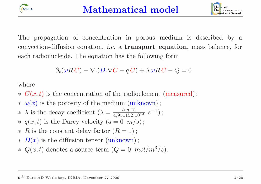
The propagation of concentration in porous medium is described by a
convection-diffusion equation, i.e. a transport equation, mass balance, for
each radionucleide. The equation has the following form
∂t(ωR C) −∇.(D.∇C − q C) + λ ωR C − Q = 0
where
∗ C(x, t) is the concentration of the radioelement (measured) ;
∗ ω(x) is the porosity of the medium (unknown) ;
∗ λ is the decay coefficient (λ = log(2)4,951152.1014 s−1) ;
∗ q(x, t) is the Darcy velocity (q = 0 m/s) ;
∗ R is the constant delay factor (R = 1) ;
∗ D(x) is the diffusion tensor (unknown) ;
∗ Q(x, t) denotes a source term (Q = 0 mol/m3/s).
9th Euro AD Workshop, INRIA, November 27 2009 2/26

Direct problem
We use the zonation method : the media is considered as a set of homogeneous
zones. The parameters are constant by zones : D = Di and ω = ωi in Ωi.
D =
10−11 m2/s on Ω1
10−6 m2/s on Ω2
10−10 m2/s on Ω3
ω =
0, 2 on Ω1
10 on Ω2
0, 3 on Ω3
C(t = 0) =
0 mol/m3 on Ω1 ∪ Ω3
1 mol/m3 on Ω2
D∇C(t, x).n = 0 on ∂Ω
9th Euro AD Workshop, INRIA, November 27 2009 3/26

Parameter estimation
Concentration values : the concentration is measured at final time on the
three lines γi, and on the subdomain Ω2 at every time.
Inverse problem : given Cobs, find porosity ω and diffusion D.
Cost function : quadratic misfit between the observations and the correspon-
ding quantities calculated by the model :
J(C(ω, D)) = α
∫ T
0
∫
Ω2
[
C − Cobs
]2dx dt + β
3∑
j=1
∫
γj
[
C(T ) − Cobs(T )]2
dx.
The weights α and β have been chosen to give comparable influence to the
two terms.
Goal : minimize J in order to find the optimal values of porosity and diffusion.
9th Euro AD Workshop, INRIA, November 27 2009 4/26

Twin experiments
Use of synthetic data :
• Choose values for the diffusion coefficient and the porosity ;
• Compute the resulting concentration Cobs in solving the forward problem ;
• Identify the diffusion and porosity from the observed concentration values.
Advantage : we can compare the porosity and the diffusion field calculated
by the inverse method to the initial porosity and diffusion field.
9th Euro AD Workshop, INRIA, November 27 2009 5/26

Minimization
We use gradient descent algorithms to minimize the criterion J we need to
compute the gradient of J with respect to ω and D.
The numerical gradient has been obtained by Automatic Differentation of the
direct code TRACES with the software TAPENADE developed by the Tropics
Team at INRIA Sophia-Antipolis generation of the adjoint code of TRACES.
We use the minimization software N2QN1 (quasi-Newton BFGS), which is a
bound constrained optimizer from Gilbert & Lemarechal (INRIA).
9th Euro AD Workshop, INRIA, November 27 2009 6/26
Automatic Differentiation
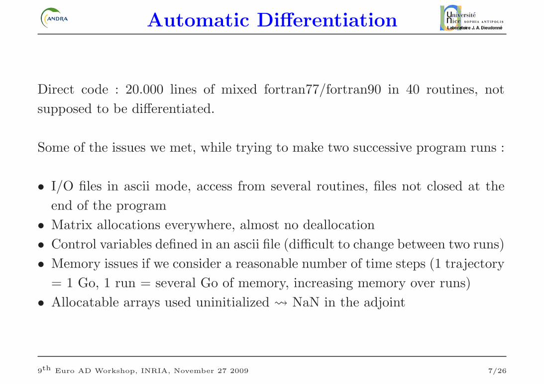
Direct code : 20.000 lines of mixed fortran77/fortran90 in 40 routines, not
supposed to be differentiated.
Some of the issues we met, while trying to make two successive program runs :
• I/O files in ascii mode, access from several routines, files not closed at the
end of the program
• Matrix allocations everywhere, almost no deallocation
• Control variables defined in an ascii file (difficult to change between two runs)
• Memory issues if we consider a reasonable number of time steps (1 trajectory
= 1 Go, 1 run = several Go of memory, increasing memory over runs)
• Allocatable arrays used uninitialized NaN in the adjoint
9th Euro AD Workshop, INRIA, November 27 2009 7/26

Automatic Differentiation
Main modifications :
• Store the trajectory (for generating the observations in twin eperiments)
• Define the cost function
• Change I/O ASCII files to binary files (with direct access)
• Rewrite initialization, allocations, deallocations, ...
• Rewrite the main time loop routine (do call onetimestep enddo)
• Remove the prints to standard output
and then play again with Tapenade !
9th Euro AD Workshop, INRIA, November 27 2009 8/26
Automatic Differentiation
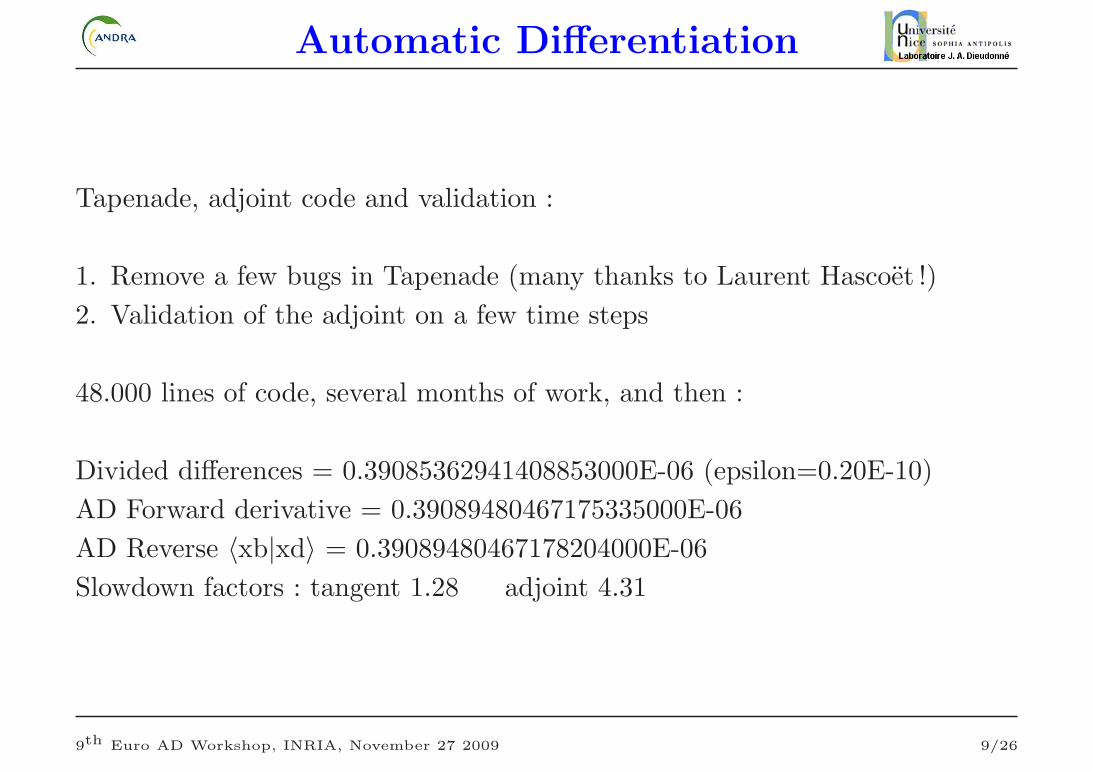
Tapenade, adjoint code and validation :
1. Remove a few bugs in Tapenade (many thanks to Laurent Hascoet !)
2. Validation of the adjoint on a few time steps
48.000 lines of code, several months of work, and then :
Divided differences = 0.39085362941408853000E-06 (epsilon=0.20E-10)
AD Forward derivative = 0.39089480467175335000E-06
AD Reverse 〈xb|xd〉 = 0.39089480467178204000E-06
Slowdown factors : tangent 1.28 adjoint 4.31
9th Euro AD Workshop, INRIA, November 27 2009 9/26

Gradient validation
3. Validation of the adjoint with finite differences on a few time steps
r(ε) =J(K + ε δK) − J(K)
ε 〈∇J(K), δK〉−→ε→0
1
9th Euro AD Workshop, INRIA, November 27 2009 10/26

Gradient validation
4. and then validation on the “full” program
Diffusion parameters : 9.6E-7 0.00021 Porosity parameters : 0.0011 0.32
Cost function : f = 2.0258486318199945E-8
Adjoint gradient : g = -0.0018222876539832878 0.00008205308963214484
0.000001979478809560615 1.418571652819071E-7
Finite diff gradient : g = -0.0018222227804698817 0.00008205309952898589
0.00000197947976722247 1.418515488854936E-7
Slowdown factors : tangent 1.41 adjoint 5.44
Max Stack size : 10199 blocks of 16384 bytes => total :159.359375 Mbytes
C Traffic : 4945 Mb and 305450 millionths
F Traffic : 62 Mb and 73256 millionths
Divided differences = 0.30208125371924738381E-05 (epsilon=0.20E-10)
AD Forward derivative = 0.30210378956057821803E-05
AD Reverse <xb|xd> = 0.30210378956057436403E-05
Various evolutions of the code, modification of the location/number of obser-
vations, modification of the number of control variables, . . .
9th Euro AD Workshop, INRIA, November 27 2009 11/26
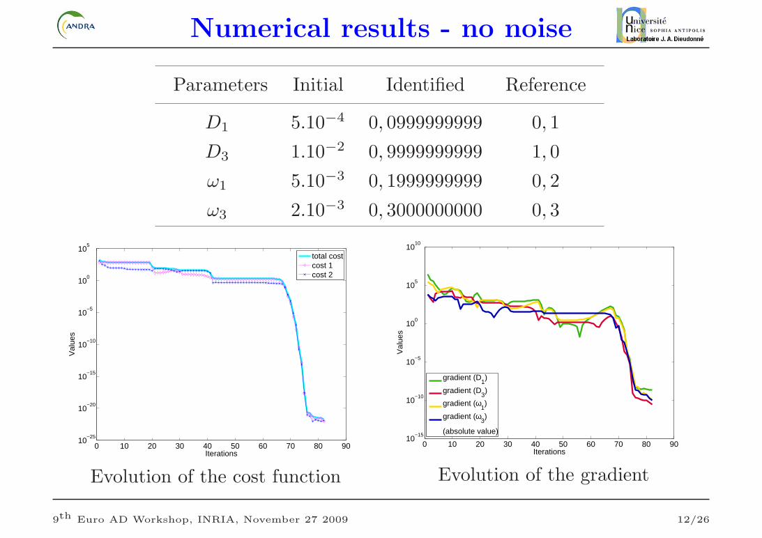
Numerical results - no noise
Parameters Initial Identified Reference
D1 5.10−4 0, 0999999999 0, 1
D3 1.10−2 0, 9999999999 1, 0
ω1 5.10−3 0, 1999999999 0, 2
ω3 2.10−3 0, 3000000000 0, 3
0 10 20 30 40 50 60 70 80 9010
−25
10−20
10−15
10−10
10−5
100
105
Iterations
Val
ues
total costcost 1cost 2
Evolution of the cost function
0 10 20 30 40 50 60 70 80 9010
−15
10−10
10−5
100
105
1010
Iterations
Val
ues
gradient (D1)
gradient (D3)
gradient (ω1)
gradient (ω3)
(absolute value)
Evolution of the gradient
9th Euro AD Workshop, INRIA, November 27 2009 12/26
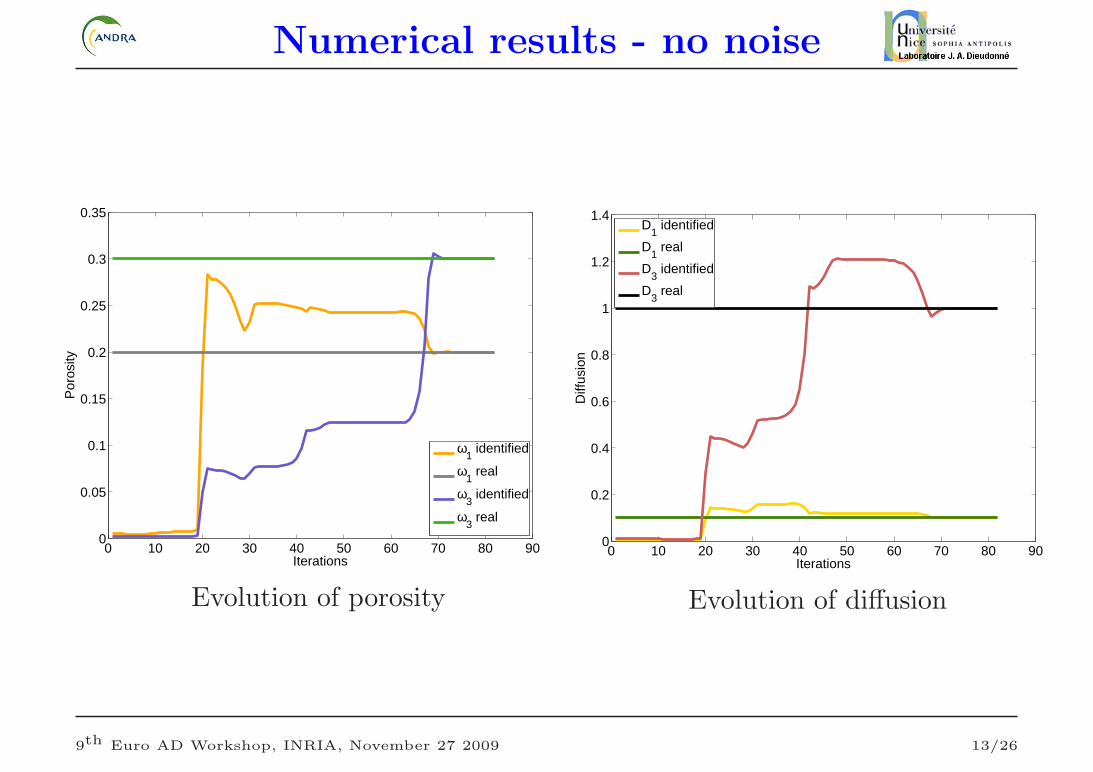
Numerical results - no noise
0 10 20 30 40 50 60 70 80 900
0.05
0.1
0.15
0.2
0.25
0.3
0.35
Iterations
Por
osity
ω1 identified
ω1 real
ω3 identified
ω3 real
Evolution of porosity
0 10 20 30 40 50 60 70 80 900
0.2
0.4
0.6
0.8
1
1.2
1.4
IterationsD
iffus
ion
D1 identified
D1 real
D3 identified
D3 real
Evolution of diffusion
9th Euro AD Workshop, INRIA, November 27 2009 13/26

Numerical results - noisy data
5% noise
on the data
Parameters Initial Identified Reference
D1 5.10−4 0, 1018767983 0, 1
D3 1.10−2 0, 9552432582 1, 0
ω1 5.10−3 0, 2049359853 0, 2
ω3 2.10−3 0, 1729395267 0, 3
0 10 20 30 40 50 60 70 80 9010
−2
10−1
100
101
102
103
104
Iterations
Val
ues
total costcost 1cost 2
Evolution of the cost function
0 10 20 30 40 50 60 70 80 9010
−10
10−5
100
105
1010
Iterations
Val
ues
gradient (D1)
gradient (D3)
gradient (ω1)
gradient (ω3)
(absolute value)
Evolution of the gradient
9th Euro AD Workshop, INRIA, November 27 2009 14/26

Numerical results - noisy data
0 10 20 30 40 50 60 70 80 900
0.05
0.1
0.15
0.2
0.25
0.3
0.35
Iterations
Por
osity
ω1 identified
ω1 real
ω3 identified
ω3 real
Evolution of porosity
0 10 20 30 40 50 60 70 80 900
0.2
0.4
0.6
0.8
1
1.2
1.4
IterationsD
iffus
ion
D1 identified
D1 real
D3 identified
D3 real
Evolution of diffusion
9th Euro AD Workshop, INRIA, November 27 2009 15/26
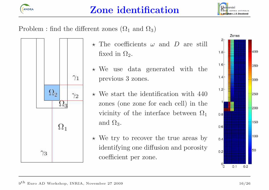
Zone identification
Problem : find the different zones (Ω1 and Ω3)
⋆ The coefficients ω and D are still
fixed in Ω2.
⋆ We use data generated with the
previous 3 zones.
⋆ We start the identification with 440
zones (one zone for each cell) in the
vicinity of the interface between Ω1
and Ω3.
⋆ We try to recover the true areas by
identifying one diffusion and porosity
coefficient per zone.
9th Euro AD Workshop, INRIA, November 27 2009 16/26

Numerical results - N zones
Diffusion at
iteration 1
Diffusion at
iteration 947
True
diffusion
9th Euro AD Workshop, INRIA, November 27 2009 17/26

Numerical results - N zones
Porosity at
iteration 1
Porosity at
iteration 947
True
porosity
9th Euro AD Workshop, INRIA, November 27 2009 18/26
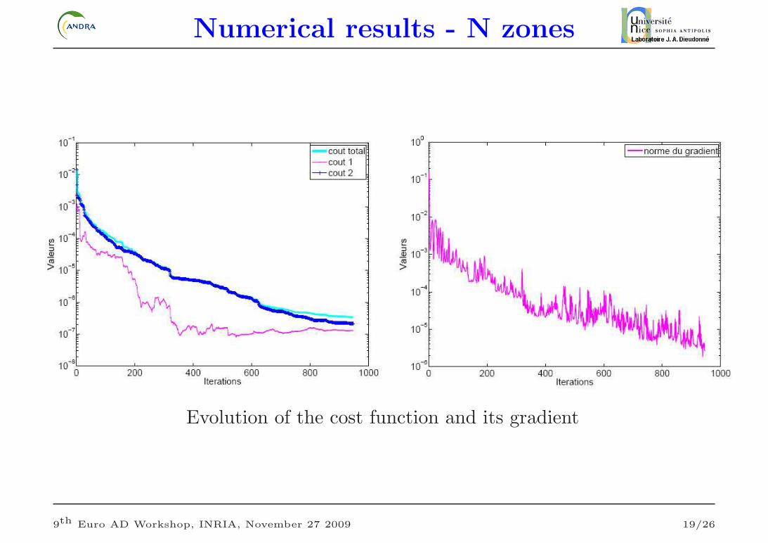
Numerical results - N zones
Evolution of the cost function and its gradient
9th Euro AD Workshop, INRIA, November 27 2009 19/26

Zone identification
⋆ We need to regularize the inverse
problem.
⋆ We add some a priori physical infor-
mation : the domain has a revolution
symmetry five concentric zones.
⋆ We start the identification with these
7 zones (five + Ω1 + Ω2) where the
coefficients are constant.
⋆ We try to recover the true areas by
identifying one diffusion and porosity
coefficient by zone.
9th Euro AD Workshop, INRIA, November 27 2009 20/26

Numerical results - no noise
True porosity
Porosite − iteration1
0
0.05
0.1
0.15
0.2
0.25
Porosity at iteration 1 Porosity at iteration 179
9th Euro AD Workshop, INRIA, November 27 2009 21/26

Numerical results - no noise
True diffusion Diffusion at iteration 1 Diffusion at iteration 179
9th Euro AD Workshop, INRIA, November 27 2009 22/26
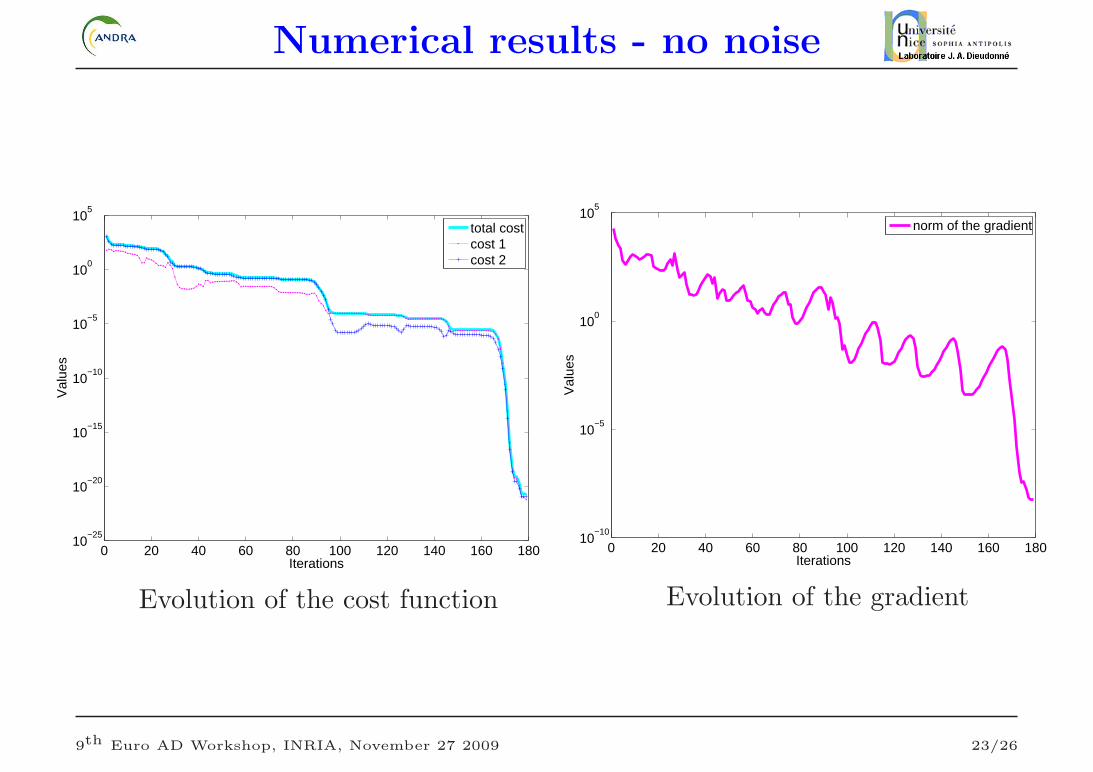
Numerical results - no noise
0 20 40 60 80 100 120 140 160 18010
−25
10−20
10−15
10−10
10−5
100
105
Iterations
Val
ues
total costcost 1cost 2
Evolution of the cost function
0 20 40 60 80 100 120 140 160 18010
−10
10−5
100
105
IterationsV
alue
s
norm of the gradient
Evolution of the gradient
9th Euro AD Workshop, INRIA, November 27 2009 23/26
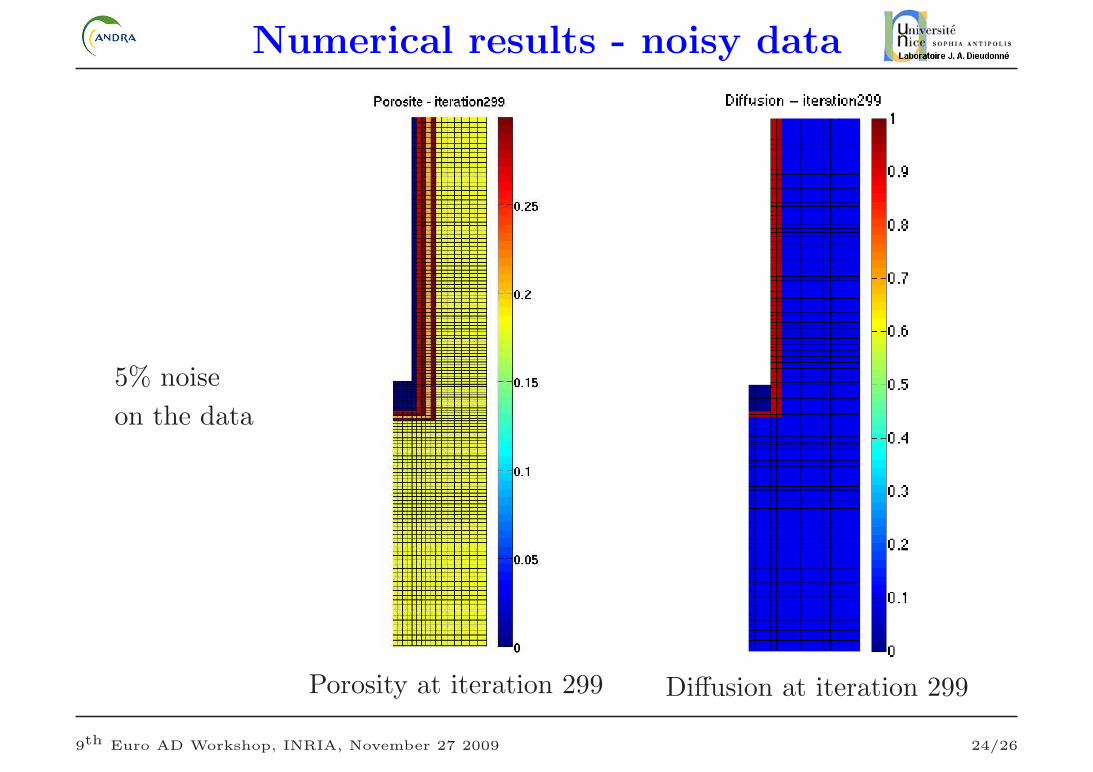
Numerical results - noisy data
5% noise
on the data
Porosity at iteration 299 Diffusion at iteration 299
9th Euro AD Workshop, INRIA, November 27 2009 24/26

Numerical results - noisy data
0 50 100 150 200 250 30010
−2
10−1
100
101
102
103
Iterations
Val
ues
total costcost 1cost 2
Evolution of the cost function
0 50 100 150 200 250 30010
−4
10−2
100
102
104
106
IterationsV
alue
s
norm of the gradient
Evolution of the gradient
9th Euro AD Workshop, INRIA, November 27 2009 25/26

Conclusions
• We now have the adjoint code of TRACES, thanks to TAPENADE
• The parameter estimation works in 2D
• The adjoint and optimization techniques have been validated with a large
number of zones
• The zone identification problem can be solved by using concentric zones
∗ Sensitivity studies (small sensitivity to the porosity in Ω3 ?)
∗ 3D code (2D axisymmetric)
∗ Compare with other methods (topological optimization, refinement indica-
tors, . . .)
9th Euro AD Workshop, INRIA, November 27 2009 26/26