Automatic Detection and Segmentation of Brain …...Automatic Detection and Segmentation of Brain...
96
Automatic Detection and Segmentation of Brain Lesions from 3D MR and CT Images By Molise Mokhomo A Dissertation submitted to the Faculty of Engineering in fulfillment of the requirement for the degree of Master of Science at the University of Cape Town Supervisors: A/Prof. F. Nicolls (UCT), Prof. G. de Jager (UCT) and Dr. N. Muller (iThemba LABS) University of Cape Town May 26, 2014
Transcript of Automatic Detection and Segmentation of Brain …...Automatic Detection and Segmentation of Brain...
Automatic Detection and Segmentation ofBrain Lesions from 3D MR and CT Images
ByMolise Mokhomo
A Dissertation submitted to the Faculty of Engineeringin fulfillment of the requirement for the degree
of Master of Scienceat the
University of Cape Town
Supervisors: A/Prof. F. Nicolls (UCT), Prof. G. de Jager (UCT) andDr. N. Muller (iThemba LABS)
University of Cape Town
May 26, 2014

Declaration
I declare that this dissertation is my own work. All the resources that I have used have been
referenced and listed in the Bibliography. It is being submitted for the degree of Master of Science
in Engineering at the University of Cape Town and has not been submitted before for any degree
or examination at any other university.
I know the meaning of plagiarism and declare that all the work in the document, save for that which
is properly acknowledged, is my own.
Signed:__________________________________
Date:____________________________________
Molise Mokhomo
i

Acknowledgments
I would like to thank the following people
• My supervisor at UCT, Dr. F. Nicolls, for his guidance and motivating me to do this work.
Without him this work could have taken months off my life.
• My UCT Co-supervisor, Prof. G. de Jager, for his support and encouragement.
• My supervisor at iThemba LABS, Dr. N. Muller, for his help and encouragement.
• iThemba LABS for the financial support.
• My family for their love and support.
ii
Abstract
The detection and segmentation of brain pathologies in medical images is a vital step which helps
radiologists to diagnose a variety of brain abnormalities and set up a suitable treatment. A number
of institutes such as iThemba LABS still rely on a manual identification of abnormalities. A manual
identification is labour intensive and tedious due to the large amount of medical data to be processed
and the presence of small lesions. This thesis discusses the possible methods that can be used to
address the problem of brain abnormality segmentation in MR and CT images. The methods are
general enough to segment different types of abnormalities. The first method is based on the
symmetry of the brain while the second method is based on a brain atlas.
The symmetry-based method assumes that healthy brain tissues are symmetrical in nature while
abnormal tissues are asymmetric with respect to the symmetry plane dividing the brain into simi-
lar hemispheres. The three major steps involved in this approach are the symmetry detection, tilt
correction and asymmetry quantification. The method used to determine the brain symmetry au-
tomatically is discussed and its accuracy has been validated against the ground-truth using mean
angular error (MAE) and distance error (DE). Two asymmetric quantification methods are studied
and validated on real and simulated patient’s T1- and T2-weighted MR images with low and high-
grade gliomas using true positive volume fraction (TPVF), false positive volume fraction (FPVF)
and false negative volume fraction (FNVF).
The atlas-based method is also presented and relies on the assumption that abnormal brain tissues
appear with intensity values different from those of the surrounding healthy tissues. To detect and
segment brain lesions the test image is aligned onto the atlas space and voxel by voxel analysis
is performed between the atlas and the registered image. This methods is also evaluated on the
simulated T1-weighted patient dataset with simulated low and high grade gliomas. The atlas,
containing prior knowledge of normal brain tissues, is built from a set of healthy subjects.
iii

Contents
Declaration i
Acknowledgements ii
Abstract iii
Abbreviations xiv
Symbols and Notations xv
1 Introduction 1
1.1 Problem Statement . . . . . . . . . . . . . . . . . . . . . . . . . . . . . . . . . . 2
1.2 Objectives of the Study . . . . . . . . . . . . . . . . . . . . . . . . . . . . . . . . 2
1.3 Contributions . . . . . . . . . . . . . . . . . . . . . . . . . . . . . . . . . . . . . 3
1.4 Organization of this Document . . . . . . . . . . . . . . . . . . . . . . . . . . . . 3
2 Brain tumor and Computer Aided Diagnosis Methods 4
2.1 Brain tumors . . . . . . . . . . . . . . . . . . . . . . . . . . . . . . . . . . . . . 4
2.1.1 Diagnosis and Treatment of Brain Tumors . . . . . . . . . . . . . . . . . 5
2.2 Computer Aided Diagnosis (CAD) in Brain Pathologies . . . . . . . . . . . . . . . 6
2.2.1 Knowledge-Based Brain Tumor Detection Techniques . . . . . . . . . . . 6
2.2.2 Supervised Brain Tumor Detection Methods . . . . . . . . . . . . . . . . 7
2.2.3 Unsupervised Brain Tumor Detection Methods . . . . . . . . . . . . . . . 7
2.2.4 Atlas Based Methods . . . . . . . . . . . . . . . . . . . . . . . . . . . . . 8
2.2.4.1 Research in Brain Atlas Construction . . . . . . . . . . . . . . . 8
iv

Contents v
2.2.4.2 Delineating Brain Tumors Using a Brain Atlas . . . . . . . . . . 9
2.2.5 Symmetry Quantification Methods . . . . . . . . . . . . . . . . . . . . . . 10
2.2.5.1 Research in Brain Symmetry Plane Estimation . . . . . . . . . . 10
2.2.5.2 Delineation of Brain Tumors Using Asymmetry Analysis . . . . 11
2.3 Conclusion . . . . . . . . . . . . . . . . . . . . . . . . . . . . . . . . . . . . . . 12
3 Medical Image Registration 13
3.1 Feature Spaces . . . . . . . . . . . . . . . . . . . . . . . . . . . . . . . . . . . . 14
3.2 Transformation model . . . . . . . . . . . . . . . . . . . . . . . . . . . . . . . . 14
3.2.1 Rigid Transformation . . . . . . . . . . . . . . . . . . . . . . . . . . . . 14
3.2.2 Affine Transformation . . . . . . . . . . . . . . . . . . . . . . . . . . . . 15
3.2.3 Nonrigid Transformation . . . . . . . . . . . . . . . . . . . . . . . . . . 16
3.3 Similarity Measure . . . . . . . . . . . . . . . . . . . . . . . . . . . . . . . . . . 16
3.3.1 Sum of Square Difference (SSD) . . . . . . . . . . . . . . . . . . . . . . . 16
3.3.2 Absolute Difference (AD) . . . . . . . . . . . . . . . . . . . . . . . . . . 17
3.3.3 Correlation Coefficient (CC) . . . . . . . . . . . . . . . . . . . . . . . . . 17
3.3.4 Mutual Information (MI) . . . . . . . . . . . . . . . . . . . . . . . . . . . 17
3.4 Optimization Methods . . . . . . . . . . . . . . . . . . . . . . . . . . . . . . . . 19
3.4.1 Gradient Descent (GD) Method . . . . . . . . . . . . . . . . . . . . . . . 20
3.4.2 Newton’s Method . . . . . . . . . . . . . . . . . . . . . . . . . . . . . . . 20
3.4.3 Quasi-Newton (QN) Method . . . . . . . . . . . . . . . . . . . . . . . . 21
3.4.4 Gauss-Newton (GN) Method . . . . . . . . . . . . . . . . . . . . . . . . 21
3.4.5 Levenberg-Marquardt Method (LM) . . . . . . . . . . . . . . . . . . . . . 22
3.5 Techniques to Improve Optimization Methods . . . . . . . . . . . . . . . . . . . . 23
3.5.1 Multi-Resolution Approach . . . . . . . . . . . . . . . . . . . . . . . . . 23
3.5.2 Sampling Strategies . . . . . . . . . . . . . . . . . . . . . . . . . . . . . 23
3.6 Conclusion . . . . . . . . . . . . . . . . . . . . . . . . . . . . . . . . . . . . . . 23
4 Overview of the Symmetry and Atlas-Based Methods 25
4.1 Motivation for Choosing Knowledge-Driven Methods . . . . . . . . . . . . . . . . 26

Contents vi
4.2 Assumptions . . . . . . . . . . . . . . . . . . . . . . . . . . . . . . . . . . . . . 28
4.3 Outline of the Proposed Methods . . . . . . . . . . . . . . . . . . . . . . . . . . . 28
4.3.1 Anomaly Detection Using Symmetry Analysis Method . . . . . . . . . . . 28
4.3.2 Anomaly Detection Using an Atlas . . . . . . . . . . . . . . . . . . . . . 30
4.3.2.1 Atlas Construction . . . . . . . . . . . . . . . . . . . . . . . . . 30
4.3.2.2 Detecting Anomalies . . . . . . . . . . . . . . . . . . . . . . . 31
4.4 Conclusion . . . . . . . . . . . . . . . . . . . . . . . . . . . . . . . . . . . . . . 31
5 Symmetry Plane Detection and Asymmetry Quantification in CT and MR Images 32
5.1 Symmetry Axis in 2D Images . . . . . . . . . . . . . . . . . . . . . . . . . . . . . 33
5.1.1 Symmetry Detection . . . . . . . . . . . . . . . . . . . . . . . . . . . . . 33
5.1.2 Symmetry Detection Results . . . . . . . . . . . . . . . . . . . . . . . . . 34
5.2 Mid-Sagittal Plane Detection . . . . . . . . . . . . . . . . . . . . . . . . . . . . . 34
5.2.1 Geometry of the MSP . . . . . . . . . . . . . . . . . . . . . . . . . . . . 34
5.2.2 Isotropic Resampling . . . . . . . . . . . . . . . . . . . . . . . . . . . . . 36
5.2.3 Feature Space . . . . . . . . . . . . . . . . . . . . . . . . . . . . . . . . . 37
5.2.4 3D Reflection Transformation Matrix . . . . . . . . . . . . . . . . . . . . 37
5.2.5 Similarity Measure . . . . . . . . . . . . . . . . . . . . . . . . . . . . . . 38
5.2.6 Optimization Using Levenberg-Marquardt (LM) Method . . . . . . . . . . 38
5.2.7 Multi-Resolution . . . . . . . . . . . . . . . . . . . . . . . . . . . . . . . 40
5.3 Tilt Correction . . . . . . . . . . . . . . . . . . . . . . . . . . . . . . . . . . . . . 41
5.4 Asymmetry Quantification Using Registration . . . . . . . . . . . . . . . . . . . . 42
5.4.1 Nonrigid Registration . . . . . . . . . . . . . . . . . . . . . . . . . . . . . 43
5.4.2 Detection of Abnormal Region by Thresholding Image Difference . . . . . 43
5.4.3 Removing False Positives . . . . . . . . . . . . . . . . . . . . . . . . . . 44
5.4.4 Detect the Ill Hemisphere Using Feature Factors . . . . . . . . . . . . . . 44
5.4.4.1 Uncover Ill Hemisphere Using Prior Knowledge . . . . . . . . . 45
5.4.4.2 Uncover Ill Hemisphere Without a Priori Knowledge . . . . . . 45
5.5 Asymmetry Quantification Using Maximally Stable Extrema Region Detection . . 46
5.5.1 Literature on Region Detection . . . . . . . . . . . . . . . . . . . . . . . . 47

Contents vii
5.5.2 Detection of Interest Region . . . . . . . . . . . . . . . . . . . . . . . . . 47
5.5.3 Removing False Positives . . . . . . . . . . . . . . . . . . . . . . . . . . 48
5.6 Results and Discussion . . . . . . . . . . . . . . . . . . . . . . . . . . . . . . . . 48
5.6.1 Dataset Used . . . . . . . . . . . . . . . . . . . . . . . . . . . . . . . . . 48
5.6.2 Determining Accuracy Measure . . . . . . . . . . . . . . . . . . . . . . . 49
5.6.3 Determining Parameter Values . . . . . . . . . . . . . . . . . . . . . . . . 50
5.6.4 Results . . . . . . . . . . . . . . . . . . . . . . . . . . . . . . . . . . . . 52
5.6.4.1 Evaluation of the MSP . . . . . . . . . . . . . . . . . . . . . . . 52
5.6.4.2 Evaluation of Registration and Region Detection Asymmetry
Analysis Method . . . . . . . . . . . . . . . . . . . . . . . . . . 54
5.6.4.3 Summary . . . . . . . . . . . . . . . . . . . . . . . . . . . . . . 57
6 Atlas-Based Pathology Detection 60
6.1 Building Atlas . . . . . . . . . . . . . . . . . . . . . . . . . . . . . . . . . . . . . 60
6.1.1 Generalized Procrustes Analysis (GPA) . . . . . . . . . . . . . . . . . . . 60
6.1.1.1 Choosing Initial Reference . . . . . . . . . . . . . . . . . . . . 61
6.1.1.2 Image Alignment . . . . . . . . . . . . . . . . . . . . . . . . . 61
6.1.1.3 Procrustes Distance (PD) . . . . . . . . . . . . . . . . . . . . . 63
6.1.2 Atlas Construction . . . . . . . . . . . . . . . . . . . . . . . . . . . . . . 63
6.2 Abnormal Tissue Detection . . . . . . . . . . . . . . . . . . . . . . . . . . . . . . 64
6.2.1 Abnormality Detection on Full Scans . . . . . . . . . . . . . . . . . . . . 64
6.2.2 Abnormality Detection on Partial Scans . . . . . . . . . . . . . . . . . . . 66
6.3 Removing False Positives . . . . . . . . . . . . . . . . . . . . . . . . . . . . . . . 68
6.4 Results and Discussion . . . . . . . . . . . . . . . . . . . . . . . . . . . . . . . . 68
6.4.1 Evaluation on Full Scan . . . . . . . . . . . . . . . . . . . . . . . . . . . 69
6.4.2 Summary . . . . . . . . . . . . . . . . . . . . . . . . . . . . . . . . . . . 71
7 Conclusion 72
7.1 Summary of this Thesis . . . . . . . . . . . . . . . . . . . . . . . . . . . . . . . . 72
7.2 Limitations and Future Work . . . . . . . . . . . . . . . . . . . . . . . . . . . . . 73

Contents viii
Bibliography 74
List of Figures
2.1 Illustration of the appearance of brain tumors on MRI. From left to right: axial slice of
patient diagnosed with low-grade glioma, patient diagnosed with meningiomas, patient
diagnosed with astrocytoma. Dataset is from [1]. . . . . . . . . . . . . . . . . . . . . . 5
2.2 The appearance of healthy brain tissues on CT and MR images: (first row) axial, coronal
and sagittal slice CT scan, (second row) axial, coronal and sagittal slices from MR scan.
The CT data is from iThemba LABS and MR is taken from [2]. . . . . . . . . . . . . . 6
3.1 Image registration using multi-resolution. Adapted from [3]. . . . . . . . . . . . . . . . 24
4.1 Simulated axial slices showing symmetric and asymmetric brain abnormalities (red) with
the symmetry axis (white line) superimposed on each slice. From left to right: asymmet-
ric lesion (red) lying on the left hemisphere, two symmetric lesions (red) placed on both
hemispheres and a large lesion crossing the symmetry axis. . . . . . . . . . . . . . . . . 27
4.2 Simulated axial slices showing symmetric and asymmetric brain abnormalities (green) hav-
ing overlapping intensity with healthy tissues. The symmetry axis (white line) is superim-
posed on each slice. From left to right: asymmetric lesion (green) lying on the left hemi-
sphere, two symmetric lesions placed on both hemispheres and a large lesion crossing the
symmetry axis. . . . . . . . . . . . . . . . . . . . . . . . . . . . . . . . . . . . . . 27
4.3 Illustration of the atlas sample. . . . . . . . . . . . . . . . . . . . . . . . . . . . . . 27
4.4 General workflow of the symmetry analysis method. . . . . . . . . . . . . . . . . . . . 29
5.1 Symmetry detection results on 2D images. The symmetry line (green) is overlaid on MR
(first row), CT (second row) and simulated binary images (third row). In the right-bottom
image, the algorithm converged to the global minimum of the cost function and there is no
clear symmetry in this image due to the shearing of the left half of the object. . . . . . . . 35
5.2 From left to right: 3D view of a full scan head, illustration of the MSP (black) passing
through the head. . . . . . . . . . . . . . . . . . . . . . . . . . . . . . . . . . . . . 36
ix

List of Figures x
5.3 Results for CT and MRI scan after tilt correction: (first row) misaligned scans with the
MSP overlaid on each slice; (second row) corresponding slices after tilt correction. . . . . 42
5.4 Results for image difference before and after applying nonrigid registration. From left to
right: (1) axial slice from left hemisphere, (2) right hemisphere before registration, (3) reg-
istered right hemisphere, (4) intensity difference before registration, (5) intensity difference
after registration, (6) suspected lesions regions for λ = .8 and ζ = .001, (7) lesion regions
overlaid on intensity difference. The parameters λ and ζ define the maximum intensity
difference ratio and threshold between feature vectors respectively and are discussed later
in Section 5.6.3. . . . . . . . . . . . . . . . . . . . . . . . . . . . . . . . . . . . . 43
5.5 Estimated artificial lesion’s longest diameter (LD): (a) Welded left-hand and right-hand
hemispheres after performing nonrigid registration, (b) Highly asymmetric regions for λ =
.8 andζ = .001, (c) Asymmetric regions (red contour) and LD (green line) for each region
superimposed on axial slice, (d) Asymmetric regions with LD≥ 10 mm. . . . . . . . . . 44
5.6 Suspected lesions locations on both hemispheres. From left to right: the regions (green)
surrounding lesion regions (red) superimposed on the left hemisphere,the regions (green)
surrounding lesion regions (red) superimposed on the right hemispheres, most asymmetric
regions (red) on the left hemisphere, most asymmetric regions (red) on the right hemisphere. 46
5.7 Results for MSRE region detection. From left to right: input axial slice from the left
hemisphere, input axial slice from the right hemisphere, highly asymmetric stable regions
detected on the left hemisphere, highly asymmetric stable regions detected on the right
hemisphere for ζ = 0.001. . . . . . . . . . . . . . . . . . . . . . . . . . . . . . . . 48
5.8 Dataset used to validate lesion asymmetry analysis method. First column shows a healthy
CT scan. Second and third columns depict T1- and T2-weighted MR scans respectively
of a single patient with high-grade gliomas. The last column shows the MR image of a
patient with high-grade meningiomas. . . . . . . . . . . . . . . . . . . . . . . . . . . 49
5.9 The effect of varying parameters on a healthy subject. First row: Left, and reflected right
hemisphere and the absolute difference between the hemispheres. Second row: Detected
false positives superimposed on left and right hemisphere as parameter λ is varied. λ is
set to 0.5 in the first two columns and to 0.7 in the last two columns. Third row: welded
left, and right hemispheres after an ill hemisphere is determined for ζ = 0.1 and λ = 0.5.
In the second and third image ζ = 0.1 and ζ = 0.2 respectively for λ = 0.7. It is noticed
that increasing the value of ζ reduces the number of false positives. . . . . . . . . . . . . 51
5.10 Top left, top right, bottom left and bottom right quadrants show the subject with artificial
lesion of radius 30, 40, 50 and 60 mm respectively. In each quadrant first and second
column (first row before tilt correction, second row after tilt correction) show the MSP
projected and overlaid on the axial and coronal slices. The third column depicts a 3D view
of the MSP cutting through the head. . . . . . . . . . . . . . . . . . . . . . . . . . . 53
List of Figures xi
5.11 Results for a volume subjected to rotation transformation. Top left, top right, bottom left
and bottom right quadrants shows the subject rotated by 20o about x-, y-, z- and xyz-axes
respectively. In each quadrant first column shows the MSP projected on the axial slice
before and after tilt correction. The second column shows the MSP projected and overlaid
on the coronal slices. The third column depicts 3D view of the MSP cutting through the
head. . . . . . . . . . . . . . . . . . . . . . . . . . . . . . . . . . . . . . . . . . . 55
5.12 Results shown on axial slices for patients (first column to third column) and simulated
dataset (fourth to seventh column) with high-grade gliomas. First row shows the raw input
data while the second and the third row depicts the results obtained using the registration
and region detection methods respectively. . . . . . . . . . . . . . . . . . . . . . . . . 56
5.13 Results depicted on axial slices for patients (first column to fourth column) and simulated
dataset (fifth to seventh column) with low-grade gliomas. First row shows the raw input
data while the second and the third row depicts the results obtained using the registration
and region detection methods respectively. . . . . . . . . . . . . . . . . . . . . . . . . 58
6.1 Brain atlas in T1-weighted MR images acts as the model of healthy brain tissues. From top
to bottom: axial, coronal and sagittal view of the atlas. From left to right: expected grey
level, maximum intensity variance, expected norm of the displacement field, and maximum
variance norm of the displacement field for each voxel. . . . . . . . . . . . . . . . . . . 65
6.2 Intermediate results for atlas-based tumor detection method. Top row from left to right:
mean intensity (MI), maximum intensity variance (MV ), test image before registration (F),
deformed test image after registration (F̄), the intensity square difference (DI) between (VI)
and (F̄), binary image where (DI > VI). Bottom row from left to right: mean displacement
field (MV ), maximum variance of the displacement field (VV ), the deformation field norm
(U) of the registered test image, displacement field square difference (DV ) between (MV )
and (U), binary image where (DV > VV ). The binary images mark the suspected location
of the anomalies. . . . . . . . . . . . . . . . . . . . . . . . . . . . . . . . . . . . . 67
6.3 Illustration of removing false positives using binary images where voxels (with white in-
tensity color) have unexpected intensity distribution or deformation field. From left to
right: (a) deformed input image, and voxels with: (b) unexpected grey level values, (c)
large deformation field, (d) unexpected grey level values and large deformation field. The
rightmost binary image marks the final suspected location of the lesions. . . . . . . . . . 68
6.4 The results for atlas-based method depicted on axial slice for simulated dataset with high-
grade gliomas. First row: raw input data, second row: deformed test image with suspected
location (red contour) overlaid on each image. . . . . . . . . . . . . . . . . . . . . . . 69

List of Figures xii
6.5 The results for atlas-based method depicted on axial slice for simulated dataset with low-
grade gliomas. First row: raw input data, second row: deformed test image with the
estimated location (red contour) of the lesions superimposed on each image. . . . . . . . 70

List of Tables
5.1 Tolerance to pathological asymmetries. . . . . . . . . . . . . . . . . . . . . . . . . . 52
5.2 Tolerance to rotation. . . . . . . . . . . . . . . . . . . . . . . . . . . . . . . . . . . 54
5.3 Accuracy results for patient and simulated dataset with high-grade gliomas. . . . . . . . 57
5.4 Quantitative results for patient and simulated dataset with low-grade gliomas. . . . . . . 57
6.1 Accuracy results for atlas-based method applied on simulated T1-weighted dataset with
high-grade gliomas. . . . . . . . . . . . . . . . . . . . . . . . . . . . . . . . . . . 70
6.2 Quantitative results for atlas-based method applied on simulated T1-weighted dataset with
low-grade gliomas. . . . . . . . . . . . . . . . . . . . . . . . . . . . . . . . . . . . 70
xiii

Abbreviations
CAD Computer Aided Diagnosis
CT Computed Tomography
DE Distance Error
FLAIR Fluid-Attenuated Inversion Recovery
FNVF False Negative Volume Fraction
FPVF False Positive Volume Fraction
GPA Generalized Procrustes Analysis
LM Levenberg-Marquardt
MAE Mean Angular Error
MI Mutual Information
MRI Magnetic Resonance Imaging
MSER Maximally Stable Extrema Region
MSP Mid-Sagittal Plane
NMI Normalized Mutual Information
RECIST Response Evaluation Criteria in Solid Tumors
SSD Sum of Square Difference
TPVF Truth Positive Volume Fraction
xiv

Symbols and Notations
R Reference image
F Floating image
Ti 3D affine transformation
TRF 3D reflection matrix
MI Mean intensity volume of the atlas
MV Mean displacement field norm
VI Intensity variations for each voxel
VV Displacement field variations for each voxel
p Vector point in 3D
u Optimization parameter
µ Damping factor
λ Maximum intensity difference ratio
ζ Threshold
xv
Chapter 1
Introduction
Medical imaging is a routine and essential part of medicine where computerized applications are
used to assist clinicians and radiologists to carry out daily activities within healthcare. A number
of applications include computer aided pathology diagnosis, computer aided image registration,
planning and guiding treatment, and monitoring disease progression based on the information ex-
tracted from medical images. The major advantage of this field is that health problems can be
observed directly rather than derived from the symptoms. Health problems can, for example, be
broken bones, brain abnormalities, breast, and prostate cancer. In this work much attention is put
on computer aided brain lesions diagnosis.
A brain lesion is a localized abnormal structural change of the brain tissues. Various factors that
lead to brain lesion development include brain injuries, vascular disorders and brain tumors. Brain
lesions are often a threat to life hence their diagnosis and treatment is of great importance to patients
suffering from them. Nowadays, different imaging modalities are used to acquire medical images
for visualization of internal human body structures such as tissues of the brain and neck. The
most common imaging technologies used are computed tomography (CT) and magnetic resonance
imaging (MRI). The advantage that MRI has over CT is that it is harmless, since it does not use
ionization radiation, and produces high quality images with soft tissue contrast that is much better
than that with CT [4]. Moreover, MRI can distinguish tissues that have similar intensities and are
hard to distinguish using CT scans.
Automatic detection and segmentation of brain abnormalities from CT or MR images is a chal-
lenging task since lesions can appear at any location and have different intensity distributions.
However, having prior knowledge about healthy tissues of the brain can simplify this task. The
prior knowledge about the symmetry of healthy brain tissues can be used to detect a number of
brain pathologies. Additionally it can also be the grey level distribution of healthy tissues which
can be presented in the form of the brain atlas. The brain atlas is built from single image or a set of
specific population images aligned onto a common coordinate frame through image registration.
1
1.1. Problem Statement 2
Image registration is the process of bringing two images of the same or different patients taken
at the different times into a common coordinate frame such that the images can be compared,
combined or analyzed voxel by voxel. The registration technique can either be global or local.
Global registration methods apply a single transformation to the entire image to correct rotation,
translation, scaling and shearing between the two images. Local registration techniques apply
different transformations on each voxel to correct shape differences.
The accurate delineation of brain abnormalities is of great importance for setting a suitable treat-
ment for a patient diagnosed with brain tumors. In this thesis, symmetry and atlas-based methods
for automated brain anomaly segmentation are developed and applied to a large dataset of brain
T1- and T2-weighted MR images.
1.1 Problem Statement
Hand labeling of brain pathologies in medical images is often regarded as the gold-standard tech-
nique to segment brain abnormalities. This method is currently used at iThemba LABS by a ra-
diologist to monitor the response of the brain tumors before and after the treatment. However,
this approach becomes tedious in the presence of small sized brain lesions and time consuming
due to the large amount of data to be analyzed or the presence of multiple tumors having different
sizes. Moreover, the results are usually operator-dependent. Therefore developing an automated
computer aided brain pathology diagnostic application can save radiologists time in setting up a
suitable treatment for a patient diagnosed with brain tumors.
Numerous automated methods for segmenting brain pathologies have been developed. These meth-
ods vary depending on the characteristics of the tumors to be segmented and the type of image
modality used [5]. The lesion attributes which have made automated segmentation a challenging
task include the variety of shapes and sizes the lesions may possess. Additionally they have a
likelihood of appearing at any location and with different intensity distributions. Because of these
factors, there is no general brain lesions segmentation method which can be adopted widely in
every application.
1.2 Objectives of the Study
Implementing a fast and efficient computer aided diagnosis (CAD) technique for brain pathologies
is quite useful. Hence this work seeks to solve the mentioned challenges by developing a model of
healthy brain tissues. The model will be used to assist radiologists at iThemba LABS to identify
the presence of brain lesions in medical images and to monitor the deviation of the lesions from
previous and future CT and MR images before and after the patient is treated. The other objective is
to evaluate the accuracy of the implemented methods against the ground truth. This will determine

1.3. Contributions 3
how well the methods perform under varying condition.
1.3 Contributions
Two knowledge-driven methods have been developed to detect and segment a large number of low
and high-grade brain tumors in 3D MR images. They utilize prior knowledge of healthy brain
tissues to address a variety of brain pathologies. The prior information used include the symmetry
of the brain and expected grey level distribution of healthy brain tissues.
Firstly using the knowledge about the symmetry of a healthy brain, two novel methods have been
developed for the quantification of brain asymmetry level to determine brain pathologies. One
of the techniques analyzes the intensity difference between the left and right hemispheres to esti-
mate the location of brain pathologies in the two hemispheres. Given the suspected tumor regions,
the method further analyzes the intensities of the voxels surrounding these regions to find the ill
hemisphere. The other approach uses a region of interest detection method to determine hemi-
spheres with asymmetric tissues which often represent brain tumors. An algorithm that detects the
symmetry plane in healthy and abnormal 3D brain scans was also implemented.
Secondly an atlas-based method, which uses prior information about healthy anatomical structures
of the brain, is developed to address the mentioned problems. This algorithm is automatic and
segments different brain anomalies in test images having a modality similar to those of the images
used to build the atlas. An improved atlas construction method is also proposed. The atlas consists
of the information similar to the work presented in [6].
1.4 Organization of this Document
The remaining parts of this document are organized as follows. Chapter 2 presents the background
knowledge of the brain tumor characteristics and covers the literature of the different computer
aided diagnostic methods used to detect and segment brain lesions. Chapter 3 describes global
medical image registration with much attention paid to 3D image datasets. In Chapter 4, the pro-
posed two methods used to detect and segment brain anomalies are presented. The first approach
is based on the symmetry of a healthy human brain while the second technique is founded on a
model of healthy brain tissues. The implementation and testing of brain symmetry detection and
analysis methods are given in Chapter 5. Chapter 6 describes the implementation and results of the
atlas-based method. Finally, Chapter 7 concludes the thesis and gives suggestions for future work
and for some improvements.

Chapter 2
Brain tumor and Computer AidedDiagnosis Methods
A solid background knowledge about the characteristics of brain tumors is useful for researchers
to implement computerized applications used to detect and segment tumors in medical images.
This chapter discusses different criteria and characteristics used to classify some of the commonly
known brain tumors and their appearance in medical images in Section 2.1. It further gives an
overview of some of the techniques proposed in the literature used to assist radiologists to estimate
the location of brain pathologies in medical images in Section 2.2. The conclusion is provided in
Section 2.3.
2.1 Brain tumors
This thesis focuses on methods used to detect and segment brain tumors. A brain tumor is an
abnormal new mass of tissue arising from brain cells and brain structures. It can be classified as
either a primary or a secondary brain tumor [7, 8]. A tumor is said to be primary if it is the major
cause of the cancer in the brain and secondary if it is caused by the spread of cancer from other
body organs, for example breast or lung cancer spreading to the brain.
Primary brain tumors containing no cancer cells are called benign while those that contains cancer
cells are called malignant. The cells of the benign tumor rarely invade healthy tissues around them.
Malignant brain tumors are likely to grow rapidly and invade neighboring brain tissues hence are
often a threat to life [7]. The malignancy of the tumor is determined based on its location, growth
rate and historical features.
Primary brain tumors are normally classified based on the tissue of origin. The most common
type of tumors are called gliomas which originate from glial cells. They can be described as
low-grade (slow growing) or high-grade (very aggressive) [7]. Different types of gliomas include:
4

2.1. Brain tumors 5
(1) astrocytoma which originate from astrocytes and glioblastoma multiforme which is a form of
high-grade astrocytoma, (2) oligodendroglioma which develops from oligodendrocytes. Another
common type of brain tumors is called meningioma and arises from meninges surrounding the
brain and spinal cord.
The cause of brain tumors is still an unanswered question and studies have been made to find out
whether people with certain risk factors are likely to develop a brain tumor. The results found a
major environmental risk factor is exposure to ionizing radiation [7]. Moreover there are major
concerns that heredity could be one of the causes of brain cancer. Figure 2.1 shows the appearance
of a number of brain tumors in T2-weighted MR images for patients diagnosed with a low-grade
glioma, meningioma and astrocytoma. The tumors differ in shape, location and have different
appearances. In the first and the third image, the tumors appear having lower intensity values than
those of the surrounding healthy tissues. The middle image shows a meningioma located on the
left frontal lobe having intensity values larger than those of the white matter surrounding it.
Figure 2.1: Illustration of the appearance of brain tumors on MRI. From left to right: axial slice of patientdiagnosed with low-grade glioma, patient diagnosed with meningiomas, patient diagnosed with astrocytoma.Dataset is from [1].
2.1.1 Diagnosis and Treatment of Brain Tumors
Imaging modalities are used to diagnose different brain tumors and then treatment follows. The
two common imaging techniques used are MRI and CT. MRI uses magnetic fields, electromagnetic
radiation and a computer to reconstruct images of the brain while CT uses X-rays and a computer
to reconstruct brain images [4]. MRI gives good contrast between different soft tissues while CT
provides a better contrast between bone and soft tissues. In addition, MRI is said to be harmless
to patients compared to CT as it does not use ionizing radiation as the external source of energy.
When a patient is diagnosed with a brain tumor a specific treatment is suggested based on a number
of factors such as the type, size and location of the tumor, age and general health of the patient. The
treatment options for people with brain tumors are surgery, radiation therapy, and chemotherapy. A
combination of treatments can also be suggested. Figure 2.2 shows the appearance of the healthy
brain from two different patients on CT and MR images.

2.2. Computer Aided Diagnosis (CAD) in Brain Pathologies 6
Figure 2.2: The appearance of healthy brain tissues on CT and MR images: (first row) axial, coronal andsagittal slice CT scan, (second row) axial, coronal and sagittal slices from MR scan. The CT data is fromiThemba LABS and MR is taken from [2].
2.2 Computer Aided Diagnosis (CAD) in Brain Pathologies
Computer aided diagnosis is the concept of using a computerized application to process and manip-
ulate multidimensional medical images of anatomical structures of patients to visualize the diag-
nostic features [9]. It is used in applications such as detection and segmentation of brain anatomical
structures, breast and brain cancers tissues and other body organs in MR and CT images. Addition-
ally it is used to register images of the same or different patients acquired at different times. The
major role that CAD has brought to the field of medicine is the increase of the diagnostic accuracy
as the radiologist uses results from the application as a second opinion to make final decisions [9].
It also reduces the processing time hence giving the doctors a chance to decide the best treatment
for the diagnosed disease on time. However, automatic identification and segmentation of diag-
nosed brain structures is still a challenging problem due to the variability of protocols used during
scanning and orientation from patient to patient.
This section discusses different methods proposed in the literature used to detect and segment brain
pathologies in medical images. It also discusses the techniques used to detect the symmetry plane
and atlas construction of the brain.
2.2.1 Knowledge-Based Brain Tumor Detection Techniques
Knowledge-based brain tumor methods use the information extracted from a knowledge source to
detect brain tumors from medical images. The knowledge base is built using anatomical features of
the tumor of interest such as expected size, grey level pixel color, shape and neighborhood relation-
2.2. Computer Aided Diagnosis (CAD) in Brain Pathologies 7
ships with other brain tissues. The knowledge is then encoded into rules which can be inferred or
is transformed into a geographical template with tissue labels assigned [10]. The advantage these
methods have is that less training data is required. Their major drawback is that they are static
in nature and hence are likely to fail to model a variety of brain tumors since tumor’s anatomical
properties vary from patient to patient [10, 11].
2.2.2 Supervised Brain Tumor Detection Methods
Supervised brain tumor detection methods rely on the use of manually annotated training data.
These methods develop the model from the training data set and uses the same model to recognize
new test data at a later stage. The major disadvantage of these methods is that they are labour
intensive and time consuming. Also they are likely to fail to perform well if there is an overlap of
intensity distributions between healthy and abnormal brain tissues.
A number of supervised methods have been proposed and used to detect and segment brain tumors
from CT and MR images. In [12] Patil and Udupi propose a probabilistic neural network to classify
brain tumors. Their technique consists of four main stages which include preprocessing, segmen-
tation, feature extraction and classification. Cherifi et al. [13] implemented a classification method
based on expectation maximization segmentation. Their method is automatic and works for both
tissue recognition and tumor extraction. Jafari and Kasaei in [14] present a neural network-based
method for automatic classification of brain MR images. Their method classifies tissues into three
categories: normal, tumor benign and malignant. They use the discrete wavelet transform (DWT)
to obtain features related to each MRI and applied principal component analysis to reduce feature
dimensions to obtain more meaningful features. After the essential features have been extracted,
a supervised feed-forward back-propagation neural network technique is used to classify the sub-
jects. Khalid et al. [15] use k-nearest neighbor to segment abnormalities from brain MR images.
They perform preliminary data analysis to extract feature vectors of the brain structures and use
minimum, maximum and mean grey level pixel values as their feature vectors components. In other
research Abdullah [5] introduces a new method used to segment multiple sclerosis (MS) lesions
from brain MRI data. The technique uses textural features to detect MS lesions in a fully automatic
approach. A trained support vector machine (SVM) is used to classify regions of MS lesions and
non-MS lesions.
2.2.3 Unsupervised Brain Tumor Detection Methods
Unsupervised methods also need training data but the data need not to be annotated. Instead the
training data is annotated using clustering algorithms which make unsupervised method less labor
intensive when compared to supervised methods [16, 17]. The elements in each cluster are related
to each other in some way. For example, they may be closer, in terms of distance, to a particular
point than to other elements in a different cluster. Like supervised methods they also fail to perform

2.2. Computer Aided Diagnosis (CAD) in Brain Pathologies 8
well if there is an overlap of intensity distributions between healthy and abnormal brain tissues.
This normally occurs if they rely on bad features such as intensity alone. Hence the appropriate
choice of the features has to be taken into consideration.
In [13] Cherifi et al provide a comparison between two image segmentation methods. One of the
methods is based on segmentation using thresholding techniques and the other method is based
on expectation maximization (EM) segmentation. They use these techniques to detect, segment,
classify and measure properties of normal and abnormal brain tissues. From their analysis they
find that EM gives better results when compared to thresholding especially when detecting small
regions. Anitha et al. in [18] design a method used to automatically identify the white matter
lesions found in the brains of elderly people. The method starts by preprocessing input images
and then follows by clustering using fuzzy c-means (FCM), geostatistical possibilistic clustering
(GPC) and lastly geostatistical fuzzy clustering (GFCM). They conclude that GFCM detects the
large region of lesions and gives a smaller false positive rate when compared to FCM and GPC.
2.2.4 Atlas Based Methods
A brain atlas is the average brain image of an individual or multiple individuals in a specific age
or race group [9]. It contains the knowledge base of brain structures in the form of intensity or
probability distribution and is used to register different images onto the same coordinate space to
allow subsequent comparison of brain structures and functions across individuals [19]. To construct
an atlas from a group of individual images, one of the images is selected as the reference image.
The remaining images are registered to the reference image and then an average image is computed
from the aligned images. The difficulty faced by atlas-based methods is variability of brain size
and shape across groups of people [9, 19]. Hence researchers often prefer to build a population
based brain atlas.
2.2.4.1 Research in Brain Atlas Construction
Various algorithms have been developed to construct brain atlases. An atlas is constructed over a
defined coordinated space onto which all images must be aligned. One of the most used coordinate
spaces is the Talairach atlas [20]. It applies a piecewise affine transform to 12 rectangular regions
of the brain to register new images in defined spaces [19]. It became a gold-standard used to
align images for functional activation sites in positron emission tomography (PET) and functional
magnetic resonance imaging (fMRI) studies [19, 21, 22]. Though it was adopted as the gold-
standard the Talairach atlas still has a number of limitations. Firstly the brain used by Talairach
and Tournoux was smaller in size compared to average brain size [21, 22, 23]. Secondly the atlas
was created based on single subject (postmortem brain) of a 60-year old French woman hence
it does not provide anatomy of all living subjects. Lastly the slice gap and thickness, and the
inconsistency of the orthogonal plane sections, have presumably limited the use of their work in

2.2. Computer Aided Diagnosis (CAD) in Brain Pathologies 9
recent studies [21, 22, 23].
Ortega et al. [24] construct a deformable brain atlas and used it to identify subthalamic nucleus
in T1-weighted MRI. Firstly an MRI dataset is transformed into the Talairach coordinate system
manually. Secondly segmentation of homologous structures both in the atlas and MRI image of
the patient’s brain follows, and lastly non-rigid registration is applied between the segmented struc-
tures.
In order to address limitations of the Talairach atlas, the Montreal Neurological Institute (MNI) cre-
ated a population-specific brain atlas, MNI-305 [21, 22]. This template was generated by manually
registering 250 images of 305 brain MRI right-handed images onto the Talairach brain atlas and
the aligned images were averaged to construct the MNI-250 brain atlas. The remaining 55 images
were automatically registered onto MNI-250 using a linear transform. The manually registered 250
images and the 55 linearly registered images were averaged to form the MNI-305 brain atlas. Spe-
cific medical groups around the world adopted MNI templates as their standard [21]. They build
brain atlases after aligning their data set onto MNI space. Despite the dominant use of MNI space
and the fact that it is population specific some researchers have proposed novel techniques, though
still population dependent, to construct their atlases. For example, a Korean brain template and
a French brain template were constructed and used to represent the brain characteristics of Asian
and French populations respectively [22, 23, 25, 26]. Tang et al. [22] develop a new brain atlas
to facilitate computational brain studies in Chinese populations using MRI. Their template is also
population specific for Chinese people. They use 3.0 Tesla MRI scans of 56 right-handed Chinese
males. In [21] Mandal et al. summarize the history, construction and application of brain atlases.
Their study focuses on brain atlases starting from the Talairach atlas to a Chinese brain atlas. They
also provide a new automated work-flow protocol they use to design a population-specific brain
atlas from MRI data.
2.2.4.2 Delineating Brain Tumors Using a Brain Atlas
Several methods have been proposed to encode the knowledge base of healthy brain tissue in
the form of a brain atlas. These methods have given radiologists across the globe a chance to
understand functional activities of the brain. They are also helpful to diagnose and detect different
pathologies arising from brain tissues [6, 27, 28, 29]. Prastawa et al. [29] describe an automated
brain tumor segmentation framework from MR images; both T1-weighted and T2-weighted images
are used. Their proposed method detects abnormal tissues using a registered brain atlas as a model
of a healthy brain. They use T2 image densities to determine whether there is an edema in the
abnormal region, and then apply geometric and spatial constraints to separate the edema and the
tumor. In another research report, Bourouis and Hamrouni [27] present a novel deformable model
for 3D tumor segmentation based on a level-set concept. They use both boundary and regional
information to define the speed function. Their method is automatic and applicable to T1-weighted
pre-contrast and post contrast 3D images.
2.2. Computer Aided Diagnosis (CAD) in Brain Pathologies 10
Cuadra et al. [28] discuss a method that transforms a deformable brain atlas and a tumorous subject
into the same coordinate space, based on a priori knowledge of lesion growth. They use an affine
registration to align the atlas and patient images onto the same coordinate space. Laliberte et
al. [6] present an automated method for screening single photon emission computed tomographic
(SPECT) studies to detect diffuse disseminated abnormalities based on the atlas of normal regional
cerebral blood flow. They generate the atlas from a set of normal brain SPECT images aligned
together. The atlas contains average intensity, and the nonlinear displacement mean and variance
of the activity patterns.
2.2.5 Symmetry Quantification Methods
The brain symmetry plane, also called mid-sagittal plane (MSP), is defined as the plane that travels
vertically and divides the head into two similar halves. A slight difference is expected to remain
because of different function and morphological difference between the two hemispheres [10].
This section provides a review of the techniques used to estimate the MSP and those that analyse
the symmetry of the brain to detect brain pathologies from medical images.
2.2.5.1 Research in Brain Symmetry Plane Estimation
A variety of methods have been proposed to estimate the brain symmetry plane from medical
images. Some of these methods were found to be sensitive to the initial position of the head or size
of brain tumor if present or the type of image modality used.
Ruppert et al. [30] introduce a novel algorithm for extracting the MSP from brain images of
different modalities with isotropic pixels. Their method is based on edge features extracted from
the image using a 3D Sobel operator. A linear search is performed to find three optimal non-
collinear points lying in a candidate plane that maximize the correlation between the original image
and its reflected copy. They also use a multi-scale search to reduce the search space and speed up
convergence to the optimal solution. Their study indicates that it is possible to estimate such a
plane. However, their technique uses enhanced images.
In [31] Fu et al. present a new method to extract the MSP from 3D MR images, which uses the
symmetry principal axis, a local search method and the local symmetry coefficient. Their algorithm
works on a selected set of 2D axial slices to estimate the orientation of principal axis from the
gradient orientation of the image. The position of the principal axis is computed from the mass
center of the object. A local linear search is then performed to extract the final position of a fissure
line with the minimum local symmetry coefficient in the search region using the principal axis as
the reference axis of the slice of interest. A least square error fit is applied to all inliers, remaining
fissure line segments, to determine the equation of the MSP. This method can estimate the MSP
even for large angular deviations of the head. However, in cases when the head is strongly tilted

2.2. Computer Aided Diagnosis (CAD) in Brain Pathologies 11
it cannot estimate the MSP as it will be difficult to estimate the symmetry principal axis of axial
slices [32]. Also it works only in MRI images as fissure lines are only visible in this modality.
Ekin [33] introduces a feature-based MSP estimation technique that uses RANSAC to estimate the
inter-hemispheric fissure in the stack of 2D slice images. Each slice is analyzed independently to
detect the feature points corresponding to the inter-hemispheric fissure. The slice with the largest
percentage of inliers is selected, and its fissure line is used to compute inliers in the remaining
slices. The symmetry line is then re-computed using new feature points in the least square sense.
The algorithm is fast as it uses only relevant feature points. Moreover, it is insensitive to abnor-
malities. However, it requires the availability of proton density contrast to detect the MSP.
2.2.5.2 Delineation of Brain Tumors Using Asymmetry Analysis
Asymmetry analysis of the brain has played a significant role in detecting pathologies in the brain.
With the assumption that abnormal tissues in the brain appear asymmetrical along the MSP a
variety of studies have been done proposing techniques that take into account the brain symmetry
to detect brain pathologies. Some of these methods make use of image registration techniques
to align left and right hemispheres, reflected over the candidate plane, and perform asymmetry
analysis using threshold and statistical features to detect abnormal mass. Other techniques divide
the left and right hemisphere into small squares of the same size to detect asymmetrical regions
using first and/or second order statistics features.
Pedoia et al. [34] design a fully automatic technique to detect brain tumors using symmetry analysis
and graph-cut clustering methods. Their approach reflects the right hemisphere across the MSP and
computes voxel by voxel differences from the left hemisphere and the mirrored right hemisphere
to derive a volume that highlights the regions with greater intensity difference with respect to the
background as asymmetric components. Graph-cut is then used to extract this area and the resulting
region is mirrored across the MSP. The normalized histograms of the left and right hemisphere are
computed and histogram analysis is performed to recognize the ill hemisphere. The limitation of
their method is that it only recognizes hyperintense tumors.
Khotanlou et al. [35] use a combination of fuzzy classification and symmetry analysis to detect
different types of tumors from T1-weighted MR images. A fuzzy classification method detects
abnormalities based on the assumption that the tumor appears in the image with specific grey-level
values; hence it does not generalize for other types of tumors. An asymmetry analysis method
computes histogram differences between the left and right hemispheres, with manual selection of
tumor grey level range to detect the pathological hemisphere. Their method is able to detect both
enhancing and non-enhancing tumors although it still requires manual selection of the intensity
range. By combining both fuzzy classification and symmetry analysis methods they were able to
detect a wide range of tumors.
2.3. Conclusion 12
In other research Roy and Bandyopadhyay [36] use thresholding technique to convert the left and
right hemispheres into binary images. A watershed method is used to segment the tumor region.
They use Otsu’s method to choose the threshold that minimizes the inter-class variance of the
black and white pixels. Although their method is automatic, it only works for hyperintense tumors.
Moreover, it is not applicable to 3D data.
Kropatsch et al. [37] use active contours or snakes [38] to remove the skull and set the symmetry to
the center of the remaining part of the image. Their method divides the resultant image into square
blocks of the same size for both left and right hemispheres. The blocks from one hemisphere are
compared with those in the opposite hemisphere using the Bhattacharya coefficient. The blocks
which are highly asymmetric give the highest value of Bhattacharya coefficient and the brightest
block is used to detect the ill hemisphere.
Yu et al. [39] present a novel method to detect asymmetrical blobby tumors within a brain image.
They use center-surround distribution distance (CSDD) [40] to detect blobby regions from the 2D
brain axial slice. Feature vectors of each blob are extracted and compared with the feature vectors
of corresponding reflected regions using the earth mover distance (EMD) [41]. Regions which
give a high asymmetric score are retained. K-means clustering with k = 2 is then used to cluster
this blob into two groups: normal or abnormal regions. Maximum likelihood estimation is used to
retain expected tumor blobs. Their approach is very fast as no registration is required and is fully
automatic. Ray [42] proposed a very fast real-time algorithm which requires no registration. This
method locates the brain abnormality by putting a bounding box around the tumor. The bounding
box provides a rough estimate of the abnormal region and it sometimes covers the healthy regions
around the tumor.
2.3 Conclusion
This chapter reviews characteristics of brain tumors and different research methods proposed to
perform the task of detecting and segmenting brain tumors. Despite the enormous amount of work
that has been done there is no widely accepted method to do this task. Based on these facts, finding
an automated and accurate brain lesion detection and segmentation method is useful and gives
researchers an opportunity to come up with new ideas in trying to solve the same problem.
Any comparison of the test images and the atlas or extraction of the brain symmetry would require
registration of the images, and this is discussed in the next chapter.
Chapter 3
Medical Image Registration
Medical images provide vital information used by clinicians to diagnosis and monitor the progress
of brain pathologies. Multiple images of organs of interest are taken at different times and com-
pared to quantify the amount of abnormal growth. However, because of the variation of acquisitions
protocols or orientation of patient, images always have different contrast and alignment. Hence in
order to compare one image with another, image registration has to take place. Image registra-
tion is the technique used to bring two or more images onto the same coordinate frame so that
the aligned images can be compared, combined or analyzed. Given a floating image (F) and the
reference image (R) having the same dimensions and do not differ in intensity, the main objective
of registration process is to find transformation, Tu of parameter u, such that
R(x,y,z) = F(Tu(x,y,z)). (3.1)
In this chapter the general theoretical concepts of 3D medical image registration is given with much
attention paid to global or rigid registration. This process can better be addressed by separating it
into four major components: (1) feature space, (2) similarity measure, (3) transformation model,
(4) optimization method. The features space defines attributes of the two images to be compared
and the similarity measure computes how close the floating image is to the reference image by com-
paring the features between the two images. The transformation model defines a mapping function
which aligns coordinates of one image to another while the optimization method searches for the
transformation parameters that optimize the similarity measure. The same concepts presented here
can also be applied on 2D images by omitting the z-axis.
13
3.1. Feature Spaces 14
3.1 Feature Spaces
The first step in image registration is to define the feature space that will be used when aligning
two images. The feature space defines image attributes that will be compared when computing
the similarity measure. The two most common approaches are feature-based and intensity-based
methods. The feature-based methods use extracted features to estimate the transformation param-
eters by mapping features from one image to their counterpart in another image. The features are
either extracted automatically or manually from medical images. They include corners, landmarks,
edges for 2D, and surfaces for 3D. Intensity-based methods use raw image pixel intensity values
to perform registration. The major advantage that feature-based methods have over intensity-based
methods is the reduction in computational cost since they do not use the entire image information.
However, they rely heavily on robust feature extraction and matching methods [43].
3.2 Transformation model
When aligning two images a transformation Tu such that Equation 3.1 holds for all (x,y,z) has to be
found. The better choice of the transformation model often results with perfect alignment between
the two images. The transformation model can be rigid, affine or nonrigid. A rigid transformation
involves rotation and translation while an affine transformation consists of rotation, translation,
scale and shear. Both affine and rigid are categorized as global transformations since the single
transformation is applied on the entire image domain. A homogeneous coordinates is used in
this case and the transformations are represented by a 4×4 matrices while a 3× 1 vector point,
x = [x,y,z]T , is represented by a 4×1 vector point, x = [x,y,z,1]T [44]. A nonrigid transformation
maps different parts of the image with different transformations, hence is a local transformation.
3.2.1 Rigid Transformation
A rigid transformation in 3D is made up of six parameters: three rotational angles θ , β , φ and the
translation parameters Tx, Ty, Tz along x- , y- and z-axes. It is mostly used when aligning rigid body
structures such as head or legs of the same patient. Given the vector parameter u = [θ ,β ,φ ,Tx, Ty,
Tz] the rigid transformation Tu is given as
Tu = TlRxRyRz, (3.2)
where Tl is the translation matrix describing the displacement while Rx, Ry and Rz describe rota-
tion matrices about x-, y- and z-axes respectively are given as
3.2. Transformation model 15
Tl =
1 0 0 Tx
0 1 0 Ty
0 0 1 Tz
0 0 0 1
, Rx =
1 0 0 0
0 cosθ −sinθ 0
0 sinθ cosθ 0
0 0 0 1
,
Ry =
cosβ 0 sinβ 0
0 1 0 0
−sinβ 0 cosβ 0
0 0 0 1
, Rz =
cosφ −sinφ 0 0
sinφ cosφ 0 0
0 0 1 0
0 0 0 1
.(3.3)
3.2.2 Affine Transformation
An affine transformation is applied when aligning the same subjects but with different sizes and
orientation. It models a combination of four simple transformations (translation, rotation, scal-
ing and shearing) to correct global distortions in the images to be registered. It is used when
aligning rigid body structures such as head or legs of different patients. An affine transformation
consists of 12-parameters u = [u1,u2, ...,u12]T . Like in 2D case [45] this transformation can be
decomposed into a product of translation, rotation, scale and shear using a 15-parameter vector
w = [θ ,β ,φ ,Tx,Tx,Ty,Tz,Sx,Sy,Sz,Sxy,Sxz,Syx,Syz,Szx,Szy]T which describes the mentioned four trans-
formation. A 12-parameter affine transformation is written as
Tu =
u1 u2 u3 u10
u4 u5 u6 u11
u7 u8 u9 u12
0 0 0 1
. (3.4)
This tranformation can be broken down into a product of translation, rotation, scale and shear in
x-, y- and z-axis as
Tw = TlRxRyRzSSh, (3.5)
where S and Sh describe scale and shear matrices as
S =
Sx 0 0 0
0 Sy 0 0
0 0 Sz 0
0 0 0 1
, Sh =
1 Sxy Sxz 0
Syx 1 Syz 0
Szx Szy 1 0
0 0 0 1
, (3.6)
where Sx, Sy , Sz are the scaling parameters in the x, y and z-axes. The shear factors along the
3.3. Similarity Measure 16
x-, y- and z-directions are described by (Syx,Szx), (Sxy,Szy) and (Sxz,Syz) respectively and are not
all non-zero. The shear transformation leaves at least one of the three coordinate axes of the
object fixed while the remaining coordinates are changed by the amount proportional to the fixed
coordinate. For an example, shearing a point x=[x,y,z,1]T along z-axis leaves the z-coordinate
remains unchanged while x- and y-coordinate are altered and (Syx = Szx = Sxy = Szy= 0). This can
be represented mathematically as
x1 = x+ zSxz, y1 = y+ zSyz, z1 = z . (3.7)
3.2.3 Nonrigid Transformation
A nonrigid transformation defines the displacement or deformation vector which aligns each point
in one image with its corresponding point in another image. Compared to a global transformation
such as an affine transformation, which applies the same transformation to the entire image domain,
a nonrigid transformation can account for more general transformations since it allows each voxel
to be displaced independently from its neighboring voxel [43, 46]. Hence it is often used to remove
small tissue variation arising from different images. The transformation is usually defined as Tv(v :
x) = x+ v(x) such that R(x) = F(Tv(v : x)), where v(x) is the displacement field of the voxel at
location x. Finding an optimal displacement field that minimizes the similarity between the two
images is an ill-posed problem hence arbitrary displacement such as oscillation or folding can
occur. To make sure that the displacement is smooth, a regularization term that penalizes some
undesirable transformation is often added to the similarity measure [43, 46]. A review of different
regularization terms and their applications in image registration is given in [43].
3.3 Similarity Measure
A similarity measure compares how close the floating image matches the reference image. It is
defined based on the transformation parameters. The similarity measures used in image registration
include but are not limited to the following: sum of square difference (SSD), absolute difference
(AD), mutual information (MI), normalized mutual information (NMI) and cross correlation (CC).
For intensity-based registration models, the images to be aligned must have the same dimension.
3.3.1 Sum of Square Difference (SSD)
SSD evaluates the closeness of R and F of dimensions Nx×Ny×Nz by computing voxel by voxel
difference between images and then summing the square of the results [47, 45]. It is one of the
simplest similarity measures that is minimized during registration [47]. This measure is only ap-
plicable when registering images of the same modality such as MR to MR or CT to CT. Another

3.3. Similarity Measure 17
drawback of this measure is that it is very sensitive to the voxels that have large intensity differences
between R and F [47]. The equation for computing SSD is defined as
SSD(u) =12
Nx−1
∑x=0
Ny−1
∑y=0
Nz−1
∑z=0
[R(x,y,z)−F(T(u : x,y,z))]2 =12||R(x)−F(T(u : x))||2L2
, (3.8)
where R(x,y,z) and F(T(u : x,y,z)) are corresponding voxels in volume R, and F and || ˙̇̇ ||L2denotes
the L2 norm.
3.3.2 Absolute Difference (AD)
AD measures the quality of registration by computing sum of absolute voxel by voxel difference
of the two images. It is calculated as
AD(u) =12
Nx−1
∑x=0
Ny−1
∑y=0
Nz−1
∑z=0|R(x,y,z)−F(T(u : x,y,z))|. (3.9)
AD is easy to compute, but it is only used when registering images of the same modality [3]. It is
minimized when the correct alignment is reached.
3.3.3 Correlation Coefficient (CC)
This method evaluates the dependency between two image variables. It is applicable for multi-
modal image registration [3, 46, 47]. However, it suffers from expensive computations [3]. The
correlation coefficient was applied for mid-sagittal plane detection in neuroimages [10, 30]. Given
two images, R and F, CC is calculated as
CC(u) =∑
Nx−1x=0 ∑
Ny−1y=0 ∑
Nz−1z=0 (R(x,y,z)− r)(F(T(u : x,y,z))− f )√
∑Nx−1x=0 ∑
Ny−1y=0 ∑
Nz−1z=0 (R(x,y,z)− r)2
∑Nx−1x=0 ∑
Ny−1y=0 ∑
Nz−1z=0 (F(T(u : x,y,z))− f )2
, (3.10)
where r and f are the mean intensity values of R and F respectively. It is maximized when the
images are correctly aligned [47].
3.3.4 Mutual Information (MI)
Mutual information (MI) measures the amount of information one variable is dependent on another
variable. It measures how well one image explains the other [46, 47]. MI is maximized when the

3.3. Similarity Measure 18
value of a voxel in the first image is a good predictor of the corresponding voxel in the second
image [46], and it can be used to align images of different modalities [46, 48]. The drawback of
this measure is that it is sensitive to the amount of overlap between the images [3]. MI between
image R and F is expressed as
MI(F,R) = H(R)+H(F)−H(F,R), (3.11)
where H(F) and H(R) are the entropies of F and R, and H(F,R) is the joint entropy. These
quantities are defined by
H(F) =−∑ f PF( f ) log2(PF( f )),
H(R) =−∑r PR(r) log2(PR(r)),
H(F,R) =−∑ f ∑r PFR( f ,r) log2(PFR( f ,r)),
(3.12)
where PF( f ) and PR(r) denote the marginal distributions of the image intensities of F and R re-
spectively, and PFR( f ,r) is their joint probability [3]. To compute MI, the intensity histogram of
each image has to be calculated. The histogram consists of histogram bins or clusters which con-
tain voxels having the intensity value that falls within the defined range. The number of voxels in
each histogram bin is then divided by the total number voxels in each image to determine the prob-
ability distribution for each cluster. Mathematically, the histogram function GF and the probability
distribution PF of voxels in i− th cluster of F are calculated as follows
GF(i,w) = ∪Nk=1δ (F(k), i,w) , δ ( j, i,w) =
F(k), (i−1)∗w≤ j < (i∗w)
otherwise continue, (3.13)
PF(i) =|GF(i,w)|
N, (3.14)
where N is the total number of voxels in F and w is the width of histogram bins. Also for R, this is
given as
GR(i,w) = ∪Nk=1δ (R(k), i,w) , δ ( j, i,w) =
R(k), (i−1)∗w≤ j < (i∗w)
otherwise continue, (3.15)
PR(i) =|GR(i,w)|
N. (3.16)
3.4. Optimization Methods 19
The joint probability PFR( f ,r) of r− th and f − th clusters in R and F respectively is given as
PFR( f ,r) =|GR( f ,w)
⋂GF( f ,w)|
N. (3.17)
3.4 Optimization Methods
The main objective of the optimization method is to find a set of transformation parameters for
which the similarity measure, a function of these parameters, is minimized. These methods gener-
ally formulate the registration model in a mathematical equation that incorporates the transforma-
tion parameters. This can be represented mathematically as u∗ =argmin{C(u :F, R)} where the
function C represents the similarity measure, which can either be SSD, AD or negated MI, between
R and F, and u represents the parameter vector containing variables of the transformation function.
For example, in affine registration u is made up of 12 parameters.
Usually an iterative approach is followed to determine optimal values of set of parameters in u.
Firstly an initial estimate of the parameters is given. At each iteration the registration model eval-
uates the similarity measure using the current parameter estimates. If the stopping criterion is not
met, parameters are updated and the process continues to the next iteration. Otherwise the process
terminates. The parameters are updated as
uk+1=uk +αkdk (3.18)
for k = 0,1,2, ...,kmax where dkand αk represent the search direction and the scalar gain factor
respectively. At each iteration k the search direction and gain factor are modified such that C(uk+1 :
F,R)<C(uk : F,R) . Several optimization methods exist in the literature which differ in the way
to compute the search direction and gain factor. These include gradient descent, Gauss-Newton,
Levenberg-Marquardt and Quasi-Newton [49, 45, 44, 46, 50, 51, 52]. A brief review of some of
the optimization methods used in image registration is given below where the objective function is
given as
C(u : F,R) =12||F(T(u : x))−R(x)||2L2
, (3.19)
for voxels in R and F represented in lexicographical order and u∈Rn. The stopping criterion is met
when ||dk|| < ε1, where ε1 is a small positive number defined by the user. If ε1 is very small and
the updated value of the search direction does not reduce the value of the cost function then another
stopping criteria, k > kmax, has to be defined to safeguard against an infinite loop. The optimization
methods are likely to be trapped in a local minima hence initialization of these methods has to be
taken into consideration.

3.4. Optimization Methods 20
3.4.1 Gradient Descent (GD) Method
The GD method is a general minimization technique which updates parameter values in the direc-
tion opposite to the gradient of the cost function. The gradient is computed by taking the derivative
of the objective function as
g(u) = ∇uC(u : F,R) = JT (u)(Fu(x)−R(x)), (3.20)
where Fu is the transformed F, J is Nu×N Jacobian matrix representing the local sensitivity of the
function to the variation in the parameters u, Nu is the total number of parameters in u and N is the
total number of voxels in R. The Jacobian matrix is given by
J(u)= ∇Fu(x)∂Tu(x)
∂u. (3.21)
The search direction at the kth iteration is calculated as dk =−g(uk) and the gain factor αk may be
chosen as a decaying function of k: αk = a/(k+A)α where a > 0, A≥ 1 and 0≤ α ≤ 1 are user
defined. Another approach used to determine αk is by using a line search method [49, 51, 52].
3.4.2 Newton’s Method
This method makes use of a second order Taylor series expansion to estimate the search direction.
The Taylor expansion of Equation 3.20 at the next iteration is calculated as
C(uk +dk : F,R) =C(uk : F,R)+∇ukC(uk : F,R)dk +O(||dk||2)
uC(uk : F,R)+∇ukC(uk : F,R)dk,
(3.22)
and its derivative with respect to u is computed as
∇ukC(uk +dk : F,R) = ∇ukC(uk : F,R)+∇ukukC(uk : F,R)dk. (3.23)
Setting Equating 3.23 to zero, the search direction is calculated as dk =− [∇ukukC(uk : F,R)]−1∇uk
C(uk : F,R), where ∇ukukC(uk : F,R) is the second derivative (Hessian matrix of size Nu×Nu) of
the objective function evaluated at uk. The (i, j) entry of the Hessian matrix is given by ∂C(uk :
F,R)/∂ui∂u j. This method requires the Hessian to be calculated at each iteration. Hence it may
not be suitable in registering two images for practical applications because computing higher order
derivatives is time consuming and numerically unstable [45].

3.4. Optimization Methods 21
3.4.3 Quasi-Newton (QN) Method
The quasi-Newton method is a gradient-based multi-dimensional optimization method inspired by
the well known Newton-Rapson algorithm [49, 52]. It constructs and updates an approximation of
the inverse of the Hessian matrix numerically as Lk ≈ [H(uk)]−1. A direct approximation of the
inverse avoids the need for matrix inversion. The general equation for QN methods is given as
uk+1 = uk−αkLkg(uk), (3.24)
where dk = Lkg(uk) and αk is determined using a line search routine to ensure that the progress
is towards the solution. Numerous methods have been proposed to estimate Lk. They include
symmetric-rank-1 (SR1), Davidon-Fletcher-Powell (DFP) and Broyden-Fletcher-Goldfarb-Shanno
(BFGS) [49, 46, 51, 52]. From the literature it is found that BFGS out performs other methods in
various applications. It updates Lk using the following rule
Lk+1 =
(I− syT
sTy
)Lk
(I− ysT
sTy
)+
ssT
sTy, (3.25)
where I is the identity matrix, s = uk+1−uk and y = g(uk+1)−g(uk).
3.4.4 Gauss-Newton (GN) Method
The Gauss-Newton method minimizes the objective function based on the calculated first deriva-
tives of the components of the vector function. Like QN it is also inspired by the Newton-Rapson
algorithm [44]. At each iteration the Hessian matrix H(uk) is estimated directly from the first
derivatives of the cost function as
H(uk)u JT (uk)J(uk). (3.26)
The Hessian estimate is used to compute the search direction by solving H(uk)dk = −g(uk). The
gain factor, αk, ensures that GN reduces the cost function and is determined by solving a line
search problem with a backtracking algorithm which is based on the Armijo-Goldstein condition
[45, 51, 49]. Given the current parameter estimates uk, the search direction dk and the initial guess
αk = 1 the algorithm produces a series of gain factors,α1,α2, ..., to find the minimizer of
α∗k = argmin{C(uk +αkdk : F, R)}, (3.27)
where both uk and dk are fixed and αk > 0.
3.4. Optimization Methods 22
3.4.5 Levenberg-Marquardt Method (LM)
The Levenberg-Marquardt method is a hybrid of both GD and GN. It augments the Hessian esti-
mate in Gauss-Newton with a diagonal damping parameter. It also adaptively switches the parame-
ter updates between GD and GN. When it is far from the optimum it behaves like the GD, and thus
always travels in a direction to decrease the objective function. When it approaches the optimum
it behaves like GN in order to converge quickly [44, 53, 51]. LM computes the search direction by
solving
[JT (uk)J(uk)+µI
]dk =−g(uk), (3.28)
where µ is a damping parameter that has several effects on the rule. For all µ � 0 the resulting
matrix is positive definite hence ensures that dk is the descent direction. When µ is very small the
resulting equation is similar to Equation 3.24 which estimates the Hessian matrix from the Jacobian
matrix. Hence µ influences both the search direction and the gain parameter. Its initial value is
set based on the size of the elements in the Hessian matrix as µ = max(Hii(uk))τ , where τ is a
scalar defined by the user [44, 51, 53]. At the next iteration the damping factor is decreased if the
updated search direction computed from Equation 3.18 leads to a reduction in the cost function.
Otherwise the damping factor is increased and the augmented Equation 3.28 is solved repeatedly
until a value of g(uk) that reduces the cost function is found. The updating process is controlled by
the gain ratio
ρ = (C(uk)−C(uk +dk))/(L(0)−L(dk)) , (3.29)
where the denominator is defined as
L(0)−L(dk) =12
dTk (µdk−g(uk)) (3.30)
and is guaranteed to be positive. A large value of the gain ratio indicates that L(dk) is a good
approximation of C(uk +dk). Hence µ can be decreased and the algorithm continues to the next
iteration. If the gain ratio is small or even negative, then L(dk) gives a poor approximation of
C(uk +dk). Therefore µ is increased. The Jacobian matrix in Equation 3.28 is sometimes approx-
imated numerically using either a backward or forward difference method [44, 53].
3.5. Techniques to Improve Optimization Methods 23
3.5 Techniques to Improve Optimization Methods
The optimization methods discussed in Section 3.4 are sensitive to the initial guesses of the trans-
formation parameter. The methods are likely to be trapped in a local minimum if the initial guess is
far from the optimal solution. They also require a high computational costs for large sized images.
This section discusses some of the methods used to provide a good initial guess.
3.5.1 Multi-Resolution Approach
During registration, the function to be minimized might have multiple local optimum points which
are likely to trap most of the optimization methods. Also if the images are severely misaligned
the registration computation time becomes the problem. To overcome these challenges a multi-
resolution approach is adopted in the registration process [10, 30, 45, 53, 54]. The idea of a multi-
resolution approach is to divide the registration process into different levels to reduce the number
of local optimum and speed up the registration process. Figure 3.1 illustrates this approach.
As shown the images to be registered are down-sampled to different scales and then registration is
computed based on resulting images. It begins at the coarsest level and progresses to a higher level
after convergence is reached. The process continues until the final registration at the highest level
is completed. The parameters at each level are set based on the results obtained on the previous
level and the same optimization method is used at the different levels.
3.5.2 Sampling Strategies
The most common approach to register two images is to use all voxels in the images. For images
having large sizes this procedure is time consuming. The common approach used to speed up
intensity-based methods is to use a subset of voxels sampled on a uniform grid. With this approach
the voxels separated by a uniform distance are used to evaluate the cost function [49]. Another
alternative is to use a defined mask image specifying a region of interest supplied by the user [49].
The region of interest can be a bounding volume in 3D or a bounding box in 2D around the object.
3.6 Conclusion
In this chapter the general framework of 3D image registration is presented. The main components
of global image registration have been discussed and an overview of local registration is also given.
The most used similarity measures and some of the nonlinear optimization methods used to find
the optimal parameter values of the cost function were discussed. Additionally different techniques
used to speed up this process such as the use of a defined mask, a uniformly sampled grid or
adoption of multi-resolution have been described as well.
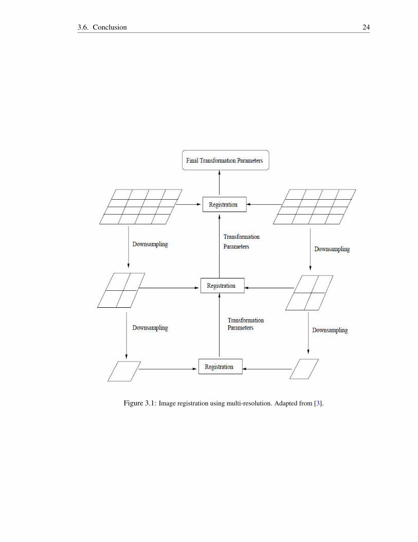
3.6. Conclusion 24
Figure 3.1: Image registration using multi-resolution. Adapted from [3].
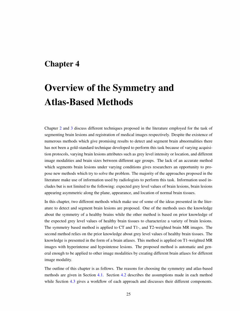
Chapter 4
Overview of the Symmetry andAtlas-Based Methods
Chapter 2 and 3 discuss different techniques proposed in the literature employed for the task of
segmenting brain lesions and registration of medical images respectively. Despite the existence of
numerous methods which give promising results to detect and segment brain abnormalities there
has not been a gold-standard technique developed to perform this task because of varying acquisi-
tion protocols, varying brain lesions attributes such as grey level intensity or location, and different
image modalities and brain sizes between different age groups. The lack of an accurate method
which segments brain lesions under varying conditions gives researchers an opportunity to pro-
pose new methods which try to solve the problem. The majority of the approaches proposed in the
literature make use of information used by radiologists to perform this task. Information used in-
cludes but is not limited to the following: expected grey level values of brain lesions, brain lesions
appearing asymmetric along the plane, appearance, and location of normal brain tissues.
In this chapter, two different methods which make use of some of the ideas presented in the liter-
ature to detect and segment brain lesions are proposed. One of the methods uses the knowledge
about the symmetry of a healthy brains while the other method is based on prior knowledge of
the expected grey level values of healthy brain tissues to characterize a variety of brain lesions.
The symmetry based method is applied to CT and T1-, and T2-weighted brain MR images. The
second method relies on the prior knowledge about grey level values of healthy brain tissues. The
knowledge is presented in the form of a brain atlases. This method is applied on T1-weighted MR
images with hyperintense and hypointense lesions. The proposed method is automatic and gen-
eral enough to be applied to other image modalities by creating different brain atlases for different
image modality.
The outline of this chapter is as follows. The reasons for choosing the symmetry and atlas-based
methods are given in Section 4.1. Section 4.2 describes the assumptions made in each method
while Section 4.3 gives a workflow of each approach and discusses their different components.
25

4.1. Motivation for Choosing Knowledge-Driven Methods 26
Section 4.4 concludes the chapter.
4.1 Motivation for Choosing Knowledge-Driven Methods
Anomaly detection and segmentation methods can be categorized under two umbrella terms, namely
knowledge-driven and data-driven methods. Knowledge-driven methods utilize prior anatomical
knowledge about the properties of healthy brain structures to guide segmentation, while data-driven
methods are supervised or unsupervised and statistical in nature. The symmetry-based and atlas-
based methods are classified as knowledge-driven methods. Figures 4.1 and 4.2 show a graphical
illustration under which knowledge and data-driven methods are likely to succeed or fail using
prototype axial slices with a simulated brain tumors at different locations.
Data-driven methods (supervised and unsupervised) are limited to the problem they are designed
to solve and often fail to give correct results in cases where there is an overlapping intensity dis-
tribution between healthy tissue and abnormal tissue, as shown in Figure 4.2. Additionally, when
they are used on a different image modality they need to be re-engineered since they misclassify
normal and tumorous tissues. The cross variability of intensity distribution between healthy and
abnormal tissues still remains a challenge within the supervised methods, and some of the unsu-
pervised methods have adopted the selection of seed points for initialization though it limits such
methods not to be fully automatic.
The symmetry method works well when the lesion is localized in one hemisphere as shown in the
first image of Figures 4.1 and 4.2. In cases where the lesions are symmetrically placed on both
hemispheres as illustrated in the second image of Figures 4.1 and 4.2, this method is likely to fail.
Moreover if the lesion is large enough to cross the symmetry axis, as depicted in the last image of
Figures 4.1 and 4.2, it becomes difficult to use the symmetry alone to detect abnormal tissues. This
method is applicable to different image modalities and need not be redesigned or retrained when
it is subjected to such variations. The same set of rules can be employed to detect and segment
asymmetric brain tissues without human input.
An atlas-based method works correctly only when it is applied to images of modality similar to
those it was constructed with. It is expected to mark the location of the brain lesion, regardless of
whether the lesion is symmetric or not, or if there is an overlapping intensity distribution between
the lesion and healthy tissue. However, when it is employed on subjects of a different modality it
can misclassify healthy and abnormal tissues. This problem can be solved by constructing a multi-
modality brain atlas without a need to re-engineer or redesign. Given the sample atlas depicted in
Figure 4.3, this method is likely to delineate the abnormalities illustrated in Figure 4.1 and 4.2 by
analyzing either the intensity difference between the test image and the atlas or the displacement
field after applying the registration.
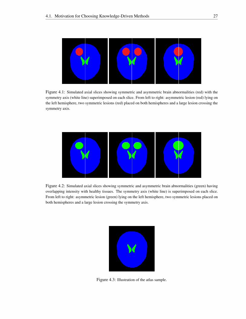
4.1. Motivation for Choosing Knowledge-Driven Methods 27
Figure 4.1: Simulated axial slices showing symmetric and asymmetric brain abnormalities (red) with thesymmetry axis (white line) superimposed on each slice. From left to right: asymmetric lesion (red) lying onthe left hemisphere, two symmetric lesions (red) placed on both hemispheres and a large lesion crossing thesymmetry axis.
Figure 4.2: Simulated axial slices showing symmetric and asymmetric brain abnormalities (green) havingoverlapping intensity with healthy tissues. The symmetry axis (white line) is superimposed on each slice.From left to right: asymmetric lesion (green) lying on the left hemisphere, two symmetric lesions placed onboth hemispheres and a large lesion crossing the symmetry axis.
Figure 4.3: Illustration of the atlas sample.

4.2. Assumptions 28
4.2 Assumptions
There are three fundamental assumptions in the asymmetry quantification method.
1. The healthy brain tissue is symmetric in both hemispheres with minimal shifting expected
due to the swelling of the brain lesions such as meningiomas.
2. The lesions do not cross the symmetry axis and are localized in one of the hemispheres.
3. Also they have intensity values different from their surrounding healthy brain tissues.
For analysis in atlas-based methods the following assumptions are made for normalization of dif-
ferent subjects.
1. Because of the different shapes and sizes of patient’s brains across age or race groups, a
population specific brain atlas is constructed under the prime assumption that the topological
structures of the brain remain invariant among normal subjects.
2. The affine registration is capable of resolving global misalignment and size between different
subjects.
3. A nonrigid registration resolves local shape difference between internal structures of the
subjects. The registration algorithms assume the same intensity for corresponding brain
structures in the two images to be aligned.
4.3 Outline of the Proposed Methods
In this section a detailed workflow of each method is presented, so that subsequent chapters dis-
cussing the implementations can be easily understood. The atlas is constructed from the set of
healthy brain images which have been aligned onto one coordinate space.
4.3.1 Anomaly Detection Using Symmetry Analysis Method
The symmetry analysis method is based on the assumption that the brain appears symmetrical
and the symmetry is breached in cases where various conditions of brain pathologies occur. The
conditions include brain lesions appearing only on one side of the brain hemisphere or appearing
on both hemispheres but at different locations. Figure 4.4 illustrates a series of steps associated
with the symmetry-based method. The major components involved in this approach include: (1)
detection of the symmetry plane, (2) tilt correction and (3) asymmetry quantification.
Detection of the Symmetry Plane: the mid-sagittal plane (MSP) is the plane dividing the brain
into similar hemispheres. This is the main building block for asymmetry analysis since all the
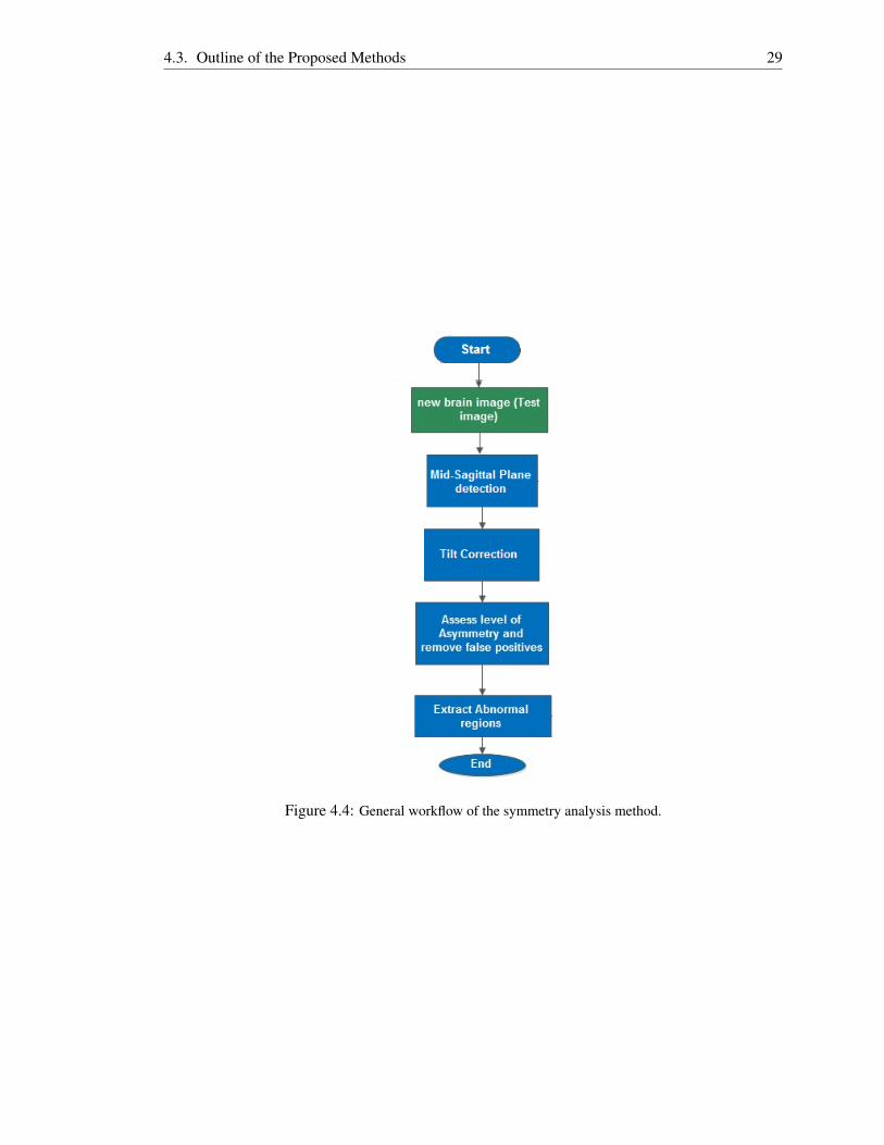
4.3. Outline of the Proposed Methods 29
Figure 4.4: General workflow of the symmetry analysis method.
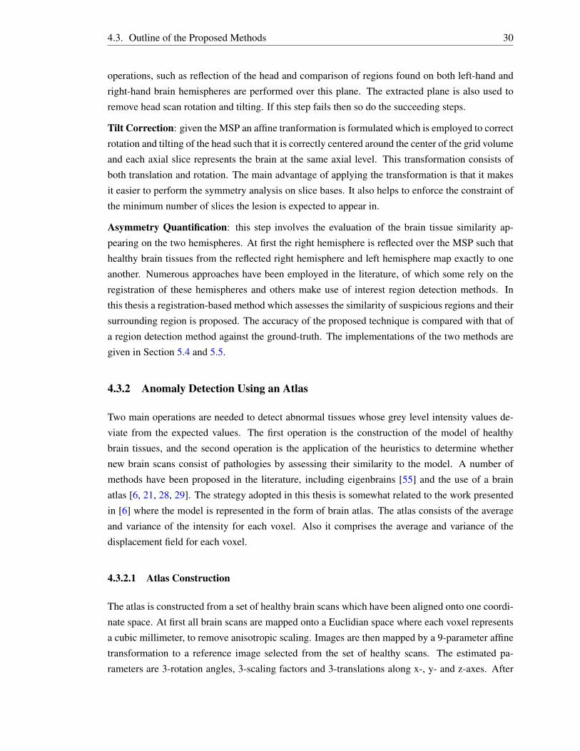
4.3. Outline of the Proposed Methods 30
operations, such as reflection of the head and comparison of regions found on both left-hand and
right-hand brain hemispheres are performed over this plane. The extracted plane is also used to
remove head scan rotation and tilting. If this step fails then so do the succeeding steps.
Tilt Correction: given the MSP an affine tranformation is formulated which is employed to correct
rotation and tilting of the head such that it is correctly centered around the center of the grid volume
and each axial slice represents the brain at the same axial level. This transformation consists of
both translation and rotation. The main advantage of applying the transformation is that it makes
it easier to perform the symmetry analysis on slice bases. It also helps to enforce the constraint of
the minimum number of slices the lesion is expected to appear in.
Asymmetry Quantification: this step involves the evaluation of the brain tissue similarity ap-
pearing on the two hemispheres. At first the right hemisphere is reflected over the MSP such that
healthy brain tissues from the reflected right hemisphere and left hemisphere map exactly to one
another. Numerous approaches have been employed in the literature, of which some rely on the
registration of these hemispheres and others make use of interest region detection methods. In
this thesis a registration-based method which assesses the similarity of suspicious regions and their
surrounding region is proposed. The accuracy of the proposed technique is compared with that of
a region detection method against the ground-truth. The implementations of the two methods are
given in Section 5.4 and 5.5.
4.3.2 Anomaly Detection Using an Atlas
Two main operations are needed to detect abnormal tissues whose grey level intensity values de-
viate from the expected values. The first operation is the construction of the model of healthy
brain tissues, and the second operation is the application of the heuristics to determine whether
new brain scans consist of pathologies by assessing their similarity to the model. A number of
methods have been proposed in the literature, including eigenbrains [55] and the use of a brain
atlas [6, 21, 28, 29]. The strategy adopted in this thesis is somewhat related to the work presented
in [6] where the model is represented in the form of brain atlas. The atlas consists of the average
and variance of the intensity for each voxel. Also it comprises the average and variance of the
displacement field for each voxel.
4.3.2.1 Atlas Construction
The atlas is constructed from a set of healthy brain scans which have been aligned onto one coordi-
nate space. At first all brain scans are mapped onto a Euclidian space where each voxel represents
a cubic millimeter, to remove anisotropic scaling. Images are then mapped by a 9-parameter affine
transformation to a reference image selected from the set of healthy scans. The estimated pa-
rameters are 3-rotation angles, 3-scaling factors and 3-translations along x-, y- and z-axes. After

4.4. Conclusion 31
employing the affine transformation a nonrigid registration is also applied to correct any slight de-
formation that may result between the reference image and other images. After aligning the entire
dataset onto the same coordinate frame, the atlas is developed.
4.3.2.2 Detecting Anomalies
Evaluating the similarity between a new brain scan (taken in axial format) and the atlas requires
the scan to be aligned onto the atlas space. Two different approaches are followed to estimate the
affine transformation between the new scan and the atlas. One approach is based on registering
full scans and the other is based on registering partial scans. Aligning partial data to atlas space
is a challenging task due to a lot of missing data between the subject and the atlas. The procedure
to estimate the transformation using a 2D affine transformation between midsagittal and coronal
slices is discussed below.
The affine transformation between partial scan and the atlas is computed from a set of 2D affine
transformations estimated by aligning mid-sagittal and coronal slices of the scan and atlas. At
first a mid-sagittal slice from two volumes is used to find the transformation that scales, positions
and rotates sagittal slices of the subject to match sagittal slices of the atlas. The same principle is
applied to coronal slices to find the transformation which scales coronal slices of these volumes to
the same size. The two transformations are then combined and the final transformation is applied
to the data. Registering a full scan onto the atlas space requires the estimation of a 3D affine
transformation which is determined in a similar fashion to that employed when constructing the
atlas. After applying the affine transformation a nonrigid registration is performed to remove local
displacement of brain tissues. A drawback of nonrigid registration is that it introduces artifacts in
cases where brain structures between two images do not match correctly. This often occurs in the
presence of abnormal tissues in the subject which are not present in the brain atlas.
After mapping the test image into the atlas space, the corresponding voxels between the registered
scan and atlas are compared to determine voxels with intensity values deviating from the expected
values. These voxels are classified as abnormal and mark the proposed location of the brain tumor.
4.4 Conclusion
This chapter reviewed different components associated with the symmetry-based and atlas-based
methods. It also provided reasons for choosing these two approaches. The assumptions have been
stated for each method. The implementation and evaluation of the symmetry-based methods on
T1- and T2-weighted MR images are given in Chapter 5. Chapter 6 describes the implementation
and evaluation of the atlas-based method on T1-weighted MR images.

Chapter 5
Symmetry Plane Detection andAsymmetry Quantification in CT andMR Images
This chapter gives a detailed description of the method used for extraction of the mid-sagittal
plane (MSP) and detection of brain lesions using asymmetry. A 2D or 3D object is said to have
a bilateral symmetry if there exists a line or plane respectively that separates the object into two
identical parts. The asymmetry quantification method used addresses a variety of brain pathologies
in CT and MR images which appear asymmetric along the inter-hemispheric (longitudinal) fissure
bisecting the brain, the MSP in this case, into similar hemispheres. The following three steps are
performed to detect and segment brain lesions: (1) detection of the MSP, (2) tilt correction and (3)
asymmetry quantification.
The detection of the MSP is modeled as an optimization problem which minimizes the similarity
measure to find the optimal values of the symmetry plane parameters. It is based on the assumption
that the scan has a single region of interest which is ellipsoidal in shape. To detect and segment
asymmetric brain lesions from 3D MR and CT images, two asymmetry quantification methods have
been implemented. They are based on the assumption that healthy human brain tissues appear
symmetrical with respect to the MSP and the symmetry is violated by the presence of lesions.
The first technique is a registration-based method which aligns healthy brain tissues from the two
hemispheres while the second one is based on 2D region detection.
The outline of this chapter is as follows. Section 5.1 describes the symmetry axis in 2D images.
Section 5.2 discusses the MSP detection algorithm in detail while Section 5.3 gives a description
of the procedure followed to transform a tilted head scan so that each axial slice represents the
brain at the same axial level. Sections 5.4 and 5.5 describe asymmetry analysis methods based on
registration and region of interest detection respectively. Section 5.6 concludes with results and
32
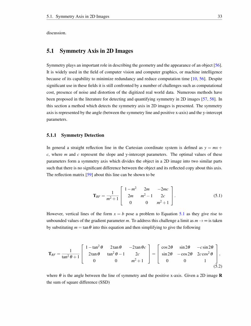
5.1. Symmetry Axis in 2D Images 33
discussion.
5.1 Symmetry Axis in 2D Images
Symmetry plays an important role in describing the geometry and the appearance of an object [56].
It is widely used in the field of computer vision and computer graphics, or machine intelligence
because of its capability to minimize redundancy and reduce computation time [10, 56]. Despite
significant use in these fields it is still confronted by a number of challenges such as computational
cost, presence of noise and distortion of the digitized real world data. Numerous methods have
been proposed in the literature for detecting and quantifying symmetry in 2D images [57, 58]. In
this section a method which detects the symmetry axis in 2D images is presented. The symmetry
axis is represented by the angle (between the symmetry line and positive x-axis) and the y-intercept
parameters.
5.1.1 Symmetry Detection
In general a straight reflection line in the Cartesian coordinate system is defined as y = mx +
c, where m and c represent the slope and y-intercept parameters. The optimal values of these
parameters form a symmetry axis which divides the object in a 2D image into two similar parts
such that there is no significant difference between the object and its reflected copy about this axis.
The reflection matrix [59] about this line can be shown to be
TRF =1
m2 +1
1−m2 2m −2mc
2m m2−1 2c
0 0 m2 +1
. (5.1)
However, vertical lines of the form x = b pose a problem to Equation 5.1 as they give rise to
unbounded values of the gradient parameter m. To address this challenge a limit as m→∞ is taken
by substituting m = tanθ into this equation and then simplifying to give the following
TRF =1
tan2 θ +1
1− tan2 θ 2tanθ −2tanθc
2tanθ tan2 θ −1 2c
0 0 m2 +1
=
cos2θ sin2θ −csin2θ
sin2θ −cos2θ 2ccos2 θ
0 0 1
,(5.2)
where θ is the angle between the line of symmetry and the positive x-axis. Given a 2D image Rthe sum of square difference (SSD)

5.2. Mid-Sagittal Plane Detection 34
SSD(u) =12||R−F(u)||2L2
, (5.3)
is used as the symmetry measure to determine the closeness of R to its reflected copy F(u) =R(TRF(x,u)) where u= [θ ,c]T and x= [x,y]T . The optimal values of θ and c are found by omitting
the z-axis and employing the Levenberg-Marquardt optimization and multiresolution method as
described in Section 5.2.6.
5.1.2 Symmetry Detection Results
The method was tested on randomly selected axial slices of MR and CT scans. It was also tested
on simulated binary images. A total of nine test images were used: three images from MR, CT
and binary images. In some datasets bright and dark asymmetric rectangular regions, of dimen-
sions 40× 20 pixels, are created and overlaid on the test images to determine if the presence of
asymmetry lesions could affect the accuracy of the method. Figure 5.1 illustrates the results for the
best symmetry axis found in these images. From these results the conclusion that can be drawn is
that the tested method can estimate a line of symmetry regardless of the presence of asymmetric
regions. However, the algorithm sometimes is trapped if the global minimum is far from the initial
guess or one of the object’s symmetrical halves is more sheared than the other. This can be seen in
the right-bottom binary image of Figure 5.1. The method is extended to 3D in the next section to
detect the MSP in 3D brain CT and MR images.
5.2 Mid-Sagittal Plane Detection
The extraction of the MSP is formulated as an optimized registration problem in a manner similar
to the 2D case just described. Given the brain MR or CT scan R and initial values of the candidate
plane parameter a transformation is formed which is used to reflect R over the plane to create a
new scan F. The method searches for the optimal plane parameter values that minimizes the sum
of square difference (SSD) between R and F.
5.2.1 Geometry of the MSP
There are various ways to represent a plane in 3D Cartesian coordinates. The equation of the plane
can be deduced from three non-collinear points (p1,p2,p3) lying on the plane [30]. It can also be
deduced from the given point p0 = [x0,y0,z0]T that lies on the plane and a perpendicular vector, n,
to the plane [10]. A general equation of the plane is given as
Ax+By+Cz+D = 0, (5.4)
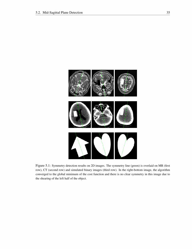
5.2. Mid-Sagittal Plane Detection 35
Figure 5.1: Symmetry detection results on 2D images. The symmetry line (green) is overlaid on MR (firstrow), CT (second row) and simulated binary images (third row). In the right-bottom image, the algorithmconverged to the global minimum of the cost function and there is no clear symmetry in this image due tothe shearing of the left half of the object.
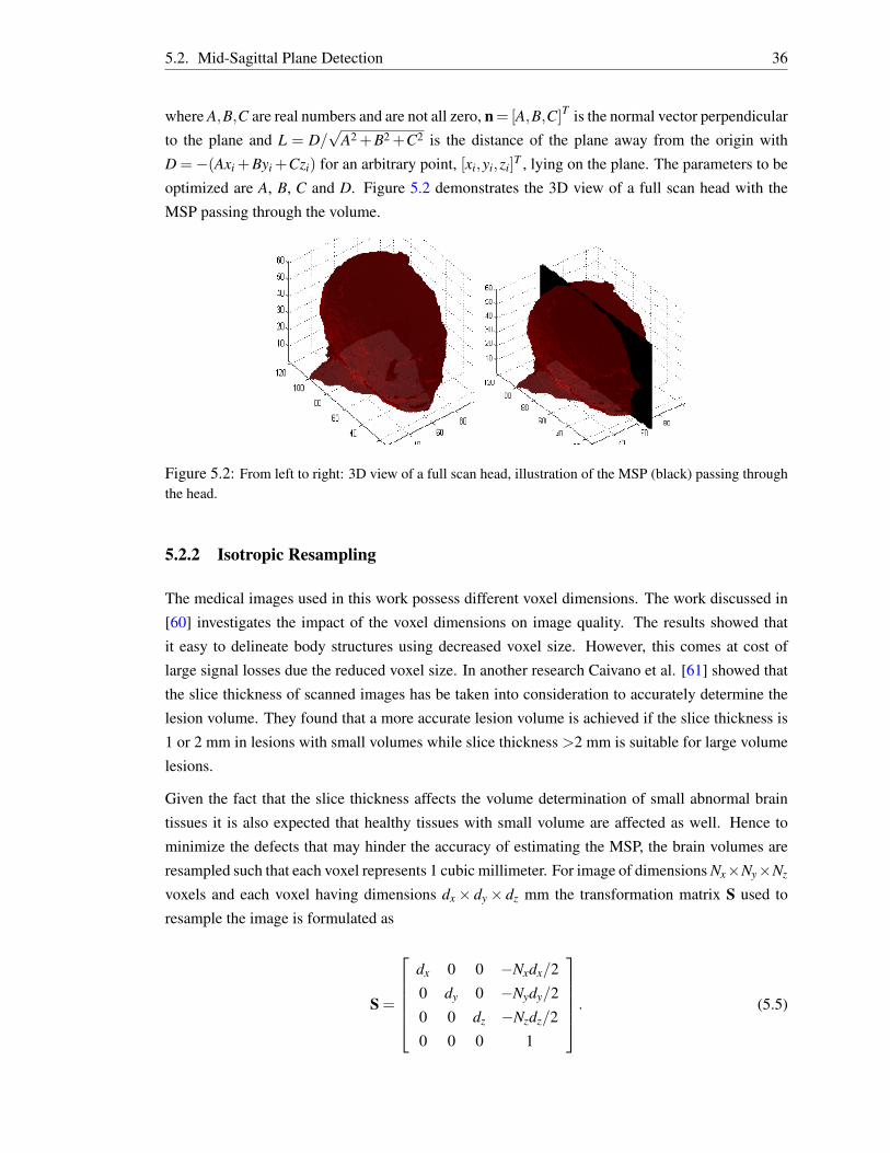
5.2. Mid-Sagittal Plane Detection 36
where A,B,C are real numbers and are not all zero, n= [A,B,C]T is the normal vector perpendicular
to the plane and L = D/√
A2 +B2 +C2 is the distance of the plane away from the origin with
D =−(Axi +Byi +Czi) for an arbitrary point, [xi,yi,zi]T , lying on the plane. The parameters to be
optimized are A, B, C and D. Figure 5.2 demonstrates the 3D view of a full scan head with the
MSP passing through the volume.
Figure 5.2: From left to right: 3D view of a full scan head, illustration of the MSP (black) passing throughthe head.
5.2.2 Isotropic Resampling
The medical images used in this work possess different voxel dimensions. The work discussed in
[60] investigates the impact of the voxel dimensions on image quality. The results showed that
it easy to delineate body structures using decreased voxel size. However, this comes at cost of
large signal losses due the reduced voxel size. In another research Caivano et al. [61] showed that
the slice thickness of scanned images has be taken into consideration to accurately determine the
lesion volume. They found that a more accurate lesion volume is achieved if the slice thickness is
1 or 2 mm in lesions with small volumes while slice thickness >2 mm is suitable for large volume
lesions.
Given the fact that the slice thickness affects the volume determination of small abnormal brain
tissues it is also expected that healthy tissues with small volume are affected as well. Hence to
minimize the defects that may hinder the accuracy of estimating the MSP, the brain volumes are
resampled such that each voxel represents 1 cubic millimeter. For image of dimensions Nx×Ny×Nz
voxels and each voxel having dimensions dx× dy× dz mm the transformation matrix S used to
resample the image is formulated as
S =
dx 0 0 −Nxdx/2
0 dy 0 −Nydy/2
0 0 dz −Nzdz/2
0 0 0 1
. (5.5)
5.2. Mid-Sagittal Plane Detection 37
The new dimensions of the transformed image is N′x×N
′y×N
′z where N
′x = Nxdx, N
′y = Nydy and
N′z = Nzdz. Backward Cubic interpolation is employed remove the holes that arises between the
voxels of the resampled image.
5.2.3 Feature Space
The registration between the original brain image and its reflected copy uses an intensity-based
approach. The images are aligned using their raw voxel intensity values, hence preprocessing steps
for feature extraction are not required. The drawback of this approach is the high computational
cost since the entire set of image information is used. A common approach used to speed up
intensity-based methods is to use a subset of voxels sampled on a uniform grid or a defined mask
image locating the region of interest supplied by the user [49]. In this work a subset of voxels
sampled on a uniform 3D grid is adopted since it limits human interaction.
5.2.4 3D Reflection Transformation Matrix
The registration process requires a transformation matrix to align one image onto another. In the
MSP detection problem a 4D reflection matrix TRF is used to reflect the 3D medical image over
the candidate symmetry plane. The general equation of TRF is deduced from Equation (5.4) as
follows. Given a point p0 = [x0,y0,z0]T , to be reflected over the plane, a line that passes through
p0 and perpendicular to plane is defined as
r = p0+αn = [x0,y0,z0]T +α [A,B,C]T = [x0 +αA,y0 +αB,z0 +αC]T , (5.6)
where α is distance in the direction of the normal to the plane. Equation (5.6) is substituted into
Equation (5.4) to solve for α which is substituted back into Equation (5.6) to find the intersection
point p1 = [x0 +αAx0,y0 +αBy0,z0 +αCz0]T of the line and the plane. The intersection point acts
as an intermediate point between the original point p0 and its reflected copy p2. The value for α is
calculated as
α =−(Ax0 +By0 +Cz0 +DA2 +B2 +C2 ), (5.7)
where A,B,C are not all zero. Hence, knowing the coordinates of p1, the coordinates of p2 are
obtained as p2 = 2p1−p0 [62]. Using homogeneous coordinates [44] p2 can be represented by a
4×4 matrix and 4×1 vector point as follows
5.2. Mid-Sagittal Plane Detection 38
p2=TRFp0 =1Λ
Λ−2A2 −2AB −2AC −2AD
−2AB Λ−2B2 −2BC −2BD
−2AC −2BC Λ−2C2 −2CD
0 0 0 Λ
x0
y0
z0
1
, (5.8)
where Λ = A2 +B2 +C2 and p0 = [x0,y0,z0,1]T .
5.2.5 Similarity Measure
The original MR or CT image R and its reflected copy F = R(TRF(x,u)) represent images of the
same modality for u = [A,B,C,D]T . The sum of square difference (SSD) is used as the similarity
criterion to measure how well the two images match one another. SSD is chosen since it is simple
to compute and uses the whole image information [47]. This measure is minimized to find the
optimal values of plane parameters. SSD between the R and F is given as
SSD(u) =12||R−F(u)||2L2
=12
f(u)T f(u), (5.9)
where f(u) = R(x)−R(TRF(x,u)), TRF is the reflection matrix, and x = [x,y,z]T is an abitrary 3D
point.
5.2.6 Optimization Using Levenberg-Marquardt (LM) Method
The Levenberg-Marquardt method is utilized to minimize the SSD between the MR or CT image
R and its reflected copy F. This is a nonlinear least square problem in which the function to be
minimized is represented as the sum of square difference of the corresponding voxels in the two
images [51]. LM is adopted in this work as an optimization method due to the fact that it inherits
the speed of Gauss-Newton algorithm and the stability of Steepest Descent to find the minimum of
the similarity measure SSD [44, 45, 53].
The vector parameter used to formulate the reflection transformation is described by u= [A,B,C,D]T
=[u1,u2,u3,u4
]T . This vector is updated at each iteration after computing the derivative of the
SSD with respect to u. As it can be seen from Equation 5.9 F(u) = R(TRF(x,u)) is a function of
u. This means if u is perturbed by a tiny amount, F is also expected to change. Hence the derivative
of F with respect to u is used to estimate the Jacobian matrix J(u) [44]. Given the initial parameter
value u0 =[u1
0,u20,u
30,u
40]T the derivative of F is carried out numerically to compute the Jacobian
matrix J(u) as described in [44]:
Ji j(u) = ∂F j/∂ui. (5.10)
Numerical differentiation of Equation (5.10) computed using the forward difference method is as

5.2. Mid-Sagittal Plane Detection 39
follows
Ji j(u) =(
F(u+δ~ui)−F(u))/δ , (5.11)
for 1≤ i≤ 4, 1≤ j≤ NxNyNz, and where ~ui is the unit direction vector along the ui-axis. A routine
is developed in which R is reflected over the candidate plane to generate a new image Fuievery
time after each independent variable ui is modified by δ . The value for δ is set to the maximum
of |10−4ui| and 10−6 as described in [44]. The same routine is used to compute J(u) to improve
convergence and computation speed slightly [44]. The Hessian matrix is constructed directly from
the first derivatives, and its diagonal elements are augmented as described in Section 3.4.5. The
search direction dk is also computed as described in Section 3.4.5. If the newly computed value of
the vector parameter uk+1=uk +dk reduces the error function, then the new parameter is accepted,
the damping factor µ is reduced by a factor of 10, and the algorithm continues to the next iteration if
convergence is not reached. Otherwise µ is increased by a factor of 10 if uk+1 leads to an increased
error and equations are solved again with the new value of µ . The damping factor µ is updated
based on the value of the gain ratio as described in Section 3.4.5. The summary of the algorithm
consists of the following steps.
Input: (MR or CT scan in axial format R, initial parameter [u0,µ], stopping criterion [kmax,ε1])
Output: ( u∗k = [A,B,C,D]T )
Algorithm
Begin
Step 0: Load input variables into memory.
Step 1: while k < kmax, do
Step 2: Compute J using forward difference.
Step 3: Augment diagonal elements of the Hessian estimate by µ .
Step 4: Solve for the search direction, dk, from augmented equations.
Step 5: if ||dk||< ε1, Goto Step 9.
Step 6: Update plane parameter temporarily, v = uk +dk, and compute gain ratio ρ .
Step 7: If ρ > 0, increase iterations by 1 (k = k+1), decrease damping factor by 10
(µ = µ/10), permanently update plane parameters (uk = v). Goto Step 1.
Step 8: Increase damping factor by 10 (µ = 10µ). Goto Step 3.
Step 9: Return final results after convergence is reached.
End
5.2. Mid-Sagittal Plane Detection 40
The algorithm is slow for large image sizes and is often trapped in the local minima if the initial
guess of the plane parameter value is far from the optimal value. Therefore, to provide a good
initial guess of plane parameter value a multi-resolution is applied.
5.2.7 Multi-Resolution
Multi-resolution is adopted to speed up the registration problem and to provide a reliable guess
of the plane parameter vector u [10, 30, 45]. The image of interest R is downsampled to low
resolution images which are used to estimate the plane parameters with reduced computational
load [30, 49, 45]. Given that the dimensions of R at the highest level L are Nx×Ny×Nz, the size of
the image at the coarser level l is obtained by down scaling the image at the finest level by a scale
factor of 2L−l , followed by the interpolation. In this work the total number of levels is set to four.
At each level l, the Levenberg-Marquardt method described in Section 5.2.6 is used to compute the
reflection transformation while estimating the optimal parameters of the plane up to some defined
tolerance or number of iterations.
The initial guess of plane parameters is used at the coarsest level and the parameters are updated
after each iteration. In this thesis three initial guesses, (u01,u02,u03) of plane parameter are used
at the coarsest level to reduce the problem of the algorithm being trapped in a local minimum. The
initial guess that leads to convergence with the minimum error between the three is considered as
the best guess and is used in succeeding levels. With the assumption that the brain scan is in axial
format u01 = [0,1,0,Ny/2]T is the sagittal plane that divides the volume lattice into two halves with
equal size. The guesses u02 and u03 are derived by rotating u01 with the rotational angle θ = 25◦
and θ = −25◦ respectively about the z-axis. The value of the rotational angle is set empirically
based on the observation that LM gets trapped in a local minimum if the head is severely tilted.
When convergence is reached the optimum results obtained are modified and used as the initial
guess at the next level. In this problem only the last parameter D is modified while others remain
unchanged. Since the size of the image at the next level is twice larger than the size at the coarser
level so does the distance of the plane away from the origin. This can be written mathematically as
[A(L−l−1),B(L−l−1),C(L−l−1),D(L−l−1)
]T=[A(L−l),B(L−l),C(L−l),2∗D(L−l)
]T, (5.12)
for 1 ≤ l < L. The whole process continues until the highest level is reached, and the optimal
results found at this level are used as the final estimate of the MSP.
Input: (CT or MR scan in axial format R, initial parameter [u01,u02,u03,µ], stopping criterion
[kmax,ε1,ε2],number of levels Lmax)
Output: ( u∗k = [A,B,C,D]T )
Algorithm
Begin
5.3. Tilt Correction 41
Step 0: Load input variables into memory.
Step 1: downsample R by 2Lmax to get new volume R1.
Step 2: Evaluate the LM method given in 5.2.6 at ( R1, [u01,µ], stopping criterion [kmax,ε1]).
Step 3: Evaluate the LM method given in 5.2.6 at ( R1, [u02,µ], stopping criterion [kmax,ε1]).
Step 4: Evaluate the LM method given in 5.2.6 at ( R1, [u03, ,µ], stopping criterion [kmax,ε1]).
Step 5: Set l = 1 and ul to optimal parameter (in step 3,4 and 5) that converged with the minimum
error.
Step 6: if (l < Lmax), then update ul using equation 5.12.
Step 7: while l ≤ Lmax, do
Step 8: down sample R by 2Lmax−l to get new volume R1.
Step 9: Evaluate the LM method given in Section 5.2.6 at ( R1, [u1,µ],Stopping criterion
[kmax,ε1]).
Step 10: if (l < Lmax), then update ul using Equation 5.12.
Step 11:l = l +1, update the level. Goto Step 7.
Step 12: Return final results after convergence is reached at level l = Lmax.
End
5.3 Tilt Correction
The orientation of the patient sometimes leads the scanned head appearing tilted about y-axis or
rotated about z-axis. The rotations about x-axis has no impact on repositioning tissues that are
on the same axial level. The tilted and rotated image makes it difficult, even for a radiologist, to
perform asymmetry analysis as corresponding regions might be at different axial levels. Hence the
MSP is used to align the head with the volume lattice and center it within the volume. Given the
candidate plane Equation (5.4) the rotation matrices Rz, Ry and the translation matrix Tl can easily
be determined. The rotation transformations Rz and Ry correct the rotations of the head about
the z-axis and the y-axis respectively while the translation transformation Tl defines the center of
rotation. The rotational angles β and φ are obtained by taking a dot product between the plane
normal vector and unit vectors XY = [0,0,1]T and XZ = [0,1,0]T respectively. The unit vectors,
[0,0,1]T and [0,1,0]T , are the normal vectors of the XY and XZ planes respectively. The final
rotation MRis given as follows:

5.4. Asymmetry Quantification Using Registration 42
MR = RzRy =
cosφ −sinφ 0 0
sinφ cosφ 0 0
0 0 1 0
0 0 0 1
cosβ 0 sinβ 0
0 1 0 0
−sinβ 0 cosβ 0
0 0 0 1
. (5.13)
The translation matrixTl is given as shown below:
Tl1 =
1 0 0 Tx
0 1 0 Ty
0 0 1 Tz
0 0 0 1
, (5.14)
where (Tx,Ty,Tz) is the center of rotation. Given the center of the image grid C = (x,y,z), the center
of the rotation is calculated as the midway point between C and the reflected copy of C over the
plane. The final rigid transformation matrix is given as MA = TlMRT−1l . Cubic interpolation is
used to get rid of holes and produce an acceptable images. Figure 5.3 illustrates results after tilt
corrections are performed on a MR and a CT dataset.
Figure 5.3: Results for CT and MRI scan after tilt correction: (first row) misaligned scans with the MSPoverlaid on each slice; (second row) corresponding slices after tilt correction.
5.4 Asymmetry Quantification Using Registration
A fully automatic method to detect and segment brain tumors in 3D CT and MR scans using sym-
metry analysis is proposed. The technique presented here follows the same principle as the work
described in [34] with the assumption that tumorous tissues are not symmetrically placed in both
hemispheres. A nonrigid registration is used to correct slight displacement of corresponding voxels
of the left hemisphere and a reflected copy of the right hemisphere. Analysis of intensity differ-
ences followed by a thresholding technique is employed to determine the presence of asymmetric
tissues. Constraints are then applied to remove false positive regions. For illustration purpose in

5.4. Asymmetry Quantification Using Registration 43
each step a 3D CT data from iThemba LABS is used.
5.4.1 Nonrigid Registration
An aligned MR or CT image I is divided into two hemispheres: the left hemisphere R and the
reflected copy of the right hemisphere F . Though the brain might appear largely symmetrical
there is a tendency of the right frontal lobe to be larger than the left one and the left occipital
lobe to be larger than the right one [63]. Hence nonrigid registration is applied to correct these
differences.
The Medical Image Registration Toolbox (MIRT) implemented in MATLAB is used [43]. It is
made freely available for research purposes. The toolbox implements both 2D and 3D nonrigid
image registration. It also has multiple similarity measures such as SSD, MI, normalized mutual
information (NMI), residual complexity (RC) and many others already implemented. More infor-
mation about MIRT can be found in [43]. The following settings have been used based on the
results presented in [43]. The choice of similarity measure used is SSD since the hemispheres to
be registered are of the same modality and it is fast to compute. A three-level multi-resolution
pyramid is also adopted to speed up the registration and increase accuracy. The maximum num-
ber of iterations is set to 100 to avoid the infinite loop while the tolerance between the previous
error measure and the current is set to 6−8 as the stopping criteria. Figure 5.4 depicts the image
difference between left and right hemispheres before and after registration:
Figure 5.4: Results for image difference before and after applying nonrigid registration. From left to right:(1) axial slice from left hemisphere, (2) right hemisphere before registration, (3) registered right hemisphere,(4) intensity difference before registration, (5) intensity difference after registration, (6) suspected lesionsregions for λ = .8 and ζ = .001, (7) lesion regions overlaid on intensity difference. The parameters λ andζ define the maximum intensity difference ratio and threshold between feature vectors respectively and arediscussed later in Section 5.6.3.
5.4.2 Detection of Abnormal Region by Thresholding Image Difference
Since images are already aligned through rigid transformation after tilt correction, large intensity
differences are expected to occur around the regions which are not symmetric. These regions mark
the suspected tumor location in both hemispheres. An intensity difference volume V is used to
describe the absolute intensity difference between the left and the registered right hemisphere. A

5.4. Asymmetry Quantification Using Registration 44
threshold T = λ max(V), where max(V) returns the largest value in V, is applied to V followed
by morphology operations [64], to produce a binary image volume L that estimates the location of
the asymmetric regions. After enforcing the constraints discussed in Section 5.4.3 to removed false
positives, a connected component labeling algorithm based on 3D region growing is used to extract
the remaining regions. The seed point for the region growing method is selected automatically from
the domain of remaining regions.
5.4.3 Removing False Positives
A number of constraints are enforced to penalize unlikely lesion regions and favor the likely ones.
The constraints are set based on the response evaluation criteria in solid tumors (RECIST) standard
published in [65, 66]. RECIST is a diameter-based approach which measures a single-axial slice
containing the largest diameter of the lesion. Though this standard has not been widely adopted
for clinical trials of neck and brain lesions, it is employed in this work to get rid of unmeasurable
lesions. According to RECIST a lesion is declared unmeasurable on CT or MR scans if none of
its axial slice has the longest diameter ≥ 10 mm while a measurable lesion at least has a single
axial slice with the mentioned measurement. Therefore the default minimal false positive lesion
diameter is set to 10 mm to penalize regions with smaller diameters. This number can be changed
manually if lesions of interest have diameters� 10 mm or slice thickness is > 5 mm [65, 66].
The second constraint is based on inter-slice operations. It enforces tumorous region to appear
in at least two successive slices. This means spurious regions that only appear in a single slice
are discarded. Figure 5.5 illustrates left and right hemispheres attached together after nonrigid
registration is applied and the longest diameter (LD) passing across each asymmetric regions.
Figure 5.5: Estimated artificial lesion’s longest diameter (LD): (a) Welded left-hand and right-hand hemi-spheres after performing nonrigid registration, (b) Highly asymmetric regions for λ = .8 andζ = .001, (c)Asymmetric regions (red contour) and LD (green line) for each region superimposed on axial slice, (d)Asymmetric regions with LD≥ 10 mm.
5.4.4 Detect the Ill Hemisphere Using Feature Factors
The analysis so far has been based on the binary volume L which was created by thresholding the
intensity difference volume V. There are still two possibilities that the tumor might be located

5.4. Asymmetry Quantification Using Registration 45
either on the left or right hemisphere. Hence two approaches are used to determine the exact
location of the tumor between the two hemispheres. The first technique is based on the prior
knowledge of the physical properties of brain tissues and tumor appearance. The second is based
on the extraction of first order feature vectors of the region of interest and its surrounding region.
Features are then compared to find which region deviates significantly from its surrounding.
5.4.4.1 Uncover Ill Hemisphere Using Prior Knowledge
With this approach a simple technique that compares mean intensities of the corresponding region
is applied. The idea behind this approach is that a tumorous region always has an intensity that
is different from the surrounding region. Hence given the prior information that lesions appear
hyperintense or hypointense, a region with the highest or lowest intensity mean can be detected.
The results are then used to determine the ill hemisphere.
5.4.4.2 Uncover Ill Hemisphere Without a Priori Knowledge
First-order statistic features describe the information concerning the frequency of the appearance
of grey level in the examined image region [5, 67]. In most cases the grey level values of a lesion
region are often different from those of healthy tissues surrounding it. This means that comparison
of a lesion region’s feature vectors and those of its surrounding area could reveal crucial infor-
mation. The information is used to specify the proposed location of the lesion between the two
hemispheres.
Given a region function G(k) of single variable k = 1,2, ...,N, which can take on discrete values
i = 0,1, ...,M−1, the intensity histogram function H(i) representing, for each intensity i, the total
number of pixels in the whole region having this intensity is given as
H(i) = ∑Nk=1 δ (G(k), i) , δ ( j, i) =
1, j = i
0, j 6= i(5.15)
Dividing the histogram H(i) by a total number of pixel N in a region estimates the probability of
occurrence of the voxels with intensity i = 0,1, ...,M−1 as P(i) = H(i)/N. Hence the first-order
features that can be extracted are defined as:
mean: m = ∑M−1i=0 iP(i), Skewness: m3 =
1σ3 ∑
M−1i=0 (i−m)3P(i),
Variance: σ2 = ∑M−1i=0 (i−m)2P(i), Kurtosis:m4 =
1σ4 ∑
M−1i=0 (i−m)4P(i),
Entropy: H =−∑M−1i=0 P(i) log2(P(i)), Energy:E = ∑
M−1i=0 P(i)2.
(5.16)

5.5. Asymmetry Quantification Using Maximally Stable Extrema Region Detection 46
Put in vector format the feature vectors for the left hand hemisphere region, its surrounding region,
and those that are extracted from the right hand hemisphere are given as vL =[m,σ2,m3,m4,H,E
]T ,
vSL =[m,σ2,m3,m4,H,E
]T , vR =[m,σ2,m3,m4,H,E
]T , and vSR =[m,σ2,m3,m4,H,E
]T . There-
fore given these feature vectors the correct lesion location is determine by evaluating the following
indicator function
f (vL,vSL,vR,vSR) =
2, ||vL−vSL||+ζ < ||vR−vSR||
1, ||vL−vSL||> ζ + ||vR−vSR||
5, otherwise,
(5.17)
where ζ is a predefined threshold, set empirically, determining how well the magnitude of the
difference of the left hemisphere region and its surrounding region feature vectors should differ
from those of the right hand hemisphere. The returned values 2 and 1 show that lesion is precisely
located on the right and left hemispheres respectively. In cases where the difference falls within
the predefined threshold, the value 5 is emitted signaling that the model is unable to determine the
exact pathological hemisphere. Hence the result remains unchanged and is left for the radiologist to
make the final decision. Figure 5.6 shows the suspected location of lesions on the two hemispheres
and the regions surrounding each lesion.
Figure 5.6: Suspected lesions locations on both hemispheres. From left to right: the regions (green)surrounding lesion regions (red) superimposed on the left hemisphere,the regions (green) surrounding lesionregions (red) superimposed on the right hemispheres, most asymmetric regions (red) on the left hemisphere,most asymmetric regions (red) on the right hemisphere.
5.5 Asymmetry Quantification Using Maximally Stable Extrema Re-gion Detection
The approach presented in Section 5.4 depends largely on a nonrigid registration method which
adds more computation time to the process. It is also sensitive to very large intensity differences.
Although this technique might give correct results at the cost of computation, an alternative ap-
proach which does not rely on nonrigid registration is proposed. The new method is based on
detection and comparison of prominent regions between the two hemispheres. Given the left hemi-
sphere R and a reflected copy F of the right hemisphere interest regions are extracted and compared

5.5. Asymmetry Quantification Using Maximally Stable Extrema Region Detection 47
to determine those that are not symmetric over the candidate plane.
5.5.1 Literature on Region Detection
Many of algorithms have been proposed in the literature to detect salient regions and generate
features that are invariant to image transformation [68, 69, 70]. One of the recent affine region
detection methods uses the center-surround distribution distance presented (CSDD) in [40]. This
method is based on comparing features between a central foreground region and a surrounding
ring of background pixels. Hence it detects dark and light blobs surrounded by light and dark
background respectively. Martin et al. [68] describe a new approach for affine invariant region
detection and description. They select high contrast regions as salient regions using a hierarchical
clustering mechanism which is based on the bounded irregular pyramid (BIP). Itti et al. [71] present
a visual attention system. They extract image features using Gaussian pyramids and combine them
into a single topographical saliency map. A single feed-forward neural network is used to select
the most salient region. This method works on RGB images.
Mikolajczyk et al. in [69] provide a review of affine covariant region detectors and compare their
performance on a set of test images under varying imaging conditions. The six investigated detec-
tors include the following: Hessian- and Harris-affine detectors, maximally stable extrema region
(MSER), intensity extrema-based region detector (IBR), edge-based region detector (EBR) and
salient regions. The performances of these detectors are evaluated based on two criteria, namely
repeatability and accuracy. They conclude that the MSER detector, followed by Hessian-Affine de-
tector, outperform the other detectors in various tests. MSER performs well on images containing
homogeneous regions with distinctive boundaries. A detailed description of MSER can be found
in [70] and an open source package [72] which implements MSER is used.
5.5.2 Detection of Interest Region
Healthy and pathological brain tissues usually appear as a connected regions in medical images
unless the image was subjected to noise. Clear boundaries between different tissues can often
be identified especially in MR images, whereas in CT images visible boundaries appear mostly
between healthy and pathological tissues. Therefore given R and F, interest region are extracted
on each slice of the two volumes, using the MSER detection method. The extracted regions are
then compared with their reflected copies to remove false positives and determine those that are
asymmetric. MSER is chosen based on its performance when compared to other interest region
detectors [69]. Figure 5.7 illustrates the most asymmetric regions on axial slices of CT scans.

5.6. Results and Discussion 48
Figure 5.7: Results for MSRE region detection. From left to right: input axial slice from the left hemi-sphere, input axial slice from the right hemisphere, highly asymmetric stable regions detected on the lefthemisphere, highly asymmetric stable regions detected on the right hemisphere for ζ = 0.001.
5.5.3 Removing False Positives
Given a 2D region G1 and its reflected copy G2 the feature vectors given in Section 5.4.4.2 are
extracted and stored in vector v1 and v2. The region G1 is considered to be a true positive if the
Euclidian distance between the two feature vectors is greater than some predefined threshold ζ and
a false negative otherwise. The Euclidian distance is computed by the function f which takes v1
and v2 as its input arguments and outputs either 1 or 0:
f (v1,v2) =
1, ||v1−v2||> ζ
0, otherwise.(5.18)
The constraints discussed in Section 5.4.3 are further applied to remove the remaining false posi-
tives.
5.6 Results and Discussion
This section describes the experiments performed to detect and segment brain tumors using registration-
based and region detection-based asymmetry analysis methods. The two techniques are tested on
real and simulated brain lesions. Simulated brain lesions are created by modifying voxel intensity
values of one of the two hemispheres such that it appears asymmetric over the MSP. The most im-
portant aspect in using artificial lesions is that anomalies of varying intensity values can be created
hence it often makes it easier to test different conditions under which the proposed methods are
likely to succeed or fail.
5.6.1 Dataset Used
Real CT, and both simulated and real MR images scanned in axial format are used in this exper-
iment. CT images are provided by iThemba LABS while MR images are downloaded from the
Internet [1, 2]. Out of seventeen CT scans available only six are full scans and the rest are partial
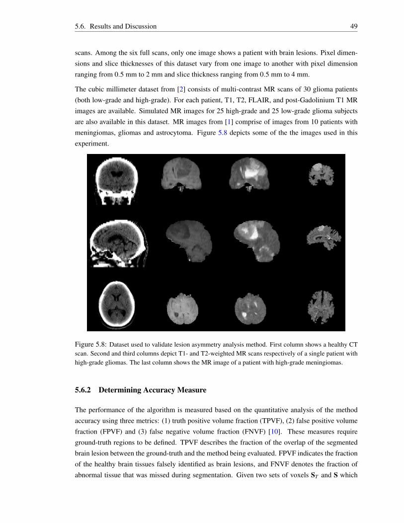
5.6. Results and Discussion 49
scans. Among the six full scans, only one image shows a patient with brain lesions. Pixel dimen-
sions and slice thicknesses of this dataset vary from one image to another with pixel dimension
ranging from 0.5 mm to 2 mm and slice thickness ranging from 0.5 mm to 4 mm.
The cubic millimeter dataset from [2] consists of multi-contrast MR scans of 30 glioma patients
(both low-grade and high-grade). For each patient, T1, T2, FLAIR, and post-Gadolinium T1 MR
images are available. Simulated MR images for 25 high-grade and 25 low-grade glioma subjects
are also available in this dataset. MR images from [1] comprise of images from 10 patients with
meningiomas, gliomas and astrocytoma. Figure 5.8 depicts some of the the images used in this
experiment.
Figure 5.8: Dataset used to validate lesion asymmetry analysis method. First column shows a healthy CTscan. Second and third columns depict T1- and T2-weighted MR scans respectively of a single patient withhigh-grade gliomas. The last column shows the MR image of a patient with high-grade meningiomas.
5.6.2 Determining Accuracy Measure
The performance of the algorithm is measured based on the quantitative analysis of the method
accuracy using three metrics: (1) truth positive volume fraction (TPVF), (2) false positive volume
fraction (FPVF) and (3) false negative volume fraction (FNVF) [10]. These measures require
ground-truth regions to be defined. TPVF describes the fraction of the overlap of the segmented
brain lesion between the ground-truth and the method being evaluated. FPVF indicates the fraction
of the healthy brain tissues falsely identified as brain lesions, and FNVF denotes the fraction of
abnormal tissue that was missed during segmentation. Given two sets of voxels ST and S which

5.6. Results and Discussion 50
represent segmented regions by the ground-truth and the proposed method respectively, accuracy
measures can be defined as
TPVF(S,ST ) =|S∩ST ||ST |
, FPVF(S,ST ) =|S−ST ||ST |
, FNVF(S,ST ) =|ST −S||ST |
. (5.19)
Since asymmetry analysis methods rely heavily on the MSP detection method, a series of exper-
iments are performed to evaluate the algorithm accuracy by subjecting test images to different
conditions such as rotations and artificial asymmetric tumors [10, 73]. The mean angular error
(MAE) and distance error (DE) have been used as the performance measure to quantify the ac-
curacy of the extracted MSP [10]. MAE is computed as the average of the two rotational angle
differences the ground-truth and extracted MSP’s make with the axial and sagittal slices. This
measure evaluates the magnitude of angle deviation, in degrees, that the extracted MSP is from
the ground-truth. DE denotes the distance error between the ground-truth and extracted MSP from
the origin of the image. Given two vectors vT = [φT ,βT ,dT ]T and v = [φ ,β ,d]T which represent
the orientation angles and distance from the origin of the target and extracted MSP, these accuracy
measures are determined as
MAE = (|φT −φ |+ |βT −β |)/2, DE = |dT −d|. (5.20)
5.6.3 Determining Parameter Values
In this section experiments are conducted to determine optimal values of the parameters that have
a major influence on the performance of the segmentation. Throughout the implementation it has
been observed that maximum intensity difference ratio (λ ) and threshold (ζ ) are involved in the
asymmetry analysis method which employs registration and region detection. The parameter λ
defines the relative ratio of the maximum intensity difference between hemispheres and is used
to determine the threshold T (Section 5.4.2). A high value of λ implies that only small intensity
differences exist, hence the brain is likely to be symmetric, while the lower value means large
intensity differences exist hence the brain is likely to be asymmetric. The parameter ζ is used to
describe how well a segmented region from one hemisphere should correspond to its reflected copy
on the other hemisphere.
These parameters are adjusted in a controlled manner until the optimal values are found using
healthy subjects. The optimum values are chosen such that the algorithm tolerates moderate false
positives. The purpose of allowing false positives is to increase the likelihood of the algorithm
detecting low-grade brain lesions whose grey level value is almost identical to the surrounding
healthy brain tissues. Figure 5.9 shows the results of an experiment in which the parameter values
are changed until the desired values are obtained. The second row of this figure shows detected
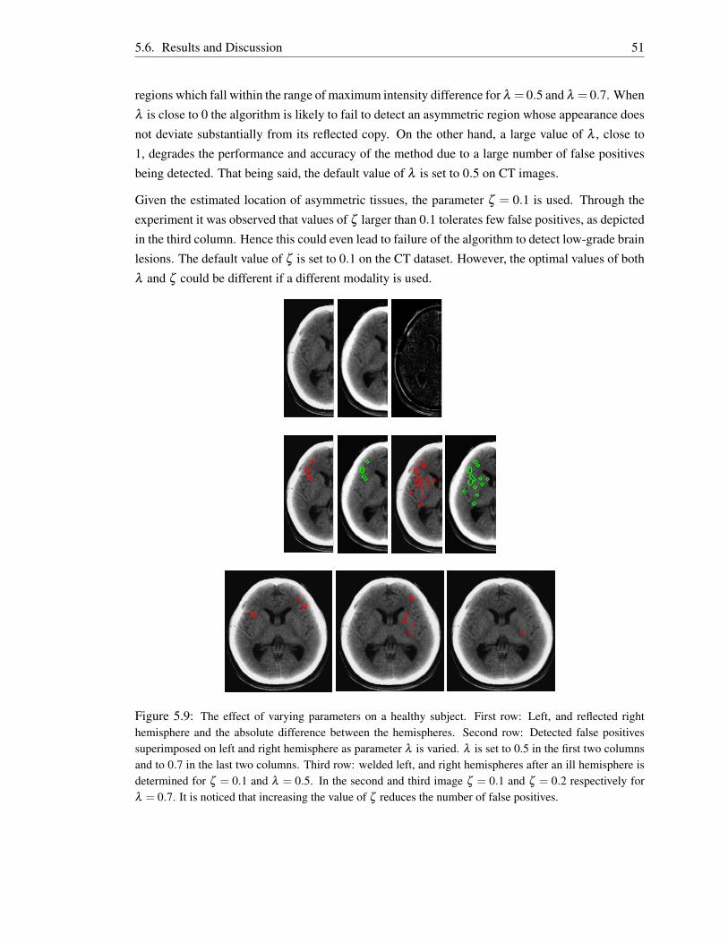
5.6. Results and Discussion 51
regions which fall within the range of maximum intensity difference for λ = 0.5 and λ = 0.7. When
λ is close to 0 the algorithm is likely to fail to detect an asymmetric region whose appearance does
not deviate substantially from its reflected copy. On the other hand, a large value of λ , close to
1, degrades the performance and accuracy of the method due to a large number of false positives
being detected. That being said, the default value of λ is set to 0.5 on CT images.
Given the estimated location of asymmetric tissues, the parameter ζ = 0.1 is used. Through the
experiment it was observed that values of ζ larger than 0.1 tolerates few false positives, as depicted
in the third column. Hence this could even lead to failure of the algorithm to detect low-grade brain
lesions. The default value of ζ is set to 0.1 on the CT dataset. However, the optimal values of both
λ and ζ could be different if a different modality is used.
Figure 5.9: The effect of varying parameters on a healthy subject. First row: Left, and reflected righthemisphere and the absolute difference between the hemispheres. Second row: Detected false positivessuperimposed on left and right hemisphere as parameter λ is varied. λ is set to 0.5 in the first two columnsand to 0.7 in the last two columns. Third row: welded left, and right hemispheres after an ill hemisphere isdetermined for ζ = 0.1 and λ = 0.5. In the second and third image ζ = 0.1 and ζ = 0.2 respectively forλ = 0.7. It is noticed that increasing the value of ζ reduces the number of false positives.
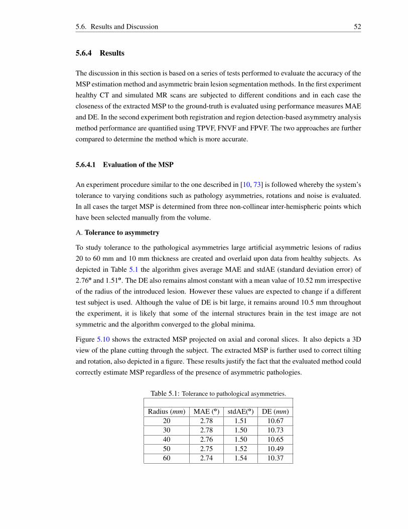
5.6. Results and Discussion 52
5.6.4 Results
The discussion in this section is based on a series of tests performed to evaluate the accuracy of the
MSP estimation method and asymmetric brain lesion segmentation methods. In the first experiment
healthy CT and simulated MR scans are subjected to different conditions and in each case the
closeness of the extracted MSP to the ground-truth is evaluated using performance measures MAE
and DE. In the second experiment both registration and region detection-based asymmetry analysis
method performance are quantified using TPVF, FNVF and FPVF. The two approaches are further
compared to determine the method which is more accurate.
5.6.4.1 Evaluation of the MSP
An experiment procedure similar to the one described in [10, 73] is followed whereby the system’s
tolerance to varying conditions such as pathology asymmetries, rotations and noise is evaluated.
In all cases the target MSP is determined from three non-collinear inter-hemispheric points which
have been selected manually from the volume.
A. Tolerance to asymmetry
To study tolerance to the pathological asymmetries large artificial asymmetric lesions of radius
20 to 60 mm and 10 mm thickness are created and overlaid upon data from healthy subjects. As
depicted in Table 5.1 the algorithm gives average MAE and stdAE (standard deviation error) of
2.76o and 1.51o. The DE also remains almost constant with a mean value of 10.52 mm irrespective
of the radius of the introduced lesion. However these values are expected to change if a different
test subject is used. Although the value of DE is bit large, it remains around 10.5 mm throughout
the experiment, it is likely that some of the internal structures brain in the test image are not
symmetric and the algorithm converged to the global minima.
Figure 5.10 shows the extracted MSP projected on axial and coronal slices. It also depicts a 3D
view of the plane cutting through the subject. The extracted MSP is further used to correct tilting
and rotation, also depicted in a figure. These results justify the fact that the evaluated method could
correctly estimate MSP regardless of the presence of asymmetric pathologies.
Table 5.1: Tolerance to pathological asymmetries.
Radius (mm) MAE (o) stdAE(o) DE (mm)20 2.78 1.51 10.6730 2.78 1.50 10.7340 2.76 1.50 10.6550 2.75 1.52 10.4960 2.74 1.54 10.37
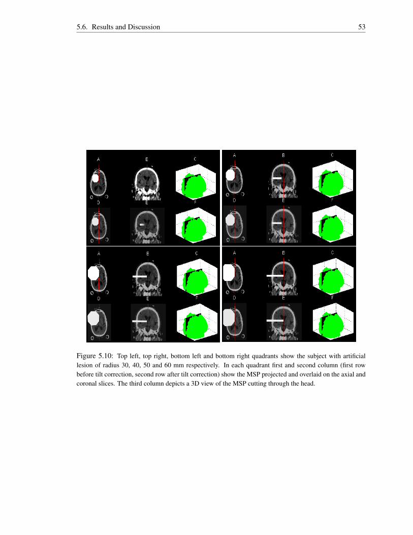
5.6. Results and Discussion 53
Figure 5.10: Top left, top right, bottom left and bottom right quadrants show the subject with artificiallesion of radius 30, 40, 50 and 60 mm respectively. In each quadrant first and second column (first rowbefore tilt correction, second row after tilt correction) show the MSP projected and overlaid on the axial andcoronal slices. The third column depicts a 3D view of the MSP cutting through the head.
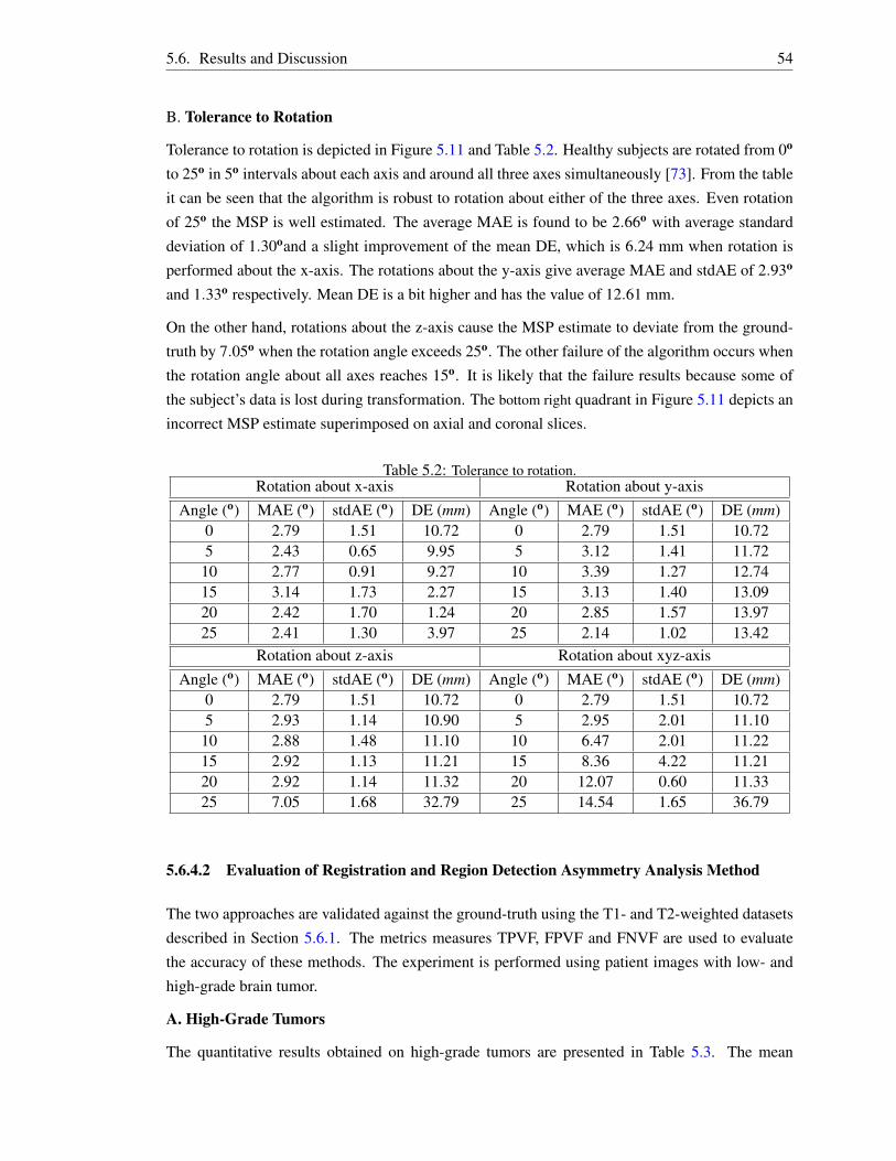
5.6. Results and Discussion 54
B. Tolerance to Rotation
Tolerance to rotation is depicted in Figure 5.11 and Table 5.2. Healthy subjects are rotated from 0o
to 25o in 5o intervals about each axis and around all three axes simultaneously [73]. From the table
it can be seen that the algorithm is robust to rotation about either of the three axes. Even rotation
of 25o the MSP is well estimated. The average MAE is found to be 2.66o with average standard
deviation of 1.30oand a slight improvement of the mean DE, which is 6.24 mm when rotation is
performed about the x-axis. The rotations about the y-axis give average MAE and stdAE of 2.93o
and 1.33o respectively. Mean DE is a bit higher and has the value of 12.61 mm.
On the other hand, rotations about the z-axis cause the MSP estimate to deviate from the ground-
truth by 7.05o when the rotation angle exceeds 25o. The other failure of the algorithm occurs when
the rotation angle about all axes reaches 15o. It is likely that the failure results because some of
the subject’s data is lost during transformation. The bottom right quadrant in Figure 5.11 depicts an
incorrect MSP estimate superimposed on axial and coronal slices.
Table 5.2: Tolerance to rotation.Rotation about x-axis Rotation about y-axis
Angle (o) MAE (o) stdAE (o) DE (mm) Angle (o) MAE (o) stdAE (o) DE (mm)0 2.79 1.51 10.72 0 2.79 1.51 10.725 2.43 0.65 9.95 5 3.12 1.41 11.7210 2.77 0.91 9.27 10 3.39 1.27 12.7415 3.14 1.73 2.27 15 3.13 1.40 13.0920 2.42 1.70 1.24 20 2.85 1.57 13.9725 2.41 1.30 3.97 25 2.14 1.02 13.42
Rotation about z-axis Rotation about xyz-axisAngle (o) MAE (o) stdAE (o) DE (mm) Angle (o) MAE (o) stdAE (o) DE (mm)
0 2.79 1.51 10.72 0 2.79 1.51 10.725 2.93 1.14 10.90 5 2.95 2.01 11.1010 2.88 1.48 11.10 10 6.47 2.01 11.2215 2.92 1.13 11.21 15 8.36 4.22 11.2120 2.92 1.14 11.32 20 12.07 0.60 11.3325 7.05 1.68 32.79 25 14.54 1.65 36.79
5.6.4.2 Evaluation of Registration and Region Detection Asymmetry Analysis Method
The two approaches are validated against the ground-truth using the T1- and T2-weighted datasets
described in Section 5.6.1. The metrics measures TPVF, FPVF and FNVF are used to evaluate
the accuracy of these methods. The experiment is performed using patient images with low- and
high-grade brain tumor.
A. High-Grade Tumors
The quantitative results obtained on high-grade tumors are presented in Table 5.3. The mean
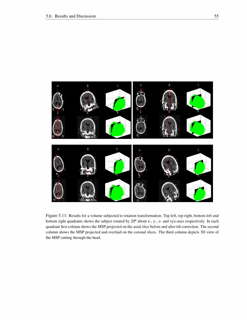
5.6. Results and Discussion 55
Figure 5.11: Results for a volume subjected to rotation transformation. Top left, top right, bottom left andbottom right quadrants shows the subject rotated by 20o about x-, y-, z- and xyz-axes respectively. In eachquadrant first column shows the MSP projected on the axial slice before and after tilt correction. The secondcolumn shows the MSP projected and overlaid on the coronal slices. The third column depicts 3D view ofthe MSP cutting through the head.
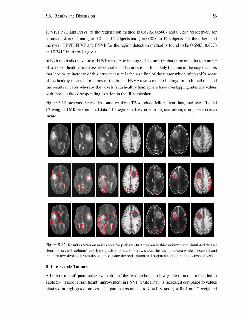
5.6. Results and Discussion 56
TPVF, FPVF and FNVF of the registration method is 0.6793, 0.8607 and 0.3207 respectively for
parameter λ = 0.7, and ζ = 0.01 on T2 subjects and ζ = 0.005 on T1 subjects. On the other hand
the mean TPVF, FPVF and FNVF for the region detection method is found to be 0.6583, 0.6773
and 0.3417 in the order given.
In both methods the value of FPVF appears to be large. This implies that there are a large number
of voxels of healthy brain tissues classified as brain lesions. It is likely that one of the major factors
that lead to an increase of this error measure is the swelling of the tumor which often shifts some
of the healthy internal structures of the brain. FNVF also seems to be large in both methods and
this results in cases whereby the voxels from healthy hemisphere have overlapping intensity values
with those at the corresponding location in the ill hemisphere.
Figure 5.12 presents the results found on three T2-weighted MR patient data, and two T1- and
T2-weighted MR on simulated data. The segmented asymmetric regions are superimposed on each
image.
Figure 5.12: Results shown on axial slices for patients (first column to third column) and simulated dataset(fourth to seventh column) with high-grade gliomas. First row shows the raw input data while the second andthe third row depicts the results obtained using the registration and region detection methods respectively.
B. Low-Grade Tumors
All the results of quantitative evaluation of the two methods on low-grade tumors are detailed in
Table 5.4. There is significant improvement in FNVF while FPVF is increased compared to values
obtained in high-grade tumors. The parameters are set to λ = 0.8, and ζ = 0.01 on T2-weighted
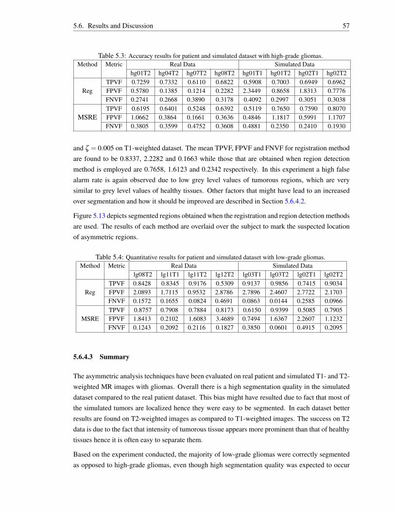
5.6. Results and Discussion 57
Table 5.3: Accuracy results for patient and simulated dataset with high-grade gliomas.Method Metric Real Data Simulated Data
hg01T2 hg04T2 hg07T2 hg08T2 hg01T1 hg01T2 hg02T1 hg02T2
RegTPVF 0.7259 0.7332 0.6110 0.6822 0.5908 0.7003 0.6949 0.6962FPVF 0.5780 0.1385 0.1214 0.2282 2.3449 0.8658 1.8313 0.7776FNVF 0.2741 0.2668 0.3890 0.3178 0.4092 0.2997 0.3051 0.3038
MSRETPVF 0.6195 0.6401 0.5248 0.6392 0.5119 0.7650 0.7590 0.8070FPVF 1.0662 0.3864 0.1661 0.3636 0.4846 1.1817 0.5991 1.1707FNVF 0.3805 0.3599 0.4752 0.3608 0.4881 0.2350 0.2410 0.1930
and ζ = 0.005 on T1-weighted dataset. The mean TPVF, FPVF and FNVF for registration method
are found to be 0.8337, 2.2282 and 0.1663 while those that are obtained when region detection
method is employed are 0.7658, 1.6123 and 0.2342 respectively. In this experiment a high false
alarm rate is again observed due to low grey level values of tumorous regions, which are very
similar to grey level values of healthy tissues. Other factors that might have lead to an increased
over segmentation and how it should be improved are described in Section 5.6.4.2.
Figure 5.13 depicts segmented regions obtained when the registration and region detection methods
are used. The results of each method are overlaid over the subject to mark the suspected location
of asymmetric regions.
Table 5.4: Quantitative results for patient and simulated dataset with low-grade gliomas.Method Metric Real Data Simulated Data
lg08T2 lg11T1 lg11T2 lg12T2 lg03T1 lg03T2 lg02T1 lg02T2
RegTPVF 0.8428 0.8345 0.9176 0.5309 0.9137 0.9856 0.7415 0.9034FPVF 2.0893 1.7115 0.9532 2.8786 2.7896 2.4607 2.7722 2.1703FNVF 0.1572 0.1655 0.0824 0.4691 0.0863 0.0144 0.2585 0.0966
MSRETPVF 0.8757 0.7908 0.7884 0.8173 0.6150 0.9399 0.5085 0.7905FPVF 1.8413 0.2102 1.6083 3.4689 0.7494 1.6367 2.2607 1.1232FNVF 0.1243 0.2092 0.2116 0.1827 0.3850 0.0601 0.4915 0.2095
5.6.4.3 Summary
The asymmetric analysis techniques have been evaluated on real patient and simulated T1- and T2-
weighted MR images with gliomas. Overall there is a high segmentation quality in the simulated
dataset compared to the real patient dataset. This bias might have resulted due to fact that most of
the simulated tumors are localized hence they were easy to be segmented. In each dataset better
results are found on T2-weighted images as compared to T1-weighted images. The success on T2
data is due to the fact that intensity of tumorous tissue appears more prominent than that of healthy
tissues hence it is often easy to separate them.
Based on the experiment conducted, the majority of low-grade gliomas were correctly segmented
as opposed to high-grade gliomas, even though high segmentation quality was expected to occur
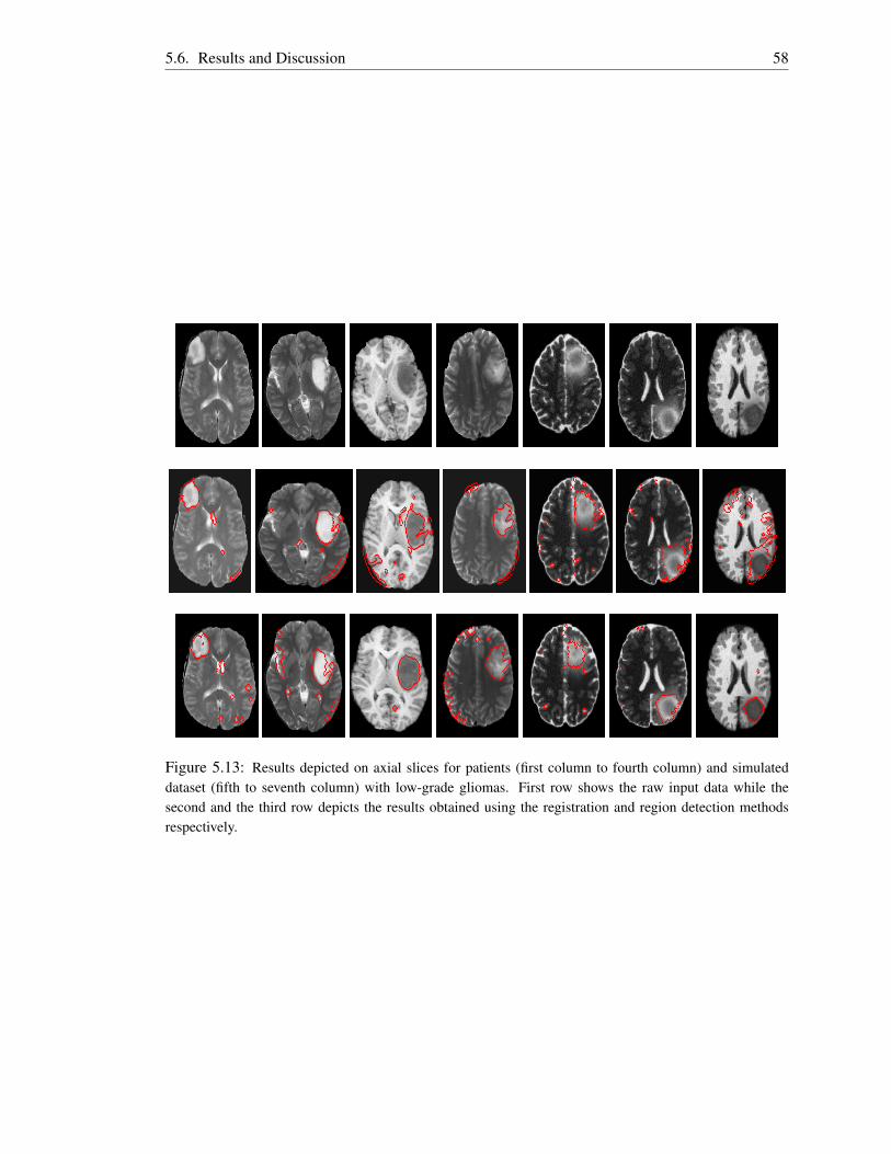
5.6. Results and Discussion 58
Figure 5.13: Results depicted on axial slices for patients (first column to fourth column) and simulateddataset (fifth to seventh column) with low-grade gliomas. First row shows the raw input data while thesecond and the third row depicts the results obtained using the registration and region detection methodsrespectively.

5.6. Results and Discussion 59
on high-grade gliomas. The major contributing factor to this bias could be the difference in patient
dataset used as most of high-grade gliomas are large in size and often have overlapping intensity
distribution with brain ventricles. In some datasets the symmetry plane passes through the tumor
and this makes small portions of the tumor on the other hemisphere to appear symmetric over the
plane.
For most of the experiments done, the registration-based method achieved a higher TPVF than
the region detection-based method. This simply means that a large number of tumor voxels are
correctly classified with the registration-based method. However, the value of FPVF is also large
which signals that this technique is likely to classify healthy brain tissues as brain tumors.
The parameter values for λ and ζ are systematically changed to obtain a good tumor segmentation
based on the image modality and the type of tumors to be segmented. For both high-grade and
low-grade gliomas, when the value of λ is increased the number of false tumor voxels increases
faster than the number of correct ones. Hence the fraction of false detection increases notably on
high-grade tumors. On the other hand, reducing the value of λ drops the percentage of correct
classification as many of the lesion’s voxels are missed, especially on low-grade gliomas. For this
reason the value of λ is set a bit larger on low-grade gliomas than on high-grade lesions. The
parameter ζ is set to a small value on patient images with low-grade gliomas since lesions of this
type appear with low grey level voxel values which sometimes overlap with other healthy brain
structures. On patient datasets with high-grade gliomas ζ is set to a larger value to reduce the error
of classifying healthy brain tissues.
Chapter 6
Atlas-Based Pathology Detection
This chapter presents a knowledge-based method used to develop a model of healthy brain tissues.
This model is further used to detect abnormal tissues in future medical scans. The knowledge
is represented in the form of brain atlas constructed from a set of healthy medical images. The
same principles applied in [6] are adopted with some improvements on the procedure used for atlas
construction. Functionality for incorporating partial datasets into the atlas space has been added.
The outline of this chapter is as follows. Section 6.1 describes the approach followed in construct-
ing the atlas. In Section 6.2 a detailed description to detect pathological tissues is given while
Section 6.3 describes methods used to remove false positives. The chapter concludes with results
and discussion in Section 6.4.
6.1 Building Atlas
The method presented in [6] follows a single pass approach to construct the atlas. The drawback of
this approach is that it does not necessarily minimize the error between the atlas and the remaining
set of images. Hence it does not perform some optimizations needed to generate a high quality
atlas. To address this weakness the atlas construction method is formulated as an optimization
problem which minimizes the sum of square difference between the current atlas estimate and a
reference image. This technique is inspired by the popular shape alignment approach, generalized
Procrustes analysis (GPA), which aligns shapes with corresponding numbers of points so that the
sum of the distance of each shape to the mean is minimized [74].
6.1.1 Generalized Procrustes Analysis (GPA)
This is an iterative technique used to align shapes onto the same shape-coordinate space such that
the square error distance between each shape to the mean shape is minimized [74]. In this work the
60
6.1. Building Atlas 61
same method is adopted with the objects of interest to be aligned being brain scans having different
sizes and orientations. The algorithm converges if the SSD between the reference image and mean
image is less than some predefined threshold.
6.1.1.1 Choosing Initial Reference
The initial reference image is chosen manually from the existing set of images through inspection
that it best represents the average population [75]. The arbitrarily chosen reference image is likely
to bias the atlas to a specific patient especially if the patient scan is not within the average popula-
tion the atlas is was constructed for [75]. This image defines the estimate of the coordinate space
onto which the entire set of images will be mapped. All the images have the same dimensions
with voxels of cubic millimeter in size. After aligning these images the atlas is constructed, which
consists of mean and maximum variance of the intensity and displacement field for each voxel [6].
Maximum variance of the intensity and displacement fields define the grey level and deformation
field thresholds on every voxel.
6.1.1.2 Image Alignment
Given a reference image R a group-wise image registration is applied to map each image (F1, ...,FN)
to a single coordinate frame defined by R. The registration process is performed in two steps. At
first affine transformations are applied to the rest of the images to globally match the reference
image. For each image Fi a transformation Ti, which minimizes the similarity measure between
Fi and R, has to be found to map Fi onto R. After performing a global alignment between the
two images, a nonrigid registration [43] is applied to remove local deformations which might have
occurred because of differences in shape of internal brain structures. A multiresolution technique
is adopted during registration to improve the performance.
When performing affine registration SSD is used as the similarity measure to be minimized be-
tween the two images. SSD is used since the images to be aligned are of the same modality and
it is easy to compute. Also it can be optimized easily using the LM method. The mathematical
formulation of this similarity measure is defined as
SSD(u) =12
Nx
∑x=1
Ny
∑y=1
Nz
∑z=1
[Fi(Ti(x : u))−R(x)]2 , (6.1)
where x = (x,y,z), Ti(x : u) represents a 9-parameter affine transformation and u = [θ , β , φ , Tx,
Ty, Tz, Sx, Sy, Sz]T is the parameter vector used to define the transformation. A literature on medical
image registration is discussed in Chapter 3. A homogeneous coordinates is used in this case and
the affine transformation is represented by a 4×4 matrix [44]. The transformation consists of three
rotational angles, translation and scale parameters along the three axes and can be written as

6.1. Building Atlas 62
Ti(u) = TlRxRyRzS, (6.2)
where
Tl =
1 0 0 Tx
0 1 0 Ty
0 0 1 Tz
0 0 0 1
, S =
Sx 0 0 0
0 Sy 0 0
0 0 Sz 0
0 0 0 1
,
Ry =
cosβ 0 sinβ 0
0 1 0 0
−sinβ 0 cosβ 0
0 0 0 1
, Rz =
cosφ −sinφ 0 0
sinφ cosφ 0 0
0 0 1 0
0 0 0 1
,
Rx =
1 0 0 0
0 cosθ −sinθ 0
0 sinθ cosθ 0
0 0 0 1
.
(6.3)
The optimal value of u is determined by an iterative optimization method. The LM method is used
in this work because of its mechanism of switching back and forth between GD and GN, hence
acquiring the capabilities of the two methods such as stability and convergence speed [44, 51, 53].
In summary the general flow for finding u follows the same principles applied in Section 5.2.6
when searching for the optimal value of the plane parameter vector. The changes that have been
made are the use of Ti instead of the reflection transformation TRF and an increase of the number
of optimization parameters in u from four to nine. This transformation is applied on Fi to generate
a new image Fui . Numerical differentiation of Fu
i is computed to estimate the Jacobian Matrix J(u)of size 9×NxNyNz. The search direction dk is calculated after diagonal elements of the Hessian
matrix estimate (JT (u)J(u)) are augmented with a damping factor µ . Values of both µ and δ are
set and updated as detailed in Section 5.2.6. Multi-resolution is also adopted in this case and only
the translation parameters are modified after the convergence is reached at the coarser level.
Even though Fi globally maps to R after the affine transformation is applied, this does not necessar-
ily mean that the internal structures of the brain scans match one another. Hence local registration
has to be applied to remove these local differences. The nonrigid registration toolbox MIRT, pre-
sented in [43] is employed at this stage.

6.1. Building Atlas 63
6.1.1.3 Procrustes Distance (PD)
The Procrustes distance is a measure of the sum of the distances between corresponding points
of two shapes. It evaluates how close one shape is to another. Hence the lower the value is the
closer the two shapes are. In this thesis PD is computed as the sum of squared intensity difference
between corresponding voxels of two volumes. Given a reference volume R and the mean intensity
volume MI , the PD is computed as shown below:
PD =12
Nx
∑x=1
Ny
∑y=1
Nz
∑z=1
[R(x,y,z)−MI(x,y,z)]2 , (6.4)
where Nx×Ny×Nz is the size of each volume.
6.1.2 Atlas Construction
Given a set of normal brain images that have been correctly mapped onto one coordinate space,
the mean and maximum variance volumes are computed to represent the brain atlas. The mean in-
tensity (MI) and mean displacement (MV ) volume define the expected grey level and displacement
fields of each voxel respectively. They are calculated by averaging the intensity and deformation
field norm of the aligned images as
MI =1N ∑
Ni=1 Fi, MV = 1
N ∑Ni=1 Vi, (6.5)
where N is the total number of aligned volumes, Fi = Fi(Ti(x : u)) is the registered image, Vi is the
magnitude of the displacement field, while subscripts I and V represent intensity and displacement
field respectively. Maximum variance intensity (VI) and maximum variance displacement field
(VV ) volume define for each voxel a threshold value for which the voxel intensity and displacement
is expected to deviate from MI and MV respectively for it to be considered normal. Maximum
variance intensity is computed by calculating the variance of each aligned volume and retaining
the voxels with a high confidence grey level difference. Also maximum variance displacement
field defines voxels with a high confidence shift difference from MV . These can be represented
mathematically as
VI(x,y,z) = argmax1≤i≤N
{[Fi(x,y,z)−MI(x,y,z)]
2},
VV (x,y,z) = argmax1≤i≤N
{[Vi(x,y,z)−MV (x,y,z)]
2},
(6.6)
where 1 ≤ x ≤ Nx, 1 ≤ y ≤ Ny and 1 ≤ z ≤ Nz. In summary the algorithm involves the following
steps to create a brain atlas from the set of healthy brain images.

6.2. Abnormal Tissue Detection 64
Input: (set of brain scans in axial format (F1,F2,F3, ...,FN), stopping criterion [ε0])
Output: (mean and maximum variance of intensity and displacement volume (MI,VI,MV ,VV ))
Algorithm
Begin
Step 0: Manually select the reference volume R.
Step 1: Perform rigid and nonrigid registration to align each image Fi onto R.
Step 2: Compute mean volume MI from aligned images.
Step 3: Calculate SSD between MI and R. if SSD < ε0 goto Step 5.
Step 4: Update reference volume with mean volume, R = MI , goto Step 1.
Step 5: Compute maximum variance intensity volume VI , MV and VV .
End
Figure 6.1 shows the axial, sagittal and coronal view slices of the constructed atlas. The atlas is
built using healthy simulated T1-weighted brain MR images. The bright regions in intensity and
deformation field variance mark voxels expected to have large intensity and displacement field
variations respectively.
6.2 Abnormal Tissue Detection
In this section details of two different approaches followed to detect abnormal tissues are given.
They follow the same principles used when constructing the brain atlas. The differences between
these methods are a consequence of differences in the dataset to be handled. The first technique
detects abnormalities on a full scanned volume while the second method detects abnormal masses
on partial scans. A dataset is declared partial if the volume does not contain the entire brain. For
example the volume may only cover the information from the brain-stem to the corpus callosum or
from the corpus callosum to the scalp.
6.2.1 Abnormality Detection on Full Scans
The main objective of an abnormal tissue detection algorithm is to produce a binary volume Lthat estimates the proposed location of tumorous tissues in the brain. These tissues have intensity
values that deviate from the expected values MI of a healthy brain. To detect these tissues a two
stage technique which follows the same principles used to construct the atlas is proposed.
The initial step is to align patient volume F with the atlas template MI . The alignment is achieved
by dividing the registration process into two steps. Firstly, a global registration is performed using

6.2. Abnormal Tissue Detection 65
Figure 6.1: Brain atlas in T1-weighted MR images acts as the model of healthy brain tissues. From top tobottom: axial, coronal and sagittal view of the atlas. From left to right: expected grey level, maximum in-tensity variance, expected norm of the displacement field, and maximum variance norm of the displacementfield for each voxel.

6.2. Abnormal Tissue Detection 66
a 9-parameter affine transformation with SSD as the similarity measure to bring the two volumes
into global correspondence. Secondly, a nonrigid registration is applied to compensate for the
morphological differences between internal structures of the brain, with large deformation expected
to arise on the regions that have been deformed by the tumor. The deformation magnitude of each
voxel is defined in a volume U.
After the alignment, the intensity square difference between the atlas and the registered patient
volume is calculated for each voxel. This value defines the amount by which a voxel deviates from
its expected grey level value. Also, the deformation field difference between the atlas mean and
test image displacement field is computed to determine the displacement variance of each voxel. A
voxel is declared abnormal if its intensity square difference is greater than its maximum variance
intensity or its displacement square difference is greater than its maximum variance deformation
norm. Mathematically this is represented by the following function:
L(x,y,z) =
1 ,MV (x,y,z)< DI(x,y,z) or VV (x,y,z)< DV (x,y,z)
0 ,Otherwise,(6.7)
where DI(x,y,z) =[MI(x,y,z)− F̄(x,y,z)
]2 is the square difference between atlas mean the MI
and a registered patient volume F̄, and DV (x,y,z) = [MV (x,y,z)−U(x,y,z)]2. Figure 6.2 shows
intermediate results for detecting voxels having intensity values and deformation field larger or
smaller than expected.
6.2.2 Abnormality Detection on Partial Scans
Given a partial scan P the main idea is to align P onto the the atlas space so that analysis can be
performed to determine anomalies. Aligning partial scans becomes a challenging task since there
are data missing from P. Hence in order to bring P into global correspondence with the atlas, a
tranformation T is estimated from 2D transformations using mid-sagittal and coronal slices of both
P and MI . This is done firstly by defining a new volume Q which has the same dimensions as MI .
P is then embedded into Q such that the center of grid volume of P maps exactly with the center
of grid volume of Q. The MSP in Q is extracted using the method described in Section 5.2, which
is then used to remove tilting and rotation such that mid-sagittal slice passes through the center of
the grid volume.
Normally MSP is used to determine the rotation transformations about the y-axis and z-axis but it
is still a challenging problem to estimate the rotation transformation about x-axis. To determine
the transformation automatically, one of the options is to find two of the eight Talairach point
landmarks: the anterior commissure (AC) and the posterior commissure (PC) located on the mid-
sagittal slice [76, 20]. AC and AP are then joined by a straight line and the angle which this line
makes with the XY plane marks the rotation angle about x-axis. A drawback of this approach is

6.2. Abnormal Tissue Detection 67
Figure 6.2: Intermediate results for atlas-based tumor detection method. Top row from left to right: meanintensity (MI), maximum intensity variance (MV ), test image before registration (F), deformed test imageafter registration (F̄), the intensity square difference (DI) between (VI) and (F̄), binary image where (DI >
VI). Bottom row from left to right: mean displacement field (MV ), maximum variance of the displacementfield (VV ), the deformation field norm (U) of the registered test image, displacement field square difference(DV ) between (MV ) and (U), binary image where (DV > VV ). The binary images mark the suspectedlocation of the anomalies.
that AC and AP are visible only in MR images and are manually annotated.
A general method to estimate the transformation about x-axis is based on the assumption that both
MI and Q are of the same modality. Firstly, 2D mid-sagittal slices SM and SQ are extracted from
MI and Q respectively. A 2D affine transformation about the x-axis (T2x) which maps SQ onto SM
is then obtained by minimizing the SSD between the two slices. The transformation is formulated
into a 4× 4 affine transformation T3x, since homogeneous coordinates are used, and applied to
Q to generate a new volume Qx which has the same number of coronal slices with those of MI .
Secondly, two arbitrary coronal slices, CM and CQ at the same level are chosen from MI and Qx in
the order given. These slices are used to obtain a 2D affine transformation T2y which aligns CQ onto
CM which is also formulated into a 4×4 matrix T3y. In reality if Qx was to be transformed using
T3y that would have subjected Q to large degradation due to multiple interpolation. Hence, instead
of applying T3y to Qx, a better solution is to combine T3x and T3y to form a single transformation
T = T3yT3x which globally aligns Q onto MI .
A nonrigid registration stage is performed to compensate for local displacement, with large de-
formation expected to occur in regions which have been severely damaged by brain tumors. The
registration is applied on the volume containing the partial data by omitting some slices in MI
which correspond to empty slices in Q. After the alignment is achieved the square difference
between the two partial volumes is computed and abnormal voxels are declared as described in
Section 6.2.1.
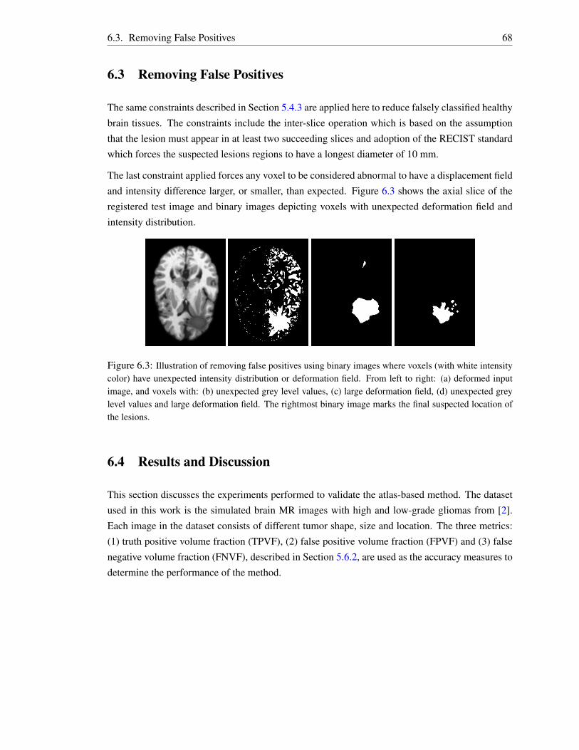
6.3. Removing False Positives 68
6.3 Removing False Positives
The same constraints described in Section 5.4.3 are applied here to reduce falsely classified healthy
brain tissues. The constraints include the inter-slice operation which is based on the assumption
that the lesion must appear in at least two succeeding slices and adoption of the RECIST standard
which forces the suspected lesions regions to have a longest diameter of 10 mm.
The last constraint applied forces any voxel to be considered abnormal to have a displacement field
and intensity difference larger, or smaller, than expected. Figure 6.3 shows the axial slice of the
registered test image and binary images depicting voxels with unexpected deformation field and
intensity distribution.
Figure 6.3: Illustration of removing false positives using binary images where voxels (with white intensitycolor) have unexpected intensity distribution or deformation field. From left to right: (a) deformed inputimage, and voxels with: (b) unexpected grey level values, (c) large deformation field, (d) unexpected greylevel values and large deformation field. The rightmost binary image marks the final suspected location ofthe lesions.
6.4 Results and Discussion
This section discusses the experiments performed to validate the atlas-based method. The dataset
used in this work is the simulated brain MR images with high and low-grade gliomas from [2].
Each image in the dataset consists of different tumor shape, size and location. The three metrics:
(1) truth positive volume fraction (TPVF), (2) false positive volume fraction (FPVF) and (3) false
negative volume fraction (FNVF), described in Section 5.6.2, are used as the accuracy measures to
determine the performance of the method.

6.4. Results and Discussion 69
6.4.1 Evaluation on Full Scan
A. High-Grade Tumor
Figure 6.4 illustrates the suspected locations of the lesions in each test image. These regions mark
voxels with intensity and deformation field norm larger or smaller than the expected values. In
some images, such as the third image in the bottom row of Figure 6.4, the suspected abnormal
region covers the healthy regions surrounding them.
The quantitative results of the method on high-grade gliomas are shown in Table 6.1. The average
TPVF, FPVF and FNVF are found to be 0.6501, 0.8971 and 0.3499 respectively. Though the
bottom row of Figure 6.4 shows axials with tumors entirely covered, the algorithm did not detect
abnormal voxels in other axial slices hence the reason why FNVF is high. The value of FPVF are
found to be large and this indicates that the method misclassifies a large number of healthy tissue
subjects. It is likely that the major contributing factor is the large deformation occurring around
lesions because of the minimization of the cost function by the nonrigid registration process.
Figure 6.4: The results for atlas-based method depicted on axial slice for simulated dataset with high-gradegliomas. First row: raw input data, second row: deformed test image with suspected location (red contour)overlaid on each image.
B. Low-Grade Tumor
The performance of the method is also evaluated on low-grade gliomas. Figure 6.5 illustrates visual
results for six T1-weighted MR images. In each dataset the visual results are shown in axial view
by selecting an abitrary axial slice containing the tumor. Table 6.2 shows quantitative results on
these dataset. The mean TPVF, FPVF and FNVF of the proposed method on low-grade gliomas
are 0.7132, 1.9565 and 0.2868 in the order given. The value of FPVF being larger than 1 implies
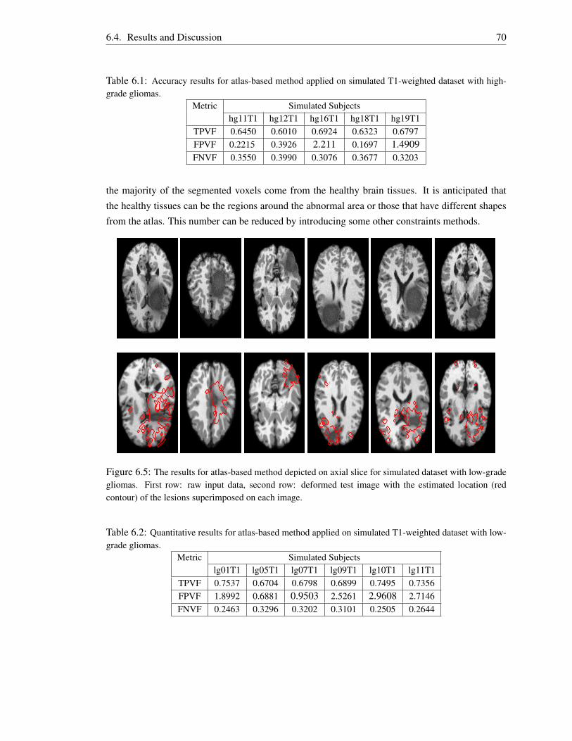
6.4. Results and Discussion 70
Table 6.1: Accuracy results for atlas-based method applied on simulated T1-weighted dataset with high-grade gliomas.
Metric Simulated Subjectshg11T1 hg12T1 hg16T1 hg18T1 hg19T1
TPVF 0.6450 0.6010 0.6924 0.6323 0.6797FPVF 0.2215 0.3926 2.211 0.1697 1.4909FNVF 0.3550 0.3990 0.3076 0.3677 0.3203
the majority of the segmented voxels come from the healthy brain tissues. It is anticipated that
the healthy tissues can be the regions around the abnormal area or those that have different shapes
from the atlas. This number can be reduced by introducing some other constraints methods.
Figure 6.5: The results for atlas-based method depicted on axial slice for simulated dataset with low-gradegliomas. First row: raw input data, second row: deformed test image with the estimated location (redcontour) of the lesions superimposed on each image.
Table 6.2: Quantitative results for atlas-based method applied on simulated T1-weighted dataset with low-grade gliomas.
Metric Simulated Subjectslg01T1 lg05T1 lg07T1 lg09T1 lg10T1 lg11T1
TPVF 0.7537 0.6704 0.6798 0.6899 0.7495 0.7356FPVF 1.8992 0.6881 0.9503 2.5261 2.9608 2.7146FNVF 0.2463 0.3296 0.3202 0.3101 0.2505 0.2644

6.4. Results and Discussion 71
6.4.2 Summary
The work presented here showed that a brain atlas can be used to estimate a model of healthy
brain tissues and can further be utilized to accurately detect and segment brain lesions in future
images. The atlas was constructed from scratch using a set of healthy T1-weighted MR images
and the proposed method, which is fully automated, was evaluated on high-grade and low-grade
gliomas. To determine the performance of the method its accuracy is compared to that of the gold-
standard technique, manual segmentation, and it gives reasonable results. A detailed description of
the approaches employed to remove non-tumorous voxels was also given.
In summary TPVF and FPVF are found to be 0.6501 and 0.8971 on high-grade gliomas and 0.7132,
and 1.9565 on low-grade gliomas. A large value of FPVF means most of the voxels classified as
brain lesions come from the healthy brain tissues. Hence over segmentation is performed. This
is caused by large displacement of healthy brain tissues surrounding the lesions which are left out
during manual segmentation. Since this is an error, a constraint which takes into consideration the
intensity distribution and displacement field of the surrounding tissues was applied to reduce it.

Chapter 7
Conclusion
The main objective of this thesis was to develop an automatic CAD method which is able to detect
and segment brain abnormalities in 3D MR and CT data accurately. Two automatic methods have
been developed. The first method is based on the analysis of the symmetry of the brain, and has
been tested and evaluated on T1- and T2-weighted MR datasets. The second method, based on
the expected intensity values of healthy brain tissues, has been evaluated on T1-weighted MR
dataset. In this chapter the discussed techniques are reviewed and the limitations, and possible
future improvements, on each method are suggested.
7.1 Summary of this Thesis
The proposed symmetry-based method consists of three steps: detection of the symmetry, tilt cor-
rection and asymmetry quantification. The symmetry detection method starts first by isotropically
resampling the MR dataset to cubic voxels to avoid the influence of the slice thickness on the vol-
ume of small-sized tissues. It then estimates the parameters of the symmetry plane by formulating
the task as a registration problem and adopts Levenberg-Marquardt as the optimization algorithm.
The obtained optimal parameter values are then compared to ground-truth using two accuracy mea-
sures: MAE and DE. The plane is further used to correct tilting of the head such that it becomes
upright.
Having found the symmetry plane the algorithm continues to analyze the symmetry of the brain to
segment out asymmetric regions, suspected to be brain abnormalities. Two automatic approaches
have been developed to quantify asymmetric regions. They are based on the assumption that the
brain shows a bilateral symmetry and this symmetry is only violated if the patient is suffering from
brain lesions. The first method analyzes the voxel intensity difference between brain hemispheres,
with large absolute difference expected to appear in regions which are asymmetric. The second
approach is based on a 2D region detector. They are further compared to the ground-truth using
TPVF, FPVF and FNVF as accuracy measures and the results obtained show that it is possible to
72

7.2. Limitations and Future Work 73
estimate the location of brain tumors using asymmetry.
The experiments showed that the registration method was more accurate than the region detector
based method though at the cost of a high false negative rate and computational costs. Both ex-
periments were performed on a personal computer. The total run time, per 256×256×181 cubic
voxel volume, for the registration-based method is 26.17±2.34 minutes and 9.616±1.30 minutes
for the region detection-based method. A good estimate of the symmetry plane is achieved with a
run time of 4.81±1.50 minutes.
An atlas-based brain tumor segmentation method was also studied in this work, using voxel in-
tensities and displacement fields as the prior knowledge of healthy brain tissues. The atlas was
constructed from a set of healthy simulated T1-weighted MR images adopting GPA to align differ-
ent subjects onto the same coordinate space. The atlas consists of the expected intensity value and
displacement field for each voxel. It also has threshold values (intensity and displacement field)
for each voxel which are set automatically from the healthy subjects.
The experiments were performed using simulated subjects with artificial abnormalities and the
segmented regions were compared with the ground-truth using TPVF, FPVF and FNVF as accu-
racy measures. Promising results were obtained though at the cost of higher false positive rates.
Different subjects having different types of tumors were tested and the results on each type were
discussed. The overall computational time was 31.42± 4.3 minutes per 256× 256× 181 cubic
voxel volume, and is affected by the nonrigid registration process and the presence of a large num-
ber of false positives to be removed.
7.2 Limitations and Future Work
The major limitation of the symmetry-based method is inability to handle large symmetric lesions
which crosses the symmetry line, or a pair of symmetric lesions. These challenges still remains as
obstacles in the work in the literature. For the case where the pair of lesions have different sizes
or lesions crossing the symmetry line do not occur symmetrically on both hemispheres [10] have
added the functionality of the region growing techniques to address this issues. The seed points
are selected automatically from the remaining asymmetric fractions after computing the intensity
difference between the hemispheres to cancel out symmetrical portions.
The other remaining challenge is the issue of a large number of false positives, in both methods,
despite the number of constraints which were enforced. Future work will be to investigate other
possible methods to reduce the falsely-classified healthy tissues.

Bibliography
[1] Michael R. Kaus, Simon K. Warfield, Arya Nabavi, Peter M. Black, Ferenc A. Jolesz, and
Ron Kikinis. Automated segmentation of brain tumors. MRI datasets were last accessed
on 2013-10-08 from http://spl.harvard.edu/publications/bitstream/download/
5270.
[2] B. Menze, A. Jakab, S. Bauer, M. Reyes, M. Prastawa, and K. Van Leemput. Multi-
modal brain tumor segmentation. Accessed on 2013-10-08 from: http://www.imm.dtu.
dk/projects/BRATS2012.
[3] Yujun Guo. Medical image registration and application to atlas-based segmentation. PhD
thesis, Kent State University, 2007.
[4] Raymond Y. Kwong and E. Kent Yucel. Computed tomography scan and magnetic resonance
imaging. Circulation, 108(15):104–106, 2003.
[5] Bassem A. Abdullah. Segmentation of Multiple Sclerosis Lesions in Brain MRI. PhD thesis,
University of Miami, 2012.
[6] Jean Francois Laliberte, Jean Meunier, Max Mignotte, and Jean Paul Soucy. Detection of
diffuse abnormal perfusion in SPECT using a normal brain atlas. NeuroImage, 23(2):561 –
568, 2004.
[7] L. Manoj, M. Kalyani, K. Jyothi, G. Ganga Bhavani, and V. Govardhani. Review of brain and
brain cancer treatment. International Journal of Pharma and Bio Sciences, 2:468–477, 2011.
[8] Brain tumors in radiation oncology. Radiation Oncology , Box 356043, 1959
N.E. Pacific St. Seattle, WA 98195 , 206-598-4100, October 2006. Available
(online) from: https://healthonline.washington.edu/document/health_online/
pdf/Brain_Tumors_10_06.pdf.
[9] Shantanu Banik, Rangaraj M. Rangayyan, and Graham S. Boag. Landmarking and segmen-
tation of 3D CT images. Morgan and Claypool Publishers, 2009.
[10] Xin Liu. Asymmetry Analysis and its Significance in Neuro-Imaging Applications. PhD thesis,
Columbia University, New York, NY, USA, 2008.
74

Bibliography 75
[11] M.C. Clark, L.O. Hall, D.B. Goldgof, R. Velthuizen, F.R. Murtagh, and M.S. Silbiger. Auto-
matic tumor segmentation using knowledge-based techniques. IEEE Transactions on Medical
Imaging, 17(2):187–201, 1998.
[12] Sonali Patil and V.R. Udupi. A computer aided diagnostic system for classification of brain
tumors using texture features and probabilistic neural network. IJCSEITR, 3:61–66, 2013.
[13] D. Cherifi, M.Z. Doghmane, A. Nait-Ali, Z. Aici, and S. Bouzelha. Abnormal tissues ex-
traction in MRI brain medical images. In Systems, Signal Processing and their Applications
(WOSSPA), 2011 7th International Workshop on. IEEE, 2011.
[14] Mehdi Jafari and Shohreh Kasaei. Automatic brain tissue detection in MRI images using
seeded region growing segmentation and neural network classification. Australian Journal of
Basic and Applied Sciences, 5(8):1066–1079, 2011.
[15] N.E.A. Khalid, S. Ibrahim, and P.N.M.M. Haniff. MRI brain abnormalities segmentation
using K-Nearest Neighbors (k-NN). International Journal on Computer Science and Engi-
neering (IJCSE), 3(2), February 2011.
[16] Lei Wang, Li Liu, and Latifur Khan. Automatic image annotation and retrieval using subspace
clustering algorithm. In Proceedings of the 2Nd ACM International Workshop on Multimedia
Databases, MMDB ’04, 100–108, New York, NY, USA, 2004. ACM.
[17] Nursuriati Jamil and Siti’Aisyah Sa’adan. Automatic image annotation using color k-means
clustering. In Halimah Badioze Zaman, Peter Robinson, Maria Petrou, Patrick Olivier, Heiko
Schröder, and Timothy K. Shih, editors, Visual Informatics: Bridging Research and Practice,
volume 5857 of Lecture Notes in Computer Science, 645-652. Springer Berlin Heidelberg,
2009.
[18] M. Anitha, P. Tamije Selvy, and V. Palanisamy. Automated detection of white matter lesions
in brain images using spatio-fuzzy and spatio-possibilistic clustering models. Computer Sci-
ence & Engineering: An International Journal (CSEIJ), 2(2):1–11, 2012.
[19] Paul M. Thompson, Michael S. Mega, Katherine L. Narr, Elizabeth R. Sowell, Rebecca E.
Blanton, and Arthur W. Toga. Brain Image Analysis and Atlas Construction in Handbook of
Medical Imaging, volume 2. InTech, June 2000.
[20] J. Talairach and P. Tournoux. Co-Planar Stereotaxic Atlas of the Human Brain: 3-D Pro-
portional System: An Approach to Cerebral Imaging (Thieme Classics). Thieme, January
1988.
[21] Pravat K. Mandal, Rashima Mahajan, and Ivo D. Dinov. Structural brain atlases: Design, ra-
tionale, and applications in normal and pathological cohorts. Journal of Alzheimer’s Disease,
31:1–20, 2012.
Bibliography 76
[22] Y. Tang, C. Hojatkashani, I.D. Dinov, B. Sun, L. Fan, X . Lin, H. Qi, X. Hua, S. Liu, and
A.W. Toga. The construction of a chinese MRI brain atlas: a morphometric comparison
study between chinese and caucasian cohorts. Neuroimage, 51(1):33–41, 2010.
[23] W. Xing, C. Nan, Z.Z. Tao, X. Rong, J. Luo, Yan Zhuo, Shen D. Gang, and Li K. Cheng.
Probabilistic MRI brain anatomical atlases based on 1,000 Chinese subjects. PLoS One, 8,
2013.
[24] M. Ortega, M.C. Juan, M. Alcañiz, J.A. Gil, and C. Monserrat. Deformable brain atlas
validation of the location of subthalamic nucleus using T1-Weighted MR images of patients
operated on for Parkinson’s. Comput Med Imaging Graph, 32:367–378, 2008.
[25] Jianhua Lu, Zhiwei Chen, Z. Chen, Zhiping Yan, Yi Yao, Wanneng Luo, and Sulian Su.
Three-dimensional digital atlas construction of chinese brains by magnetic resonance imag-
ing. In Bioinformatics and Biomedical Engineering , 2009. ICBBE 2009. 3rd International
Conference on, pages 1–3, 2009.
[26] Florent Lalys, Claire Haegelen, Jean-Christophe Ferre, Omar El-Ganaoui, and Pierre Jannin.
Construction and assessment of a 3-t mri brain template. NeuroImage, 49(1):345–354, 2010.
[27] Sami Bourouis and Kamel Hamrouni. Deformable model-based segmentation of brain tumor
from mr images. In Dr. Ana Lucia Abujamra, editor, Diagnostic Techniques and Surgical
Management of Brain Tumors, pages 139–152. InTech, September 2011. Available from:
http://www.intechopen.com/download/get/type/pdfs/id/20268.
[28] Meritxell Bach Cuadra, Claudio Pollo, Anton Bardera, Olivier Cuisenaire, Jean Philippe Thi-
ran, and Jean Guy Villemure. Atlas-based segmentation of pathological MR brain images
using a model of lesion growth. Medical Imaging, IEEE Transactions on, 23(10):1301–1314,
2004.
[29] Marcel Prastawa, Elizabeth Bullitt, Sean Ho, and Guido Gerig. A brain tumor segmenta-
tion framework based on outlier detection. Medical Image Analysis, 8(3):275 – 283, 2004.
Medical Image Computing and Computer-Assisted Intervention - MICCAI 2003.
[30] G.C.S. Ruppert, L. Teverovskiy, Chen-Ping Yu, A.X. Falcao, and Yanxi Liu. A new
symmetry-based method for mid-sagittal plane extraction in neuroimages. In Biomedical
Imaging: From Nano to Macro, 2011 IEEE International Symposium on, pages 285–288,
2011.
[31] Yili Fu, Guangcai Zhang, Shuguo Wang, Wenpeng Gao, and Hao Liu. Automatic extraction
of the midsagittal plane from volumetric magnetic resonance images. In Sixth International
Symposium on Multispectral Image Processing and Pattern Recognition. International Soci-
ety for Optics and Photonics, 2009.

Bibliography 77
[32] Sylvain Prima, Sebastien Ourselin, and Nicholas Ayache. Computation of the mid-sagittal
plane in 3D brain images. IEEE Transaction on Medical Imaging, 21:122–138, 2001.
[33] A. Ekin. Feature-based brain mid-sagittal plane detection by RANSAC. In 14th Euro-
pean Signal Processing Conference (EUSIPCO 2006), Florence, Italy, September 4 -8 2006.
EURASIP.
[34] Valentina Pedoia, Elisabetta Binaghi, Sergio Balbi, Alessandro De Benedictis, Emanuele
Monti, and Renzo Minotto. Glial brain tumor detection by using symmetry analysis. In
SPIE Medical Imaging, volume 8314. International Society for Optics and Photonics, 2012.
[35] Hassan Khotanlou, Olivier Colliot, Jamal Atif, and Isabelle Bloch. 3D brain tumor seg-
mentation in MRI using fuzzy classification, symmetry analysis and spatially constrained
deformable models. Fuzzy Sets and Systems, 160(10):1457 – 1473, 2009. Special Issue:
Fuzzy Sets in Interdisciplinary Perception and Intelligence.
[36] S. Roy and S.K. Bandyopadhyay. Detection and quantification of brain tumor from MRI of
brain and its symmetric analysis. International Journal of Information and Communication
Technology Research, 2(6), 2012.
[37] Walter G. Kropatsch, Fuensanta Torres, and Geetha Ramachandran. Detection of brain tumors
based on automatic symmetry analysis. 18th Computer Vision Winter Workshop, 2013.
[38] Chenyang Xu and Jerry L Prince. Snakes, shapes, and gradient vector flow. Image Processing,
IEEE Transactions on, 7(3):359–369, 1998.
[39] Chen-Ping Yu, Guilherme C.S. Ruppert, Dan T.D. Nguyen, Alexandre X. Falcao, and Yanxi
Liu. Statistical asymmetry-based brain tumor segmentation from 3D MR images. In BIOSIG-
NALS, pages 527–533, 2012.
[40] Robert T. Collins and Weina Ge. CSDD features: Center-surround distribution distance for
feature extraction and matching. In Computer Vision–ECCV 2008. Springer, 2008.
[41] Yossi Rubner, Carlo Tomasi, and Leonidas J. Guibas. The earth mover’s distance as a metric
for image retrieval. International Journal of Computer Vision, 40(2):99–121.
[42] N. Ray, R. Greiner, and A. Murtha. Using symmetry to detect abnormalies in brain MRI.
Comp Soc India Communic, 31(19):7–10, 2008.
[43] Andriy Myronenko. Non-rigid Image Registration: Regularization, Algorithms and Applica-
tions. PhD thesis, Oregon Health & Science University, 2010.
[44] Richard Hartley and Andrew Zisserman. Multiple View Geometry in Computer Vision. Cam-
bridge University Press, 2nd edition, April 2004.
Bibliography 78
[45] Noppadol Chumchom and Ke Chen. A robust affine image registration method. International
Journal of Numerical Analysis and Modeling, 6(2):311–334, 2009.
[46] Yu Hongliang. Automatic Rigid and Deformable Medical Image Registration. PhD thesis,
Worcester Polytechnic Institute, 2005.
[47] Derek L.G. Hill, Philipp G. Batchelor, Mark Holden, and David J. Hawkes. Medical image
registration. Phys. Med. Biol, 46:R1–R45, 2001.
[48] J. Ashburner and K. Friston. Multimodal image coregistration and partitioning a unified
framework. NeuroImage, 6(3):209 – 217, 1997.
[49] Stefan Klein. Optimisation methods for medical image registration. PhD thesis, Utrecht
University, 2008.
[50] Jenny Crinion, John Ashburner, Alex Leff, Matthew Brett, Cathy Price, and Karl Friston. Spa-
tial normalization of lesioned brains: Performance evaluation and impact on fMRI analyses.
NeuroImage, 37(3):866 – 875, 2007.
[51] K. Madsen, H.B. Nielsen, and O. Tingleff. Methods For Non-linear Least Squares Prob-
lems. Informatics and Mathematical Modelling, Technical University of Denmark, Richard
Petersens Plads, Building 321, DK-2800 Kgs. Lyngby, 2nd edition, April 2004. Avail-
able from: http://www2.imm.dtu.dk/pubdb/views/edoc_download.php/3215/pdf/
imm3215.pdf.
[52] S. Klein, M. Staring, and J.P.W. Pluim. Evaluation of optimization methods for nonrigid
medical image registration using mutual information and B-splines. IEEE Transactions on
Image Processing, 16(12):2879–2890, 2007.
[53] Henri Gavin. The Levenberg-Marquardt method for nonlinear least squares curve-fitting
problems. 2011. Availble Online from: http://people.duke.edu/~hpgavin/ce281/
lm.pdf.
[54] James R. Bergen, P. Anandan, Keith J. Hanna, and Rajesh Hingorani. Hierarchical model-
based motion estimation. In G. Sandini, editor, Computer Vision ECCV’92, Lecture Notes in
Computer Science. Springer Berlin Heidelberg, 1992.
[55] I. Álvarez, J.M. Górriz, J. Ramírez, D.S. Gonzalez, M. López, F. Segovia, C.G. Puntonet,
and B. Prieto. Alzheimer’s diagnosis using eigenbrains and support vector machines. In Bio-
Inspired Systems: Computational and Ambient Intelligence, pages 973–980. Springer Berlin
Heidelberg, 2009.
[56] Yanxi Liu, Hagit Hel-Or, Craig S. Kaplan, and Luc Van Gool. Computational symmetry in
computer vision and computer graphics. Foundations and Trends in Computer Graphics and
Vision, 5(1-2):1–195, 2009.

Bibliography 79
[57] Wai Ho Li, A Zhang, and Lindsay Kleeman. Fast global reflectional symmetry detection for
robotic grasping and visual tracking. In Proceedings of Australasian Conference on Robotics
and Automation, December 2005.
[58] Gareth Loy and Jan-Olof Eklundh. Detecting symmetry and symmetric constellations of
features. In Computer Vision–ECCV 2006, pages 508–521. Springer, 2006.
[59] Yan-Bin Jia. Transformations in homogeneous coordinates. University Lecture,
2013. Last accessed on 2014-01-02 from http://http://www.cs.iastate.edu/~cs577/
handouts/homogeneous-transform.pdf.
[60] Xavier Leclerc, Lionel Nicol, Jean-Yves Gauvrit, Vianney Le Thuc, Didier Leys, and Jean-
Pierre Pruvo. Contrast-enhanced mr angiography of supraaortic vessels: The effect of voxel
size on image quality. American Journal of Neuroradiology, 21(6):1021–1027, 2000.
[61] R. Caivano, A. Fiorentino, P. Pedicini, G. Califano, and V. Fusco. The impact of computed
tomography slice thickness on the assessment of stereotactic, 3D conformal and intensity-
modulated radiotherapy of brain tumors. Clinical and Translational Oncology, pages 1–6,
2013.
[62] Babak A. Ardekani, Jeff Kershaw, Michael Braun, and I. Kanuo. Automatic detection of the
mid-sagittal plane in 3-d brain images. Medical Imaging, IEEE Transactions on, 16(6):947–
952, 1997.
[63] Sheena Xin Liu. Symmetry and asymmetry analysis and its implications to computer-aided
diagnosis: A review of the literature. Journal of Biomedical Informatics, 42(6):1056 – 1064,
2009.
[64] Rafael C. Gonzalez and Richard E. Woods. Morphological image processing. In Digital
Image Processing. Prentice Hall, 2002.
[65] Patrick Therasse, Susan G. Arbuck, Elizabeth A. Eisenhauer, Jantien Wanders, Richard S.
Kaplan, Larry Rubinstein, Jaap Verweij, Martine Van Glabbeke, Allan T. van Oosterom,
Michaele C. Christian, and Steve G. Gwyther. New guidelines to evaluate the response to
treatment in solid tumors. Journal of the National Cancer Institute, 92(3):205–216, 2000.
[66] E.A. Eisenhauer, P. Therasse, J. Bogaerts, L.H. Schwartz, D. Sargent, R. Ford, J. Dancey,
S. Arbuck, S . Gwyther, and M. Mooney. New response evaluation criteria in solid tumours:
revised RECIST guideline (version 1.1). European journal of cancer, 45(2):228–247, 2009.
[67] A. Materka and M. Strzelecki. Texture analysis methods-a review. Technical report, Institute
of Electronics, Technical University of Lodz, 1998. Available from: http://www.eletel.
p.lodz.pl/programy/cost/pdf_1.pdf.

Bibliography 80
[68] R. Vazquez Martin, R. Marfil, and A. Bandera. Affine image region detection and description.
Journal of Physical Agents, 4(1):45–54, 2010.
[69] K. Mikolajczyk, T. Tuytelaars, C. Schmid, A. Zisserman, J. Matas, F. Schaffalitzky, T. Kadir,
and L. Van Gool. A comparison of affine region detectors. International Journal of Computer
Vision, 65:43–72, 2005.
[70] J. Matas, O. Chum, M. Urban, and T. Pajdla. Robust wide baseline stereo from maximally
stable extremal. In British Machine Vision Conference, 2002.
[71] Laurent Itti, Christof Koch, and Ernst Niebur. A model of saliency-based visual attension
for rapid scene analysis. IEEE Transactions on Pattern Analysis and Machine Intelligence,
20(11):1254–1259, 1998.
[72] Andrea Vedaldi and Brian Fulkerson. Vlfeat: An open and portable library of computer vision
algorithms. In Proceedings of the International Conference on Multimedia, pages 1469–1472,
New York, NY, USA, 2010. ACM.
[73] Q. Hu and W.L. Nowinski. A rapid algorithm for robust and automatic extraction of the
midsagittal plane of the human cerebrum from neuroimages based on local symmetry and
outlier removal. Neuroimage, 20(4):2153–65, 2003.
[74] Mikkel B. Stegmann and David Delgado Gomez. A brief introduction to statistical shape
analysis. Informatics and Mathematical Modelling, Technical University of Denmark, DTU,
pages 1–15, 2002.
[75] Hyunjin Park, P.H. Bland, and C.R. Meyer. Construction of an abdominal probabilistic atlas
and its application in segmentation. Medical Imaging, IEEE Transactions on, 22(4):483–492,
April 2003.
[76] Nowinski L. Wieslaw, Qian Guoyu, K.N. Bhanu Prakash, Hu Qingmao, and Aziz Aamer. Fast
Talairach transformation for magnetic resonance neuroimages. Journal of Computer Assisted
Tomography, 30:629–641, 2006.