Automatic curvilinear mesh generation with smooth boundary … · 2014-08-13 · Automatic...

Automatic curvilinear mesh generation withsmooth boundary driven by guaranteedvalidity and fidelity

Jing Xu and Andrey N. Chernikov

Department of Computer Science, Old Dominion University, Norfolk, VA, USA,{jxu, achernik}@cs.odu.edu

Summary. The development of robust high-order finite element methods requiresthe construction of valid high-order meshes for complex geometries without userintervention. This paper presents a novel approach for automatically generating ahigh-order mesh with two main features: first, the boundary of the mesh is globallysmooth; second, the mesh boundary satisfies a required fidelity tolerance. Invalidelements are guaranteed to be eliminated. Example meshes demonstrate the featuresof the algorithm.

Key words: mesh generation, high-order, Bezier polynomial basis, smoothness

1 Introduction

High-order finite element methods have been used extensively in direct nu-merical simulations in the last decades. The exponential rates of convergence,small dispersion and diffusion solution errors have motivated the developmentof the technics of the appropriate geometric representation of high-order finiteelements [1, 2, 3]. How well the geometry is approximated has fundamentallyimportant effects on the accuracy of finite element solutions [4, 5]. Therefore,valid meshes with properly curved elements must be constructed to approxi-mate the curved domain geometry.

The discretization error results from the fact that a function of a continu-ous variable is represented in the computer by a finite number of evaluations.In conventional meshes with all straight-sided elements, the discretization er-ror is usually controlled by making sufficiently small elements where geometryfeatures occur such as on the objects’ boundary. But this is not numericallyefficient in the sense that the cost of assembling and solving a sparse systemof linear equations in the FE method directly depends on the number of ele-ments. The high-order methods however, decompose the solution domain intofewer elemental regions which capture the features of the geometry.

2 Jing Xu and Andrey N. Chernikov

There are two ways to accomplish the generation of a curvilinear meshwhen a geometric domain is given. The first is to directly create a valid curvi-linear boundary and interior discretization with required size and shape of el-ements. The second way is to initially construct a straight-edge discretizationof the model geometry, followed by the transformation of that discretizationinto high-order elements suitable for a high-order FE method.

Various procedures have been developed and implemented using the lat-ter approach. Sherwin and Peiro [6] addressed an high-order unstructuredmesh generation algorithm. In this paper, a linear triangular surface mesh isfirst generated, the transformation of that mesh into high-order surface is per-formed, and finally a curved mesh is constructed of the interior volume. Threestrategies are adopted to alleviate the problem of invalid high-order meshes:optimization of the surface mesh that accounts for surface curvature, hybridmeshing with prismatic elements near the domain boundaries and curvaturedriven surface mesh adaption.

Dey et al. [14] described an iterative algorithm for curving straight-edgemeshes using quadratic Lagrange interpolation functions. First, curve all meshedges and faces classified on curved model boundaries. Second, detect andeliminate intersections between mesh edges on the model surface. Third, uselocal mesh modification tools to aid in correcting invalid curved mesh regions.

Shephard et al. [7] discussed the automatic generation of adaptively con-trolled meshes for general three-dimensional domains. The algorithm startswith isolating all of the edges and vertices in the model that will have singu-larities, construction of a coarse linear mesh on the boundary of the modelwith appropriate geometric gradation towards the isolated singular featuresand construction of a coarse linear mesh of the remainder of the domain. Thenthe algorithm curves the singular feature isolation mesh, and the remainingmesh entities classified on the curved boundaries. Finally, mesh modificationis applied to ensure a valid mesh of acceptably shaped elements.

Luo et al. [8] isolates singular reentrant model entities, then generateslinear elements around those features, and curves them while maintainingthe gradation. Linear elements are generated for the rest of the domain, andthose elements which are classified on the curved boundary, are transformedinto curved elements conforming to the curved boundary. Modification opera-tions are applied to eliminate invalid elements whenever they are introduced.Later, they extended their work to adapted boundary layer meshes to al-low for higher-order analysis of viscous flows [22]. The layered structure ofanisotropic elements in the boundary layer meshes is able to construct ele-ments with proper configuration and gradation.

George et al. [10] proposed a method for constructing tetrahedral meshes ofdegree two from a polynomial surface mesh of degree 2. Corresponding linearsurface mesh is first extracted, followed by constructing the linear volumetricmesh. Next the algorithm enriches the linear mesh to polynomial with degree2 mesh by introducing the edge nodes. After that Jacobian is introduced for

Title Suppressed Due to Excessive Length 3

guiding the correction of the invalid curved elements. Finally an optimizationprocedure is used to enhance the quality of the curved mesh.

Lu et al. [12] presented a parallel mesh adaptation method with curvedelement geometry. The core of the algorithm is two classes of mesh modifica-tion. Curved entity reshape operation and local mesh modification operationexplicitly resolve element invalidity and improve the shape quality.

The validity of a curved mesh is crucial to the successful execution of high-order finite element simulations. To verify the validity, it is efficient to calculatethe determinant of the Jacobian matrix (Jacobian). A curved element is validif and only if its Jacobian is strictly positive everywhere. However, it is cum-bersome to verify the element validity when Lagrangian polynomial beingused because calculating Jacobian becomes computationally and geometri-cally complex. Prior work shows that the properties of Bezier polynomialsprovide an attractive solution [9, 10, 11, 12]. A lower bound for the determi-nant of the Jacobian matrix can be evaluated by the convex hull property ofthe Bezier polynomial. If the lower bound is not tight enough, either degree el-evation procedure or subdivision procedure is selected to yield a tighter lowerbound [9, 10, 12]. Johnen [11] expands the Jacobian determinant using Bezierpolynomial basis. Based on its properties, boundedness and positivity wereobtained to provide an efficient way to determine the validity and to measurethe distortion.

In this paper, a new approach is proposed for automatically generatinga high-order mesh to represent geometry with smooth mesh boundaries andgraded interior with guaranteed fidelity. Cubic Bezier polynomial basis is se-lected for the geometric representation of the elements because it providesa convenient framework supporting the smooth operation while maintainingguaranteed fidelity. We list the contributions in this paper here. To our knowl-edge, no consideration was given to them in prior work.

1. Curved mesh boundary is globally smooth, i.e., its tangent is everywherecontinuous.

2. Curved mesh boundary everywhere satisfies a user-defined fidelity toler-ance.

The procedure starts with the automatic construction of a graded linearmesh that simultaneously satisfies the quality and the fidelity requirements.The edges of those linear elements which are classified on curved boundaryare then curved using cubic Bezier polynomial basis while maintaining thesmoothness. To resist inverted elements, the procedure next curves the interiorelements by solving for the equilibrium configuration of an elasticity problem.A validity verification procedure demonstrates that intersection edges andhighly distorted elements are eliminated.

The rest of the paper is organized as follows. in Sect. 2, we review somebasic definitions and material. Sect. 3 gives a description of the automaticconstruction of graded linear mesh, while Sect. 4 describes the transformationof those linear mesh elements into high-order elements. Sect. 5 presents the


validity checking algorithms. Sect. 6 proves mesh fidelity. We present meshingresults in Sect. 7 and conclude in Sect. 8.

2 Preliminaries

The method uses cubic Bezier polynomial basis to construct a high-ordermesh that has smooth boundaries. The idea is to deform the linear meshedges such that the curved edges conform to the expected domain boundary.The determinant of the Jacobian matrix is used to determine the validity. Inthis section we review the Bezier curve, Bezier triangle and the Jacobian.

2.1 Bezier curve and Bezier triangle

We will express Bezier curves in terms of Bernstein polynomials. The n + 1Bernstein basis polynomials of degree n are defined explicitly by

Bni (t) =

(n

i

)ti(1− t)n−i i = 0, ..., n, t ∈ [0, 1], (1)

where the binomial coefficients are given by(n

i

)=

{ n!i!(n−i)! if 0 ≤ i ≤ n0 else

(2)

Then a Bezier curve can be defined after the definition of Bernstein polyno-mials

bn(t) =

n−r∑i=0

bri (t)Bn−ri (t), (3)

where bri (t) are the intermediate de Casteljau points which can be expressedin terms of Bernstein polynomials of degree r. They can be interpreted ascontrol points of a Bezier curve of degree n− r

bri (t) =

r∑j=0

bi+jBrj (t) i ∈ 0, ..., n− r. (4)

Specifically, a cubic Bezier curve can be written in the form of the barycen-tric coordinates for convenience,

b3(u, v) =∑

i+j=3

B3ij(u, v)Pij , (5)

where B3ij(u, v) = 3!

i!j!uivj , u ∈ [0, 1] and v ∈ [0, 1] are the barycentric coordi-

nates and u+ v = 1.This lead to a simple definition of a Bezier triangle of degree three


T 3(u, v, w) =∑

i+j+k=3

B3ijk(u, v, w)Pijk, (6)

where B3ijk(u, v, w) = 3!

i!j!k!uivjwk, u ∈ [0, 1], v ∈ [0, 1]and w ∈ [0, 1] be the

barycentric coordinates and u+ v + w = 1.

2.2 The Jacobian

We explore the concept of a derivative of a coordinate transformation, whichis known as the Jacobian of the transformation.

Consider, for instance, a mapping with shape functions (or basis functions)Na, a = 1, 2, ... from the set of local coordinates x, y to a corresponding set ofglobal coordinates x, y. By the chain rule of partial differentiation we have{

∂Na

∂x∂Na

∂y

}={

∂Na

∂x∂Na

∂y

}[∂x∂x

∂x∂y

∂y∂x

∂y∂y

]={

∂Na

∂x∂Na

∂y

}J, (7)

J =

[∂x∂x

∂x∂y

∂y∂x

∂y∂y

]. (8)

J is known as the Jacobian matrix for the transformation. As x, y are ex-plicitly given by the relation defining the curvilinear coordinates, the matrixJ can be found explicitly in terms of the local coordinates.

3 Linear mesh construction

We adopt the image-to-mesh conversion algorithm [13], for four reasons: (1) itallows for a guaranteed angle bound (quality), (2) it allows for a guaranteedbound on the distance between the boundaries of the mesh and the boundariesof the tissues (fidelity), (3) it coarsens the mesh to a much lower number ofelements with gradation in the interior, (4) it is formulated to work in bothtwo and three dimensions. Once we have a high quality linear mesh, we areabout to construct curvilinear mesh based on it as the next step.

4 Curvilinear mesh transformation from linear meshes

Although it is attractive to construct valid high-order meshes by curving meshentities classified on curved boundaries and the remainder of the domain si-multaneously, in practice we transform the linear mesh entities classified onboundaries followed by curving mesh entities in the interior while eliminat-ing invalid elements. Bezier curve basis is selected because its mathematicaldescriptions are compact, intuitive, and elegant. It is easy to compute, easyto use in higher dimensions (3D and up), and can be stitched together torepresent any shape.


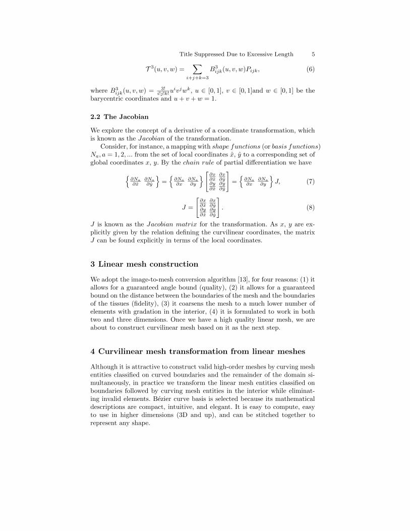
4.1 Constructing smooth Bezier paths from boundary meshentities

Fig. 1. Two Bezier paths with their control points (in green), made out of twoquadratic Bezier curves connected by the endpoints (in red). The yellow line seg-ments are tangents to the double sides of the red Bezier endpoint. Left: a smoothBezier path because the two green control points and the red endpoint lie in astraight line. Right: a Bezier path with a cusp where the curves connect, becausethe two green control points and the red endpoint do not lie in a straight line.

Fig. 2. An example of finding control points of a smooth cubic Bezier path. Forthe curve between P1 and P2, we need C2 and C3. On segment P0P2, find a pointQ1 such that|P0Q1|/|Q1P2|= |P0P1|/|P1P2|. Translate segment P0P2 so that pointQ1 lies on point P1, and scale the length of translated segment P0P2, then the newposition of point P2 is the position of control point C2. Similarly, the position ofcontrol point C3 can be found by translating segment P1P3 so that point Q2 lies onpoint P2.


A curve or surface can be described as having Gn continuity, n being themeasure of smoothness. Consider the segments on either side of a point on acurve:

G0: The curves touch at the join point.G1: The curves also share a common tangent direction at the join point.

We aim to find a smooth G1 curve passing through all the mesh boundarypoints given in order. A Bezier path is smooth provided that each endpointand its two surrounding control points lie in a straight line. In other words,the two tangents at each Bezier endpoint are parallel. Fig. 1 shows two Bezierpaths with their control points.

The basic idea is to calculate control points around each endpoint so thatthey lie in a straight line with the endpoint. However, curved segments wouldnot flow smoothly together when quadratic Bezier form (three control points)is used. Instead, we need to go one order higher to a cubic Bezier (four controlpoints) so we can build ”S” shaped segments.

The points we have in hand are only endpoints of boundary segments, sothe task becomes to find the other two control points to define the Beziercurve. We find these control points by translating the segments formed by thelines between the previous endpoint and the next endpoint such that thesesegments become the tangents of the curve at the endpoints. We scale thesesegments to control the curvature. An example is illustrated in Fig. 2.

4.2 Curving mesh entities in the interior

Fig. 3. Invalid elements.

It is usually not enough to curve only the boundary mesh edges becauseself-intersecting mesh edges may appear which lead to invalid elements. In such


cases, interior mesh elements should also be curved to eliminate the invalidity.Fig. 3 gives an example of such an occasion. Local mesh modifications suchas minimizing the deformation, edge or facet deletion, splitting, collapsing,swapping as well as shape manipulation have been used to correct an invalidregion [14, 8, 10, 12].

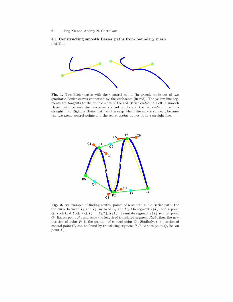
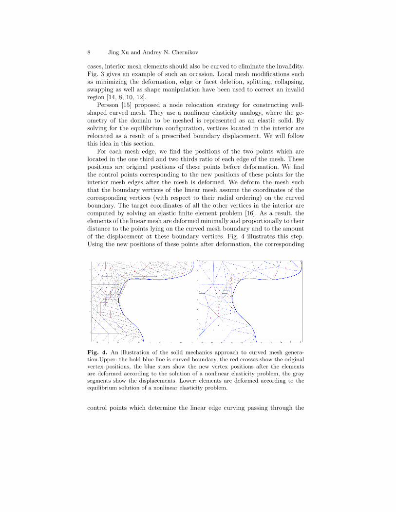
Persson [15] proposed a node relocation strategy for constructing well-shaped curved mesh. They use a nonlinear elasticity analogy, where the ge-ometry of the domain to be meshed is represented as an elastic solid. Bysolving for the equilibrium configuration, vertices located in the interior arerelocated as a result of a prescribed boundary displacement. We will followthis idea in this section.

For each mesh edge, we find the positions of the two points which arelocated in the one third and two thirds ratio of each edge of the mesh. Thesepositions are original positions of these points before deformation. We findthe control points corresponding to the new positions of these points for theinterior mesh edges after the mesh is deformed. We deform the mesh suchthat the boundary vertices of the linear mesh assume the coordinates of thecorresponding vertices (with respect to their radial ordering) on the curvedboundary. The target coordinates of all the other vertices in the interior arecomputed by solving an elastic finite element problem [16]. As a result, theelements of the linear mesh are deformed minimally and proportionally to theirdistance to the points lying on the curved mesh boundary and to the amountof the displacement at these boundary vertices. Fig. 4 illustrates this step.Using the new positions of these points after deformation, the corresponding

Fig. 4. An illustration of the solid mechanics approach to curved mesh genera-tion.Upper: the bold blue line is curved boundary, the red crosses show the originalvertex positions, the blue stars show the new vertex positions after the elementsare deformed according to the solution of a nonlinear elasticity problem, the graysegments show the displacements. Lower: elements are deformed according to theequilibrium solution of a nonlinear elasticity problem.

control points which determine the linear edge curving passing through the


points in the new positions can be easily calculated:

C1 = −5

6v0 +

1

3v1 + 3v3 −

3

2v4, (9)

C2 =1

3v0 −

5

6v1 −

3

2v3 + 3v4, (10)

where C1 and C2 are two middle control points of the four control points ofthe interior mesh edge, and v0, v1, v2 and v3 are points the curved edge willpass through.

Validity check is executed after this procedure. In most cases, it can han-dle this problem successfully. However, in the case that the curvature of theboundary edge is very large, the interior linear edge may not be curved enoughto avoid the intersection. Once our validity checking procedure reports thatthere is an intersected edge, local mesh modifications can be used to correctthe shape.

Because each curved edge has two control points in the middle, and eachcontrol point determines the curvature of the corresponding half of the edge,we first distinguish which part of the curved edge is intersected. For example,if the left half of the curved edge is intersected, that means the curvaturedetermined by the corresponding control point is not large enough. We enlargethe curvature by rotating the segment formed by the left endpoint and the leftcontrol point around the left endpoint by a small angle α. We do it repeatedlyuntil there is no intersection at all.

5 Element validity

A Curvilinear Mesh is valid provided that any two elements do not intersect(except the common vertices and edges). To verify a curved element, we canuse explicit intersection checks if the number of elements is small. A cheaperway is detecting the intersection at the element level by evaluating the sign ofthe determinant of the Jacobian matrix throughout the element. One approachis verifying the positiveness by sampling the Jacobian at discrete locations.A more efficient way is to calculate a lower bound for the determinant ofthe Jacobian. It is easy to be obtained when the Bezier form is used whenmapping a reference element due to its convex hull property [19]. In the casethat a positive bound is obtained, it guarantees that the element is valid; onthe contrary, when a non-positive bound occurs, the element could be invalid.In this case we need to obtain a tighter bound. This evaluation can be eitherused to check the validity or to guide the correction of invalid elements.

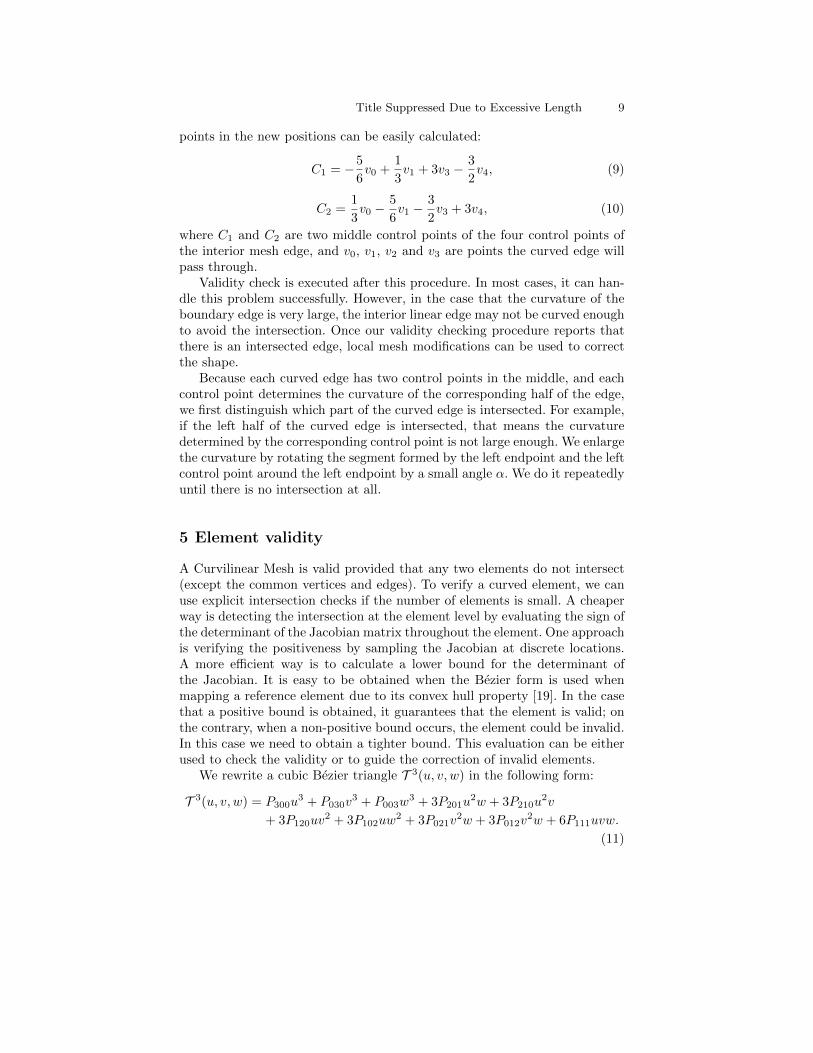
We rewrite a cubic Bezier triangle T 3(u, v, w) in the following form:

T 3(u, v, w) = P300u3 + P030v

3 + P003w3 + 3P201u

2w + 3P210u2v

+ 3P120uv2 + 3P102uw

2 + 3P021v2w + 3P012v

2w + 6P111uvw.

(11)


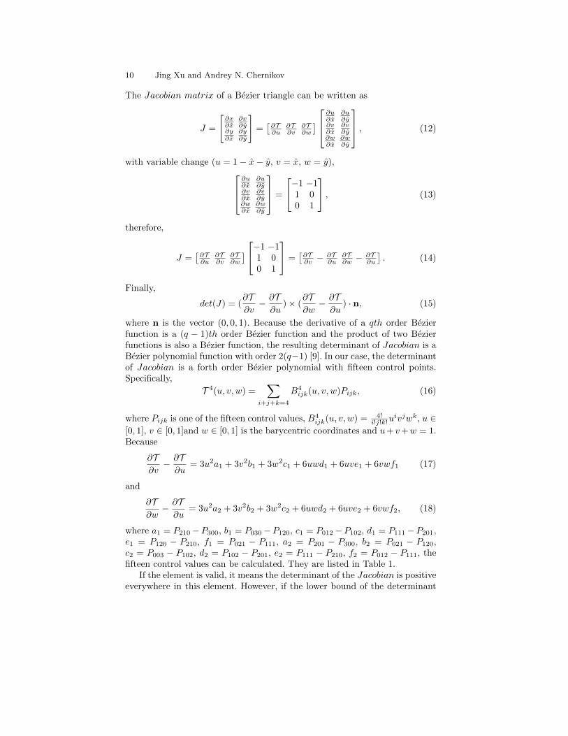
The Jacobian matrix of a Bezier triangle can be written as

J =

[∂x∂x

∂x∂y

∂y∂x

∂y∂y

]=[∂T∂u

∂T∂v

∂T∂w

] ∂u∂x

∂u∂y

∂v∂x

∂v∂y

∂w∂x

∂w∂y

, (12)

with variable change (u = 1− x− y, v = x, w = y),

(13)

∂u∂x

∂u∂y

∂v∂x

∂v∂y

∂w∂x

∂w∂y

=

−1 −11 00 1

,therefore,

J =[∂T∂u

∂T∂v

∂T∂w

] −1 −11 00 1

=[∂T∂v −

∂T∂u

∂T∂w −

∂T∂u

]. (14)

Finally,

det(J) = (∂T∂v− ∂T∂u

)× (∂T∂w− ∂T∂u

) · n, (15)

where n is the vector (0, 0, 1). Because the derivative of a qth order Bezierfunction is a (q − 1)th order Bezier function and the product of two Bezierfunctions is also a Bezier function, the resulting determinant of Jacobian is aBezier polynomial function with order 2(q−1) [9]. In our case, the determinantof Jacobian is a forth order Bezier polynomial with fifteen control points.Specifically,

T 4(u, v, w) =∑

i+j+k=4

B4ijk(u, v, w)Pijk, (16)

where Pijk is one of the fifteen control values, B4ijk(u, v, w) = 4!

i!j!k!uivjwk, u ∈

[0, 1], v ∈ [0, 1]and w ∈ [0, 1] is the barycentric coordinates and u+ v+w = 1.Because

∂T∂v− ∂T∂u

= 3u2a1 + 3v2b1 + 3w2c1 + 6uwd1 + 6uve1 + 6vwf1 (17)

and

∂T∂w− ∂T∂u

= 3u2a2 + 3v2b2 + 3w2c2 + 6uwd2 + 6uve2 + 6vwf2, (18)

where a1 = P210−P300, b1 = P030−P120, c1 = P012−P102, d1 = P111−P201,e1 = P120 − P210, f1 = P021 − P111, a2 = P201 − P300, b2 = P021 − P120,c2 = P003 − P102, d2 = P102 − P201, e2 = P111 − P210, f2 = P012 − P111, thefifteen control values can be calculated. They are listed in Table 1.

If the element is valid, it means the determinant of the Jacobian is positiveeverywhere in this element. However, if the lower bound of the determinant


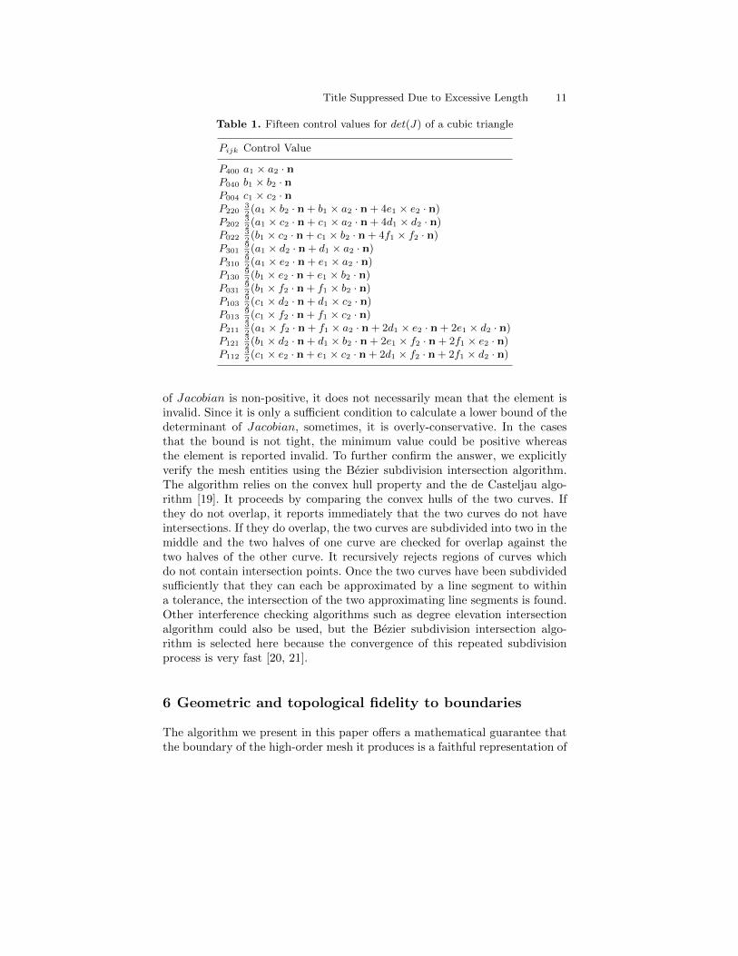
Table 1. Fifteen control values for det(J) of a cubic triangle

Pijk Control Value

P400 a1 × a2 · nP040 b1 × b2 · nP004 c1 × c2 · nP220

32(a1 × b2 · n + b1 × a2 · n + 4e1 × e2 · n)

P20232(a1 × c2 · n + c1 × a2 · n + 4d1 × d2 · n)

P02232(b1 × c2 · n + c1 × b2 · n + 4f1 × f2 · n)

P30192(a1 × d2 · n + d1 × a2 · n)

P31092(a1 × e2 · n + e1 × a2 · n)

P13092(b1 × e2 · n + e1 × b2 · n)

P03192(b1 × f2 · n + f1 × b2 · n)

P10392(c1 × d2 · n + d1 × c2 · n)

P01392(c1 × f2 · n + f1 × c2 · n)

P21132(a1 × f2 · n + f1 × a2 · n + 2d1 × e2 · n + 2e1 × d2 · n)

P12132(b1 × d2 · n + d1 × b2 · n + 2e1 × f2 · n + 2f1 × e2 · n)

P11232(c1 × e2 · n + e1 × c2 · n + 2d1 × f2 · n + 2f1 × d2 · n)

of Jacobian is non-positive, it does not necessarily mean that the element isinvalid. Since it is only a sufficient condition to calculate a lower bound of thedeterminant of Jacobian, sometimes, it is overly-conservative. In the casesthat the bound is not tight, the minimum value could be positive whereasthe element is reported invalid. To further confirm the answer, we explicitlyverify the mesh entities using the Bezier subdivision intersection algorithm.The algorithm relies on the convex hull property and the de Casteljau algo-rithm [19]. It proceeds by comparing the convex hulls of the two curves. Ifthey do not overlap, it reports immediately that the two curves do not haveintersections. If they do overlap, the two curves are subdivided into two in themiddle and the two halves of one curve are checked for overlap against thetwo halves of the other curve. It recursively rejects regions of curves whichdo not contain intersection points. Once the two curves have been subdividedsufficiently that they can each be approximated by a line segment to withina tolerance, the intersection of the two approximating line segments is found.Other interference checking algorithms such as degree elevation intersectionalgorithm could also be used, but the Bezier subdivision intersection algo-rithm is selected here because the convergence of this repeated subdivisionprocess is very fast [20, 21].

6 Geometric and topological fidelity to boundaries

The algorithm we present in this paper offers a mathematical guarantee thatthe boundary of the high-order mesh it produces is a faithful representation of


the geometric shape within a requested fidelity tolerance. We present proofsof the fact here.

The linear mesh constructed by the method in Sect. 3 provides a faithfulrepresentation of the underlying tissues. To measure the distance between theboundaries of the image tissues and the boundaries of the corresponding sub-mesh, we use the two-sided Hausdorff distance. This measure requires thatthe boundaries of the linear mesh are within the requested tolerance. Belowwe prove that the curved mesh boundary cannot deviate from the straightmesh boundary by more than a small multiple of the fidelity tolerance, andtherefore, for a given value of the fidelity tolerance, we can accommodate bothstraight and curved deviations. However, the supplied fidelity tolerance mustbe strictly positive.

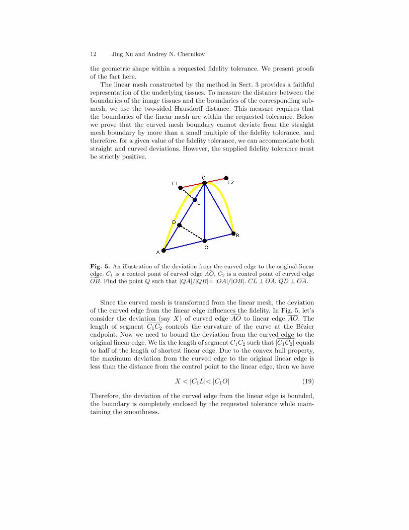
Fig. 5. An illustration of the deviation from the curved edge to the original linearedge. C1 is a control point of curved edge AO, C2 is a control point of curved edgeOB. Find the point Q such that |QA|/|QB|= |OA|/|OB|. CL ⊥ OA, QD ⊥ OA.

Since the curved mesh is transformed from the linear mesh, the deviationof the curved edge from the linear edge influences the fidelity. In Fig. 5, let’sconsider the deviation (say X) of curved edge AO to linear edge AO. Thelength of segment C1C2 controls the curvature of the curve at the Bezierendpoint. Now we need to bound the deviation from the curved edge to theoriginal linear edge. We fix the length of segment C1C2 such that |C1C2| equalsto half of the length of shortest linear edge. Due to the convex hull property,the maximum deviation from the curved edge to the original linear edge isless than the distance from the control point to the linear edge, then we have

X < |C1L|< |C1O| (19)

Therefore, the deviation of the curved edge from the linear edge is bounded,the boundary is completely enclosed by the requested tolerance while main-taining the smoothness.


7 Mesh examples

We apply our algorithm to a variety of examples in the following. For theseexamples, the input data is a two-dimensional image. The procedure describedin Sect. 4.2 was implemented in MATLAB. All the other steps were imple-mented in C++ for efficiency.

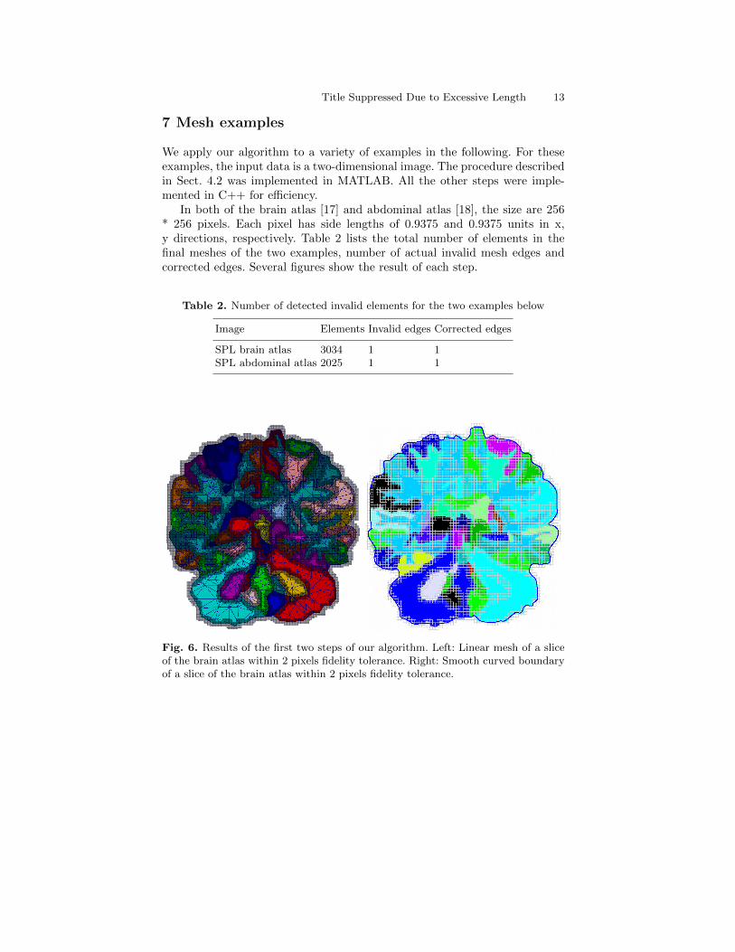
In both of the brain atlas [17] and abdominal atlas [18], the size are 256* 256 pixels. Each pixel has side lengths of 0.9375 and 0.9375 units in x,y directions, respectively. Table 2 lists the total number of elements in thefinal meshes of the two examples, number of actual invalid mesh edges andcorrected edges. Several figures show the result of each step.

Table 2. Number of detected invalid elements for the two examples below

Image Elements Invalid edges Corrected edges

SPL brain atlas 3034 1 1SPL abdominal atlas 2025 1 1

Fig. 6. Results of the first two steps of our algorithm. Left: Linear mesh of a sliceof the brain atlas within 2 pixels fidelity tolerance. Right: Smooth curved boundaryof a slice of the brain atlas within 2 pixels fidelity tolerance.


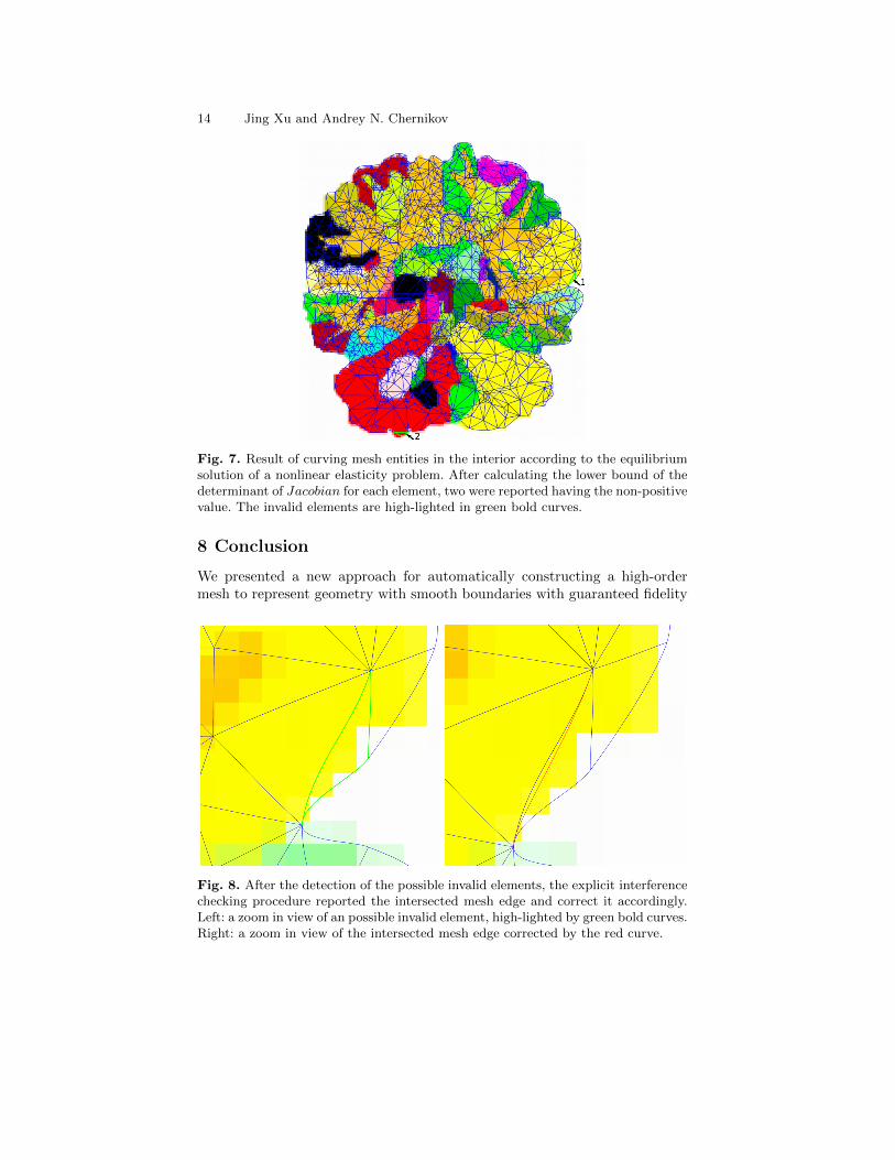
Fig. 7. Result of curving mesh entities in the interior according to the equilibriumsolution of a nonlinear elasticity problem. After calculating the lower bound of thedeterminant of Jacobian for each element, two were reported having the non-positivevalue. The invalid elements are high-lighted in green bold curves.

8 Conclusion

We presented a new approach for automatically constructing a high-ordermesh to represent geometry with smooth boundaries with guaranteed fidelity

Fig. 8. After the detection of the possible invalid elements, the explicit interferencechecking procedure reported the intersected mesh edge and correct it accordingly.Left: a zoom in view of an possible invalid element, high-lighted by green bold curves.Right: a zoom in view of the intersected mesh edge corrected by the red curve.


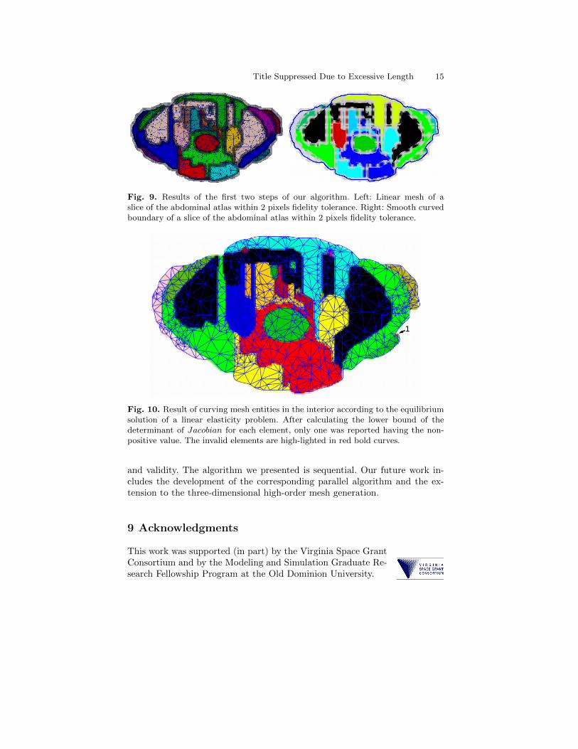
Fig. 9. Results of the first two steps of our algorithm. Left: Linear mesh of aslice of the abdominal atlas within 2 pixels fidelity tolerance. Right: Smooth curvedboundary of a slice of the abdominal atlas within 2 pixels fidelity tolerance.

Fig. 10. Result of curving mesh entities in the interior according to the equilibriumsolution of a linear elasticity problem. After calculating the lower bound of thedeterminant of Jacobian for each element, only one was reported having the non-positive value. The invalid elements are high-lighted in red bold curves.

and validity. The algorithm we presented is sequential. Our future work in-cludes the development of the corresponding parallel algorithm and the ex-tension to the three-dimensional high-order mesh generation.

9 Acknowledgments

This work was supported (in part) by the Virginia Space GrantConsortium and by the Modeling and Simulation Graduate Re-search Fellowship Program at the Old Dominion University.


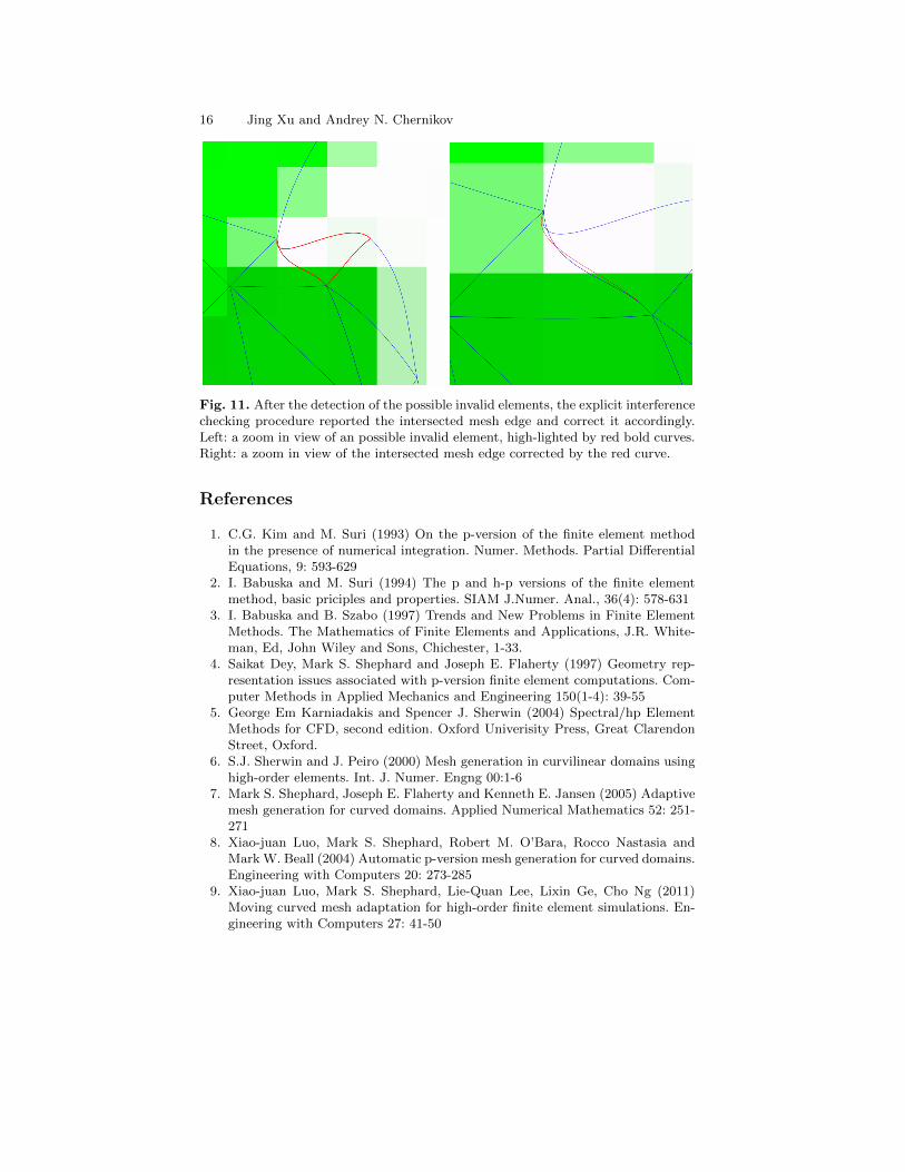
Fig. 11. After the detection of the possible invalid elements, the explicit interferencechecking procedure reported the intersected mesh edge and correct it accordingly.Left: a zoom in view of an possible invalid element, high-lighted by red bold curves.Right: a zoom in view of the intersected mesh edge corrected by the red curve.

References

1. C.G. Kim and M. Suri (1993) On the p-version of the finite element methodin the presence of numerical integration. Numer. Methods. Partial DifferentialEquations, 9: 593-629

2. I. Babuska and M. Suri (1994) The p and h-p versions of the finite elementmethod, basic priciples and properties. SIAM J.Numer. Anal., 36(4): 578-631

3. I. Babuska and B. Szabo (1997) Trends and New Problems in Finite ElementMethods. The Mathematics of Finite Elements and Applications, J.R. White-man, Ed, John Wiley and Sons, Chichester, 1-33.

4. Saikat Dey, Mark S. Shephard and Joseph E. Flaherty (1997) Geometry rep-resentation issues associated with p-version finite element computations. Com-puter Methods in Applied Mechanics and Engineering 150(1-4): 39-55

5. George Em Karniadakis and Spencer J. Sherwin (2004) Spectral/hp ElementMethods for CFD, second edition. Oxford Univerisity Press, Great ClarendonStreet, Oxford.

6. S.J. Sherwin and J. Peiro (2000) Mesh generation in curvilinear domains usinghigh-order elements. Int. J. Numer. Engng 00:1-6

7. Mark S. Shephard, Joseph E. Flaherty and Kenneth E. Jansen (2005) Adaptivemesh generation for curved domains. Applied Numerical Mathematics 52: 251-271

8. Xiao-juan Luo, Mark S. Shephard, Robert M. O’Bara, Rocco Nastasia andMark W. Beall (2004) Automatic p-version mesh generation for curved domains.Engineering with Computers 20: 273-285

9. Xiao-juan Luo, Mark S. Shephard, Lie-Quan Lee, Lixin Ge, Cho Ng (2011)Moving curved mesh adaptation for high-order finite element simulations. En-gineering with Computers 27: 41-50


10. P.L.George and H.Borouchaki (2012) Construction of tetrahedral meshes ofdegree two. Int. J. Numer. Mesh. Engng 90: 1156-1182

11. A. Johnen, J. F. Remacle and C. Geuzaine(2013) Geometrical validity of curvi-linear finite elements. Journal of Computational Physics 233: 359-372

12. Qiukai Lu, Mark S. Shephard, Saurabh Tendulkar and Mark W. Beall (2014)Parallel mesh adaptation for high-order finite element methods with curvedelement geometry. Engineering with Computers 30: 271-286

13. Andrey Chernikov and Nikos Chrisochoides (2011) Multitissue tetrahedralimage-to-mesh conversion with guaranteed quality and fidelity. SIAM Journalon Scientific Computing 33: 3491-3508

14. S. Dey, R.M.O’Bara and M.S. Shephard (2001) Towards curvilinear meshing in3D: the case of quadratic simplices. Computer-Aided Design 33: 199-209

15. Per-Olof Persson and Jaime Peraire (2009) Curved Mesh Generation and MeshRefinement using Lagrangian Solid Mechanics. In: Proceedings of the 47thAIAA Aerospace Sciences Meeting and Exhibit, Orlando (FL), USA, January5-9, 2009.

16. O. C. Zienkiewicz, R. L. Taylor, J. Z. Zhu (2005) The Finite Element Method:Its Basis and Fundamentals. 6th edition. Oxford: Butterworth-Heinemann.

17. I. Talos, M. Jakab, R. Kikinis, and M. Shenton (2008) SPL-PNL brain atlas.http://www.spl.harvard.edu/publications/item/view/1265.

18. I. Talos, M. Jakab, R. Kikinis, and M. Shenton (2008) SPL-PNL abdominalatlas. http://www.spl.harvard.edu/publications/item/view/1266.

19. Gerald Farin (1997) Curves and Surfaces for Computer-Aided Geometric De-sign. Academic Press.

20. E. Cohen and L. Schumaker (1985) Rates of convergence of control polygons.Computer Aided Geometric Design 2(1-3): 229-235

21. W. Dahmen (1986) Subdivision algorithm converge quadratically. J. of Com-putational and Applied Mathematics 16: 145-158

22. O. Sahni, X. J. Luo, K. E. Jansen, M. S. Shephard (2010) Curved boundarylayer meshing for adaptive viscous flow simulations. Finite Elements in Analysisand Design 46(1-2): 132-139

Automatic curvilinear mesh generation with smooth boundary … · 2014-08-13 · Automatic...

Documents

Transcript of Automatic curvilinear mesh generation with smooth boundary … · 2014-08-13 · Automatic...