Automatic Control Systems -Lecture Note...

1/25

Automatic Control Systems

Automatic Control Systems -Lecture Note 3-

Mathematical Foundation -1

2/25


Introduction

Mathematical model to analyze and control a complicated

dynamic system

Differential equation(DE)

Laplace transform can be used to solve linear differential

equation (LDE)

□ Introduction

3/25


Introduction

Mathematics

for

control system design

& analysis

Laplace Transform

Complex Variable Analysis

Differential Equation

Transfer Function Concept

Matrix Theory

4/25


Introduction

Approach to dynamic system problems

1. Identify target system and its components

2. Find its mathematical model along with assumptions needed

3. Earn and confirm its corresponding DE

4. Solve the DE for its output variable

5. Check the solution together with its assumptions

6. Review the model designed

5/25


DEs and Analogous Systems

Analogous Systems

- mathematical analogy with difference in physical properties

(Similar transfer function/DE)

- have the same form of solutions

- equivalent response to the same input

- a complex mechanical system can be simulated by using

the same type of analog/digital electric system model

6/25



Electrical vs Mechanical Systems

i) Analogy : force-voltage, mass-induction coil

7/25



o Serial mass-spring-damper (m-k-b) system dynamics

o Serial RLC circuit model

pkxdt

dxb

dt

xdm

2

2

2

2

1

1

diL Ri idt e

dt C

d q dqL R q e

dt dt C

8/25



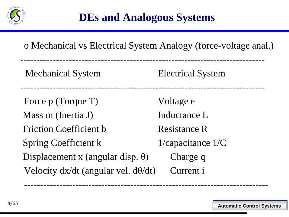
o Mechanical vs Electrical System Analogy (force-voltage anal.)

----------------------------------------------------------------------------

Mechanical System Electrical System

----------------------------------------------------------------------------

Force p (Torque T) Voltage e

Mass m (Inertia J) Inductance L

Friction Coefficient b Resistance R

Spring Coefficient k 1/capacitance 1/C

Displacement x (angular disp. θ) Charge q

Velocity dx/dt (angular vel. dθ/dt) Current i

----------------------------------------------------------------------------

9/25



ii) Analogy : force-current & mass-capacitor

10/25



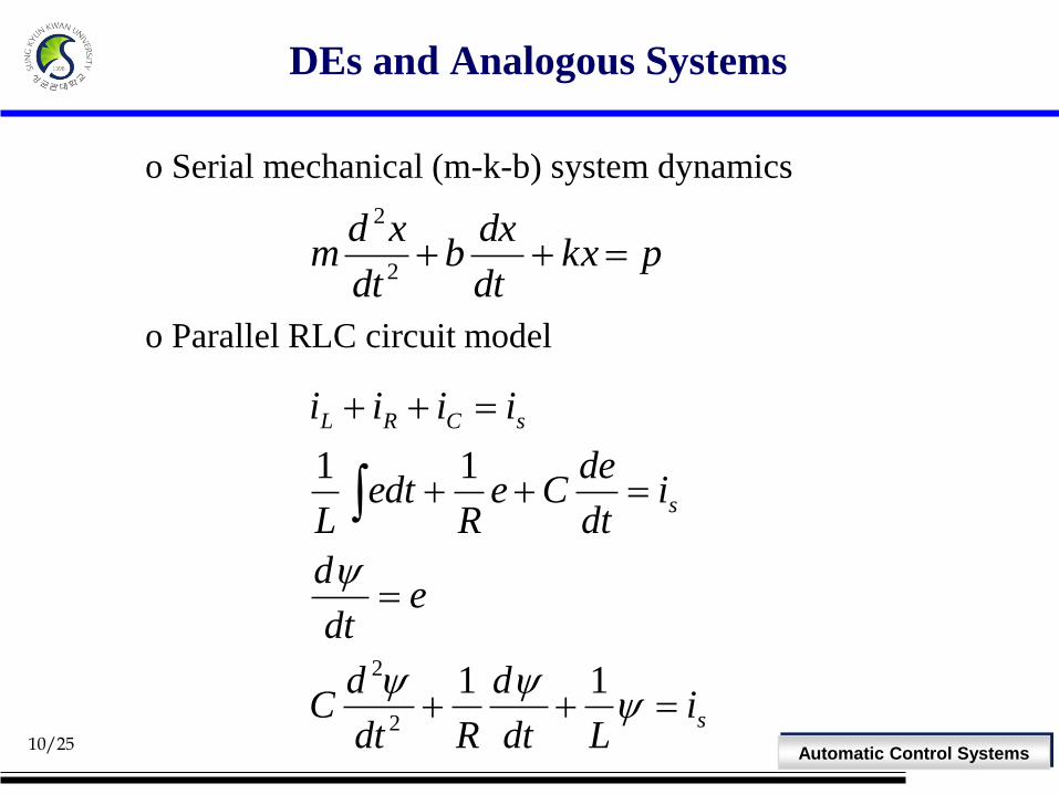
o Serial mechanical (m-k-b) system dynamics

o Parallel RLC circuit model

pkxdt

dxb

dt

xdm

2

2

s

s

sCRL

iLdt

d

Rdt

dC

edt

d

idt

deCe

Redt

L

iiii

11

11

2

2

11/25



o Mechanical vs Electrical System Analogy (force-current analogy)

----------------------------------------------------------------------------

Mechanical system Electrical system

----------------------------------------------------------------------------

force p (torque T) current i

mass m (inertia J) capacitance C

friction coefficient b 1/resistance 1/R

spring coefficient k 1/inductance 1/L

displacement x (angular disp. θ) magnetic flux Ψ

velocity dx/dt (angular vel. dθ/dt) voltage e

----------------------------------------------------------------------------

o The mathematical models of fluid, thermal, and mechanical systems are equivalent to electrical circuit model in that analogy exists in between their parameters.

12/25


Linear Approximation of Physical System

Nonlinear function z=f(x) can be linearized at around

the operating point P(x0,z0)

Taylor series is used for linearization

identify the corresponding Taylor series expansion

find the linearized form of function f(x)

13/25



Example : a reservoir water control system

/ Q K H R dH dQ 물의흐름이 이고 저항이 일때

Fig. (a) Liquid-level system: (b) Head versus flow rate curve.

In flow : Resistance :

14/25



1/ 2 1/ 21( ) ( )

2 2

2 2 2

/

2 ,

( ) /

KdQ d K H d KH K H dH dH

H

dH H H H h

dQ K Q qQ H

h HP R

q Q

Q Q H H R

점에서의기울기= Slope at P :

15/25


Laplace Transform

Foundation of Laplace transform was set by Laplace (1749-1827)

and its complete system was established by Heaviside (1850-

1925)

Can be used in solving LODE(linear ordinary differential

equation)

A complete solution of DE can be obtained for initial condition

and external input simultaneously

Can be used in obtaining the TF(transfer function) of LTI(linear

time invariant) system

A DE is converted into an AE(algebraic equation)

Differential eq algebraic eqL

16/25


Laplace Transform

Convolution integral algebraic multiplication

Definition

0( ) ( ) ( ) , stf t F s f t e dt s j

L

0( ) { ( )} ( ) , { }st

cF s f t f t e dt s R

L R

or

; unidirectional Laplace transform of piecewise continuous function f(t)

; s is complex variable, R{s} real part of s, Rc region of convergence

<Note> 1. Conversion of variables : 1/time = Hz 2. Laplace domain with complex s variable includes frequency domain of imaginary axis

17/25


Laplace Transform

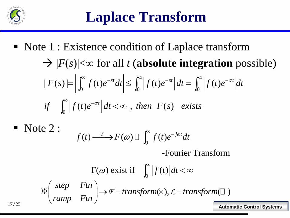
Note 1 : Existence condition of Laplace transform

|F(s)|<∞ for all t (absolute integration possible)

Note 2 :

0 0 0

0

| ( ) | ( ) ( ) ( )

( ) , ( )

st st t

t

F s f t e dt f t e dt f t e dt

if f t e dt then F s exists

0

0

( ) ( ) ( )

-Fourier Transform

F( ) exist if ( )

j tf t F f t e dt

f t dt

F

( ), ( )step Ftn

transform transformramp Ftn

※ F L

18/25


Laplace Transform

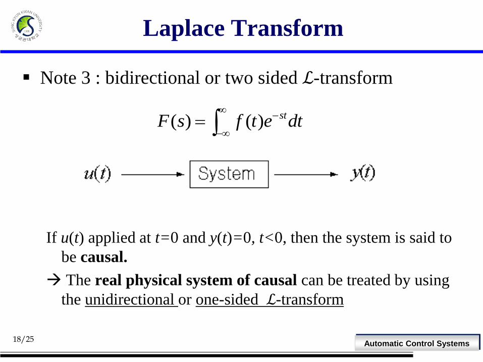
Note 3 : bidirectional or two sided ℒ-transform

If u(t) applied at t=0 and y(t)=0, t<0, then the system is said to

be causal.

The real physical system of causal can be treated by using

the unidirectional or one-sided ℒ-transform

( ) ( ) stF s f t e dt

19/25


Laplace Transform

Note 4 : another notation

0 0

-

( ) ( ) , ( ) ( )

( ) has an impulse at 0 ( ) ( )

otherwise, ( ) ( )

st stF s f t e dt F s f t e dt

f t t F s F s

F s F s

20/25


Laplace Transform

【Example】 unit-step function of constant signal

t

us(t)

1

0

0, 0( )

1, 0s

tu t

t

<Fig> unit-step function

21/25


Laplace Transform

Sol.)

O Existence condition?

0 0

0

0

( ) { ( )} ( ) 1

1 1[ ]

1, { } 0

st st

s s s

st

U s u t u t e dt e dt

e e es s

ss

L

R

( )

0 0

0

0

( ) ( )

( )

1 , 0

st j t

s s

t

s

t

u t e dt u t e dt

u t e dt

e dt for

22/25


Laplace Transform

【Example】 exponential function

Sol.)

0, 0( )

, 0at

tf t

ce t

0 0

( ) ( )

00

( ) { ( )} ( )

, { }

st at st

s a t s a t

F s f t f t e dt ce e dt

cce dt e

s a

cs a

s a

L

R

23/25


Laplace Transform

【Example】

【Example】

Sol.)

2

0, 0( )

, 0t t

tf t

e e t

1 1 (2 3)( )

1 2 ( 1)( 2)

sF s

s s s s

2 2

2 2

sin ,cos ?

1 1 1 1cos ( )

2 2

sin

j t j t

t t

st e e

s j s j s

ts

도 똑같은 방법으로 계산하면, 을 얻을 수 있음

L

L

can be transformed into

24/25


Laplace Transform

【Example】 delta function or impulse function

Sol.)

1, 0( ) ( )

0, . .

tf t t

o w

0( ) ( ) 1stF s t e dt

; identify the sifting property

25/25


Inverse Laplace Transform

; theoretic expression rather than practical

1

( ) ( )f t F s

L

L

1 1( ) [ ( )] ( )

2

c jst

c jf t F s F s e ds

j

L

□ Inverse Laplace Transform

Automatic Control Systems -Lecture Note...

Documents

Transcript of Automatic Control Systems -Lecture Note...