Automatic Complex Schema Matching across Web Query...

Automatic Complex Schema Matching across WebQuery Interfaces: A Correlation Mining Approach∗

Bin He, Kevin Chen-Chuan ChangComputer Science DepartmentUniversity of Illinois at [email protected], [email protected]

To enable information integration, schema matching is a critical step for discovering semanticcorrespondences of attributes across heterogeneous sources. While complex matchings are com-mon, because of their far more complex search space, most existing techniques focus on simple 1:1matchings. To tackle this challenge, this article takes a conceptually novel approach by viewingschema matching as correlation mining, for our task of matching Web query interfaces to inte-grate the myriad databases on the Internet. On this “deep Web,” query interfaces generally formcomplex matchings between attribute groups (e.g., {author} corresponds to {first name, last name}in the Books domain). We observe that the co-occurrences patterns across query interfaces oftenreveal such complex semantic relationships: grouping attributes (e.g., {first name, last name})tend to be co-present in query interfaces and thus positively correlated. In contrast, synonym at-tributes are negatively correlated because they rarely co-occur. This insight enables us to discovercomplex matchings by a correlation mining approach. In particular, we develop the DCM frame-work, which consists of data preprocessing, dual mining of positive and negative correlations, andfinally matching construction. We evaluate the DCM framework on manually extracted interfacesand the results show good accuracy for discovering complex matchings. Further, to automate theentire matching process, we incorporate automatic techniques for interface extraction. Execut-ing the DCM framework on automatically extracted interfaces, we find that the inevitable errorsin automatic interface extraction may significantly affect the matching result. To make the DCMframework robust against such “noisy” schemas, we integrate it with a novel “ensemble” approach,which creates an ensemble of DCM matchers, by randomizing the schema data into many trialsand aggregating their ranked results by taking majority voting. As a principled basis, we provideanalytic justification of the robustness of the ensemble approach. Empirically, our experimentsshow that the “ensemblization” indeed significantly boosts the matching accuracy, over automati-cally extracted and thus noisy schema data. By employing the DCM framework with the ensembleapproach, we thus complete an automatic process of matchings Web query interfaces.

Categories and Subject Descriptors: H.2.5 [Database Management]: Heterogeneous Databases; H.2.8 [Data-base Management]: Database Applications—Data Mining

General Terms: Algorithms, Measurement, Experimentation, Performance

Additional Key Words and Phrases: Data integration, schema matching, deep Web, correlationmining, ensemble, bagging predictors

1. INTRODUCTION

In recent years, we have witnessed the rapid growth of databases on the Web, or the so-called “deep Web.” A July 2000 survey [Bergman 2000] estimated that 96,000 “searchsites” and 550 billion content pages in this deep Web. Our recent study [Chang et al. 2004]in April 2004 estimated 450,000 online databases. With the virtually unlimited amount ofinformation sources, the deep Web is clearly an important frontier for data integration.

Schema matching is fundamental for supporting query mediation across deep Web sources.On the deep Web, numerous online databases provide dynamicquery-based data access

ACM Transactions on Database Systems, Vol. 31, No. 1, March 2006, Pages 1–45.

2 ·

(a) amazon.com (b) randomhouse.com (c) bn.com (d) 1bookstreet.com

Fig. 1. Example fragments of web query interfaces.

through theirquery interfaces, instead of static URL links. Each query interface acceptsqueries over itsquery schemas(e.g., author, title, subject, ... for amazon.com). Schemamatching (i.e., discovering semantic correspondences of attributes) across Web interfacesis essential for mediating queries across deep Web sources1.

In particular, matching Web interfaces in the same domain (e.g., Books, Airfares), thefocus of this article, is an important problem with broad applications. We often need tosearch over alternative sources in the same domain such as purchasing a book (or flightticket) across many online book (or airline) sources. Given a set of Web interfaces in thesame domain, this article addresses the problem of discovering matchings among thoseinterfaces. Section 2 will discuss some potential applications of our matching work andthe general abstraction of the matching problem. We note that our input, a set of Web pageswith interfaces in the same domain, can be either manually collected [Chang et al. 2003]or automatically generated [Ipeirotis et al. 2001].

On the “deep Web,” query schemas generally formcomplex matchingsbetween attributegroups. In contrast to simple 1:1 matching, complex matching matches a set ofm attributesto another set ofn attributes, which is thus also calledm:n matching. We observe that,in query interfaces, complex matchings do exist and are actually quite frequent. For in-stance, in the Books domain,author is a synonym of the grouping oflast name andfirstname, i.e., {author} = {first name, last name}; in the Airfares domain,{passengers}= {adults, seniors, children, infants}. Hence, discovering complex matchings is criticalto integrating the deep Web.

Although 1:1 matching has got great attention [Rahm and Bernstein 2001; Doan et al.2001; Madhavan et al. 2001; He and Chang 2003],m:n matching has not been extensivelystudied, mainly due to the much more complex search space of exploring all possiblecombinations of attributes (as Section 7 will discuss). To tackle this challenge, we investi-gate theco-occurrencepatterns of attributes across sources, to match schemasholistically.Unlike most schema matching work which matchestwo schemas in isolation, we matchall the schemas at the same time2. This holistic matching provides the co-occurrence in-formation of attributes across schemas and thus enables efficient mining-based solutions.For instance, we may observe thatlast name andfirst name often co-occur in schemas,while they together rarely co-occur withauthor, as Figure 1 illustrates. More generally,

1Note that our focus in this article is to match attributes across Web query interfaces. We believe this focus itselfis an interesting and challenging problem to study. Some subsequent and related problems, such as how to mapdata between sources after matching, how to decompose a user’s query onto specific sources and how to integratequery result pages from multiple sources, are also interesting topics to study but are beyond the scope of thiswork. Discussions about putting some of these tasks together as complete systems can be found at [Chang et al.2005] (i.e., the MetaQuerier system) and [Zhang et al. 2005] (i.e., the Form Assistant system), as Section 2 willbriefly discuss.2We note that, in the literature, the term “matching” was originally intended and also naturally suggests corre-spondences betweentwoschemas. In this paper, we take a broader view by considering matching, lacking a betterterm, as finding semantic correspondences among a set of schemas.

ACM Transactions on Database Systems, Vol. 31, No. 1, March 2006.

· 3

n-ary complex matchings{A} = {B} = {C, D, E}

{F, G} = {H, I}

****

********

*** *******

****

****

Data Preprocessing: type recognition and syntactic merging

Matching Discovery: dual correlation mining

Matching Construction: ranking and selection

Interface Extraction

��

Web pages with query interfaces

Fig. 2. From matching to mining: theDCM framework.

we observe thatgrouping attributes(i.e., attributes in one group of a matchinge.g., {lastname, first name}) tend to be co-present and thus positively correlated across sources. Incontrast,synonym attributes(i.e., attribute groups in a matching) are negatively correlatedbecause they rarely co-occur in schemas.

Note that by matching many schemas together, this holistic matching naturally discoversa more general type of complex matching – a matching may span across more than twoattribute groups. For instance, in Airfares domain, we may have the matching{adults,seniors, children, infants} = {passengers} = {number of tickets}, which is a 4:1:1matching. We name this type of matchingn-ary complex matching, which can be viewedas a composition of several binarym:n matchings.

These observations motivate us to develop a correlation mining abstraction of the schemamatching problem. Specifically, given extracted schemas from Web query interfaces, thisarticle develops a streamlined process, theDCM framework, for mining complex match-ings, consisting ofdata preprocessing, matching discoveryandmatching construction, asFigure 2 shows. Since the query schemas in Web interfaces are not readily minable inHTML format, before executing theDCM framework, we assume an interface extractorto extract the attribute information in the interfaces. For instance, the attribute abouttitlein Figure 1(c) can be extracted as〈name = “title of book”, domain = any〉, where “do-main = any” means any value is possible. (In this article, we will also address the impactof errors made by the automatic interface extractor on our matching algorithm.) Givenextracted raw schema data, we first preprocess schemas to make them ready for miningas the data preprocessing step (Section 3.3). Next, the matching discovery step, the coreof theDCM framework, explores adual correlation mining algorithm, which first minespotential attribute groups as positive correlations and then potential complex matchings asnegative correlations (Section 3.1). Finally, matching construction ranks and then selects


4 ·the most confident and consistent matchings from the mining result (Section 3.2). Mean-while, in the heart of correlation mining, we need to choose an appropriate correlationmeasure (Section 4).

Further, to complete an automatic matching process, which starts from raw HTML pagesas Figure 2 shows, we integrate theDCM framework with an automatic interface extrac-tor [Zhang et al. 2004]. Such “system integration” turns out to be non-trivial– As automaticinterface extraction cannot be perfect, it will introduce “noises” (i.e., erroneous extraction),which challenges the performance of the subsequent matching algorithm. As Section 5 willdiscuss, the errors in the interface extraction step may affect the correlations of matchingsand consequently the matching result. In particular, as we will show in the experiments(Section 6.2), the existence of noises may affect the matching accuracy up to 30%.

To make theDCM framework robust against noises, we integrate it with anensemblescheme, which aggregates a multitude of theDCM matchers to achieve robustness, byexploiting statistical sampling and majority voting. Specifically, we randomly sample asubset of schemas (as atrial ) to match, instead of using all the schemas. Intuitively, it islikely that such a trial still contains sufficient attribute information to match while remov-ing certain noisy schemas. Further, we conduct multiple independent trials. Since errors indifferent trials are independent, when noises are relatively few, it is likely that only a mi-nority of trials are affected. We thus take majority voting among the discovered matchingof all trials to achieve the robustness of holistic matching.

By employing theDCM framework with the ensemble approach, we thus complete anautomatic process of matching Web query interfaces. To evaluate the performance of ouralgorithms, we design two suites of experiments: First, to isolate and evaluate the effec-tiveness of theDCM framework, we test it on manually extracted TEL-8 dataset in theUIUC Web integration repository [Chang et al. 2003]. The matching result (Section 6.1)shows that theDCM framework achieves good accuracy with perfectly extracted schemasas input. Second, we test the ensembleDCM framework over automatically extracted in-terfaces in two domains, Books and Airfares, of the TEL-8 dataset. The result shows thatthe ensemble approach can significantly boost the matching accuracy under noisy schemainput, and thus maintain the desired robustness ofDCM (Section 6.2).

In summary, the contributions of this article are:• We build a conceptuallynovel connectionbetween the schema matching problem and

the correlation mining approach. On the one hand, we consider schema matching asa newapplicationof correlation mining; on the other hand, we propose correlationmining as a newapproachfor schema matching.

• We develop acorrelation measurethat is particularly suitable for negative correlation.In particular, we identify the problems of existing measures on evaluating negativecorrelation, which has special importance in schema matching, and further introduce anew correlation measure,H-measure.

• We employ anensemble schemeto connect theDCM framework with automatic inter-face extractor and thus fully automate the process of matching Web query interfaces. Inparticular, we identify the need for robust matching and integrate theDCM frameworkwith an ensemble approach by exploiting sampling and voting techniques.

The rest of the article is organized as follows: Section 2 discusses some potential ap-plications of our matching work and further abstracts the problem of matching Web queryinterfaces. Section 3 develops the baseDCM framework. Section 4 proposes a new correla-


· 5

tion measure. Section 5 motivates the need for robust matching and discusses the ensembleDCM framework. Section 6 reports our experiments. Section 7 reviews related work andSection 8 concludes the article.

2. CONTEXT AND ABSTRACTION

We observe that our matching scenario,i.e., discovering matchings across “alternative”sources in the same domain (e.g., Books, Airfares), is useful with broad applications. Inthis section, we first discuss two interesting applications,MetaQuerierandForm Assistant,in Section 2.1 and then abstract the schema matching problem we are tackling throughoutthis article in Section 2.2.

2.1 Context

MetaQuerier: We may build a MetaQuerier [Chang et al. 2005] to integrate dynamicallydiscovered and selected alternative sources according to user’s queries (http://metaquerier.-cs.uiuc.edu). As [Chang et al. 2005] describes, the goal of the MetaQuerier project is tobuild a middleware system to help users find and query large scale deep Web sources. Twocritical parts of the MetaQuerier system needs the help of the result of matching query in-terfaces. First, the MetaQuerier needs to build a unified interface for each domain, throughwhich users can issue queries. As also pointed out in [Chang et al. 2005], our work is thebasis for building the unified interfaces,e.g., by selecting the most representative attributeamong all the attributes that are synonyms of each other. Second, the matchings can beused for improving the quality of source selection according to user’s search keywords byexpanding the keywords,e.g., author, with semantically related words in the matchingresult,e.g., writer. Note that in both usage cases, it is not necessary that the matchings be100% accurate. Although the higher accuracy the result is, the better quality of service wecan provide, matching errors can be tolerated in the MetaQuerier system.

Form Assistant: As another scenario, instead of developing a complete MetaQuerier sys-tem, we may build a Form Assistant toolkit [Zhang et al. 2005] to help users translatequeries from one interface to other relevant interfaces. For instance, if a user fills the queryform in amazon.com, the Form Assistant cansuggesttranslated queries for another inter-ested source such asbn.com. To enable such query translation, the Form Assistant needsto first find matching attributes between two interfaces. The matching algorithm in [Zhanget al. 2005] employs adomain thesaurus(in addition to simple syntactic similarity-basedmatching) that specifies the correspondences of attributes in the domain. As mentionedin [Zhang et al. 2005], our matching work can be exploited as an automatic way to con-struct the domain-specific thesauruses. Note that in this Form Assistant scenario, matchingand translation errors can be tolerated, since the objective is to reduce users’ effort byproviding the “best-effort” query suggestion. Users can correct the errors, if any, beforesending the query.

2.2 Abstraction

These potential application scenarios, as the context of our work, indicate a new abstractionfor schema matching,i.e., discovering semantic correspondences among a set, instead of apair, of schemas. As Section 7 will elaborate, existing automatic schema matching worksmostly focus on matchings between two schemas (e.g., [Madhavan et al. 2001; Doan et al.2001]). Based on this fact, the latest survey [Rahm and Bernstein 2001] abstracts schema


6 ·

Holistic Schema

Matching

S2:writertitlecategoryformat

S3:nametitlekeywordbinding

S1:authortitlesubjectISBN

Input: a set of schemas

Output: all the matchings

author = writer = name

subject = category

format = binding

Fig. 3. The holistic schema matching abstraction.

matching as pairwise similarity mappings between two input sources. In contrast, in largescale integration scenarios such as the MetaQuerier and the Form Assistant systems, theschema matching task needs to match many schemas of a domain at the same time andfind all matchings at once. We name this new matching settingholistic schema match-ing. As Figure 3 shows, holistic schema matching takes a set of schemas as input andoutputs all the matchings among the input schemas. Such a holistic view enables us to ex-plore thecontextinformation beyond two schemas (e.g., similar attributes across multipleschemas; co-occurrence patterns among attributes), which is not available when schemasare matched only in pairs.

Next, we give an abstraction of the sub-tasks of the matching problem. In general,schema matching can be decomposed into two sequential steps:Matching discoveryandmatching construction. To begin with, matching discovery is to find a set of matchingcandidates that are likely to be correct matchings by exploiting some matching algorithms.This step is often the main focus of schema matching works. Further, matching construc-tion will select the most confident and consistent subset of candidates as the final matchingresult. A simple score-based ranking of matchings and constraint-based selection strategyis often used in this construction step. Separating our matching problem into the two stepshelps to “modularize” our framework, by defining a clean interface between these mod-ules, so that alternative matching discovery (i.e., not necessarily correlation mining-based)or construction techniques can also be incorporated. We will more formally abstract thesetwo steps below.

Matching Discovery

We view a query interface as a flat schema with a set ofattribute entities. An attributeentity can be identified by attributename, type and domain(i.e., instance values). Be-fore matching, the data preprocessing step (Section 3.3) finds syntactically similar entitiesamong schemas. Each attribute entity is assigned a uniqueattribute identifier, which wewill simply refer to as attribute below. While the matching is over the attribute entities,for our illustration, we use the attribute name of each entity as the attribute identifier. Forinstance, the schema in Figure 1(c) is thus a set of two attribute entities, written as{title,author}.

Formally, we abstract the matching discovery step as:Given the input as a set of schemasI = {Q1, ..., QN} in the same domain, where each schemaQi is a set of attributes, findall the matching candidatesR = {M1, ..., MV }. Each candidateMj is an n-ary com-plex matchingGj1 = Gj2 = ... = Gjw , where eachGjk

is an attribute group (i.e., agroup of attributes that are semantically equivalent to another attribute or another groupof attributes) andGjk

⊆ ⋃Nt=1 Qi. Semantically, eachMj represents the synonym rela-

tionship of attribute groupsGj1 ,...,Gjw and eachGjkrepresents the grouping relationship

of attributes inGjk.


· 7

Sharing the same abstraction of holistic schema matching, different realizations for thematching discovery step have been proposed. In this article, we present a dual correlationmining algorithm for finding matchings as a specific realization. Other approaches includestatistical model discovery based approaches [He and Chang 2003], and clustering-basedapproaches [He et al. 2003; Wu et al. 2004], as Section 7 will discuss.

Matching Construction

Given a set of discovered matching candidatesR = {M1, ..., MV }, the matching con-struction step proceeds with two sub-steps: matchingranking and selection. First, thematching ranking phase sorts all the candidates with some ranking criterionC. Let usdenote the ranked matchings asRC = {Mt1 , ..., MtV

}. In most schema matching worksfor finding pairwise semantic correspondences of two schemas (e.g., [Doan et al. 2001;Madhavan et al. 2001]), the matching ranking phase is quite straightforward by directlyusing the scores computed in the matching discovery step to rank candidates. However, inour scenario of findingn-ary complex matchings, as Section 3.2 will discuss, we find sucha simple ranking strategy may not work well and thus develop a different scoring strategyfrom the one used for finding matching candidates.

Then, the matching selection phase selects a subset of candidates fromRC as the fi-nal output of the matching process. Most schema matching works, including ours (Sec-tion 3.2), select candidates based on some consistency constraints,e.g., two matching can-didates that conflict by covering the same attribute cannot co-exist in the selection. Refer-ence [Melnik et al. 2002] develops a candidate selection strategy based on not only suchconstraints but also some selection metrics, inspired by bipartite-graph matching.

We have discussed the abstraction of the matching discovery and matching constructionsteps in our holistic schema matching problem. We will elaborate our realizations of thesetwo steps in theDCM framework, together with the data preprocessing step, in the nextsection.

3. FROM MATCHING TO MINING: THE BASE DCM FRAMEWORK

In this section, we will present technical details of theDCM framework, based on theabstraction Section 2 described. (Section 5 will motivate and discuss a further enhance-ment, deploying theDCM framework with an ensemble scheme.) In particular, we firstfocus on the core steps– matching discovery and matching construction– in Section 3.1and Section 3.2 respectively, and then discuss the data preprocessing step in Section 3.3.

3.1 Matching Discovery: Dual Correlation Mining

We first discuss our development for the core ofDCM, i.e., the matching discovery step,as Section 2 identified. We develop a dual correlation mining algorithm, which discoverscandidates of complex matchings,i.e., R = {M1, ..., MV }, as mining positive and thennegative correlations among attributes across schemas. In particular, the dual correlationmining algorithm consists ofgroup discoveryandmatching discovery. First,group discov-ery: We minepositively correlated attributesto form potential attribute groups. A potentialgroup may not be eventually useful for matching; only the ones having synonym relation-ship (i.e., negative correlation) with other groups can survive. For instance, if all sourcesuselast name, first name, and notauthor, then the potential group{last name, firstname} is not useful because there is no matching (toauthor) needed. Second,matchingdiscovery: Given the potential groups (including singleton ones), we minenegatively cor-


8 ·related attribute groupsto form potentialn-ary complex matchings. A potential matchingmay not be considered as correct due to the existence of conflicts among matchings.

After group discovery, we need to add the discovered groups into the input schemasIto mine negative correlations among groups. (A single attribute is viewed as a group withonly one attribute.) Specifically, an attribute group is added into a schema if that schemacontains any attribute in the group. For instance, if we discover thatlast name andfirstname have grouping relationship, we consider{last name, first name} as an attributegroup, denoted byGlf for simplicity, and add it to any schema containing eitherlast nameor first name, or both. The intuition is that although a schema may not contain the entiregroup, it still partially covers the concept that the group denotes and thus should be countedin matching discovery for that concept. Note that we do not remove singleton groups{lastname} and{first name} when addingGlf , becauseGlf is only a potential group andmay not survive in matching discovery.

While group discovery works on individual attributes and matching discovery on at-tribute groups, they can share the same mining process. We use the term –items– torepresent both attributes and groups in the following discussion of mining algorithm.

Correlation mining, at the heart, requires a measure to gauge correlation of a set ofnitems; our observation indicates pairwise correlations among thesen items. Specifically,for n groups forming synonyms, any two groups should be negatively correlated, since theyboth are synonyms by themselves (e.g., in the matching{destination} = {to} = {arrivalcity}, negative correlations exist between any two groups). We have similar observationon the attributes with grouping relationships. Motivated by such observations, we designthe measure as:

Cmin({A1, ..., An},m) = min m(Ai, Aj), ∀i 6= j, (1)

wherem is some correlation measure for two items. That is, we defineCmin as the minimalvalue of the pairwise evaluation, thus requiring all pairs to meet this minimal “strength.”In principle, any correlation measure for two items is applicable asm (e.g., the measuressurveyed in [Tan et al. 2002]); However, since the semantic correctness of the miningresult is of special importance for our schema matching task, we develop a new measure,H-measure, which can better satisfy the quality requirements of measures (Section 4).

Cmin has several advantages: First, it satisfies the “apriori” feature and thus enablesthe design of an efficient algorithm. In correlation mining, the measure for qualificationpurpose should have a desirable “apriori” property (i.e., downward closure), to develop anefficient algorithm. (In contrast, a measure for ranking purpose should not have this apriorifeature, as Section 3.2 will discuss.)Cmin satisfies the apriori feature since given any itemsetA and its subsetA∗, we haveCmin(A, m) ≤ Cmin(A∗, m) because the minimum of alarger set (e.g., min({1,3,5})) cannot be higher than its subset (e.g., min({3,5})). Second,Cmin can incorporate any measurem for two items and thus can accommodate differenttasks (e.g., mining positive and negative correlations) and be customized to achieve goodmining quality.

With Cmin, we can directly define positively correlated attributes in group discoveryand negatively correlated attribute groups in matching discovery. A set of attributes{A1,..., An} is positively correlated attributes, if Cmin({A1, ...,An}, mp) ≥ Tp, wheremp isa measure for positive correlation andTp is a given threshold. Similarly, a set of attributegroups{G1, ...,Gm} is negatively correlated attribute groups, if Cmin({G1, ...,Gm}, mn)


· 9

Algorithm: APRIORICORRM INING:Input: Input SchemasI = {Q1, ..., QN}, Measurem, ThresholdTOutput: Correlated itemsbegin:1 X ← ∅2 /* First, find all correlated two items */3 /* V: the vocabulary of all items */4 V ← ∪N

t=1Qi, Qi ∈ I5 for all Ap, Aq ∈ V, p 6= q6 if m(Ap, Aq) ≥ T then X ← X ∪ {{Ap, Aq}}7 /* Then, build correlatedl + 1 items from correlatedl items */8 /* Xl: correlatedl items */9 l ← 210 Xl ← X11 while Xl 6= ∅12 Xl+1 ← ∅13 for each item groupY ∈ Xl

14 for each itemA ∈ V − Y15 /* Z: a candidate of correlatedl + 1 items */16 Z ← Y ∪ {A}17 /* Verify whetherZ is in fact a correlatedl + 1 items */18 Zl ← all subsets ofZ with sizel19 if Zl ⊂ Xl then Xl+1 ← Xl+1 ∪ Z20 X ← X ∪Xl+1

21 Xl ← Xl+1

21 l ← l + 122 return Xend

Fig. 4. Apriori algorithm for mining correlated items.

≥ Tn, wheremn is a measure for negative correlation andTn is another given threshold.As we will discuss in Section 4, although in principle any correlation measure can be usedasmp andmn, e.g., Lift andJaccard, to make matching result more accurate, we need todevelop a new correlation measure, which satisfies some crucial characteristics.

Leveraging the apriori feature ofCmin, we develop AlgorithmAPRIORICORRM INING

(Figure 4) for discovering correlated items, in the spirit of the classic Apriori algorithm forassociation mining [Agrawal et al. 1993]. Specifically, as the apriori feature indicates, if aset ofl+1 itemsA = {A1, ...,Al+1} satisfiesCmin(A, m)≥ T , then any subset ofA withsize more than one item, denoted asA∗, also satisfiesCmin(A∗, m) ≥ T . It can be shownthe the reverse argument is also true. Further, it can be shown that as long as any subsetof A with sizel, also denoted asA∗, satisfiesCmin(A∗, m) ≥ T , we haveCmin(A, m) ≥T [Agrawal et al. 1993].

Therefore, we can find all the correlated items with sizel+1 based on the ones with sizel. As Figure 4 shows, to start, we first find all correlated two items (Lines 4-6). Next, werepeatedly construct correlatedl+1 itemsXl+1 from correlatedl itemsXl(Lines 9-22). Inparticular, for each correlatedl itemsY in Xl, we expandY to be a candidate of correlatedl +1 items, denoted asZ, by adding a new attributeA (Line 16). We then test whether any


10 ·Algorithm: DUAL CORRELATIONM INING:Input: Input SchemasI = {Q1, ..., QN}, Measuresmp,mn, ThresholdsTp, Tn

Output: Potentialn-ary complex matchingsbegin:1 /* group discovery */2 G ← APRIORICORRM INING(I, mp, Tp)3 /* adding groups intoI */4 for eachQi ∈ I5 for eachGk ∈ G6 if Qi ∩Gk 6= ∅ then Qi ← Qi ∪ {Gk}7 /* matching discovery */8 R ← APRIORICORRM INING(I,mn, Tn)9 return Rend

Fig. 5. Algorithm for mining complex matchings.

subset ofZ with sizel is found inXl. If so, Z is a correlatedl + 1 items and added intoXl+1 (Lines 18-19).

Algorithm DUAL CORRELATIONM INING shows the pseudo code of the complex match-ing discovery (Figure 5). Line 2 (group discovery) callsAPRIORICORRM INING to minepositively correlated attributes. Lines 3-6 add the discovered groups intoI. Line 8 (match-ing discovery) callsAPRIORICORRM INING to mine negatively correlated attribute groups.Similar to [Agrawal et al. 1993], the time complexity ofDUAL CORRELATIONM INING isexponential with respect to the number of attributes. But in practice, the execution is quitefast since correlations exist among semantically related attributes, which is far less thanarbitrary combination of all attributes.

3.2 Matching Construction: Majority-based Ranking and Constraint-based Se-lection

After the matching discovery step, we need to develop ranking and selection strategiesfor the matching construction step, as Section 2 described. We notice that the matchingdiscovery step can discover true semantic matchings and, as expected, also false ones dueto the existence of coincidental correlations. For instance, in the Books domain, the resultof correlation mining may have both{author} = {first name, last name}, denoted byM1 and{subject} = {first name, last name}, denoted byM2. We can seeM1 is correct,while M2 is not. The reason for having the false matchingM2 is that in the schema data,it happens thatsubject does not often co-occur withfirst name andlast name.

The existence of false matchings may cause matching conflicts. For instance,M1 andM2 conflict in that if one of them is correct, the other one should not. Otherwise, we get awrong matching{author} = {subject} by the transitivity of synonym relationship. Sinceour mining algorithm does not discover{author} = {subject}, M1 andM2 cannot be bothcorrect.

Leveraging such conflicts, we select the most confident and consistent matchings to re-move the false ones. Intuitively, between conflicting matchings, we want to select the morenegatively correlated one because it indicates higher confidence to be real synonyms. Forexample, our experiment shows that, asM2 is coincidental, it is indeed thatmn(M1) >mn(M2), and thus we selectM1 and removeM2. Note that, with larger data size, seman-


· 11

tically correct matching is more possible to be the winner. The reason is that, with largersize of sampling, the correct matchings are still negatively correlated while the false oneswill remain coincidental and not as strong.

Therefore, as Section 2 abstracted, the matching construction step consists of two phases:1) Matching ranking: We need to develop a strategy to reasonably rank to discoveredmatchings in the dual correlation mining. 2)Matching selection: We need to develop aselection algorithm to select the ranked matchings. We will elaborate these two phases inthis subsection respectively.

Matching Ranking

To begin with, we need to develop a strategy forranking the discovered matchingsR.That is, for anyn-ary complex matchingMj in R: Gj1 = Gj2 = ... = Gjw , we have ascoring functions(Mj ,mn) to evaluateMj under measuremn and output a ranked list ofmatchingsRC .

While Section 3.1 discussed a measure for “qualifying” candidates, we now need todevelop another “ranking” measure as the scoring function. Since ranking and qualificationare different problems and thus require different properties, we cannot apply the measureCmin (Equation 1) for ranking. Specifically, the goal of qualification is to ensure thecorrelations passing some threshold. It is desirable for the measure to support downwardclosure to enable an “apriori” algorithm. In contrast, the goal of ranking is to compare thestrength of correlations. The downward closure enforces, by definition, that a larger itemset is always less correlated than its subsets, which is inappropriate for ranking correlationsof different sizes. Hence, we develop another measureCmax, the maximalmn valueamong pairs of groups in a matching, as the scoring functions. Formally,

Cmax(Mj ,mn) = max mn(Gjr , Gjt), ∀Gjr , Gjt , jr 6= jt. (2)

It is possible to get ties if only considering theCmax value; we thus develop a naturalstrategy for tie breaking. We take a “top-k” approach so thats in fact is a set of sortedscores. Specifically, given matchingsMj andMk, if Cmax(Mj , mn) = Cmax(Mk, mn),we further compare their second highestmn values to break the tie. If the second highestvalues are also equal, we compare the third highest ones and so on, until breaking the tie.

If two matchings are still tie after the “top-k” comparison, we choose the one with richersemantic information. We consider matchingMj semantically subsumesmatchingMk,denoted byMj º Mk, if all the semantic relationships inMk are covered inMj . Forinstance,{arrival city} = {destination} = {to} º {arrival city} = {destination} be-cause the synonym relationship in the second matching is subsumed in the first one. Also,{author} = {first name, last name} º {author} = {first name} because the synonymrelationship in the second matching is part of the first.

Combining the scoring function and the semantic subsumption, we rank matchings withfollowing rules: 1) If s(Mj ,mn) > s(Mk,mn), Mj is ranked higher thanMk. 2) Ifs(Mj ,mn) = s(Mk,mn) andMj º Mk, Mj is ranked higher thanMk. 3) Otherwise, werankMj andMk arbitrarily.

Matching Selection

Given matchingsRC = {M1, ...,MV } ranked according to the above ranking strategy,we next develop a greedy matching selection algorithm as follows:

1. Among the remaining matchings inRC , choose the highest ranked matchingMt.ACM Transactions on Database Systems, Vol. 31, No. 1, March 2006.

12 ·2. Remove matchings conflicting withMt in RC .3. If RC is empty, stop; otherwise, go to step 1.

Specifically, we select matchings with multiple iterations. In each iteration, we greed-ily choose the matching with the highest rank and remove its conflicting matchings. Theprocess stops until no matching candidate is left. Example 1 illustrates this greedy se-lection algorithm with a concrete example. The time complexity of the entire matchingconstruction process isO(V 2), whereV is the number of matchings inRC .

Example 1: Assume runningDUAL CORRELATIONM INING in the Books domain findsmatchingsRC as (matchings are followed by theirCmax scores):

M1: {author} = {last name, first name}, 0.95M2: {author} = {last name}, 0.95M3: {subject} = {category}, 0.92M4: {author} = {first name}, 0.90M5: {subject} = {last name, first name} , 0.88M6: {subject} = {last name}, 0.88 andM7: {subject} = {first name}, 0.86.According to our ranking strategy, we will rank these matchings asM1 > M2 > M3 >

M4 > M5 > M6 > M7 in descending order. In particular, althoughs(M1, mn) =s(M2,mn), M1 is ranked higher sinceM1 º M2. Next, we select matchings with thegreedy strategy: In the first iteration,M1 is selected since it is ranked the highest. Thenwe need to remove matchings that conflict withM1. For instance,M2 conflicts withM1

onauthor and thus should be removed fromRC . Similarly,M4 andM5 are also removed.The remaining matchings areM3, M6 andM7. In the second iteration,M3 is ranked thehighest and thus selected.M6 andM7 are removed because they conflict withM3. NowRC is empty and the algorithm stops. The final output is thusM1 andM3.

3.3 Data Preprocessing

As input of theDCM framework, we assume an interface extractor (Figure 2) has extractedattribute information from Web interfaces in HTML formats. For instance, the attributeabout title in Figure 1(c) and Figure 1(d) can be extracted as〈name = “title of book”,domain = any〉 and〈name = “search for a specific title”, domain = any〉 respectively, where“domain = any” means any value is possible. Section 5 will discuss the incorporation ofan automatic interface extractor [Zhang et al. 2004].

As we can see from the above examples, the extracted raw schemas contain many syn-tactic variations around the “core” concept (e.g., title) and thus are not readily minable. Wethus perform a data preprocessing step to make schemas ready for mining. The data pre-processing step consists ofattribute normalization, type recognitionandsyntactic merging.To begin with, given extracted schema data, we perform some standard normalization onthe extracted names and domain values. We first stem attribute names and domain valuesusing the standard Porter stemming algorithm [Porter ]. Next, we normalize irregular nounsand verbs (e.g., “children” to “child,” “colour” to “color”). Last, we remove common stopwords by a manually built stop word list, which contains words common in English, inWeb search (e.g., “search”, “page”), and in the respective domain of interest (e.g., “book”,“movie”).

We then perform type recognition to identify attribute types. As Section 3.3.1 discusses,type information helps to identify homonyms (i.e., two attributes may have the same name


· 13

any

string integer

float

month day time

date

datetime

Fig. 6. The compatibility of types.

but different types) and constrain syntactic merging and correlation-based matching (i.e.,only attributes with compatible types can be merged or matched). Since the type infor-mation is not declared in Web interfaces, we develop atype recognizerto recognize typesfrom domain values.

Finally, we merge attribute entities by measuring the syntactic similarity of attributenames and domain values (e.g., we merge “title of book” to “title” by name similarity). Itis a common data cleaning technique to merge syntactically similar entities by exploringlinguistic similarities. Section 3.3.2 discusses our merging strategy.

3.3.1 Type Recognition.While attribute names can distinguish different attribute enti-ties, the names alone sometimes lead to the problem of homonyms (i.e., the same namewith different meanings) – we address this problem by distinguishing entities by bothnames and types. For instance, the attribute namedeparting in the Airfares domain mayhave two meanings: a datetime type as departing date, or a string type as departing city.With type recognition, we can recognize that there are two different types ofdeparting:departing (datetime) anddeparting (string), which indicate two attribute entities.

In general, type information, as a constraint, can help the subsequent steps of syntacticmerging and correlation-based matching. In particular, if the types of two attributes arenot compatible, we consider they denote different attribute entities and thus neither mergethem nor match them.

Since type information is not explicitly declared in Web interfaces, we develop atyperecognizerto recognize types from domain values of attribute entities. For example, a listof integer values denotes an integer type. In the current implementation, type recognitionsupports the following types: any, string, integer, float, month, day, date, time and date-time. (An attribute with only an input box is given an any type since the input box canaccept data with different types such as string or integer.) Two types arecompatibleifone can subsume another (i.e., the is-a relationship). For instance, date and datetime arecompatible since date subsumes datetime. Figure 6 lists the compatibility of all the typesin our implementation.

3.3.2 Syntactic Merging.We clean the schemas by merging syntactically similar at-tribute entities, a common data cleaning technique to identify unique entities [Chaudhuriet al. 2003]. Specifically, we developname-based merginganddomain-based mergingbymeasuring the syntactic similarity of attribute names and domains respectively. Syntacticmerging increases the observations of attribute entities, which can improve the effect ofcorrelation evaluation.

Name-based Merging: We merge two attribute entities if they are similar in names.We observe that the majority of deep Web sources are consistent on some concise “core”attribute names (e.g., “title”) and others are variation of the core ones (e.g., “title of book”).Therefore, we consider attributeAp to bename-similarto attributeAq if Ap’s name⊇Aq ’s


14 ·Ap ¬Ap

Aq f11 f10 f1+

¬Aq f01 f00 f0+

f+1 f+0 f++

Fig. 7. Contingency table for test of correlation.

name (i.e., Ap is a variation ofAq) andAq is more frequently used thanAp (i.e., Aq is themajority). This frequency-based strategy helps avoid false positives. For instance, in theBooks domain,last name is not merged toname becauselast name is more popularthanname and thus we consider them as different entities.

Domain-based Merging: We then merge two attribute entities if they are similar indomain values. For query interfaces, we consider the domain of an attribute as the valuesthat the attribute can select from. Such values are often presented in a selection list or aset of radio buttons in a Web form. In particular, we only consider attributes with stringtypes, since it is unclear how useful it is to measure the domain similarity of other types.For instance, in the Airfares domain, the integer values ofpassengers andconnectionsare quite similar, although they denote different meanings.

We view domain values as a bag of words (i.e., counting the word frequencies). We namesuch a bagaggregate values, denoted asVA for attributeA. Given a wordw, we denoteVA(w) as the frequency ofw in VA. The domain similarity of attributesAp andAq is thusthe similarity ofVAp andVAq . In principle, any reasonable similarity function is applicable

here. In particular, we choosesim(Ap, Aq) = ∀w in both VAp and VAq ,VAp (w)+VAq (w)

∀w in either VAp or VAq ,VAp (w)+VAq (w) .

Example 2: Assume there are 3 schemas,S1 to S3, in the Airfares domain.S1 containsattribute entity〈name = “trip type”, type = “string”, domain ={“round trip”, “one way”}〉,S2 contains〈name = “trip type”, type = “string”, domain ={“round trip”, “one way”,“multi-city” }〉 andS3 contains〈name = “ticket type”, type = “string”, domain ={“roundtrip”, “one way”}〉.

The attribute entitytrip type (string) occurs inS1 andS2 and thus its aggregate valuesVtrip type = {round: 2, trip: 2, one: 2, way: 2, multi: 1, city: 1}, where each word is followedby frequency. In particular,Vtrip type(round) = 2 since the word “round” uses in bothS1

andS2. Similarly, Vticket type = {round: 1, trip: 1, one: 1, way: 1}. Then, according to oursimilarity function, we havesim(trip type, ticket type) = 3+3+3+3

3+3+3+3+1+1 =0.86.

4. CORRELATION MEASURE

Since we are pursuing a mining approach, we need to choose an appropriate correlationmeasure. In particular, to complete our development of theDCM framework, we nowdiscuss the positive measuremp and the negative measuremn, which are used as thecomponents ofCmin (Equation 1) for positive and negative correlation mining respectively(Section 3.1).

As discussed in [Tan et al. 2002], a correlation measure by definition is a testing on thecontingency table. Specifically, given a set of schemas and two specified attributesAp andAq, there are four possible combinations ofAp andAq in one schemaSi: Ap, Aq are co-present inSi, only Ap presents inSi, only Aq presents inSi, andAp, Aq are co-absent inSi. Thecontingency table[Brunk 1965] ofAp andAq contains the number of occurrencesof each situation, as Figure 7 shows. In particular,f11 corresponds to the number of co-presence ofAp andAq; f10, f01 andf00 are denoted similarly.f+1 is the sum off11 and


· 15

0

10

20

30

40

50

60

10 20 30 40 50N

umbe

r of

Obs

erva

tions

Attributes in Books DomainFig. 8. Attribute frequencies in the Books domain.

f01; f+0, f0+ andf1+ are denoted similarly.f++ is the sum off11, f10, f01 andf00.The design of a correlation measure is often empirical. To our knowledge, there is no

good correlation measure universally agreed upon [Goodman and Kruskal 1979; Tan et al.2002]. For our matching task, in principleanymeasure can be applied. However, since thesemantic correctness of the mining result is of special importance for the schema match-ing task, we care more the ability of the measures on differentiating various correlationsituations, especially the subtlety of negative correlations, which has not been extensivelystudied before. In Section 4.1, we develop a new correlation measure,H-measure, whichis better than existing measures in satisfying our requirements. In Section 4.2, we fur-ther show thatH-measure satisfies a nice sampling invariance property, which makes thesetting of parameter threshold independent of the data size.

4.1 H-Measure

We first identify the quality requirements of measures, which are imperative for schemamatching, based on the characteristics of Web query interfaces. Specifically, we observethat, in Web interfaces, attribute frequencies are extremely non-uniform, similar to the useof English words, showing some Zipf-like distribution. For instance, Figure 8 shows theattribute frequencies in the Books domain: First, the non-frequent attributes results in thesparseness of the schema data (e.g., there are over 50 attributes in the Books domain, buteach schema only has 5 in average). Second, many attributes are rarely used, occurringonly once in the schemas. Third, there exist some highly frequent attributes, occurring inalmost every schema.

These three observations indicate that, as the quality requirements, the chosen measuresshould be robust against the following problems:sparseness problemfor both positiveand negative correlations,rare attribute problemfor negative correlations, andfrequentattribute problemfor positive correlations. In this section, we discuss each of them indetails.

The Sparseness Problem

In schema matching, it is more interesting to measure whether attributes are often co-present (i.e., f11) or cross-present (i.e., f10 andf01) than whether they are co-absent (i.e.,f00). Many correlation measures, such asχ2 andLift, include the count of co-absencein their formulas. This may not be good for our matching task, because the sparsenessof schema data may “exaggerate” the effect of co-absence. This problem has also beennoticed by recent correlation mining work such as [Tan et al. 2002; Omiecinski 2003; Lee


16 ·Ap ¬Ap

Aq 5 5 10¬Aq 5 85 90

10 90 100

Ap ¬Ap

Aq 1 49 50¬Aq 1 1 2

2 50 52

Ap ¬Ap

Aq 81 9 90¬Aq 9 1 10

90 10 100(a1)Example of sparseness problem(b1) Example of rare attribute problem (c1)Example of frequent attribute problem

with measureLift: with measureJaccard: with measureJaccard:Less positive correlation Ap as rare attribute Ap andAq are independentbut a higherLift = 17. andJaccard= 0.02. but a higherJaccard= 0.82.

Ap ¬Ap

Aq 55 20 75¬Aq 20 5 25

75 25 100

Ap ¬Ap

Aq 1 25 26¬Aq 25 1 26

26 26 52

Ap ¬Ap

Aq 8 1 9¬Aq 1 90 91

9 91 100(a2)Example of sparseness problem(b2) Example of rare attribute problem (c2)Example of frequent attribute problem

with measureLift: with measureJaccard: with measureJaccard:More positive correlation no rare attribute Ap andAq are positively correlatedbut a lowerLift = 0.69. andJaccard= 0.02. but a lowerJaccard= 0.8.

Fig. 9. Examples of the three problems.

et al. 2003]. In [Tan et al. 2002], the authors use thenull invarianceproperty to evaluatewhether a measure is sensitive to co-absence. The measures for our matching task shouldsatisfy this null invariance property.

Example 3: Figure 9(a) illustrates the sparseness problem with an example. In this exam-ple, we choose a common measure: theLift (i.e., Lift = f00f11

f10f01). (Other measures consid-

eringf00 have similar behavior.) The value ofLift is between 0 to+∞. Lift = 1 meansindependent attributes,Lift > 1 positive correlation andLift < 1 negative correlation. Fig-ure 9(a) shows thatLift may give a higher value to less positively correlated attributes.In the scenario of schema matching, the table in Figure 9(a2) should be more positivelycorrelated than the one in Figure 9(a1) because in Figure 9(a2), the co-presence (f11) ismore frequently observed than the cross-presence (eitherf10 or f01), while in Figure 9(a1),the co-presence has the same number of observations as the cross-presence. However,Liftcannot reflect such preference. In particular, Figure 9(a1) gets a much higherLift and Fig-ure 9(a2) is even evaluated as not positively correlated. Similar example can also be foundfor negative correlation withLift. The reasonLift gives an inappropriate answer is thatf00

incorrectly affects the result.

We explored the 21 measures in [Tan et al. 2002] and theχ2 measure in [Brin et al.1997]. Most of these measures (includingχ2 and Lift) suffer the sparseness problem.That is, they consider both co-presence and co-absence in the evaluation and thus do notsatisfy the null invariance property. The only three measures supporting the null invarianceproperty areConfidence, JaccardandCosine.

The Rare Attribute Problem for Negative Correlation

AlthoughConfidence, JaccardandCosinesatisfy the null invariance property, they arenot robust for the rare attribute problem, when considering negative correlations. Specifi-cally, the rare attribute problem can be stated as when eitherAp or Aq is rarely observed,the measure should not considerAp andAq as highly negatively correlated because thenumber of observations is not convincing to make such judgement. For instance, considertheJaccard(i.e., Jaccard= f11

f11+f10+f01) measure, it will stay unchanged when bothf11

andf10+f01 are fixed. Therefore, to some degree,Jaccardcannot differentiate the subtletyof correlations (e.g., f10 = 49, f01 = 1 andf10 = 25, f01 = 25), as Example 4 illustrates.Other measures such asConfidenceandCosinehave similar problem. This problem is notcritical for positive correlation, since attributes with strong positive correlations cannot be


· 17

rare.

Example 4: Figure 9(b) illustrates the rare attribute problem. In this example, we choosea common measure: theJaccard. The value ofJaccardis between 0 to1. Jaccardcloseto 0 means negative correlation andJaccardclose to 1 positive correlation. Figure 9(b)shows thatJaccardmay not be able to distinguish the situations of rare attribute. In par-ticular, Jaccard considers the situations in Figure 9(b1) and Figure 9(b2) as the same. ButFigure 9(b2) is more negatively correlated than Figure 9(b1) becauseAp in Figure 9(b1) ismore like a rare event than true negative correlation.

To differentiate the subtlety of negative correlations, we develop a new measure,H-measure (Equation 3), as the negative correlationmn. The value ofH is in the range from0 to 1. AnH value close to 0 denotes a high degree of positive correlation; anH valueclose to 1 denotes a high degree of negative correlation.

mn(Ap, Aq) = H(Ap, Aq) =f01f10

f+1f1+. (3)

A special case in practice is that when one off11, f10, f01 is 0. Whenf11 is 0, Hvalue is always 1; whenf10 or f01 is 0, H values is always 0. Consequently,H valuecannot distinguish the subtle differences of correlations under such situations. To avoidthis problem, like the solution taken in many other correlation measures, we simply assignf11, f10, f01 value 1 if they are 0.

H-measure satisfies the quality requirements: On the one hand, similar toJaccard, Co-sineandConfidence, H-measure satisfies the null invariance property and thus avoids thesparseness problem by ignoringf00. On the other hand, by multiplying individual effect off01 (i.e., f01

f+1) andf10 (i.e., f10

f1+), H-measure is more capable of reflecting subtle variation

of negative correlations.

Example 5: To see howH-measure can avoid the sparseness problem and rare attributeproblem, let us applyH-measure for the situations in Figure 9(a) and (b). First, for the tablein Figure 9(a1), we haveH = 0.25 and for the table in Figure 9(a2), we haveH = 0.07.Therefore,H-measure considers the table in Figure 9(a2) as more positively correlated,which is consistent with what we want. Second, for the table in Figure 9(b1), we haveH =0.49 and for the table in Figure 9(b2), we haveH = 0.92. Therefore,H-measure considersthe table in Figure 9(b2) as more negatively correlated, which is also correct.

The Frequent Attribute Problem for Positive Correlation

For positive correlations, we find thatConfidence, Jaccard, CosineandH-measure arenot quite different in discovering attribute groups. However, all of them suffer the frequentattribute problem. This problem seems to be essential for these measures: Although theyavoid the sparseness problem by ignoringf00, as the cost, they lose the ability to differ-entiate highly frequent attributes from really correlated ones. Specifically, highly frequentattributes may co-occur in most schemas just because they are so frequently used, not be-cause they have grouping relationship (e.g., In the Books domain,isbn andtitle are oftenco-present because they are both very frequently used). This phenomenon may generateuninteresting groups (i.e., false positives) in group discovery.

Example 6: Figure 9(c) illustrates the frequent attribute problem with an example, wherewe still useJaccardas the measure. Figure 9(c) shows thatJaccardmay give a higher


18 ·value to independent attributes. In Figure 9(c1),Ap andAq are independent and both ofthem have the probabilities 0.9 to be observed; while, in Figure 9(c2),Ap and Aq arereally positively correlated. However,Jaccardconsiders Figure 9(c1) as more positivelycorrelated than Figure 9(c2). In our matching task, a measure should not give a high valuefor frequently observed but independent attributes.

The characteristic of false groupings is that thef11 value is very high (since both at-tributes are frequent). Based on this characteristic, we add another measuref11

f++in mp to

filter out false groupings. Specifically, we define the positive correlation measuremp as:

mp(Ap, Aq) ={

1−H(Ap, Aq), f11f++

< Td

0, otherwise,(4)

whereTd is a threshold to filter out false groupings. To be consistent withmn, we also usetheH-measure inmp.

4.2 Sampling Invariance: Threshold Independence of Data Size

In our dual correlation mining algorithm, we have several thresholds to set formp andmn.Since data integration is fuzzy in nature, like most other schema matching works, suchthreshold setting seems inevitable. However, theH-measure (and several other correlationmeasures) has a nice property that enables a wider applicability of threshold settings, bytheir independence of data size. Specifically, we notice thatH value stays unchanged whenf11, f10, f01 andf00 increase or decrease proportionally at the same rate, which indicatesthat H value is independent of the data size. We name this independence of data sizesampling invarianceproperty3. More formally, we say a correlation measureCM has thesampling invariance property ifCM satisfies the following equality:

CM(nf11, nf10, nf01, nf00) = CM(f11, f10, f01, f00). (5)

Intuitively, the sampling invariance property suggests that the size of input data doesnot affect the value of the correlation measure as long as the data are “uniformly” scaleddown or up. Therefore, given a large set of schema data, if we randomly sample a subsetof the schemas and measure theH value over the subset, the value should be the same asthat of all the schemas. However, as most measures require “sufficient observations,” thesampling size should not be too small. Otherwise, the sampled data may not be sufficientlyrepresentative to the original data (in a statistical sense).

This sampling invariance feature alleviates us much effort on parameter tuning for test-ing ourDCM approach. As an automatic schema matching algorithm to cope with a largeset of sources, our approach should be able to avoid tuning parameters (i.e., Tm, Tp andTd) for different sets of input sources. We find the sampling invariance feature of theH-measure can achieve such a goal, since the size of input does not affect the correlationvalue as long as it is sufficient to represent “the reality.” (Our experiment shows that 20to 30 sources are often quite sufficient to be a representative set, which is not difficult tocollect.) Therefore, we can obtain the optimal parameters by tuning them for one dataset

3SinceH-measure satisfies the sampling invariance property,mn andmp, as the two measures we used in thedual correlation mining algorithm, also satisfy the sampling invariance property.


· 19

and then these settings can be reusable for any sampled subset of sources (as the ensembleDCM framework in Section 5 will exploit).

Further, we find that an optimal setting obtained in one domain is also reusable forother domains. Our survey for deep Web sources [Chang et al. 2004] shows that differentdomains often have similar occurrence behavior of attributes. In particular, all the 8 sur-veyed domains have very similar trends of vocabulary growth over sources and attributefrequency distribution. Therefore, it is possible to tune the parameters in one domain anduse them for other domains. In our experiment (Section 6), we tune the parameters inBooks and then reuse the setting for all the other 7 domains. The result shows that such a“cross-domain” setting can indeed achieve good performance.

Finally, we notice that besidesH-measure, several other measures,e.g., Lift andJaccard,also satisfy the sampling invariance property, while other measures such asχ2 do notsatisfy this property. Therefore, the sampling invariance property can also be a criterionfor choosing an appropriate measure for correlation mining.

5. DEALING WITH NOISES: THE ENSEMBLE DCM FRAMEWORK

To fully automate the matching process, which starts from raw HTML pages as Figure 2shows, we must integrate theDCM framework (Section 3) with an automatic interface ex-tractor. It turns out that such integration is not trivial– As automatic interface extractorcannotbe perfect, it will introduce “noises,” which challenges the performance of the sub-sequentDCM matching algorithm. This section presents a refined algorithm, theensembleDCM framework, in contrast to thebaseDCM framework in Section 3, tomaintain therobustness ofDCM against such noisy input.

We note that such “system integration” issues have not been investigated in earlierworks. Most works on matching query interfaces, for instance our earlier work [He andChang 2003] and others [He et al. 2003; Wu et al. 2004], all adopt manually extractedschema data for experiments. While these works rightfully focus on isolated study of thematching module to gain specific insight, for our goal of constructing a fully automaticmatching process, we must now address the robustness problem in integrating the interfaceextraction step and the matching algorithm.

In particular, we integrate ourDCM algorithm with the interface extractor we devel-oped recently [Zhang et al. 2004], which tackles the problem of interface extraction with aparsing paradigm. The interface extractor as reported in [Zhang et al. 2004] can typicallyachieve 85-90% accuracy– thus it will make about 1-1.5 mistake for every 10 query condi-tions to extract. While the result is quite promising, the 10-15% errors (ornoises) may stillaffect the matching quality. As our experiment shows in Section 6.2, with noisy schemasas input, the accuracy of the baseDCM framework may degrade up to 30%.

The performance degradation results mainly from two aspects: First, noises may affectthe qualification of some correlations and decrease theirCmin values (i.e., Equation 1) be-low the given threshold. In this case, the dual correlation mining algorithm cannot discoverthose matchings. Second, noises may affect the right ranking of matchings (with respectto theCmax measure,i.e., Equation 2) and consequently the result of greedy matchingselection. Although in principle both qualification and ranking can be affected, the influ-ence on qualification is not as significant as on ranking. Matching qualification will beaffected when there are enough noisy schemas, which make theCmin value lower thanthe given thresholdsTp or Tn. In many cases when only a few noises exist, the affected


20 ·matchings are still above the threshold and thus can be discovered in the qualification step.However, the ranking of matchings usingCmax is more subtle– That is, even when thereare only few noises, the ranking of matchings is still likely to be affected (i.e., incorrectmatchings maybe ranked higher than correct ones). The reason is that other than compar-ing matchings to a fixed threshold, the ranking step needs to compare matching amongthemselves. A single noise is often enough to change the ranking of two conflict match-ings. Consequently, the ranking is less reliable for the matching selection step to choosecorrect matchings. As a result, although correct matchings may be discovered by the dualcorrelation mining process, they may be pruned out by the matching selection phase dueto the incorrect ranking of matchings, and thus the final matching accuracy degrades.

While large scale schema matching brings forward the inherent problem of noisy qual-ity in interface extraction, the large scale also lends itself to an intriguing potential solu-tion. An interesting question to ask is:Do we need all input schemas in matching theirattributes? In principle, since pursuing a correlation mining approach, our matching tech-niques exploit “statistics-based” evaluation in nature and thus need only “sufficient obser-vations.” As query interfaces tend to share attributes,e.g., author, title, subject, ISBNare repeatedly used in many book sources, a subset of schemas may still contain sufficientinformation to “represent” the complete set of schemas. Thus, theDCM matcher in factneeds only sufficient correct schemas to execute, instead of all of them. This insight ispromising, but it also brings a new challenge: As there is no way to differentiate noisyschemas from correct ones, how should we select input schemas to guarantee the robust-ness of our solution?

Tackling this challenge, we propose to extendDCM in anensemblescheme we devel-oped recently [He and Chang 2005], with sampling and voting techniques. (Figure 10shows this extension from baseDCM framework, i.e., Figure 10(a), to ensembleDCMframework,i.e., Figure 10(b), which we will elaborate in Section 5.1.) To begin with, weconsider to execute theDCM matcher on a randomly sampled subset of input schemas.Such adownsamplinghas two attractive characteristics: First, when schemas are abun-dant, the downsampling is likely to still contain sufficient correct schemas to be matched.Second, by sampling away some schemas, it is likely to contain fewer noises and thus ismore probable to sustain theDCM matcher. (Our analysis in Section 5.1 attempts to buildanalytic understanding of these “likelihoods.”)

Further, since a single downsampling may (or may not) achieve good result, as a ran-domized scheme, its expected robustness can only be realized in a “statistical” sense– Thus,we propose to take an ensemble ofDCM matchers, where each matcher is executed overan independent downsampling of schemas. We expect that the majority of those ensem-ble matchers on randomized subsets of schemas will perform more reliably than a singlematcher on the entire set. Thus, by taking majority voting among these matchers, we canachieve a robust matching accuracy.

We note that, our ensemble idea is inspired bybagging classifiers[Breiman 1996] inmachine learning. Bagging is a method for maintaining the robustness of “unstable” clas-sification algorithms where small changes in the training set result in large changes inprediction. In particular, it creates multiple versions of a classifier, trains each classifier ona random redistribution of the training set and finally takes a plurality voting among all theclassifiers to predict the class. Therefore, our ensemble approach has the same foundationas bagging classifiers on exploiting majority voting to make an algorithm robust against


· 21

Rank Aggregation

1st trial Tth trialMultiple Sampling

I = {Q1, Q2, …, QN}

A ranked list of matchings

I = {Q1, Q2, …, QN}

I1(S) IT(S)

Merged ranking of matchings

(a) The Base DCM Framework (b) The Ensemble DCM Framework

Data Preprocessing Data Preprocessing

Matching Selection

Dual Correlation Mining

Interface Extraction Interface Extraction

A A

Matching Selection

Matching Ranking

Base Algorithm A

AIR

ASIR )(1

ASIR )(T

),...,,( )()()( T21

ASI

ASI

ASI RRR

� A(S,T)�

�or

Fig. 10. From the baseDCM framework to the ensembleDCM framework.

outlier data in the input.However, our approach is different from bagging classifiers in several aspects. First,set-

ting: We apply the idea of the ensemble of randomized data for unsupervised learning (e.g.,in our scenario, schema matching with statistical analysis), instead of supervised learning(i.e., human experts give the learner direct feedback about the correctness of the perfor-mance [Langley 1995]), which bagging classifiers is developed for. Second,techniques:Our concrete techniques are different from bagging classifiers. In particular, in the sam-pling part, we take a downsampling other than random redistribution with replacement; inthe voting part, we need to aggregate a set of ranked lists, which is more complicated thanaggregate a set of labels in bagging classifiers. Third,analytic modeling: We build an ana-lytic modeling specific to our matching scenario (Section 5.1), which enables us to validatethe effectiveness of a particular configuration and thus can be the basis for the design ofthe ensemble scheme.

We will next discuss this ensembleDCM framework in details. In particular, we firstmore formally model this framework and analyze its effectiveness (Section 5.1). Then,we aggregate the results of multipleDCM matchers with a voting algorithm, which thusessentially captures the consensus of the majority (Section 5.3).

5.1 Analytical Modeling

We develop a general modeling to formalize the ensembleDCM framework just moti-vated. Our goals are two fold: First, based on our modeling, we can analytically judge theeffectiveness of the ensemble approach. Second, the modeling can be used to validate thesetting of parameters in the ensemble scheme.

We first redraw the baseDCM framework in Figure 2 as Figure 10(a) by expanding thetwo steps in matching construction,i.e., matching ranking and matching selection. We


22 ·view the dual correlation mining algorithmDUAL CORRELATIONM INING and the match-ing ranking together as a black boxbase algorithmA. As we just discussed, the perfor-mance degradation is mainly caused by the impact of noises onA, where the output ofA, denoted byRA

I (i.e., the output ranking determined byA over inputI), is disturbed.The goal of our ensembleDCM framework is thus to makeA still output reasonably goodranking of matchings with the presence of noises.

Specifically, given a set ofN schemasI as input, assume there areW problematicschemas (i.e., noises) that affect the ranking ofM . Suppose the holistic matcherA cancorrectly rankM if one trial draws no more thanK noises (K < W )– i.e., in which case,M as a correct matching can actually be ranked higher.

Next, we need to model the ensemble framework, which consists of two steps:multiplesamplingand rank aggregation, as Figure 10(b) shows.First, in the multiple samplingstep, we conductT downsamplings of the input schemasI, where each downsampling isa subset of independently sampledS schemas fromI. We name such a downsamplingas atrial and thus haveT trials in total. We denoteith trial asIi(S) (1 ≤ i ≤ T ). Byexecuting the base algorithmA over each trialIi(S), we get a ranked list of matchingsRA

Ii(S). Second, the rank aggregation step aggregates ranked matchings from all the trials,

i.e., RAIi(S) (1 ≤ i ≤ T ), into a merged list of ranked matchings, which we denote as

R(RAI1(S), ..., R

AIT (S)), or RA

I(S,T ) in short. We expect the aggregate rankingRAI(S,T ) can

alleviate the impact of noises and thus is better thanRAI .

SinceW is determined by “inherent” characteristics of input schemasI andK by theholistic matcherA, we name them asbase parameters. UnlikeW andK, the sampling sizeS and the number of trialsT are “engineered” configurations of the ensemble frameworkand thus named asframework parameters.

Our goal of analysis is thus to justify, given estimation of the base parameters,W andK, which characterize the data quality and the base algorithm, can certain configuration,in terms ofS andT , of the ensemble framework achieve robustness? (If so, we will thenask, how to determine appropriate settings ofS andT , which is the topic of Section 5.2.)

In particular, given our modeling, we can derive the probability to correctly rankM ina single trial, which we name ashit probability, i.e., the chance of “hit” a correct rankingof M in a single trial (and as we will discuss later, we will do more trials to enhance theoverall hit ratio). Given base parametersW andK of M , hit probability is a function ofS (and notT as it is for a single trial) and thus denoted asα

M(S). To deriveα

M(S), we

first compute the probability that there are exactlyi noises in a single trial, denoted byPr(k = i|S), i.e., with i noises out ofW andS − i correct ones out ofN −W :

Pr(k = i|S) =( W

i)( N −W

S − i)

( NS

)(6)

As our model assumes,M can be correctly ranked when there are no more thanKnoises. We thus have:

αM (S) =K∑

i=0

Pr(k = i|S) (7)


· 23

Next, we are interested in how many times, amongT trials, can we observeM beingranked correctly? (This derivation will help us to address the “reverse” question in Sec-tion 5.2: To observeM in a majority of trials with a high confidence, how many trials arenecessary?) This problem can be transformed as the standard scenario of tossing an unfaircoin in statistics: Given the probability of getting a “head” in each toss asα

M(S), with T

tosses, how many times can we observe heads? With this equivalent view, we know thatthe number of trials in whichM is correctly ranked (i.e., the number of tosses to observeheads), denoted byOM , is a random variable that has a binomial distribution [Andersonet al. 1984] with the success probability in one trial asα

M(S). We usePr(OM = t|S, T )

to denote the probability thatM is correctly ranked in exactlyt trials. According to thebinomial distribution, we have

Pr(OM = t|S, T ) =T !

t!(T − t)!α

M(S)t(1− α

M(S))T−t (8)

Since our goal is to take majority voting among all the trials (in rank aggregation),we need a sufficient number of trials to ensure thatM is “very likely” to be correctlyranked in the relative majority of trials. As an analogy, consider the coin tossing: Even theprobability to get a head in each toss is high, say 0.8, we may not always observe0.8× Theads inT trials; the actual number of heads may even be a minority of trials– And our goalis to design aT such that “the number of heads” is very likely to be the majority. We thusneed a sufficient number of trials to enable the majority voting. We name the probabilitythat M can be correctly ranked in the majority of trials (i.e., more than half of trials) asvoting confidence. Voting confidence is a function ofT (as just intuitively observed) andS(as it also depends onαM (S) and thusS). We denote the voting confidence asβM (S, T ).In particular, we have

βM

(S, T ) =T∑

t= T+12

Pr(OM = t|S, T ). (9)

As a remark, in Equation 9, we constrainT as an odd number and thusT+12 is the

minimum number of trials needed to be the majority4.Our modeling essentially captures the functional relationship of the sampling sizeS

and the number of trialsT to together achieve a desired voting confidence. There are twointerpretations of Equation 9 in examining a framework: First, givenS andT , we can useEquation 9 to evaluate how effective the framework is. In particular, we illustrate withExample 7 as a basis of understanding how the framework works. Second, we can useEquation 9 to design the configuration of a framework. That is, for an objective votingconfidence to achieve, what would be the right configuration ofS andT? Section 5.2 willfocus on this configuration issue.

4WhenT is odd, the notion of majority is always well defined, as there are no ties (of equal halves). Thisadvantage ensures there is no ambiguous situation in comparing two matchings in the rank aggregation step inSection 5.3. Also, whenT is odd,βM (S, T ) becomes a monotonic function ofT . We use this property to derivean appropriate configuration in Section 5.2.


24 ·

0.01

0.02

0.03

0.04

0.05

0.06

0.07

0.08

0.09

0.1

11 22 33 44 55 66 77 88 99

Pro

babi

lity

O(M)

OM

Fig. 11. The binomial distribution ofOM , with T = 99 andαM (S) = 0.55.

Example 7: Assume there are 50 input schemas (i.e., N = 50). As characteristics of thedata quality and the base algorithm, suppose a matchingM cannot be correctly rankedbecause of 6 noisy schemas (i.e., W = 6); on the other hand, supposeM can be correctlyranked if there are no more than two noisy schemas (i.e., K = 2). Also, as the configurationof the ensemble framework, suppose we want to sample 20 schemas in a single trial andconduct 99 trials (i.e., S = 20 andT = 99).

According to Equation 6, in any single trial, we have 0.04 probability to get no noisyschema, 0.18 probability with one and 0.33 probability with two. Together, we have 0.04+ 0.18 + 0.33 = 0.55 probability to correctly rankM in one trial (i.e., α

M(S) = 0.55).

Further, Figure 11 shows the binomial distribution ofOM . Going back to the cointossing analogy, this figure essentially shows, if the probability to get a head in one toss is0.55, after tossing 99 times, the probability of observing a certain number of heads. Forinstance, we havePr(OM = 50|S, T ) = 0.05, which means the probability to observe50 heads in 99 tosses is 0.05. According to Equation 9, we have 0.84 voting confidenceto correctly rankM (or observe heads) in more than 49 trials (or tosses) (i.e., βM (S, T ) =0.84). Therefore, evenα

M(S) is not very high,e.g., 0.55 in this example, with sufficient

number of trails, it is still very likely thatM can be correctly ranked in the majority oftrials.

Finally, while our analysis above focuses on a single matching, there are multiple match-ings, M1, M2, ..., Mn, to discover. We note that our analysis can generally assume arepresentative “worst-case” matching, based on which the analysis will also cover all thematchings. Specifically, the above modeling can be applied to anyMi with its correspond-ing Wi andKi values. We then assume there is a “worst-case” matchingM∗ with baseparametersW ∗ andK∗. We want to show that if we are likely to correctly rankM∗ inthe majority of trials under some setting, we are even more likely to correctly rank all thematchingsM1, M2, ...,Mn in the majority of trials with the same setting. If this statementcan be justified, we only need to consider the “worst-case” situation in determining theensemble configuration in Section 5.2.

We show that the base parameters of the imaginary “worst-case” matchingM∗ can beset asW ∗ = max Wi andK∗ = min Ki, 1 ≤ i ≤ n. Intuitively, the higherW is, the lowerαM (S) will be because we have more noises in the input schemasI; on the other hand, thelower K is, the lowerαM (S) will be because the base algorithmA is less robust againstnoises. More formally, we can show thatα

M(S) is monotonically decreasing with respect


· 25

to W and monotonically increasing with respect toK. (The derivation is straightforwardand thus we do not provide a proof here.) Therefore, if we assume a matchingM∗ withbase parametersW ∗ as the maximal value ofWi andK∗ the minimal value ofKi, we haveα

Mi(S) ≥ α

M∗ (S) any matchingMi (1 ≤ i ≤ n).Further, we can show that all the matchings also have higher voting confidence than

M∗. Intuitively, if a matchingM has higher hit probability,M should be more likely to beobserved in the majority of trials, which means it also has a higher voting confidence. Inparticular, we can show thatβM (S, T ) is monotonically increasing with respect toαM (S).(Similarly, the derivation is straightforward and thus we do not provide a proof here.)Therefore, sinceα

Mi(S) ≥ α

M∗ (S) (1 ≤ i ≤ n), we haveβMi

(S, T ) ≥ βM∗ (S, T )

(1 ≤ i ≤ n). This inequality indicates thatM∗ is indeed the “worst-case” matching.Specifically, if we can find an appropriate setting ofS andT to correctly rankM∗ in themajority of trials with high confidence, we will have even more confidence to correctlyrank all the matchings in the majority of trials with the same setting ofS andT .

5.2 Sampling and Trials: Configuration

This section focuses on the first phase of the ensemble framework: Sampling and trials.The key challenge we need to address is: GivenW andK, we need to find an appropriateconfiguration ofS andT to provide guarantee on voting confidence. To begin with, wemust characterize our “system environment” by estimating the base parametersW andK.Then, we discuss our strategy to configureS andT based on our modeling in Section 5.1.

Base Parameters:Before derivingS andT , we need to estimate the “worst-case” baseparametersW ∗ andK∗ in Equations 6 and 7. In particular,W ∗ andK∗ can be relatedto the error rate and the tolerance threshold respectively in the modeling of error cascade.First, asW ∗ characterizes the noisy degree of the input schemasI, we letW ∗ = N × ρ,whereN is the number of schemas andρ is the error rate ofI. In our development,we setρ to 0.1, as the worst-case value, according to the accuracy of current interfaceextraction technique, as discussed earlier. Second, since the behavior ofA is very specificand complicated, it may be difficult to accurately obtainK∗. We thus take a conservativesetting, which will lead to a “safe” framework,e.g., setting the worst-caseK∗ as a smallconstant.

As just discussed, all matchings that are not worse than the worst-case setting can beguaranteed to have higher voting confidences. Therefore, with conservative worst-casesettings, we expect to correctly rank more matchings in the aggregate resultRA

I(S,T ).

Framework Parameters: In Section 5.1, we have shown that, for some matchingM withrespect to given base parametersW andK, for certain framework parametersS andT , wecan derive the voting confidenceβ

M∗ (S, T ) with statistical analysis. Now we are facingthe reverse problem: Given estimatedW , K, and our objective voting confidence, what arethe appropriateS andT values we should take? Formally,givenW , K, and an objectivevoting confidencec, what are the sampling sizeS and the number of trialsT we shouldtake to ensureM∗ has at least a probability ofc to be correctly ranked in the majority oftrials, i.e.,β

M∗ (S, T ) ≥ c?In particular, we want to know, among all the(S, T ) pairs that satisfy the above state-

ment, which pair is the most appropriate? To answer this question, we need to developsome criteria to evaluate settings. Intuitively, we would like to prefer a(S, T ) pair that canmaximizeS and minimizeT :


26 ·On the one hand, we want to reduce unnecessary downsampling. A very smallS value

may not be able to collect enough schemas to represent the complete input data and con-sequently degrade the accuracy of the base algorithmA. It may also, by overly-aggressivedownsampling, remove some more “unique” (but correct) schemas from consideration, andthus reduce the applicability of the matching result. Thus, among all the valid(S, T ) pairs,we prefer a largerS that can cover more schemas.

On the other hand, we want to reduce unnecessary trials. As Section 5.1 discussed, themore trials we have, the higher voting confidence will be. We can formally show that whenT is limited to be odd,β

M∗ (S, T ) is monotonically increasing with respect toT . (Again,the derivation is straightforward and thus we do not provide a proof here.) Consideringthe execution time of the ensemble framework, we do not want to be over-tried; therefore,among all the valid(S, T ) pairs, we prefer a pair with a smallerT .

However, these two goals cannot be optimized at the same time, because as our modelingshows,S andT are not independent– One will negatively affect the choice of another.Specifically, when we setβ

M∗ (S, T ) to an objective confidencec, T can be viewed as afunction ofS or vice versa. Choosing one will thus also affect another: A largerS willresult in a lower hit probability and thus more trialsT for the same objective confidence;on the other hand, a smallerT will demand a higher hit probability and thus a smallersampling sizeS. Consequently, in the space of all valid(S, T ) pairs, there does not existone that can optimize bothS andT .

To balance these two goals, we have to choose a trade-off setting. We propose two waysto determineS andT :

First, S → T : In some situations, we may have a reasonable grasp ofS, so that weknow the range of input size (i.e., the degree of downsampling) that the base algorithmmay demand–e.g., some statistical approach typically requires a minimal number of ob-servations of data to ensure its statistical confidence. In such a case, we can start with anS value and setT as the minimal (odd) number that can achieve the objective confidencec, i.e.,

T = min {t|t > 0, t is odd, βM∗ (S, T )(S, t) ≥ c} (10)

Second,T → S: In other situations, we may be constrained by affordable computationtime, which determines the acceptable range ofT . In this case, we start with a desirednumber of trialsT and choose the maximalS to achieve the objective confidence,i.e.,

S = max {s|1 ≤ s ≤ N, βM∗ (S, T )(s, T ) ≥ c} (11)

Example 8: Assume there are 50 input schemas (i.e., N = 50) and our objective confi-dence is 0.9 (i.e., c = 0.9). According to our discussion, the settings of the “worst-case”matchingM∗ areW ∗ = N × ρ = 50 × 0.1 = 5 andK∗ = 2. SettingK∗ to 2 is a “safe”configuration we also use in our experiments (Section 6).

In the S → T strategy, assume we setS = 20. Based on our modeling, for any oddnumbert, we can compute the voting confidenceβ

M∗ (S, t). According to Equation 10, wetake the minimalt that satisfiesβ

M∗ (S, t) ≥ 0.9 and thus we getT = 11.On the other hand, in theT → S strategy, assume we setT = 41. Similarly, for anys

(1 ≤ s ≤ N ), we can computeβM∗ (s, T ). According to Equation 11, we take the maximal


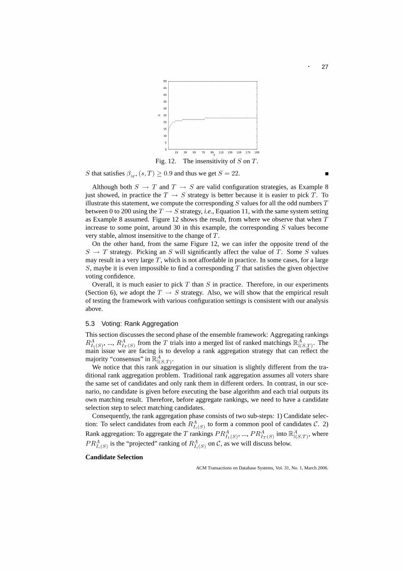
· 27

0

5

10

15

20

25

30

35

40

45

50

19 39 59 79 99 119 139 159 179 199

ST

Fig. 12. The insensitivity ofS onT .

S that satisfiesβM∗ (s, T ) ≥ 0.9 and thus we getS = 22.

Although bothS → T andT → S are valid configuration strategies, as Example 8just showed, in practice theT → S strategy is better because it is easier to pickT . Toillustrate this statement, we compute the correspondingS values for all the odd numbersTbetween 0 to 200 using theT → S strategy,i.e., Equation 11, with the same system settingas Example 8 assumed. Figure 12 shows the result, from where we observe that whenTincrease to some point, around 30 in this example, the correspondingS values becomevery stable, almost insensitive to the change ofT .

On the other hand, from the same Figure 12, we can infer the opposite trend of theS → T strategy. Picking anS will significantly affect the value ofT . SomeS valuesmay result in a very largeT , which is not affordable in practice. In some cases, for a largeS, maybe it is even impossible to find a correspondingT that satisfies the given objectivevoting confidence.

Overall, it is much easier to pickT thanS in practice. Therefore, in our experiments(Section 6), we adopt theT → S strategy. Also, we will show that the empirical resultof testing the framework with various configuration settings is consistent with our analysisabove.

5.3 Voting: Rank Aggregation

This section discusses the second phase of the ensemble framework: Aggregating rankingsRA

I1(S), ..., RAIT (S) from theT trials into a merged list of ranked matchingsRA

I(S,T ). Themain issue we are facing is to develop a rank aggregation strategy that can reflect themajority “consensus” inRA

I(S,T ).We notice that this rank aggregation in our situation is slightly different from the tra-

ditional rank aggregation problem. Traditional rank aggregation assumes all voters sharethe same set of candidates and only rank them in different orders. In contrast, in our sce-nario, no candidate is given before executing the base algorithm and each trial outputs itsown matching result. Therefore, before aggregate rankings, we need to have a candidateselection step to select matching candidates.

Consequently, the rank aggregation phase consists of two sub-steps: 1) Candidate selec-tion: To select candidates from eachRA

Ii(S) to form a common pool of candidatesC. 2)

Rank aggregation: To aggregate theT rankingsPRAI1(S), ...,PRA

IT (S) intoRAI(S,T ), where

PRAIi(S) is the “projected” ranking ofRA

Ii(S) onC, as we will discuss below.

Candidate Selection


28 ·We select candidates based on the intuition that if a matchingM is only discovered by

a minority of trials,M is more likely to be a false matching. Therefore, we consider amatching as a candidate if it appears in the majority ofT rankings,RA

I1(S), ...,RAIT (S). All

the matchings whose number of occurrences are less thanT+12 are thus pruned.

Let C denote the union of all the candidates in eachRAIi(S). After candidate selection,

we will remove the non-candidate matchings from eachRAIi(S) and meanwhile preserving

the ordering of candidates; the corresponding new ranked list, which can be viewed as a“projection” of RA

Ii(S) onC, contains only candidates and is denoted asPRAIi(S).

Example 9: Assume we execute the base algorithmA on three trials,i.e., T = 3, andthe outputs are thus three ranked listsRA

I1(S), RAI2(S) andRA

I3(S). SupposeRAI1(S) outputs

rankingM1 > M2 > M3 > M4 in descending order,RAI2(S) outputsM2 > M1 > M3 >

M5, andRAI3(S) outputsM3 > M1 > M2 > M4.

Since T+12 = 2, any matching that occurs only once will be pruned. In particular,M5

is pruned; other matchings,M1, M2, M3 andM4, all at least occur twice and thus areselected as matching candidates. Therefore, we haveC = {M1,M2,M3,M4}.

The projected rankings are thusRRAI1(S): M1 > M2 > M3 > M4, PRA

I2(S): M2 >

M1 > M3, andPRAI3(S): M3 > M1 > M2 > M4. In particular,M5 does not appear in

PRAI2(S) because it has been pruned.

Rank Aggregation

In rank aggregation, we need to construct an ordered listRAI(S,T ) for the candidates in

C, based on the individual ranksPRAI1(S), ...,PRA

IT (S). This problem is essentially arankaggregationproblem, which has been extensively studied as a particularvotingsystem inboth social science [Kemeny 1959; Young 1988] and computer science [Dwork et al. 2001;Fagin et al. 2003]. In the literature, many rank aggregation strategies have been proposed,such as Borda’s aggregation [Borda 1781], Kemeny optimal aggregation [Kemeny 1959],and footrule optimal aggregation [Dwork et al. 2001]. There does not exist an aggregationstrategy that can beat other strategies in all aspects– Different strategies have differentstrength and weakness.

Before discussing concrete aggregation strategies, we first need to solve the partial listproblem. Specifically, since the output of one trial may not contain all the candidates inC,PRA

Ii(S) may be only a partially ordered list. To be able to apply the aggregation strategy(as we will discuss below), it is necessary to also assign ranks to the candidates not inthe list. In our development, given a trial with a partial list, we assign all the uncoveredcandidates with the same lowest rank. Therefore, in one trial, a covered candidate is alwaysranked higher than an uncovered one, and two uncovered candidates are equally ranked.

Since essentially any rank aggregation strategy can be applied in our scenario, in our de-velopment, we test several different aggregation strategies and our goal is to find the mostappropriate one. We first choose the widely deployed Borda’s aggregation [Borda 1781] asthe baseline aggregation strategy. We then realize that to enforce the majority voting, it isimportant that an aggregation strategy satisfies theCondorcet criterion[Young 1988]. Wethus propose a strategy,FK aggregation, by combining Kemeny optimal aggregation [Ke-meny 1959] and footrule optimal aggregation [Dwork et al. 2001]. We will discuss thesetwo strategies,i.e., Borda’s aggregation and FK aggregation, in details respectively.


· 29

5.3.1 Baseline: Borda Aggregation.A primary strength of Borda’s aggregation is thatit is rather simple and computationally efficient: It can be implemented in linear time.Borda’s aggregation also satisfies some good properties such as anonymity, neutrality, andconsistency [Young 1974]. Specifically, in Borda’s aggregation, given a candidateMj ,let rji be the number of matchings ranked lower thanMj in PRA

Ii(S), theborda scoreof

Mj , denoted asB(Mj), is defined as the sum of allrji, i.e., B(Mj) =∑T

k=1 rjk. Theaggregation resultRA

I(S,T ) is thus the descending ordering of all the candidates with respectto their borda scores.

Example 10: Continue on Example 9, after candidate selection, we first complete the par-tial lists. In particular, sincePRA

I2(S) only partially ranks the four candidates, we assignthe lowest rank to the uncovered candidateM4, i.e., we rankM4 as the4th candidate inPRA

I2(S). Next, we compute the borda score for each candidate and then apply Borda’s

aggregation. In particular, sinceM1 is ranked higher than 3 candidates inPRAI1(S), 2

in PRAI2(S) and 2 inPRA

I3(S), the borda score forM1 is 3 + 2 + 2 = 7. Similarly, the

borda scores forM2 to M4 are 6, 5, 0 respectively. The final rankingRAI(S,T ) is thus

M1 > M2 > M3 > M4.

5.3.2 Enforcing Majority by Satisfying the Condorcet Criterion: FK Aggregation.Ouranalysis of the effectiveness of the ensembleDCM framework in Section 5.1 is basedon the assumption that when a matching is correctly ranked in the majority of trials, itwill be correctly ranked inRA

I(S,T ). Therefore, our aggregation strategy should reflect thisrequirement of majority– That is, if a matching can be correctly ranked in most trials, itsranking inRA

I(S,T ) should also be correct.We notice that this requirement is consistent with the classicCondorcet criterion[Young

1988]. Specifically, the Condorcet criterion requires that, given any two candidatesMi andMj , if a majority of trials ranksMi higher thanMj , thenMi should be ranked higher thanMj in the aggregate listRA

I(S,T ). (As we can see here, setting the number of trialsT asan odd number, as Section 5.1 discussed, can ensure that there will be no tie situationbetween any twoMi and Mj .) The fact that aggregation mechanisms that satisfy theCondorcet criterion can yield robust results has also been noticed and exploited by [Dworket al. 2001]. However, Borda’s aggregation, although computationally very fast, does notsatisfy the Condorcet criterion. To our knowledge, the only aggregation strategy exactlysatisfies the Condorcet criterion is Kemeny optimal aggregation. Another strategy, footruleoptimal aggregation, does not directly satisfy the Condorcet criterion, but its ordering ofmatchings yields a factor-2 approximation to Kemeny optimal aggregation.

Example 11: To see how Borda’s aggregation may not satisfy the Condorcet criterion, letus see an example, which is slightly different from Example 9. Assume after candidateselection, we haveRRA

I1(S): M1 > M2 > M3 > M4, PRAI2(S): M1 > M2 > M4 > M3,

andPRAI3(S): M2 > M3 > M4.

With Borda’s aggregation, we have the borda scores forM1, M2, M3 andM4 as 6, 7, 3,2 respectively. The ranking of matchings under Borda’s aggregation is thusM2 > M1 >M3 > M4. However,M1 is ranked higher thanM2 in the majority of trials,i.e., RRA

I1(S)

andRRAI2(S), which shows that Borda’s aggregation violates the Condorcet criterion and

therefore may not reflect the results of majority.

Although Kemeny optimal aggregation satisfies the Condorcet criterion, it is compu-


30 ·tationally expensive. Kemeny optimal aggregation is to find the ordered listRA

I(S,T ) that

minimizes∑T

i=1 K(PRAIi(S),R

AI(S,T )), whereK(PRA

Ii(S),RAI(S,T )) denotes theKendall

tau distance. That is, it is the number of pairs of candidates (Mi, Mj) on which the or-dered listsPRA

Ii(S) andRAI(S,T ) disagree (i.e., one ranksMi higher thanMj , while another

one ranksMj higher thanMi). It has been proven that computing Kemeny optimal ag-gregation is NP-Hard [Dwork et al. 2001], which is not affordable in practice. Hence, wecannot only apply this aggregation strategy.

As the approximation to Kemeny optimal aggregation, footrule optimal aggregation hasgood computational complexity. In footrule optimal aggregation, the aggregate listRA

I(S,T )

contains the median ranks of all the matchings. Specifically, given a candidateMj , letqji be the rank ofMj in PRA

Ii(S), themedian rankof Mi is defined asmedain(Mj) =median(qj1, ..., qjT ). The aggregation resultRA

I(S,T ) is thus the ordered list of medianranks of all the candidates. Footrule optimal aggregation can be computed in polynomialtime. Although it may not satisfy the Condorcet criterion, it has been shown that its order-ing of matchings (i.e., the footrule distance) has a factor-2 approximation to the Kendall taudistance in Kemeny optimal aggregation [Diaconis and Graham 1977]. However, footruleoptimal aggregation suffers the tie problem. That is, some matchings may have the samemedian rank and it is unclear how to break ties in footrule optimal aggregation.

Combining the strength of these two aggregation strategies, in our development, wedevelop a hybrid aggregation strategy,FK aggregation. In particular, we first apply footruleoptimal aggregation. To break a tie, we apply Kemeny optimal aggregation only locallyfor ranking the candidates that cause the tie. Empirically, since the number of candidatesresult in a tie is often very few (e.g., less than 4), the computation is very efficient.

Example 12: Let us apply FK aggregation for the case in Example 11. We first completethe partial lists. In particular, sincePRA

I3(S) only partially rank the four candidates, weassign the lowest rank to the uncovered candidateM1.

We then compute the median rank for each candidate and apply footrule optimal aggre-gation. In particular, the median rank forM1 is median(1, 1, 4) = 1. Similarly, the medianranks forM2 to M4 are 2, 3, 3 respectively.

SinceM3 andM4 get a tie in footrule optimal aggregation, we break the tie by ap-plying Kemeny optimal aggregation only onM3 andM4. Since two out of the three tri-als preferM3 thanM4, we rankM3 higher thanM4. The final rankingRA

I(S,T ) is thusM1 > M2 > M3 > M4, which is consistent with the result of only applying Kemenyoptimal aggregation, but more efficient.

6. EXPERIMENTS

We evaluate theDCM framework over real query interfaces. In particular, we implementall the algorithms in Python 2.4 and test all the experiments on a Windows XP machinewith Pentium M 1.6GHz CPU and 512M memory. We choose the TEL-8 dataset of theUIUC Web integration repository [Chang et al. 2003] as the testbed of both the baseDCMframework and the ensemble one. The TEL-8 dataset contains raw Web pages for 447 deepWeb sources in 8 popular domains, where each domain has about 20-70 sources.

Experiment SuitesTo evaluate the performance of the algorithms we have developed in this article, we

design two suites of experiments. The first suite of experiments is to evaluate the effec-


· 31

tiveness of the baseDCM framework by testing it on manually extracted interfaces. Ourgoal is to isolate the matching process to study and thus fairly evaluate its performance. Inparticular, we assume a perfect interface extractor to extract all the interfaces in the TEL-8dataset into query capabilities by manually doing the extraction work. After extracting theraw data, we do the data preprocessing according to the process explained in Section 3.3.Then, we run the dual correlation mining and matching construction algorithms on the pre-processed data in each domain. In the results, we use attribute name and type together asthe attribute identifier for an attribute entity since we incorporate the type recognition stepto identify homonyms (Section 3.3). The experimental result shows that the baseDCMframework achieves goodtarget accuracyon manually extracted schemas. We also evalu-ate the effectiveness of the matching selection algorithm and the data preprocessing step.Further, we compare theH-measure with other measures on the same dataset and the resultshows thatH-measure outperforms the others in most cases. Section 6.1 will report theseresults.

The second suite of experiments is to verify the impact of noises in the interface extrac-tion on our matching algorithm and evaluate the performance of the ensemble approach.In particular, we conduct our evaluations on automatically extracted interfaces in two do-mains: Books and Airfares. First, we directly run the baseDCM framework on automati-cally extracted interfaces as the baseline result that we will compare to. Second, we mea-sure the accuracy of the ensembleDCM framework and compare it to the baseline result.The experiments show that the ensemble approach can significantly improve the matchingaccuracy ofDCM. Third, we execute the ensembleDCM framework under various para-meter settings and compare the empirical values with our theoretical analysis. Section 6.2will report these results.

Note that, to illustrate the effectiveness of the dual correlation mining, we only list andcount the “semantically difficult” matchings discovered by the mining algorithm, not thesimple matchings by the syntactic merging in the data preprocessing (e.g., merging “titleof book” to “title”). Our experiment shows that many frequently observed matchings arein fact “semantically difficult” and thus cannot be found by syntactic merging.

MetricsWe compare experimentally discovered matchings, denoted byMh, with correct match-

ings written by human experts, denoted byMc. In particular, we adopt thetarget accuracy,a metric initially developed in [He and Chang 2003], by customizing thetarget questionsto the complex matching scenario. The idea of the target accuracy is to measure how accu-rately the discovered matchings answer the target questions. Specifically, for our complexmatching task, we consider the target question as, given any attribute, to find its synonyms(i.e., word with exactly the same meaning as another word,e.g., subject is a synonym ofcategory in the Books domain), hyponyms (i.e., word of more specific meaning,e.g., lastname is a hyponym ofauthor) and hypernyms (i.e., word with a broader meaning, e.g,author is a hypernym oflast name).

It is quite complicated to use different measures for different semantic relationships, wetherefore report an aggregate measure for simplicity and, at the same time, still reflectingsemantic differences. For our discussion here, we name synonym, hyponym and hypernymtogether asclosenym– meaning that they all denote some degrees of closeness in semanticmeanings. Our target question now is to ask the set of closenyms of a given attribute.

Example 13: For instance, for matching{A} = {B, C}, the closenym sets of attributesA,


32 ·Step Value of Result Cmin Cmax

group G G1 = {last name (unknown),first name (any)} 0.94discovery G2 = {title (any),keyword (any)} 0.93

G3 = {last name (any),title (any)} 0.91G4 = {first name (any),catalog (any)} 0.90G5 = {first name (any),keyword (any)} 0.87

matching R M1: {author (any)} = {last name (any),first name (any)} 0.87 0.87discovery M2: {author (any)} = {last name (any)} 0.87 0.87

M3: {subject (string)} = {category (string)} 0.83 0.83M4: {author (any)} = {last name (any),catalog (any)} 0.82 0.82M5: {author (any)} = {first name (any)} 0.82 0.82M6: {category (string)} = {publisher (string)} 0.76 0.76

matching {author (any)} = {last name (any),first name (any)} 0.87selection {subject (string)} = {category (string)} 0.83

Fig. 13. Running dual correlation mining and matching construction on the Books domain.

B, C are{B, C}, {A}, {A} respectively. In particular, the closenym sets ofB does not haveC sinceB andC only have grouping relationship. In contrast, for matching{A} = {B} ={C}, the closenym sets of attributesA, B, C are{B, C}, {A, C}, {A, C} respectively. Wecan see that the difference of matchings can be reflected in the corresponding closenymsets.

Except this difference in target question, we use the same metric of target accuracyas [He and Chang 2003]. Specifically, we assume a “random querier” to ask for theclosenym set of each attribute according to its frequency. The answer to each question isthe closenym set of the queried attribute in discovered matchings. We defineCls(Aj |M)as the closenym set of attributeAj . GivenMc andMh, the precision and recall of theclosenym sets of attributeAj are:

PAj (Mh,Mc) = |Cls(Aj |Mc)∩Cls(Aj |Mh)||Cls(Aj |Mh)| and

RAj (Mh,Mc) = |Cls(Aj |Mc)∩Cls(Aj |Mh)||Cls(Aj |Mc)| .

Since more frequently used attributes have higher probabilities to be asked in this “ran-dom querier,” we compute the weighted average of all thePAj ’s andRAj ’s as thetarget

precisionandtarget recall. The weight is assigned asOjPOk

, whereOj is the frequency ofattributeAj in the dataset (i.e., its number of occurrences in different schemas). Therefore,target precisionandtarget recallof Mh with respect toMc are:

PT (Mh,Mc) =∑

Aj

OjPOk

PAj (Mh,Mc)

RT (Mh,Mc) =∑

Aj

OjPOk

RAj (Mh,Mc).

6.1 Base DCM Framework

In this subsection, we report the first suite of experiment: The evaluation of the baseDCMframework.

Result on the TEL-8 dataset: In this experiment, we run our algorithm (withH-measureas the correlation measure) on manually extracted TEL-8 dataset. We set the thresholdsTp

to 0.85 andTd to 0.6 for positive correlation mining andTn to 0.75 for negative correlationmining. We empirically get these numbers by testing the algorithm with various thresh-olds and choose the best one in the Books domain. As we discussed in Section 4.2, thereason we do not need to consider the number of input schemas in the parameter setting is


· 33

Domain Final Output After Matching Selection Correct?Airfares {destination (string)} = {to (string)} = {arrival city (string)} Y

{departure date (datetime)} = {depart (datetime)} Y{passenger (integer)} = {adult (integer),child (integer),infant (integer)} P{from (string),to (string)} = {departure city (string),arrival city (string)} Y{from (string)} = {depart (string)} Y{return date (datetime)} = {return (datetime)} Y

Movies {artist (any)} = {actor (any)} = {star (any)} Y{genre (string)} = {category (string)} Y{cast & crew (any)} = {actor (any),director (any)} Y

MusicRecords title (unknown) =album (unknown) Ykeyword (unknown) ={song (unknown), album (unknown)} Ngenre (string) =category (string) Y

Hotels {check in (date),check out (date)} = Y{check in date (date),check out date (date)}check in (date) =check in date (date) Ycheck out (date) =check out date (date) Ytype (string) =country (string) Nguest (integer) ={adult (integer),child (integer),night (integer)} P

Fig. 14. Experimental results for Airfares and Movies.

thatH-measure satisfies the sampling invariance property. We then observe that differentdomains often have similar popularity and occurrence behavior of attributes, as our deepWeb survey [Chang et al. 2004] studies. Therefore, we reuse the setting of parametersin the Books domain for all the other domains in both the baseDCM and the ensembleDCM frameworks. The sampling invariance property ofH-measure and the observationof attribute distribution similarity across domains greatly alleviate our effort on parametertuning for developing an automatic query interface matcher for various sampling sizes anddifferent domains.

Figure 13 illustrates the detailed results ofn-ary complex matchings discovered in theBooks domain. The step of group discovery found 5 likely groups (G1 to G5 in Figure 13).In particular,mp gives a high value (actually the highest value) for the group oflast name(any) andfirst name (any). The matching discovery found 6 likely complex matching (M1

to M6 in Figure 13). We can see thatM1 andM3 are fully correct matchings, while othersare partially correct or incorrect. Last, the matching construction will chooseM1 andM3

(i.e., the correct ones) as the final output.Figure 14 shows the results of some other domains,i.e., Airfares, Movies, Music Records

and Hotels. The third column denotes the correctness of the matching. In particular,Ymeans a fully correct matching,P a partially correct one andN an incorrect one. Ourmining algorithm does find interesting matchings in almost every domain. For instance, inthe Airfares domain, we find 5 fully correct matchings,e.g., {destination (string)} = {to(string)} = {arrival city (string)}. Also, {passenger (integer)} = {adult (integer),child(integer),infant (integer)} is partially correct because it missessenior (integer).

Since, as a statistical method, our approach replies on “sufficient observations” of at-tribute occurrences, it is likely to perform more favorably for frequent attributes (i.e., thehead-ranked attributes in Figure 8). To quantify this “observation” factor, we report thetarget accuracy with respect to the attribute frequencies. In particular, we consider theattributes above afrequency thresholdF (i.e., the number of occurrences of the attributeover the total number of schemas is aboveF ) in both discovered matchings and correctmatchings to measure the target accuracy. Specifically, we run the algorithms on all the


34 ·Domain PT RT PT RT

(20%) (20%) (10%) (10%)Books 1 1 1 1Airfares 1 1 1 0.71Movies 1 1 1 1MusicRecords 1 1 0.76 1Hotels 0.86 1 0.86 0.87CarRentals 0.72 1 0.72 0.60Jobs 1 0.86 0.78 0.87Automobiles 1 1 0.93 1

Fig. 15. Target accuracy of the 8 domains.

Domain reduced missed reduced missedfalse positive false positive false positive false positive

(20%) (20%) (10%) (10%)Books 0 0 3 0Airfares 2 0 22 0Movies 0 0 2 0MusicRecords 3 0 5 1Hotels 6 1 11 2CarRentals 2 1 2 1Jobs 4 0 9 1Automobiles 0 0 2 1

Fig. 16. The effectiveness of reducing false matchings in the matching selection step.

attributes and then report the target accuracy in terms of the frequency-divided attributes.In the experiment, we chooseF as 20% and 10%.

Consider the Airfares domain, if we only consider the attributes above 20% frequency inthe matching result, only 12 attributes are above that threshold. The discovered matchingsin Figure 14 become{destination (string)} = {to (string)}, {departure date (datetime)}= {depart (datetime)}, and{return date (datetime) =return (datetime)}. (The otherattributes are removed since they are all below 20% frequency.) These three matchings areexactly the correct matchings the human expert can recognize among the 12 attributes andthus we get 1.0 in both target precision and recall.

Next, we apply the 10% frequency threshold and get 22 attributes. The discoveredmatchings in Figure 14 are unchanged since all the attributes (in the matchings) are nowpassing the threshold. Compared with the correct matchings among the 22 attributes, we domiss some matchings such as{cabin (string)} = {class (string)} and{departure (date-time) = departure date (datetime)}. Also, some matchings are partially correct such as{passenger (integer)} = {adult (integer),child (integer),infant (integer)}. Hence, we get1.0 in target precision and 0.71 in target recall.

Figure 15 lists the target accuracies of the 8 domains under thresholds 20% and 10%.From the result, we can see that our approach does perform better for frequent attributes.

Evaluating the Matching Selection Strategy: To evaluate the effectiveness of the match-ing selection algorithm we developed in Section 3.2, which exploits conflict betweenmatching candidates to remove false positives, we count the number of false matchings


· 35

Domain PT RT PT RT

(20%) (20%) (10%) (10%)Books 0.79(-0.21) 1 0.74(-0.26) 1Airfares 1 1 0.81(-0.19) 0.82(+0.11)Movies 1 1 0.87(-0.13) 1MusicRecords 0.93(-0.07) 1 0.70(-0.06) 1Hotels 0.66(-0.20) 1 0.47(-0.39) 0.46(-0.41)CarRentals 1 (+0.28) 0.63(-0.37) 1 (+0.28) 0.16(-0.44)Jobs 0.70(-0.30) 1 (+0.14) 0.52(-0.26) 0.87Automobiles 1 1 0.66(-0.27) 0.68(-0.32)

Fig. 17. Target accuracy of the 8 domains without data preprocessing.

reduced and missed by the selection step respectively. Figure 16 lists this result for theeight domains under both 20% and 10% frequency thresholds. We can see that the greedyselection strategy based onCmax measure is quite effective in reducing false matchings.Most false matchings are removed in the selection step. In particular, although the 10%frequency threshold may result in more false matchings comparing to the 20% one, theselection strategy can remove most of them and keep the performance good. For instance,in the Airfares domain under 10% frequency threshold, 22 false matchings are removedand no false matching is missed.

Evaluating the Data Preprocessing Step: To evaluate the effectiveness of the data pre-processing step, we test theDCM algorithm over schemas without data preprocessing. Inparticular, we only perform the standard normalization sub-step in Section 3.3 for the inputschemas and ignore the type recognition and syntactic merging sub-steps. Our goal is tosee the impact of these sub-steps on the accuracy of matching.

Intuitively, although query interfaces are quite concerted in terms of the attributes theyuse, there still are many syntactic variations for expressing the same attribute,e.g., title,book title, title of book and search by title for attribute “title.” As discussed in Sec-tion 3.3, type recognition and syntactic merging can help merge these variations into asingle attribute and thus increase attribute occurrences across query interfaces, which canimprove the performance of the subsequent correlation mining algorithm.

Figure 17 shows the result of running theDCM algorithm with non-preprocessed schemasas input. In Figure 17, we write accuracies that change after removing the data preprocess-ing step in italic font and show the differences in brackets. As we can see, the accuraciesfor many domains are much worse than the ones with data preprocessing in Figure 15.In particular, under the 10% frequency threshold, where more attributes are consideredfor mining matchings, accuracies are greatly reduced. Therefore, applying the data pre-processing step, although may itself result in some errors, is crucial for our mining-basedmatching approach and can indeed significantly enhance the matching accuracy.

Evaluating the H-measure: We compare theH-measure with other measures and theresult shows that theH-measure gets better target accuracy. As an example, we chooseJaccard(ζ) as the measure we compare to. WithJaccard, we define themp andmn as

mp(Ap, Aq) ={

ζ(Ap, Aq), f11f++

< Td

0, otherwise,

and


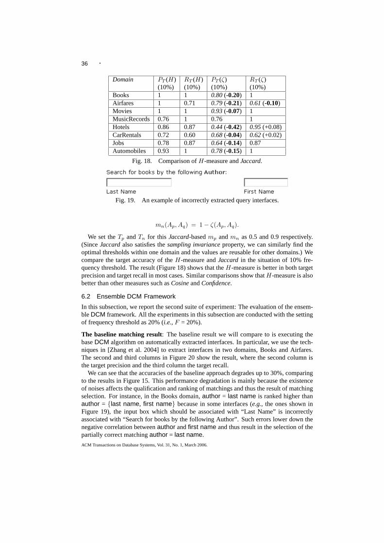
36 ·Domain PT (H) RT (H) PT (ζ) RT (ζ)

(10%) (10%) (10%) (10%)Books 1 1 0.80(-0.20) 1Airfares 1 0.71 0.79(-0.21) 0.61(-0.10)Movies 1 1 0.93(-0.07) 1MusicRecords 0.76 1 0.76 1Hotels 0.86 0.87 0.44(-0.42) 0.95(+0.08)CarRentals 0.72 0.60 0.68(-0.04) 0.62(+0.02)Jobs 0.78 0.87 0.64(-0.14) 0.87Automobiles 0.93 1 0.78(-0.15) 1

Fig. 18. Comparison ofH-measure andJaccard.

Fig. 19. An example of incorrectly extracted query interfaces.

mn(Ap, Aq) = 1− ζ(Ap, Aq).

We set theTp andTn for this Jaccard-basedmp andmn as 0.5 and 0.9 respectively.(SinceJaccardalso satisfies thesampling invarianceproperty, we can similarly find theoptimal thresholds within one domain and the values are reusable for other domains.) Wecompare the target accuracy of theH-measure andJaccard in the situation of 10% fre-quency threshold. The result (Figure 18) shows that theH-measure is better in both targetprecision and target recall in most cases. Similar comparisons show thatH-measure is alsobetter than other measures such asCosineandConfidence.

6.2 Ensemble DCM Framework

In this subsection, we report the second suite of experiment: The evaluation of the ensem-bleDCM framework. All the experiments in this subsection are conducted with the settingof frequency threshold as 20% (i.e., F = 20%).

The baseline matching result: The baseline result we will compare to is executing thebaseDCM algorithm on automatically extracted interfaces. In particular, we use the tech-niques in [Zhang et al. 2004] to extract interfaces in two domains, Books and Airfares.The second and third columns in Figure 20 show the result, where the second column isthe target precision and the third column the target recall.

We can see that the accuracies of the baseline approach degrades up to 30%, comparingto the results in Figure 15. This performance degradation is mainly because the existenceof noises affects the qualification and ranking of matchings and thus the result of matchingselection. For instance, in the Books domain,author = last name is ranked higher thanauthor = {last name, first name} because in some interfaces (e.g., the ones shown inFigure 19), the input box which should be associated with “Last Name” is incorrectlyassociated with “Search for books by the following Author”. Such errors lower down thenegative correlation betweenauthor andfirst name and thus result in the selection of thepartially correct matchingauthor = last name.


· 37

Domain The base The ensembleDCM framework The ensembleDCM frameworkDCM framework with Borda’s aggregation with FK aggregationPT RT PAT RAT PFT RFT PAT RAT PFT RFT

Books 0.73 0.75 0.83 0.89 0.9 1.0 0.83 0.9 0.9 1.0Airfares 0.67 0.68 0.79 0.79 0.71 0.82 0.91 0.73 1.0 0.73

Fig. 20. The comparison of target accuracy on Books and Airfares.

Also, due to the greedy selection strategy, the errors caused in one iteration may cascadeto its subsequent iterations. For instance, still in the Books domain, whenauthor = {lastname, first name} is pruned out (because of the above reason), in the next iteration ofselection,isbn = {last name, first name} is selected as a correct matching, which makesthe result even worse.

The performance of the ensembleDCM framework : Before running the ensembleframework, we need to first determine its configuration. In our experiment, we choosetheT → S configuration strategy developed in Section 5.2. Specifically, we set the num-ber of trialsT as 41 and objective voting confidencec as 0.9 for both Books and Airfares.(As we modeled in Section 5.1,T is set as an odd number. We have no particular reasonfor choosing 41. As Section 5.2 discussed,S is insensitive toT and thus picking otherTvalues will not significantly affect the final performance. We also empirically verify thisfact later.) We then setW ∗ andK∗ values according to our estimation strategy of the baseparameters. In particular, for Books, we haveW ∗ = 6 and for Airfares,W ∗ = 5. For bothdomains, we setK∗ as a small constant 2. Thus, according to Equation 11, we haveS= 22 for Books andS = 19 for Airfares. Also, for each dataset, we test it with the twoaggregation strategies we developed in Section 5.3 respectively: The Borda’s aggregationand the FK aggregation.

As the ensemble framework is essentially a data-randomized approach (with multiplerandom trials), it is “non-deterministic”– We thus measure the distribution of its perfor-mance. Specifically, we execute the framework 100 times on Books with the same settingS = 22,T = 41. Similarly, we execute it 100 times on Airfares with the same settingS =19,T = 41. To quantify the comparison with the baseline result, we measure two suites oftarget accuracies: theaverage target accuracy(i.e., the average precision and recall of the100 executions, denoted asPAT andRAT respectively) and themost frequent target accu-racy (i.e., the most frequently obtained precision and recall of the 100 executions, denotedasPFT andRFT respectively). Note that we do not use the best target accuracy (i.e., thebest precision and recall of the 100 executions) as we did in [He and Chang 2005] becausein practice we cannot judge which result is the best without knowledge from human ex-perts. In contrast, most frequent accuracy is more meaningful since it can be obtained byexecuting the ensemble framework multiple times and taking their majority.

The results of both average and most frequent accuracies are listed in Figure 20 (columns3-6 for Borda’s aggregation and columns 7-10 for FK aggregation). We can see that: 1)Comparing to the baseline result, precision and recall are improved by the ensemble frame-work under both aggregation strategies. 2) For the Books domain, Borda’s aggregation andFK aggregation have roughly the same accuracy; For the Airfares domain, FK aggregationcan achieve much higher precision than Borda’s aggregation, but with slightly lower recall.

Overall, the ensemble framework is quite effective in maintaining the robustness of theDCM matcher. The FK aggregation strategy can yield more robust results than Borda’saggregation. We believe this experiment shows that, while Borda is actually a reasonable


38 ·

(a) Books. (b) Airfares.Fig. 21. The target precision with 100 executions on two domains (Borda’s aggregation).

(a) Books. (b) Airfares.Fig. 22. The target recall with 100 executions on two domains (Borda’s aggregation).

(a) Books. (b) Airfares.Fig. 23. The target precision with 100 executions on two domains (FK aggregation).

baseline choice, FK is indeed more robust. Next, we illustrate and interpret the results ofthe ensemble framework with more details.

First, in most executions, the ensemble framework achieves better accuracy than thebaseline result. For instance, Figure 21 shows the 100 target precisions of the 100 ex-ecutions over Books and Airfares with Borda’s aggregation. To make Figure 21 moreillustrative, we use straight horizontal lines to denote the baseline accuracies. We can see


· 39

(a) Books. (b) Airfares.Fig. 24. The target recall with 100 executions on two domains (FK aggregation).

that, although accuracies may be varying in different executions, most precisions in bothBooks and Airfares are better than their corresponding baseline precisions. Similar resultcan also be observed in the target recall part (Figure 22) under Borda’s aggregation andboth precision (Figure 24) and recall (Figure 24) under FK aggregation. Hence, this ex-periment indicates that the ensemble framework can indeed boost the matching accuracyunder noisy schema input, and thus maintain the desired robustness of a holistic matcher.Note that the recall graphs looks more regular than the precision ones because for recall,only the value on numerator is changing, while for precision, values on both numeratorand denominator are changing.

Second, from Figures 21 to 24, we also observe an interesting phenomenon: It seemsthat there are upper-bounds for both precision and recall, which the ensemble frameworkcannot exceed. The existence of such upper bounds is because, in essence, there are twotypes of data quality problems, noises and missing data, and the ensemble frameworkcan deal with noises, but not missing data. Specifically, noises are some observed datathat ideally should not be observed,i.e., outliers. For instance, the extraction of a bookschema,e.g., the one in Figure 19, may incorrectly consider “author” as an attribute andthus lowers down the correlation of “author” and “first name.” Although noises may affectthe accuracy of the base algorithm, they are minority in quantity. Downsampling is thus agood approach to filtering them out and, consequently, the majority voting can be effective.On the other hand,missing dataare some data that ideally should be observed, but in realityare not. For instance, the input schemas may contain only a small number of occurrencesof the attribute “last name” and thus we cannot sufficiently identify to find the grouping of“last name” and “first name.” For this missing data case, sampling and voting techniqueswill not help, since when the entire dataset has missing data, all the trials will also havemissing data and their aggregate result cannot fix the problem. The ensemble framework,with the limit imposed by such missing data, has an upper bound for the best accuracy.

Finally, the execution time of the ensemble framework is also acceptable. The 100executions on Books take 118 seconds for Borda’s aggregation and 117 seconds for FKaggregation. The 100 executions on Airfares take 109 seconds for Borda’s aggregation and128 seconds for FK aggregation. Therefore, the average time for one execution is aboutonly 1 second.

The result under various configuration settings:The purpose of this set of experiments


40 ·

0

0.2

0.4

0.6

0.8

1

10 15 20 25 30 35 40 45 50 55

Acc

urac

y

Sampling Size S

Target PrecisionTarget Recall

Target F

0

0.2

0.4

0.6

0.8

1

10 13 16 19 22 25 28 31 34 37 40

Acc

urac

y

Sampling Size S


Target F

(a) Books (T=41). (b) Airfares (T=41).

Fig. 25. The target accuracy under various sampling sizes (Borda’s aggregation).

is to empirically verify our analysis in Section 5.2: 1) We want to verify whether oursetting ofS using Equation 11 is consistent with empirical observation. 2) We want toverify whether the performance of the framework is indeed insensitive toT , but sensitiveto S.

First, we measure the accuracy of the ensemble framework with different sampling sizeson the two domains. In particular, we fixT at 41 and letS progressively increase from10 to 55 with an increment size 5 (i.e., 10, 15, 20, ..., 55) for Books and from 10 to 40with an increment size 3 for Airfares. For each sampling size, we execute the ensembleframework 30 times under the two aggregation strategies respectively and compute theaverage precisions and recalls. Figure 25 shows the experimental result under Borda’saggregation and Figure 26 FK aggregation.

From Figures 25 and 26, we can observe the same trend in both domains, which seemsto be independent of the aggregation strategy we choose. Specifically, when samplingsize increases, the target precision mostly keeps on decreasing, while the target recall goesup first and then goes down at some point. We give the explanation as below: A smallsampling size may miss some attributes in downsampling and thus discover less matchings,which results in trivially high precision but low recall. With larger sampling size, we areable to cover more attributes and thus discover not only more correct matchings, but alsoa few false matchings. Consequently, the precision decreases and recall increases. Whenthe sampling size is too large, a downsampling is likely to have many noises and thus therecall starts to decrease again.

The best sampling size we should take is thus some values in the middle. We choose theF -measure, which combines precisionP and recallR asF = 2PR

P+R , to measure the overallaccuracy. From Figure 25(a) and Figure 26(a), we can see the best range of sampling sizefor Books, according toF -measure, is around 20. Our setting based on Equation 11 is 22,which is quite close to 20. Similarly, from Figure 25(b) and Figure 26(b), the best rangeof sampling size for Airfares is around 16. Our setting based on Equation 10 is 19, whichis also close. Therefore, our configuration strategy of determining the sampling size isconsistent with the empirical result.

Second, since we chooseT as 41 with no particular reason in the experiment, we wantto verify that the choosing otherT values is in fact not quite different, because of theinsensitivity ofS on T (Section 5.2). In particular, we fixS at 22 for Books and 19 forAirfares. We changeT from 5 to 49 with increment size 4 for both domains. For eachT ,


· 41

0

0.2

0.4

0.6

0.8

1

10 15 20 25 30 35 40 45 50 55

Acc

urac

y

Sampling Size S


Target F

0

0.2

0.4

0.6

0.8

1

10 13 16 19 22 25 28 31 34 37 40

Acc

urac

y

Sampling Size S


Target F

(a) Books (T=41). (b) Airfares (T=41).

Fig. 26. The target accuracy under various sampling sizes (FK aggregation).

0.1

0.2

0.3

0.4

0.5

0.6

0.7

0.8

0.9

1.0

5 9 13 17 21 25 29 33 37 41 45 49

Acc

urac

y

Number of Trials T


0.1

0.2

0.3

0.4

0.5

0.6

0.7

0.8

0.9

1.0

5 9 13 17 21 25 29 33 37 41 45 49

Acc

urac

y

Number of Trials T


(a) Books (S=22). (b) Airfares (S=19).

Fig. 27. The target accuracy under various number of trials (Borda’s aggregation).

we again execute the framework 30 times under the two aggregation strategies and computethe average precisions and recalls. Figures 27 and 28 shows the experimental results. Fromthe results, we can see that, in both domains, both the precision and recall become moreand more flat and stable whenT increases. This result indicates that with otherT values(as long as it is not too small), we can also have roughly the same performance and thusthe decision onT is not a critical factor.

Also, comparing Figure 27 and Figure 28, we can observe that the ensemble framworkwith FK aggregation generally can achieve better precision than the one with Borda’s ag-gregation. This result indicates that FK aggregation is more robust than Borda’s aggrega-tion in dealing with noisy data, since it approximates the Condorcet criterion (Section 5.3).

Overall, from these two experiments onS andT , we can see that under the sameT ,different sampling sizesS will significantly affect the performance of the data-ensembleframework, while on the other hand, under the sameS, different number of trialsT havelittle impact on the performance. This sensitivity of performance onS but notT indicatesthat theT → S configuration strategy is better thanS → T becauseT is much easier topick in practice, which verifies our analysis in Section 5.2.


42 ·

0

0.2

0.4

0.6

0.8

1

5 9 13 17 21 25 29 33 37 41 45 49

Acc

urac

y

Number of Trials T


0

0.2

0.4

0.6

0.8

1

5 9 13 17 21 25 29 33 37 41 45 49

Acc

urac

y

Number of Trials T


(a) Books (S=22). (b) Airfares (S=19).

Fig. 28. The target accuracy under various number of trials (FK aggregation).

7. RELATED WORK

We relate our work to the literature in two aspects: theproblemand ourtechniques. Inparticular, in terms of the problem, we discuss the difference of our work with 1) tradi-tional schema matching works; 2) recent works on matching Web databases. In terms ofour techniques, we discuss the distinctions of 1) our mining techniques; 2) our ensemblematching approach.

First, in terms of theproblem: Schema matching is important for schema integra-tion [Batini et al. 1986; Seligman et al. 2002] and thus has got great attention. However,existing schema matching works mostly focus on simple 1:1 matching [Rahm and Bern-stein 2001; Doan et al. 2001; Madhavan et al. 2001] between two schemas. Complexmatching has not been extensively studied, mainly due to the much more complex searchspace of exploring all possible combinations of attributes. Consider two schemas withuandv attributes respectively, while there are onlyu×v potential 1:1 matchings, the numberof possiblem:n matchings is exponential. A recent work iMAP [Dhamankar et al. 2004]proposes to construct 1:n matchings between two schemas by combining their simple 1:1matchings. Although both aiming at complex matchings, our work is different from iMAPin: 1) scenario: iMAP focuses on matching two schemas, while we targets at large scaleschema matching. 2)techniques: iMAP relies on the availability of instance values to con-struct complex matchings from simple 1:1 matchings, while we explore the co-occurrenceinformation across schemas and thus develop a correlation mining approach.

Some recent works are particularly focusing on matching Web databases [He et al. 2003;Wu et al. 2004; Wang et al. 2004]. WISE [He et al. 2003] is a comprehensive query inter-face integrator, which evaluates the similarity of attributes in multiple aspects. However, itonly deals with simple 1:1 matchings. Reference [Wang et al. 2004] matches query inter-faces based on the results of probing some instance values from the back-end databases viainterfaces. It also only deals with simple 1:1 matchings. Comparing with other matchingapproaches, probing-based matching is much more expensive due to the large number ofHTTP requests sent for each interface. In addition, it needs global model for each domainand thus less scalable as an automatic generic solution for handling various domains ofWeb sources. Reference [Wu et al. 2004] pursues a clustering-based approach to discover1:n matchings by exploring the “bridging” effect among query interfaces. However, its dis-covery of complex matchings essentially depends on a “hierarchical” interface extractor–


· 43

That is, the grouping of attributes (e.g., the grouping oflast name andfirst name) mustbe identified, in the first place, by the interface extractor (and not the matching algorithm).This “hierarchy-recognition” requirement makes interface extraction a very challengingtask. In contrast, theDCM framework only requires an interface extractor to extract a queryinterface as a “flat” set of query conditions, instead of a hierarchy of attributes, which canthus be easily satisfied (e.g., our recent work of automatic interface extraction [Zhang et al.2004] is such an extractor). In fact, even with a simple “flat” extractor, it already introducesenough errors to impact the matching performance. In this article, we study such impactand propose an ensemble approach for maintaining the robustness of matching, which sig-nificantly extends theDCM framework (Figure 2), as described in our earlier work [Heet al. 2004].

Our previous schema matching work, theMGS framework [He and Chang 2003], alsomatches Web interfaces by exploiting holistic information. Although built upon the sameinsight,DCM is different fromMGS in: 1) abstraction: DCM abstracts schema matchingas correlation mining, whileMGS as hidden model discovery by applying statistical hy-pothesis testing. The difference in abstraction leads to fundamentally different approaches.2) expressiveness: DCM findsm:n matchings, whileMGS currently finds 1:1 matchingsand it is unclear that how it can be extended to supportm:n matchings.

Second, in terms of ourtechniques: In this article, we propose a correlation mining viewfor the schema matching problem. Unlike previous correlation mining algorithms, whichmainly focus on finding strong positive correlations [Agrawal et al. 1993; Tan et al. 2002;Omiecinski 2003; Lee et al. 2003; Brin et al. 1997], our algorithm cares not only positivebut also negative correlations. In particular, as a new application for correlation mining, thecorrectness of schema matching mainly depends on the subtlety of negative correlations.We thus study the rare attribute problem and develop theH-measure, which empiricallyoutperforms existing ones on evaluating negative correlations.

In addition, as discussed in Section 5, our ensemble idea is inspired bagging classi-fiers [Breiman 1996]. However, our approach is different from bagging classifiers in threeaspects: The setting, the techniques and the analytical modeling.

8. CONCLUSION

This article explores co-occurrence patterns among attributes to tackle the complex match-ing problem. This exploration is well suited for the integration of large-scale heteroge-nous data sources, such as the deep Web. Specifically, we abstract complex matching ascorrelation mining and develop theDCM framework. Unlike previous correlation miningalgorithms, which mainly focus on finding strong positive correlations, our algorithm caresboth positive and negative correlations, especially the subtlety of negative correlations, dueto its special importance in schema matching. This difference leads to the introduction ofa new correlation measure,H-measure, distinct from those proposed in previous work.Further, when connecting theDCM framework with automatic interface extractor to fullyautomate the matching process, we notice that noises in the interface extraction may sig-nificantly affect the matching result. To make theDCM framework robust against noisyschemas, we integrate it with an ensemble scheme by exploiting statistical sampling andvoting. Our experiments validate the effectiveness of the correlation mining algorithm, theH-measure and the ensembleDCM framework.


44 ·REFERENCES

AGRAWAL , R., IMIELINSKI , T., AND SWAMI , A. N. 1993. Mining association rules between sets of items inlarge databases. InSIGMOD 1993 Conference.

ANDERSON, D. R., SWEENEY, D. J., AND WILLIAMS , T. A. 1984. Statistics for Business and Economics(Second Edition). West Pub. Co.

BATINI , C., LENZERINI, M., AND NAVATHE , S. B.1986. A comparative analysis of methodologies for databaseschema integration.ACM Computing Surveys 18,4, 323–364.

BERGMAN, M. K. 2000. The deep web: Surfacing hidden value. Tech. rep., BrightPlanet LLC. Dec.

BORDA, J. C.1781. Memoire sur leselections au scrutin.Histoire de l’Academie Royale des Sciences.

BREIMAN , L. 1996. Bagging predictors.Machine Learning 24,2, 123–140.

BRIN, S., MOTWANI , R., AND SILVERSTEIN, C. 1997. Beyond market baskets: generalizing association rulesto correlations. InSIGMOD 1997 Conference.

BRUNK, H. D. 1965.An Introduction to Mathematical Statistics. New York, Blaisdell Pub. Co.

CHANG, K. C.-C., HE, B., L I , C., PATEL , M., AND ZHANG, Z. 2004. Structured databases on the web:Observations and implications.SIGMOD Record 33,3, 61–70.

CHANG, K. C.-C., HE, B., L I , C., AND ZHANG, Z. 2003. The UIUC web integration repository. ComputerScience Department, University of Illinois at Urbana-Champaign. http://metaquerier.cs.uiuc.edu/repository.

CHANG, K. C.-C., HE, B., AND ZHANG, Z. 2005. Toward large scale integration: Building a metaquerier overdatabases on the web. InCIDR 2005 Conference.

CHAUDHURI , S., GANJAM , K., GANTI , V., AND MOTWANI , R. 2003. Robust and efficient fuzzy match foronline data cleaning. InSIGMOD 2003 Conference.

DHAMANKAR , R., LEE, Y., DOAN, A., HALEVY, A., AND DOMINGOS, P.2004. imap: Discovering complexsemantic matches between database schemas. InSIGMOD 2004 Conference.

DIACONIS, P. AND GRAHAM , R. 1977. Spearman’s footrule as a measure of disarray.Journal of the RoyalStatistical Society, Series B 39,2, 262–268.

DOAN, A., DOMINGOS, P., AND HALEVY, A. Y. 2001. Reconciling schemas of disparate data sources: Amachine-learning approach. InSIGMOD 2001 Conference.

DWORK, C., KUMAR , R., NAOR, M., AND SIVAKUMAR , D. 2001. Rank aggregation methods for the web. InWWW 2001 Conference.

FAGIN , R., KUMAR , R., AND SIVAKUMAR , D. 2003. Efficient similarity search and classification via rankaggregation. InSIGMOD 2003 Conference.

GOODMAN, L. AND KRUSKAL, W. 1979. Measures of Association for Cross Classification. New York:Springer-Verlag.

HE, B. AND CHANG, K. C.-C. 2003. Statistical schema matching across web query interfaces. InSIGMOD2003 Conference.

HE, B. AND CHANG, K. C.-C. 2005. Making holistic schema matching robust: An ensemble approach. InSIGKDD 2005 Conference.

HE, B., CHANG, K. C.-C., AND HAN , J. 2004. Discovering complex matchings across web query interfaces:A correlation mining approach. InSIGKDD 2004 Conference.

HE, H., MENG, W., YU, C., AND WU, Z. 2003. Wise-integrator: An automatic integrator of web searchinterfaces for e-commerce. InVLDB 2003 Conference.

IPEIROTIS, P. G., GRAVANO , L., AND SAHAMI , M. 2001. Probe, count, and classify: Categorizing hidden webdatabases. InSIGMOD 2001 Conference.

KEMENY, J. G.1959. Mathematics without numbers.Daedalus 88, 571–591.

LANGLEY, P.1995.Elements of Machine Learning. Morgan Kaufmann.

LEE, Y.-K., K IM , W.-Y., CAI , Y. D., AND HAN , J.2003. Comine: Efficient mining of correlated patterns. InProc. 2003 Int. Conf. Data Mining.

MADHAVAN , J., BERNSTEIN, P. A., AND RAHM , E. 2001. Generic schema matching with cupid. InVLDB2001 Conference. 49–58.

MELNIK , S., GARCIA-MOLINA , H., AND RAHM , E. 2002. Similarity flooding: A versatile graph matchingalgorithm and its application to schema matching. InICDE 2002 Conference.


· 45

OMIECINSKI , E.2003. Alternative interest measures for mining associations.IEEE Trans. Knowledge and DataEngineering 15, 57–69.

PORTER, M. The porter stemming algorithm. Accessible at http://www.tartarus.org/˜martin/PorterStemmer.RAHM , E. AND BERNSTEIN, P. A. 2001. A survey of approaches to automatic schema matching.VLDB

Journal 10,4, 334–350.SELIGMAN , L., ROSENTHAL, A., LEHNER, P., AND SMITH , A. 2002. Data integration: Where does the time

go?Bulletin of the Tech. Committee on Data Engr. 25,3.TAN , P., KUMAR , V., AND SRIVASTAVA , J. 2002. Selecting the right interestingness measure for association

patterns. InSIGKDD 2002 Conference.WANG, J., WEN, J.-R., LOCHOVSKY, F., AND MA , W.-Y. 2004. Instance-based schema matching for web

databases by domain-specific query probing. InVLDB 2004 Conference.WU, W., YU, C. T., DOAN, A., AND MENG, W. 2004. An interactive clustering-based approach to integrating

source query interfaces on the deep web. InSIGMOD 2004 Conference.YOUNG, H. P.1974. An axiomatization of borda’s rule.J. Economic Theory 9, 43–52.YOUNG, H. P.1988. Condorcet’s theory of voting.American Political Science Review 82, 1231–1244.ZHANG, Z., HE, B., AND CHANG, K. C.-C. 2004. Understanding web query interfaces: Best-effort parsing

with hidden syntax. InSIGMOD 2004 Conference.ZHANG, Z., HE, B., AND CHANG, K. C.-C. 2005. Light-weight domain-based form assistant: Querying web

databases on the fly. InVLDB 2005 Conference.

Received Month Year; revised Month Year; accepted Month Year


Automatic Complex Schema Matching across Web Query...

Documents

Transcript of Automatic Complex Schema Matching across Web Query...