Automatic cloud classification of whole sky images - Atmospheric
11
Atmos. Meas. Tech., 3, 557–567, 2010 www.atmos-meas-tech.net/3/557/2010/ doi:10.5194/amt-3-557-2010 © Author(s) 2010. CC Attribution 3.0 License. Atmospheric Measurement Techniques Automatic cloud classification of whole sky images A. Heinle 1 , A. Macke 2 , and A. Srivastav 1 1 Excellence Cluster “The Future Ocean”, Department of Computer Science, Kiel University, Kiel, Germany 2 Leibniz Institute of Marine Sciences at Kiel University (IFM-GEOMAR), Kiel, Germany Received: 21 October 2009 – Published in Atmos. Meas. Tech. Discuss.: 27 January 2010 Revised: 9 April 2010 – Accepted: 20 April 2010 – Published: 6 May 2010 Abstract. The recently increasing development of whole sky imagers enables temporal and spatial high-resolution sky ob- servations. One application already performed in most cases is the estimation of fractional sky cover. A distinction be- tween different cloud types, however, is still in progress. Here, an automatic cloud classification algorithm is pre- sented, based on a set of mainly statistical features describing the color as well as the texture of an image. The k-nearest- neighbour classifier is used due to its high performance in solving complex issues, simplicity of implementation and low computational complexity. Seven different sky condi- tions are distinguished: high thin clouds (cirrus and cirro- stratus), high patched cumuliform clouds (cirrocumulus and altocumulus), stratocumulus clouds, low cumuliform clouds, thick clouds (cumulonimbus and nimbostratus), stratiform clouds and clear sky. Based on the Leave-One-Out Cross- Validation the algorithm achieves an accuracy of about 97%. In addition, a test run of random images is presented, still outperforming previous algorithms by yielding a success rate of about 75%, or up to 88% if only “serious” errors with re- spect to radiation impact are considered. Reasons for the decrement in accuracy are discussed, and ideas to further improve the classification results, especially in problematic cases, are investigated. 1 Introduction Clouds are one of the most important forces of Earth’s heat balance and hydrological cycle, and at the same time one of the least understood. It is well known that low clouds provide a negative feedback and high, thin clouds a positive feedback on the radiation budget. The net effect of clouds, however, Correspondence to: A. Heinle ([email protected]) is still unknown and they cause large uncertainties in climate models and climate predictions (Solomon et al., 2007). The effect of clouds on solar and terrestrial radiation is due to reflection and absorption by cloud particles and depends strongly on the volume, shape, thickness and composition of the clouds. Large-scale cloud information is available from several satellites, but such data is provided in a low resolution and may contain errors. For example, small clouds are often overlooked due to the limited radiometer field of view. Low or thin clouds and surface are frequently confused because of their similar brightness and temperature (Ricciardelli et al., 2008; Dybbroe et al., 2005). Additionally, the solar radiation reaching the ground with respect to the cloud type cannot be determined, even though this is essential for cloud-radiation studies. Nowadays ground-based imaging devices are commonly used to support satellite studies (Cazorla et al., 2008; Feister and Shields, 2005; Sakellariou et al., 1995). One of the best known commercial manufacturer of such instruments is the Scripps Institute of Oceanography at the University of Cali- fornia San Diego. Their Whole Sky Imagers are constructed to measure sky radiance at diverse wavelength bands (visi- ble spectrum and near infrared) across the whole hemisphere (Shields et al., 1998, 2003). Due to the high-quality com- ponents involved, these imagers are often too expensive for small research groups. Therefore, as a cost-effective alterna- tive, a few research institutions in several countries have de- veloped non-commercial sky cameras for their own require- ments (Pag` es et al., 2002; Seiz et al., 2002; Pfister et al., 2003; Souza-Echer et al., 2006; Kalisch and Macke, 2008). In most cases an upward looking fisheye-objective is used to image the whole sky with a field of view (FOV) of about 180 ◦ . Individual algorithms to automatically estimate cloud cover already exist for many of them (Pfister et al., 2003; Long et al., 2006; Kalisch and Macke, 2008). Automatic cloud type recognition, however, is still under development and few papers have been published on that subject. Published by Copernicus Publications on behalf of the European Geosciences Union.
Transcript of Automatic cloud classification of whole sky images - Atmospheric
Atmos. Meas. Tech., 3, 557–567, 2010www.atmos-meas-tech.net/3/557/2010/doi:10.5194/amt-3-557-2010© Author(s) 2010. CC Attribution 3.0 License.
AtmosphericMeasurement
Techniques
Automatic cloud classification of whole sky images
A. Heinle1, A. Macke2, and A. Srivastav1
1Excellence Cluster “The Future Ocean”, Department of Computer Science, Kiel University, Kiel, Germany2Leibniz Institute of Marine Sciences at Kiel University (IFM-GEOMAR), Kiel, Germany
Received: 21 October 2009 – Published in Atmos. Meas. Tech. Discuss.: 27 January 2010Revised: 9 April 2010 – Accepted: 20 April 2010 – Published: 6 May 2010
Abstract. The recently increasing development of whole skyimagers enables temporal and spatial high-resolution sky ob-servations. One application already performed in most casesis the estimation of fractional sky cover. A distinction be-tween different cloud types, however, is still in progress.Here, an automatic cloud classification algorithm is pre-sented, based on a set of mainly statistical features describingthe color as well as the texture of an image. The k-nearest-neighbour classifier is used due to its high performance insolving complex issues, simplicity of implementation andlow computational complexity. Seven different sky condi-tions are distinguished: high thin clouds (cirrus and cirro-stratus), high patched cumuliform clouds (cirrocumulus andaltocumulus), stratocumulus clouds, low cumuliform clouds,thick clouds (cumulonimbus and nimbostratus), stratiformclouds and clear sky. Based on the Leave-One-Out Cross-Validation the algorithm achieves an accuracy of about 97%.In addition, a test run of random images is presented, stilloutperforming previous algorithms by yielding a success rateof about 75%, or up to 88% if only “serious” errors with re-spect to radiation impact are considered. Reasons for thedecrement in accuracy are discussed, and ideas to furtherimprove the classification results, especially in problematiccases, are investigated.
1 Introduction
Clouds are one of the most important forces of Earth’s heatbalance and hydrological cycle, and at the same time one ofthe least understood. It is well known that low clouds providea negative feedback and high, thin clouds a positive feedbackon the radiation budget. The net effect of clouds, however,
Correspondence to:A. Heinle([email protected])
is still unknown and they cause large uncertainties in climatemodels and climate predictions (Solomon et al., 2007).
The effect of clouds on solar and terrestrial radiation is dueto reflection and absorption by cloud particles and dependsstrongly on the volume, shape, thickness and composition ofthe clouds. Large-scale cloud information is available fromseveral satellites, but such data is provided in a low resolutionand may contain errors. For example, small clouds are oftenoverlooked due to the limited radiometer field of view. Lowor thin clouds and surface are frequently confused because oftheir similar brightness and temperature (Ricciardelli et al.,2008; Dybbroe et al., 2005). Additionally, the solar radiationreaching the ground with respect to the cloud type cannot bedetermined, even though this is essential for cloud-radiationstudies.
Nowadays ground-based imaging devices are commonlyused to support satellite studies (Cazorla et al., 2008; Feisterand Shields, 2005; Sakellariou et al., 1995). One of the bestknown commercial manufacturer of such instruments is theScripps Institute of Oceanography at the University of Cali-fornia San Diego. Their Whole Sky Imagers are constructedto measure sky radiance at diverse wavelength bands (visi-ble spectrum and near infrared) across the whole hemisphere(Shields et al., 1998, 2003). Due to the high-quality com-ponents involved, these imagers are often too expensive forsmall research groups. Therefore, as a cost-effective alterna-tive, a few research institutions in several countries have de-veloped non-commercial sky cameras for their own require-ments (Pages et al., 2002; Seiz et al., 2002; Pfister et al.,2003; Souza-Echer et al., 2006; Kalisch and Macke, 2008).In most cases an upward looking fisheye-objective is usedto image the whole sky with a field of view (FOV) of about180◦. Individual algorithms to automatically estimate cloudcover already exist for many of them (Pfister et al., 2003;Long et al., 2006; Kalisch and Macke, 2008). Automaticcloud type recognition, however, is still under developmentand few papers have been published on that subject.
Published by Copernicus Publications on behalf of the European Geosciences Union.
558 A. Heinle et al.: Automatic cloud classification of whole sky images
8 A. Heinle et al.: Automatic cloud classification of whole sky images
Physical Science Basis - Contribution of Working group I to theFourth Assessment Report of the IPCC, Cambridge UniversityPress, 2007.
Souza-Echer, M. P., Pereira, E. B., Bins, L. S., and Andrade, M.A. R.: A Simple Method for the Assessment of the Cloud CoverState in High-Latitude Regions by a Ground-Based Digital Cam-era, J. Atmos. Oceanic Technol., 23, 437–447, 2006.
Tag, P. M., Bankert, R. L., and Brody, L. R.: An AVHRR multiplecloud-type classification package, in: J. Appl. Meteorol., vol. 39,pp. 125–134, 2000.
Vincent, P. and Bengio, Y.: K-Local Hyperplane and Convex Dis-tance Nearest Neighbor Algorithms, Tech. rep., Dept. IRO, Uni-versite de Montreal, 2001.
WMO: International Cloud Atlas, Vol. 2, Am. Meteorol. Soc., 1987.
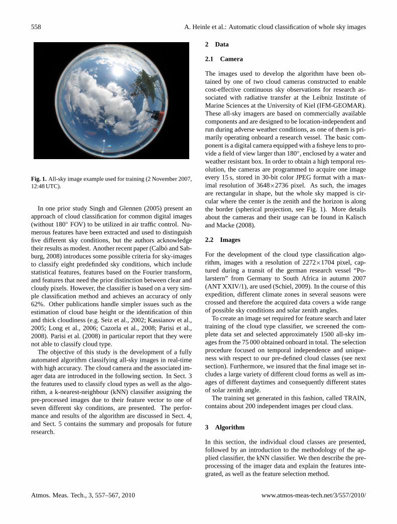
Fig. 1. All-sky image example used for training (02 November2007, 12:48 UTC).Fig. 1. All-sky image example used for training (2 November 2007,12:48 UTC).
In one prior studySingh and Glennen(2005) present anapproach of cloud classification for common digital images(without 180◦ FOV) to be utilized in air traffic control. Nu-merous features have been extracted and used to distinguishfive different sky conditions, but the authors acknowledgetheir results as modest. Another recent paper (Calbo and Sab-burg, 2008) introduces some possible criteria for sky-imagesto classify eight predefinded sky conditions, which includestatistical features, features based on the Fourier transform,and features that need the prior distinction between clear andcloudy pixels. However, the classifier is based on a very sim-ple classification method and achieves an accuracy of only62%. Other publications handle simpler issues such as theestimation of cloud base height or the identification of thinand thick cloudiness (e.g.Seiz et al., 2002; Kassianov et al.,2005; Long et al., 2006; Cazorla et al., 2008; Parisi et al.,2008). Parisi et al.(2008) in particular report that they werenot able to classify cloud type.
The objective of this study is the development of a fullyautomated algorithm classifying all-sky images in real-timewith high accuracy. The cloud camera and the associated im-ager data are introduced in the following section. In Sect. 3the features used to classify cloud types as well as the algo-rithm, a k-nearest-neighbour (kNN) classifier assigning thepre-processed images due to their feature vector to one ofseven different sky conditions, are presented. The perfor-mance and results of the algorithm are discussed in Sect. 4,and Sect. 5 contains the summary and proposals for futureresearch.
2 Data
2.1 Camera
The images used to develop the algorithm have been ob-tained by one of two cloud cameras constructed to enablecost-effective continuous sky observations for research as-sociated with radiative transfer at the Leibniz Institute ofMarine Sciences at the University of Kiel (IFM-GEOMAR).These all-sky imagers are based on commercially availablecomponents and are designed to be location-independent andrun during adverse weather conditions, as one of them is pri-marily operating onboard a research vessel. The basic com-ponent is a digital camera equipped with a fisheye lens to pro-vide a field of view larger than 180◦, enclosed by a water andweather resistant box. In order to obtain a high temporal res-olution, the cameras are programmed to acquire one imageevery 15 s, stored in 30-bit color JPEG format with a max-imal resolution of 3648×2736 pixel. As such, the imagesare rectangular in shape, but the whole sky mapped is cir-cular where the center is the zenith and the horizon is alongthe border (spherical projection, see Fig.1). More detailsabout the cameras and their usage can be found inKalischand Macke(2008).
2.2 Images
For the development of the cloud type classification algo-rithm, images with a resolution of 2272×1704 pixel, cap-tured during a transit of the german research vessel “Po-larstern” from Germany to South Africa in autumn 2007(ANT XXIV/1), are used (Schiel, 2009). In the course of thisexpedition, different climate zones in several seasons werecrossed and therefore the acquired data covers a wide rangeof possible sky conditions and solar zenith angles.
To create an image set required for feature search and latertraining of the cloud type classifier, we screened the com-plete data set and selected approximately 1500 all-sky im-ages from the 75 000 obtained onboard in total. The selectionprocedure focused on temporal independence and unique-ness with respect to our pre-defined cloud classes (see nextsection). Furthermore, we insured that the final image set in-cludes a large variety of different cloud forms as well as im-ages of different daytimes and consequently different statesof solar zenith angle.
The training set generated in this fashion, called TRAIN,contains about 200 independent images per cloud class.
3 Algorithm
In this section, the individual cloud classes are presented,followed by an introduction to the methodology of the ap-plied classifier, the kNN classifier. We then describe the pre-processing of the imager data and explain the features inte-grated, as well as the feature selection method.
Atmos. Meas. Tech., 3, 557–567, 2010 www.atmos-meas-tech.net/3/557/2010/
A. Heinle et al.: Automatic cloud classification of whole sky images 559
Table 1. Classes to be distinguished.
Label Cloud genera according to WMO Description
1 Cumulus Low, puffy clouds with clearly defined edges, white or light-grey2 Cirrus & Cirrostratus High, thin clouds, wisplike or sky covering, whitish3 Cirrocumulus & Altocumulus High patched clouds of small cloudlets, mosaic-like, white4 Clear sky No clouds and cloudiness below 10%5 Stratocumulus Low or mid-level, lumpy layer of clouds, broken to almost overcast, white or grey6 Stratus & Altostratus Low or mid-level layer of clouds, uniform, usually overcast, grey7 Cumulonimbus & Nimbostratus Dark, thick clouds, mostly overcast, grey
3.1 Cloud classes
In contrast to other publications handling automated cloudclassification, we used phenomenological classes to be sepa-rated according to the International Cloud Classification Sys-tem (ICCS) published inWMO (1987). Therein, ten generaare defined which represent the basis of our classification.Based on visual similarity we combined some genera (al-tostratus and stratus, cirrocumulus and altocumulus, cumu-lonimbus and nimbostratus) to avoid systematical misclassi-fications. Aditionally, we merged the genera cirrus and cir-rostratus due to lack of available data showing the latter, aswell as the difficulty in detecting very thin clouds, such assome kinds of cirrostratus. Besides, it must be noted that theclass of clear sky includes not only images without clouds,but also images with cloudiness below 10%.
Despite these generalizations, the resulting classes (see Ta-ble1) represent a suitable partitioning of possible sky condi-tions and are especially useful for radiation studies. In or-der to simplify the application of the cloud classes, each islabeled by an individual identification number (see also Ta-ble1).
3.2 Classifier
To classify the images described in Sect.2, the k-nearest-neighbour (kNN) method is chosen, which is part of the su-pervised, non-parametric classifiers (Duda and Hart, 2001).“Supervised” means that the separating classes are knownand a training sample is used to train the classifier. Non-parametric classifiers in general do not assume an a-prioriprobability distribution. Compared with other classifiers, thekNN method is very simple (and therefore associated withonly low computatitional costs) and simultaneously quitepowerful (Serpico et al., 1996; Vincent and Bengio, 2001;Duda and Hart, 2001). Even in the specific field of cloudtype recognition, some results for comparison with linearclassifiers and neural networks exist, underlining the highperformance of kNN classifiers (Singh and Glennen, 2005;Christodoulou et al., 2003).
kNN classifier.The assignment of an image to a specificclass using kNN classifiers is performed by majority vote.After pre-processing, several spectral and textural features
are extracted from an image. In the next step, the computedand normalized feature vectorx is compared with the knownfeature vectorsxi of each element in the training data bymeans of a distance measure, in our case the Manhattan Dis-tance
d(x,xi) :=
dim∑j=1
|xj −xij |. (1)
The class associated with the majority of thek closestmatches determines the unknown class. In the case that thismajority is not unique, the training date with the absolutesmallest distance to the unknown image specifies the targetclass. Therefore, the composition of the training sample anda meticulous selection of suitable images is of great impor-tance.
Complexity.The kNN classifier is often critizised for slowruntime performance and large memory requirements (inother words high time and space complexity, respectively).The time complexity of an algorithm is a measure of howmuch computation time is needed to run the algorithm andis thus dependent on the number of calculation steps. In thecase of image classification, this measure refers to the com-putational expense in classifying an unknown image. Usingthe kNN classifier, all distances between the feature vectorof this image and each of then members of the training sam-ple are required for the calculation. These distances dependon the dimensiond of the feature vector and we get a totalcomplexity ofO(nd) (heren = 1497 andd = 12).
Since kNN methods store a set of prototypes in memoryonce, the space complexity of such an algorithm isO(nd)as well.
3.3 Pre-processing
To obtain suitable features for separating the defined classes,it is necessary to eliminate some areas of the analysed rawimages, as they are rectangular in shape but the interestingpart, the mapped sky, is circular. Due to varied camera lo-cations, disruptive factors like ship superstructures or tower-ing edifices may also be mapped on the image and shouldbe excluded as well from further calculations. Additionally,
www.atmos-meas-tech.net/3/557/2010/ Atmos. Meas. Tech., 3, 557–567, 2010
560 A. Heinle et al.: Automatic cloud classification of whole sky images
A. Heinle et al.: Automatic cloud classification of whole sky images 9
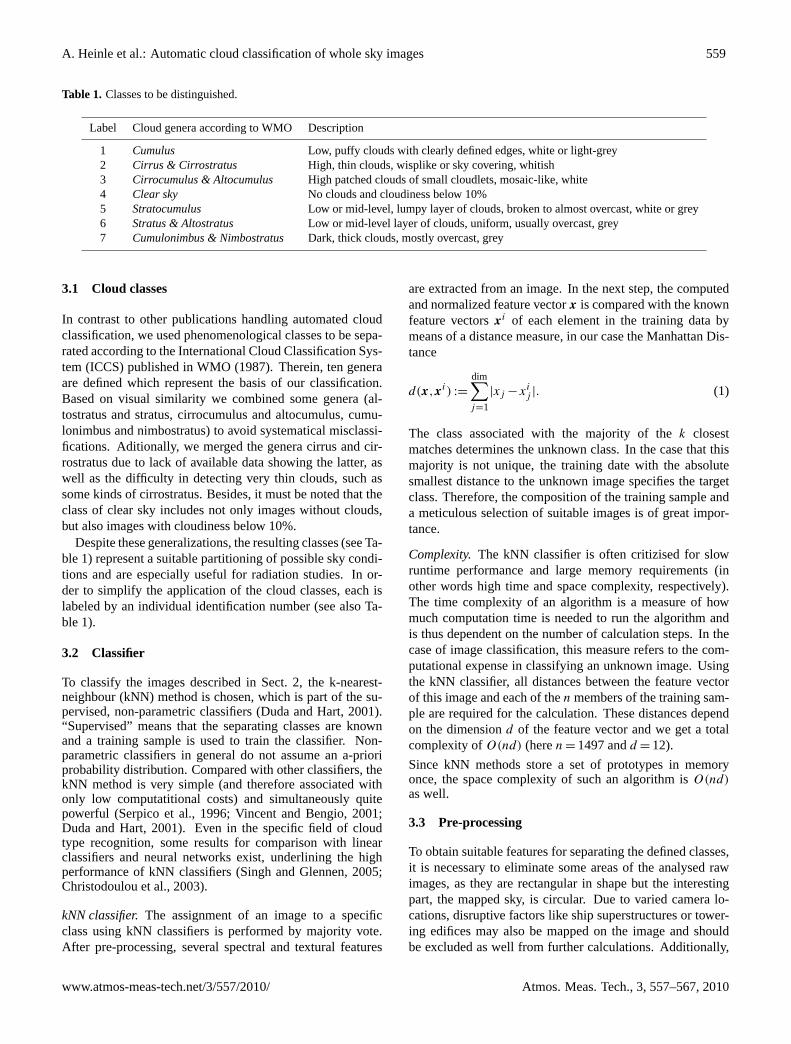
Fig. 2. Segmentation for optical thick clouds (top) and clear sky (bottom) using a treshold of R/B = 0.8 (middle) and a treshold ofR−B = 30 (right).
Fig. 3. Misclassification of clear sky caused by the “whitening effect” (left) and missclassification of stratus due to raindrops (right).
Fig. 2. Segmentation for optical thick clouds (top) and clear sky (bottom) using a treshold ofR/B = 0.8 (middle) and a treshold ofR−B = 30(right).
analyses showed that it is useful to segment the images intoclear and cloudy areas before calculating features.
Therefore, an image-mask, constructed by visually identi-fying image regions containing confounding information, isused first. The mask adapts the detected sections as well ascompletely white pixels (such as the ones displaying the sun)to the background by setting all corresponding pixel valuesto zero. Afterwards the remaining area is divided pixel bypixel into clear and cloudy regions, utilizing their red andblue pixel values.
In a clear atmosphere (without aerosols), more blue thanred light is scattered by gas molecules, which is why clearsky appears blue to our eyes. In contrast, clouds (contain-ing particles like aerosols, water droplets and/or ice crystals)scatter blue and red light to a similar extent, causing themto appear white or grey (Petty, 2006). Therefore, image re-gions with clear sky show relatively lower red pixel valuescompared to regions showing clouds, and the ratioR/B maybe used to differentiate these areas. A separating threshold,whose exact value depends on both the camera used and pre-vailing atmospheric conditions, has to be determined. Suit-able values are discussed in several papers handling cloudcover estimation (e.g.Pfister et al., 2003; Long et al., 2006).
However, during the testing phase we noticed problems indetecting thick clouds and classifying circumsolar pixels atthe same time. Therefore we modified the criterion and con-sidered the differenceR−B instead of the ratioR/B. Com-parisons showed that segmentation using such a differencethreshold still results in minor errors, but outperforms theratio method. For our application the valueR −B = 30 isoptimal (see Fig.2).
3.4 Features used
Out of numerous features tested (for example, features de-scribing edge or color, features considering the run-length ofprimitives, their quantity or frequency, or features describingthe texture of an image), we selected 12 features for appli-cation (see below). The choice of these features is based ontheir Fisher DistancesF x
ij , a selection criterion used in cloudclassification work relating to satellite imagery (Pankiewicz,1995). It is defined as
F xij :=
|µxi −µx
j |
σ xi +σ x
j
, (2)
Atmos. Meas. Tech., 3, 557–567, 2010 www.atmos-meas-tech.net/3/557/2010/
A. Heinle et al.: Automatic cloud classification of whole sky images 561
whereµxi and µx
j are the means of featurex with respectto classi andj , σ x
i andσ xj the corresponding standard de-
viations. The features best suited to separate the definedclasses are those which have the largest Fisher distancesF x
ij .It should be noted, however, that the feature set chosen inthis way has to guarantee the separation of all classes. Thatmeans that features with smaller Fisher distances have to beincluded in the final set as well, if they discriminate classeswhich are not separated by other features with higher dis-tances.
Most of the features are based on grey-scale images. Sincethe original data is provided in color, a partition into the threecomponents R, G and B has to be performed before the fea-tures can be calculated. A simple transformation providesthe grey-scale images, containing only the color informationof one channel (R, G or B).
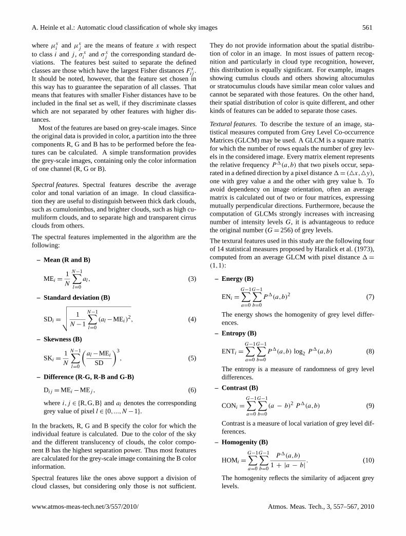
Spectral features.Spectral features describe the averagecolor and tonal variation of an image. In cloud classifica-tion they are useful to distinguish between thick dark clouds,such as cumulonimbus, and brighter clouds, such as high cu-muliform clouds, and to separate high and transparent cirrusclouds from others.
The spectral features implemented in the algorithm are thefollowing:
– Mean (R and B)
MEi =1
N
N−1∑l=0
al, (3)
– Standard deviation (B)
SDi =
√√√√ 1
N −1
N−1∑l=0
(al −MEi)2, (4)
– Skewness (B)
SKi =1
N
N−1∑l=0
(al −MEi
SD
)3
, (5)
– Difference (R-G, R-B and G-B)
Dij = MEi −MEj , (6)
wherei,j ∈ {R,G,B} andal denotes the correspondinggrey value of pixell ∈ {0,...,N −1}.
In the brackets, R, G and B specify the color for which theindividual feature is calculated. Due to the color of the skyand the different translucency of clouds, the color compo-nent B has the highest separation power. Thus most featuresare calculated for the grey-scale image containing the B colorinformation.
Spectral features like the ones above support a division ofcloud classes, but considering only those is not sufficient.
They do not provide information about the spatial distribu-tion of color in an image. In most issues of pattern recog-nition and particularly in cloud type recognition, however,this distribution is equally significant. For example, imagesshowing cumulus clouds and others showing altocumulusor stratocumulus clouds have similar mean color values andcannot be separated with those features. On the other hand,their spatial distribution of color is quite different, and otherkinds of features can be added to separate those cases.
Textural features.To describe the texture of an image, sta-tistical measures computed from Grey Level Co-occurrenceMatrices (GLCM) may be used. A GLCM is a square matrixfor which the number of rows equals the number of grey lev-els in the considered image. Every matrix element representsthe relative frequencyP 1(a,b) that two pixels occur, sepa-rated in a defined direction by a pixel distance1 = (4x,4y),one with grey value a and the other with grey value b. Toavoid dependency on image orientation, often an averagematrix is calculated out of two or four matrices, expressingmutually perpendicular directions. Furthermore, because thecomputation of GLCMs strongly increases with increasingnumber of intensity levelsG, it is advantageous to reducethe original number (G = 256) of grey levels.
The textural features used in this study are the following fourof 14 statistical measures proposed byHaralick et al.(1973),computed from an average GLCM with pixel distance1 =
(1,1):
– Energy (B)
ENi =
G−1∑a=0
G−1∑b=0
P 1(a,b)2 (7)
The energy shows the homogenity of grey level differ-ences.
– Entropy (B)
ENTi =
G−1∑a=0
G−1∑b=0
P 1(a,b) log2 P 1(a,b) (8)
The entropy is a measure of randomness of grey leveldifferences.
– Contrast (B)
CONi =
G−1∑a=0
G−1∑b=0
(a − b)2 P 1(a,b) (9)
Contrast is a measure of local variation of grey level dif-ferences.
– Homogenity (B)
HOMi =
G−1∑a=0
G−1∑b=0
P 1(a,b)
1 + |a − b|. (10)
The homogenity reflects the similarity of adjacent greylevels.
www.atmos-meas-tech.net/3/557/2010/ Atmos. Meas. Tech., 3, 557–567, 2010
562 A. Heinle et al.: Automatic cloud classification of whole sky images
Table 2. Confusion matrix ofCV for equally involved features in %.
True Classified as CV
class 1 2 3 4 5 6 7
1 93.73 1.57 4.31 0.39 0.00 0.00 0.002 0.72 97.13 1.07 1.07 0.00 0.00 0.003 2.49 1.93 95.30 0.00 0.28 0.00 0.004 0.00 1.20 0.00 98.80 0.00 0.00 0.005 0.00 0.00 0.00 0.00 96.43 3.57 0.006 0.00 0.00 0.94 0.00 0.00 96.23 2.837 0.00 0.00 1.84 0.00 1.38 0.00 96.77 96.13
Cloud cover.In addition to the features described above, wecomputed the cloud cover (CC):
– Cloud cover
CC:=Nbew
N, (11)
whereNbew denotes the number of cloudy pixels.
CC is a measure of the average cloudiness, and for examplestratiform clouds could be well distinguished from other skyconditions using this feature.
For each pre-classified image in the training sample TRAINwe computed the features presented and stored them withtheir assigned cloud class. Since the kNN classifer choosesthe target class of an unknown image based on its distancein the feature space to the training images and the featuresdiffer in their value ranges, we normalized the features to theinterval [0,100]. This ensures that all features are equallyweighted in the decision process.
4 Results and discussion
In this section we describe the methodology used to estimatethe performance of the created algorithm as well as to opti-mize the included parameters and the respective results arediscussed. Afterwards, an additional test sample of randomimages is presented to assess the performance of the algo-rithm in classifying more ambiguous images.
The algorithm was implemented in IDL and tested on anIntel Celeron 530 with 1.73 GHz and 512 MB RAM. For oneimage it took about 1.3 s to return the classification result.
4.1 Methodology of performance estimation
To estimate the performance of the selected features andthe created algorithm we applied the Leave-One-Out Cross-Validation (LOOCV). Cross validation methods in generalhave the advantage that they reuse the known training sam-ple to estimate the capability of an algorithm, neverthelessbeing unbiased, instead of needing an additional test sample
(Ripley, 2005). Therefore, they are often used for valida-tion or feature selection in the area of pattern recognition. Incloud type recognition the LOOCV has been applied by e.g.Tag et al.(2000) or Bankert and Wade(2007).
LOOCV. From the training sampleT , one single elementt isremoved and the algorithm is trained with the remaining data(T − t). Then the element excluded, which is independentfrom the data used for training, is classified. This is repeatedn times, wheren is the number of elements inT , such thateach element in the training sample is used for validation ex-actly once. The average number of correctly classified ele-ments
CV =|{t ∈ T |t is classified correctly}|
n(12)
is finally used as measure of performance.
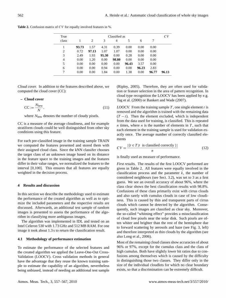
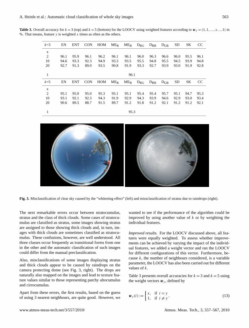
First results. The results of the first LOOCV performed aregiven in Table2. All features were equally involved in theclassification process and the parameterk, the number ofconsidered neighbours (see Sect.3.2), was set to 3 as a firstguess. We see an overall accuracy of about 96%, where theclass clear shows the best classification results with 98.8%.Confusions of these class primarily exist with cirrus cloudsand also rarely with cumulus clouds in case of low cloudi-ness. This is caused by thin and transparent parts of cirrusclouds which cannot be detected by the algorithm. Conse-quently, such images are classified as clear sky. Moreover,the so-called “whitning effect” provides a missclassificationof cloud free pixels near the solar disk. Such pixels are of-ten whiter and brighter than the rest of the hemisphere dueto forward scattering by aerosols and haze (see Fig.3, left)and therefore interpreted as thin clouds by the algorithm (seealsoLong et al., 2006).
Most of the remaining cloud classes show accuracies of about96% or 97%, except for the cumulus class and the class ofhigh cumulus. Both have slightly lower hit ratios due to con-fusions among themselves which is caused by the difficultyin distinguishing those two classes. They differ only in thesize of the individual cloudlets for which no clear boundaryexists, so that a discrimination can be extremely difficult.
Atmos. Meas. Tech., 3, 557–567, 2010 www.atmos-meas-tech.net/3/557/2010/
A. Heinle et al.: Automatic cloud classification of whole sky images 563
Table 3. Overall accuracy fork = 3 (top) andk = 5 (bottom) for the LOOCV using weighted features according towy = (1,1,....,x,..,1) in%. That means, featurey is weightedx times as often as the others.
k=3 EN ENT CON HOM MER MEB DRG DRB DGB SD SK CC
x2 96.1 95.9 96.1 96.2 96.1 96.1 96.0 96.3 96.6 96.0 95.5 96.110 94.6 93.3 92.3 94.9 93.3 93.5 95.5 94.8 95.5 94.5 93.9 94.820 92.7 91.3 89.0 93.5 90.8 91.9 93.3 92.7 93.9 93.0 91.9 92.8
1 96.1
k=5 EN ENT CON HOM MER MEB DRG DRB DGB SD SK CC
x2 95.1 95.0 95.0 95.3 95.1 95.1 95.4 95.4 95.7 95.1 94.7 95.310 93.1 92.1 92.3 94.3 91.9 92.9 94.3 93.9 94.6 92.9 93.0 93.420 90.6 89.5 88.7 91.5 89.7 91.2 91.8 91.2 92.1 91.2 91.2 92.1
1 95.3
A. Heinle et al.: Automatic cloud classification of whole sky images 9
Fig. 2. Segmentation for optical thick clouds (top) and clear sky (bottom) using a treshold of R/B = 0.8 (middle) and a treshold ofR−B = 30 (right).
Fig. 3. Misclassification of clear sky caused by the “whitening effect” (left) and missclassification of stratus due to raindrops (right).
A. Heinle et al.: Automatic cloud classification of whole sky images 9
Fig. 2. Segmentation for optical thick clouds (top) and clear sky (bottom) using a treshold of R/B = 0.8 (middle) and a treshold ofR−B = 30 (right).
Fig. 3. Misclassification of clear sky caused by the “whitening effect” (left) and missclassification of stratus due to raindrops (right).Fig. 3. Misclassification of clear sky caused by the “whitening effect” (left) and missclassification of stratus due to raindrops (right).
The next remarkable errors occur between stratocumulus,stratus and the class of thick clouds. Some cases of stratocu-mulus are classified as stratus, some images showing stratusare assigned to those showing thick clouds and, in turn, im-ages with thick clouds are sometimes classified as stratocu-mulus. These confusions, however, are well understood. Allthree classes occur frequently as transitional forms from onein the other and the automatic classification of such imagescould differ from the manual preclassification.
Also, misclassifications of some images displaying stratusand thick clouds appear to be caused by raindrops on thecamera protecting dome (see Fig.3, right). The drops arenaturally also mapped on the images and lead to texture fea-ture values similar to those representing patchy altocumulusand cirrocumulus.
Apart from these errors, the first results, based on the guessof using 3 nearest neighbours, are quite good. However, we
wanted to see if the performance of the algorithm could beimproved by using another value ofk or by weighting theindividual features.
Improved results.For the LOOCV discussed above, all fea-tures were equally weighted. To assess whether improve-ments can be achieved by varying the impact of the individ-ual features, we added a weight vector and ran the LOOCVfor different configurations of this vector. Furthermore, be-causek, the number of neighbours considered, is a variableparameter, the LOOCV has also been carried out for differentvalues ofk.
Table3 presents overall accuracies fork = 3 andk = 5 usingthe weight vectorswy , defined by
wy(i) :=
{x, if i = y
1, if i 6= y, (13)
www.atmos-meas-tech.net/3/557/2010/ Atmos. Meas. Tech., 3, 557–567, 2010
564 A. Heinle et al.: Automatic cloud classification of whole sky images
Table 4. Confusion matrix ofCV for optimal weighted features in %.
True Classified as CV
class 1 2 3 4 5 6 7
1 96.47 1.18 1.96 0.39 0.00 0.00 0.002 0.72 98.57 0.36 0.36 0.00 0.00 0.003 1.93 1.66 96.41 0.00 0.00 0.00 0.004 0.00 1.20 0.00 98.80 0.00 0.00 0.005 0.00 0.00 0.00 0.00 95.54 3.57 0.896 0.00 0.00 0.00 0.00 1.89 94.34 3.777 0.00 0.00 1.84 0.00 0.46 0.00 97.70 97.06
10 A. Heinle et al.: Automatic cloud classification of whole sky images
Fig. 4. Image showing cirrus and cumulus clouds (04 November 2007, 09:39 UTC) (left), image showing clear sky during a dust event (08November 2007, 13:40 UTC) (right).
Table 1. Classes to be distinguished.
Label Cloud genera according to WMO Description
1 Cumulus Low, puffy clouds with clearly defined edges, white or light-grey2 Cirrus & Cirrostratus Cirrus clouds, wisplike or sky covering, whitish, thin3 Cirrocumulus & Altocumulus High patched clouds of small cloudlets, mosaic-like, white4 Clear sky No clouds and cloudiness below 10 %5 Stratocumulus Low or mid-level, lumpy layer of clouds, broken to almost overcast, white or grey6 Stratus & Altostratus Low or mid-level layer of clouds, uniform, grey, usually overcast7 Cumulonimbus & Nimbostratus Dark, thick clouds, grey, mostly overcast
Table 2. Confusion matrix of CV for equally involved features in %.
True Classified as CVclass 1 2 3 4 5 6 7
1 93.73 1.57 4.31 0.39 0.00 0.00 0.002 0.72 97.13 1.07 1.07 0.00 0.00 0.003 2.49 1.93 95.30 0.00 0.28 0.00 0.004 0.00 1.20 0.00 98.80 0.00 0.00 0.005 0.00 0.00 0.00 0.00 96.43 3.57 0.006 0.00 0.00 0.94 0.00 0.00 96.23 2.837 0.00 0.00 1.84 0.00 1.38 0.00 96.77 96.13
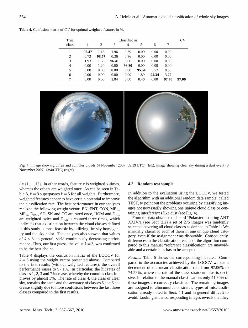
Fig. 4. Image showing cirrus and cumulus clouds (4 November 2007, 09:39 UTC) (left), image showing clear sky during a dust event (8November 2007, 13:40 UTC) (right).
i ∈ {1,...,12}. In other words, feature y is weighted x-times,whereas the others are weighted once. As can be seen in Ta-ble 3, k = 3 superpassesk = 5 for all weights. Furthermore,weighted features appear to have certain potential to improvethe classification rate. The best performance in our analysesrealized the following weight vector: EN, ENT, CON, MER,MEB, DRG, SD, SK and CC are rated once, HOM and DRBare weighted twice and DGB is counted three times, whichindicates that a distinction between the cloud classes definedin this study is most feasible by utilizing the sky homogen-ity and the sky color. The analyses also showed that valuesof k > 3, in general, yield continuously decreasing perfor-mance. Thus, our first guess, the valuek = 3, was confirmedto be the best choice.
Table 4 displays the confusion matrix of the LOOCV fork = 3 using the weight vector presented above. Comparedto the first results (without weighted features), the overallperformance raises to 97.1%. In particular, the hit rates ofclasses 1, 2, 3 and 7 increase, whereby the cumulus class im-proves by almost 3%. The rate of class 4, the class of clearsky, remains the same and the accuracy of classes 5 and 6 de-crease slightly due to more confusions between the last threeclasses compared to the first results.
4.2 Random test sample
In addition to the evaluation using the LOOCV, we testedthe algorithm with an additional random data sample, calledTEST, to point out the problems occuring by classifying im-ages not necessarily showing one unique cloud class or con-taining interferences like dust (see Fig.4).
From the data obtained on board “Polarstern” during ANTXXIV/1 (see Sect.2.2) a set of 275 images was randomlyselected, covering all cloud classes as defined in Table1. Wemanually classified each of them in one unique cloud cate-gory, even if the assignment was disputable. Consequently,differences in the classification results of the algorithm com-pared to this manual “reference classification” are unavoid-able and a certain bias has to be accepted.
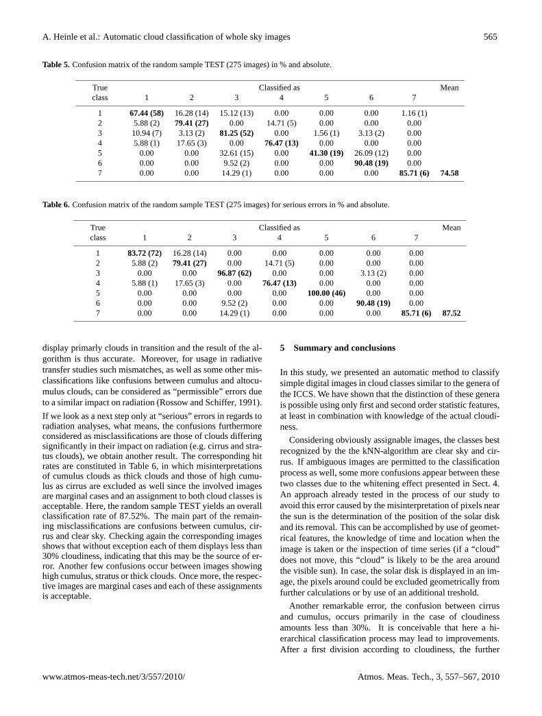
Results.Table 5 shows the corresponding hit rates. Com-pared to the accuracies achieved by the LOOCV we see adecrement of the mean classification rate from 97.06% to74.58%, where the rate of the class stratocumulus is deci-sive. In relation to the manual classification, only 41.30% ofthese images are correctly classified. The remaining imagesare assigned to altocumulus or stratus, types of misclassifi-cation already noted in Sect.4.1 and in general difficult toavoid. Looking at the corresponding images reveals that they
Atmos. Meas. Tech., 3, 557–567, 2010 www.atmos-meas-tech.net/3/557/2010/
A. Heinle et al.: Automatic cloud classification of whole sky images 565
Table 5. Confusion matrix of the random sample TEST (275 images) in % and absolute.
True Classified as Meanclass 1 2 3 4 5 6 7
1 67.44 (58) 16.28 (14) 15.12 (13) 0.00 0.00 0.00 1.16 (1)2 5.88 (2) 79.41 (27) 0.00 14.71 (5) 0.00 0.00 0.003 10.94 (7) 3.13 (2) 81.25 (52) 0.00 1.56 (1) 3.13 (2) 0.004 5.88 (1) 17.65 (3) 0.00 76.47 (13) 0.00 0.00 0.005 0.00 0.00 32.61 (15) 0.00 41.30 (19) 26.09 (12) 0.006 0.00 0.00 9.52 (2) 0.00 0.00 90.48 (19) 0.007 0.00 0.00 14.29 (1) 0.00 0.00 0.00 85.71 (6) 74.58
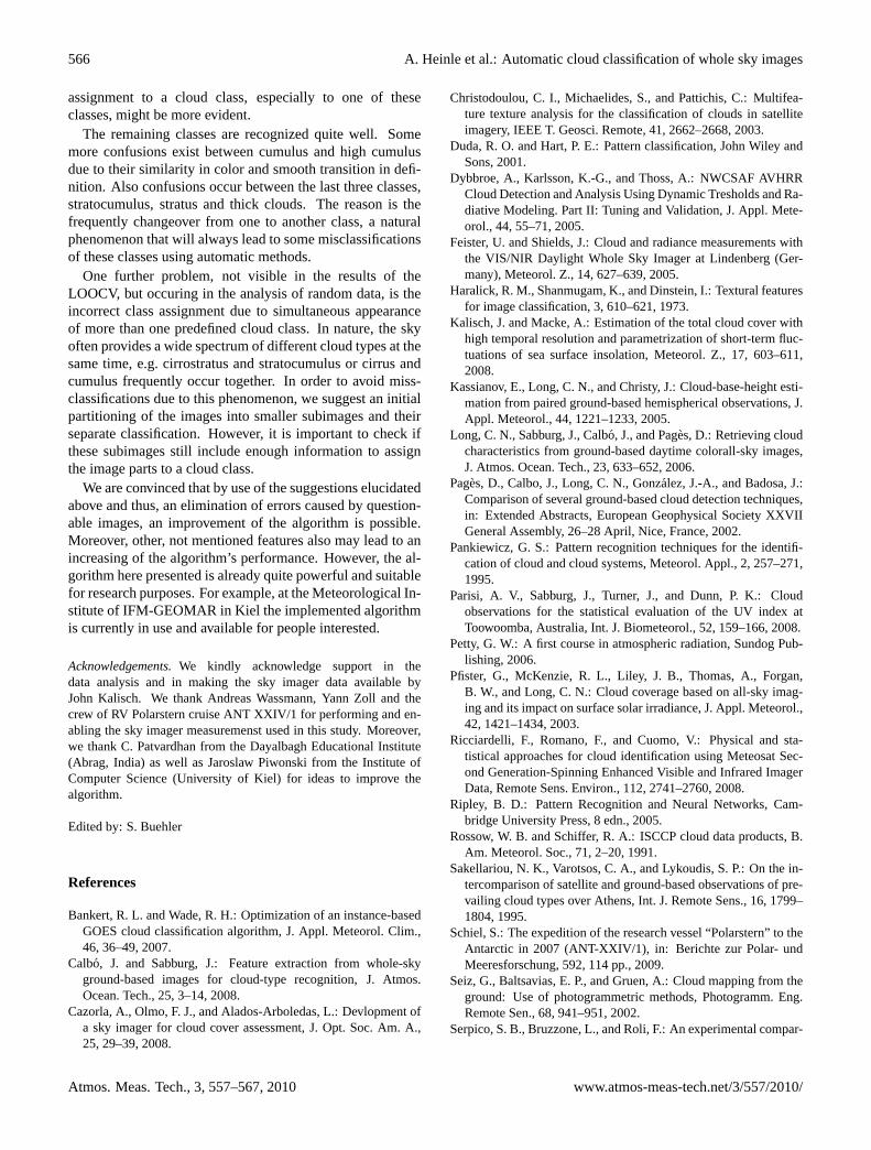
Table 6. Confusion matrix of the random sample TEST (275 images) for serious errors in % and absolute.
True Classified as Meanclass 1 2 3 4 5 6 7
1 83.72 (72) 16.28 (14) 0.00 0.00 0.00 0.00 0.002 5.88 (2) 79.41 (27) 0.00 14.71 (5) 0.00 0.00 0.003 0.00 0.00 96.87 (62) 0.00 0.00 3.13 (2) 0.004 5.88 (1) 17.65 (3) 0.00 76.47 (13) 0.00 0.00 0.005 0.00 0.00 0.00 0.00 100.00 (46) 0.00 0.006 0.00 0.00 9.52 (2) 0.00 0.00 90.48 (19) 0.007 0.00 0.00 14.29 (1) 0.00 0.00 0.00 85.71 (6) 87.52
display primarly clouds in transition and the result of the al-gorithm is thus accurate. Moreover, for usage in radiativetransfer studies such mismatches, as well as some other mis-classifications like confusions between cumulus and altocu-mulus clouds, can be considered as “permissible” errors dueto a similar impact on radiation (Rossow and Schiffer, 1991).
If we look as a next step only at “serious” errors in regards toradiation analyses, what means, the confusions furthermoreconsidered as misclassifications are those of clouds differingsignificantly in their impact on radiation (e.g. cirrus and stra-tus clouds), we obtain another result. The corresponding hitrates are constituted in Table6, in which misinterpretationsof cumulus clouds as thick clouds and those of high cumu-lus as cirrus are excluded as well since the involved imagesare marginal cases and an assignment to both cloud classes isacceptable. Here, the random sample TEST yields an overallclassification rate of 87.52%. The main part of the remain-ing misclassifications are confusions between cumulus, cir-rus and clear sky. Checking again the corresponding imagesshows that without exception each of them displays less than30% cloudiness, indicating that this may be the source of er-ror. Another few confusions occur between images showinghigh cumulus, stratus or thick clouds. Once more, the respec-tive images are marginal cases and each of these assignmentsis acceptable.
5 Summary and conclusions
In this study, we presented an automatic method to classifysimple digital images in cloud classes similar to the genera ofthe ICCS. We have shown that the distinction of these generais possible using only first and second order statistic features,at least in combination with knowledge of the actual cloudi-ness.
Considering obviously assignable images, the classes bestrecognized by the the kNN-algorithm are clear sky and cir-rus. If ambiguous images are permitted to the classificationprocess as well, some more confusions appear between thesetwo classes due to the whitening effect presented in Sect.4.An approach already tested in the process of our study toavoid this error caused by the misinterpretation of pixels nearthe sun is the determination of the position of the solar diskand its removal. This can be accomplished by use of geomet-rical features, the knowledge of time and location when theimage is taken or the inspection of time series (if a “cloud”does not move, this “cloud” is likely to be the area aroundthe visible sun). In case, the solar disk is displayed in an im-age, the pixels around could be excluded geometrically fromfurther calculations or by use of an additional treshold.
Another remarkable error, the confusion between cirrusand cumulus, occurs primarily in the case of cloudinessamounts less than 30%. It is conceivable that here a hi-erarchical classification process may lead to improvements.After a first division according to cloudiness, the further
www.atmos-meas-tech.net/3/557/2010/ Atmos. Meas. Tech., 3, 557–567, 2010
566 A. Heinle et al.: Automatic cloud classification of whole sky images
assignment to a cloud class, especially to one of theseclasses, might be more evident.
The remaining classes are recognized quite well. Somemore confusions exist between cumulus and high cumulusdue to their similarity in color and smooth transition in defi-nition. Also confusions occur between the last three classes,stratocumulus, stratus and thick clouds. The reason is thefrequently changeover from one to another class, a naturalphenomenon that will always lead to some misclassificationsof these classes using automatic methods.
One further problem, not visible in the results of theLOOCV, but occuring in the analysis of random data, is theincorrect class assignment due to simultaneous appearanceof more than one predefined cloud class. In nature, the skyoften provides a wide spectrum of different cloud types at thesame time, e.g. cirrostratus and stratocumulus or cirrus andcumulus frequently occur together. In order to avoid miss-classifications due to this phenomenon, we suggest an initialpartitioning of the images into smaller subimages and theirseparate classification. However, it is important to check ifthese subimages still include enough information to assignthe image parts to a cloud class.
We are convinced that by use of the suggestions elucidatedabove and thus, an elimination of errors caused by question-able images, an improvement of the algorithm is possible.Moreover, other, not mentioned features also may lead to anincreasing of the algorithm’s performance. However, the al-gorithm here presented is already quite powerful and suitablefor research purposes. For example, at the Meteorological In-stitute of IFM-GEOMAR in Kiel the implemented algorithmis currently in use and available for people interested.
Acknowledgements.We kindly acknowledge support in thedata analysis and in making the sky imager data available byJohn Kalisch. We thank Andreas Wassmann, Yann Zoll and thecrew of RV Polarstern cruise ANT XXIV/1 for performing and en-abling the sky imager measuremenst used in this study. Moreover,we thank C. Patvardhan from the Dayalbagh Educational Institute(Abrag, India) as well as Jaroslaw Piwonski from the Institute ofComputer Science (University of Kiel) for ideas to improve thealgorithm.
Edited by: S. Buehler
References
Bankert, R. L. and Wade, R. H.: Optimization of an instance-basedGOES cloud classification algorithm, J. Appl. Meteorol. Clim.,46, 36–49, 2007.
Calbo, J. and Sabburg, J.: Feature extraction from whole-skyground-based images for cloud-type recognition, J. Atmos.Ocean. Tech., 25, 3–14, 2008.
Cazorla, A., Olmo, F. J., and Alados-Arboledas, L.: Devlopment ofa sky imager for cloud cover assessment, J. Opt. Soc. Am. A.,25, 29–39, 2008.
Christodoulou, C. I., Michaelides, S., and Pattichis, C.: Multifea-ture texture analysis for the classification of clouds in satelliteimagery, IEEE T. Geosci. Remote, 41, 2662–2668, 2003.
Duda, R. O. and Hart, P. E.: Pattern classification, John Wiley andSons, 2001.
Dybbroe, A., Karlsson, K.-G., and Thoss, A.: NWCSAF AVHRRCloud Detection and Analysis Using Dynamic Tresholds and Ra-diative Modeling. Part II: Tuning and Validation, J. Appl. Mete-orol., 44, 55–71, 2005.
Feister, U. and Shields, J.: Cloud and radiance measurements withthe VIS/NIR Daylight Whole Sky Imager at Lindenberg (Ger-many), Meteorol. Z., 14, 627–639, 2005.
Haralick, R. M., Shanmugam, K., and Dinstein, I.: Textural featuresfor image classification, 3, 610–621, 1973.
Kalisch, J. and Macke, A.: Estimation of the total cloud cover withhigh temporal resolution and parametrization of short-term fluc-tuations of sea surface insolation, Meteorol. Z., 17, 603–611,2008.
Kassianov, E., Long, C. N., and Christy, J.: Cloud-base-height esti-mation from paired ground-based hemispherical observations, J.Appl. Meteorol., 44, 1221–1233, 2005.
Long, C. N., Sabburg, J., Calbo, J., and Pages, D.: Retrieving cloudcharacteristics from ground-based daytime colorall-sky images,J. Atmos. Ocean. Tech., 23, 633–652, 2006.
Pages, D., Calbo, J., Long, C. N., Gonzalez, J.-A., and Badosa, J.:Comparison of several ground-based cloud detection techniques,in: Extended Abstracts, European Geophysical Society XXVIIGeneral Assembly, 26–28 April, Nice, France, 2002.
Pankiewicz, G. S.: Pattern recognition techniques for the identifi-cation of cloud and cloud systems, Meteorol. Appl., 2, 257–271,1995.
Parisi, A. V., Sabburg, J., Turner, J., and Dunn, P. K.: Cloudobservations for the statistical evaluation of the UV index atToowoomba, Australia, Int. J. Biometeorol., 52, 159–166, 2008.
Petty, G. W.: A first course in atmospheric radiation, Sundog Pub-lishing, 2006.
Pfister, G., McKenzie, R. L., Liley, J. B., Thomas, A., Forgan,B. W., and Long, C. N.: Cloud coverage based on all-sky imag-ing and its impact on surface solar irradiance, J. Appl. Meteorol.,42, 1421–1434, 2003.
Ricciardelli, F., Romano, F., and Cuomo, V.: Physical and sta-tistical approaches for cloud identification using Meteosat Sec-ond Generation-Spinning Enhanced Visible and Infrared ImagerData, Remote Sens. Environ., 112, 2741–2760, 2008.
Ripley, B. D.: Pattern Recognition and Neural Networks, Cam-bridge University Press, 8 edn., 2005.
Rossow, W. B. and Schiffer, R. A.: ISCCP cloud data products, B.Am. Meteorol. Soc., 71, 2–20, 1991.
Sakellariou, N. K., Varotsos, C. A., and Lykoudis, S. P.: On the in-tercomparison of satellite and ground-based observations of pre-vailing cloud types over Athens, Int. J. Remote Sens., 16, 1799–1804, 1995.
Schiel, S.: The expedition of the research vessel “Polarstern” to theAntarctic in 2007 (ANT-XXIV/1), in: Berichte zur Polar- undMeeresforschung, 592, 114 pp., 2009.
Seiz, G., Baltsavias, E. P., and Gruen, A.: Cloud mapping from theground: Use of photogrammetric methods, Photogramm. Eng.Remote Sen., 68, 941–951, 2002.
Serpico, S. B., Bruzzone, L., and Roli, F.: An experimental compar-
Atmos. Meas. Tech., 3, 557–567, 2010 www.atmos-meas-tech.net/3/557/2010/
A. Heinle et al.: Automatic cloud classification of whole sky images 567
ison of neural and statistical non-parametric algorithms for su-pervised classification of remote-sensing images, Pattern Recog-nit. Lett., 17, 1331–1341, 1996.
Shields, J. E., Johnson, R. W., Karr, M. E., and Wertz, J. L.: Au-tomated day/night whole sky imagers for field assessment ofcloud cover distributions and radiance distributions, in: Proc.10th Symp. on Meteorological Observations and Instrumenta-tion, 11–16 January, Boston, MA, 1998.
Shields, J. E., Johnson, R. W., Karr, M. E., Burden, A. R., andBaker, J. G.: Daylight visible/NIR whole sky imagers for cloudand radiance monitoring in support of UV research programs, in:Proc. SPIE, vol. 5156, pp. 155–166, 2003.
Singh, M. and Glennen, M.: Automated ground-based cloud recog-nition, Pattern Anal. Appl., 8, 258–271, 2005.
Solomon, S., Qin, D., Manning, M., Chen, Z., Marquis, M., Averyt,K. B., Tignor, M., and Miller, H. L.: Climate Change 2007: ThePhysical Science Basis – Contribution of Working group I to theFourth Assessment Report of the IPCC, Cambridge UniversityPress, 2007.
Souza-Echer, M. P., Pereira, E. B., Bins, L. S., and Andrade, M.A. R.: A Simple Method for the Assessment of the Cloud CoverState in High-Latitude Regions by a Ground-Based Digital Cam-era, J. Atmos. Oceanic Technol., 23, 437–447, 2006.
Tag, P. M., Bankert, R. L., and Brody, L. R.: An AVHRR multiplecloud-type classification package, J. Appl. Meteorol., 39, 125–134, 2000.
Vincent, P. and Bengio, Y.: K-Local Hyperplane and Convex Dis-tance Nearest Neighbor Algorithms, Tech. rep., Dept. IRO, Uni-versite de Montreal, 2001.
WMO: International Cloud Atlas, Vol. 2, Am. Meteorol. Soc., 1987.
www.atmos-meas-tech.net/3/557/2010/ Atmos. Meas. Tech., 3, 557–567, 2010