Abstract—This paper describes the techniques to morph

between the two portions of sound originated from a common source, broken because of by some reason. We make use of morphing technique to join the sound where the pitch of the sound slowly changes from one broken part to another broken part by slowly changing the pitch information also covering the unvoiced region of the music. Spectral shapes are encoded on the multidimensional space while pitch on orthogonal axes of it. After matching components of the sound, a morph smoothly interpolates the amplitudes to describe a new sound in the same perceptual space. Finally, by inverting the representation, sound is produced. According to the literature survey, this is the first paper which explains the step by step evolution of one sound resulting into other sound across all states of intermediate steps along with the step by step runtime analysis. This will help researchers in future to improve the morphing methodology by looking carefully into the intermediate steps which decides the overall results. Here, we key out representations for morphing, techniques for matching, and interpolation algorithms and morphing each sound component. Spectral images of complete morph spectrogram are shown in the end.

Index Terms—Audio morphing, MFCC, dynamic time warping, interpolation.

I. INTRODUCTION There is high potential for audio morphing in sound

industry. The important applications of audio morphing include in speech recognition, speech synthesis, music synthesis, and other applications where large corpus database is recorded. Morphing is extensively used where interpolation is necessary between the exemplars of corpus database to produce the new one.

This paper describes techniques to automatically morph from one sound to another. Morphing in video is a process where the range of images is generated which are smoothly moved from one image to another. If all the images in-between smoothly change their shape and texture until it turns from one object to another is called as good morph. The same process performed in audio processing is termed as audio morph. A sound that is perceived as one object should change into another sound smoothly with variations in the

Manuscript received February 2, 2012; revised April 23, 2012. N S. Kumar, A. Singh, A. Reddy are with the Electrical Department of

National Institute of Technology, Warangal, India. (e-mail: amarjotsingh@ieee.org).

K S. Sruthi, is with the Electronics and Communication Department of National Institute of Technology, Warangal, India

parameters while maintaining the shared properties of starting and ending sounds.

Block diagram of morphing process is shown in fig 1. Audio morphing is accomplished by multi-dimensional representation of sound which can be warped or modified to produce a desired result. After matching components of the sound, a new morphed sound will describe the smooth interpolation of sound amplitudes in the same perceptual space. Finally, by inverting the representation, morphed sound is produced. The body of this paper describes representations for morphing, techniques for matching, and interpolation algorithms and morphing each sound component. Images of complete morph spectrogram are shown in the end.

II. PREVIOUS WORK Magnitude spectrogram techniques are described in this

paper. Far from complicating the problem, morphing can be done easily by spectrogram representation as we no longer have to track the sinusoids and their phase [1].

The sound having same magnitude spectrogram can be obtained by the inversion of spectrogram described in work elsewhere [2], without worrying about the phase information. Magnitude spectrogram representation of sound allows us to make dramatic changes to them without worrying about the phase. Recovery of phase can be done later during the spectrogram inversion process.

Automatic morphing techniques are described in this paper to morph from one sound to another. It is no longer easy to see the best matches as we make use of rich, multidimensional representation to describe sound. A method similar to auto-correspondence methods, as described for video [3], is used in this paper. Voice transformations [4] change the statistical properties of one speaker’s utterances to another voice. Therefore, if /i/ is spoken, the formant frequencies are changed every time to match the target speaker formants. This work, on the other hand, generates new sounds that are in between two exemplars.

III. IMPORTANCE OF TIME IN MORPHING Time is a special component of sound as sound cannot

exist without time. Audio morphing is simplified by this concept as sounds that happen at the same time are perceived together. Thus, the simultaneous components of sound should be kept aligned throughout the morph in audio morphing. This implies that, unlike in the image morphing, time is the important dimension which can be considered

Automatic Audio Morphing on Detached Sound Waveforms

N Sumanth Kumar, Amarjot Singh, Arundathy Reddy, and K Sai Sruthi

293

International Journal of Computer and Electrical Engineering, Vol. 4, No. 3, June 2012

independent of other dimensions. The morphs described here take the time as separate dimension from the other dimensions of the auditory signal for processing of speech. The ability to separate the time property simplifies all the aspects of audio morphing.

Fig. 1. Above are the three stages in morphing of sound namely

representation, matching and interpolation. The same procedure is applied to sound 2.

Time complicates other aspects of audio morphing. Most

importantly, audio morphing can be done in three different kinds. The simple case being that the two sounds are stationary and can be described as points in high-dimensional space which include spectral shape, pitch, rhythm and any other perceptually relevant (and quantifiable) auditory dimensions. We proceed to morph the two sounds by tracing a path between the two points in an appropriately warped space. This is directly analogous to the image morphing case. In the simplest form, a steady vowel morphs into a single note from an oboe.

The second approach for morphing is between moving objects. The morph starts with first sound characteristics and slowly changes to have the characteristics of second one. This is pretty similar to morphing between videos of two different objects.

Finally, a unique kind of audio morph is generated by smoothly changing a repetitive sequence of sounds. The word www in small sequential steps changes to zzz while in the middle of the sequence, the word sounds like something in between www and zzz. These results are in cyclo stationary morph as we play the sound repetitively to affect the morph. It is stationary since each sound instance is a completely stationary (no change) example of the range of in between sounds.

IV. DEPICTING THE SOUND IN VARIOUS FORMS Humans can very easily identify retinotopic image in a

video as it is natural and easy to change. In case of audio, we do not have any obvious choice like images to represent the sound. One disadvantage of conventional spectrograms is its inability to produce convincing morphs.

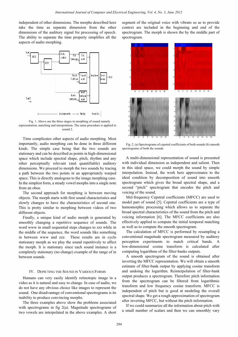
The three examples above show the problems associated with spectrograms in fig 2(a). Magnitude spectrograms of two vowels are interpolated in the above examples. A short

segment of the original voice with vibrato so as to provide context are included in the beginning and end of the spectrogram. The morph is shown the by the middle part of spectrogram.

Fig. 2. (a) Spectrograms of cepstral coefficients of both sounds (b) smooth

spectrograms of both the sounds A multi-dimensional representation of sound is presented

with individual dimension as independent and salient. Then in this ideal space, we could morph the sound by simple interpolation. Instead, the work here approximates to the ideal condition by decomposition of sound into smooth spectrogram which gives the broad spectral shape, and a second “pitch” spectrogram that encodes the pitch and voicing of the sound.

Mel-frequency Cepstral coefficients (MFCC) are used to model part of sound [5]. Cepstral coefficients are a type of hamomorphic processing which allows us to separate the broad spectral characteristics of the sound from the pitch and voicing information [6]. The MFCC coefficients are also effectively applied to compute the initial temporal matching as well as to compute the smooth spectrogram.

The calculation of MFCC is performed by resampling a conventional magnitude spectrogram measured by auditory perception experiments to match critical bands. A low-dimensional cosine transform is calculated after computing logarithms of the filter-banks outputs.

A smooth spectrogram of the sound is obtained after inverting the MFCC representation. We will obtain a smooth estimate of filter-bank output by applying cosine transform and undoing the logarithm. Reinterpolation of filter-bank output produces a spectrogram. Therefore pitch information from the spectrogram can be filtered from logarithmic transform and low frequency cosine transform. MFCC is independent of pitch but is good at modeling the overall spectral shape. We get a rough approximation of spectrogram after inverting MFCC, but without the pitch information.

If we could summarize all the information about pitch with a small number of scalars and then we can smoothly vary

294

International Journal of Computer and Electrical Engineering, Vol. 4, No. 3, June 2012

these numbers to get intermediate excitations very easily. But, this type of summarization as seen in speech compression systems is not sufficient. In the excitation, simple LPC systems suffer from objectionable inaccuracies. The summary of possible residues is needed in large codebook so as to provide acceptable reconstructions.

We make use of spectrogram of the residue to code the pitch and voicing in the acoustic signal of an audio morph. The total information in the signal is encoded by a conventional short-time spectrogram ( , )S tω while the overall spectral shape is defined by smooth spectrogram

( , )SS tω . We obtain “pitch” or residual spectrogram ( , )PS tω by dividing the short time spectrogram S by the

smooth spectrogram SS . The pitch spectrogram describes the pitch and voicing

information of the sound. The basis of our morphing techniques can be formed by smooth and pitch spectrograms. Thus, original spectrogram can be recovered by multiplying the pitch and smooth spectrograms together.

Fig. 3. Pitch spectrogram of both the sounds

V. MATCHING USING DTW The necessity of matching is to know which features of the

first sound correspond to any particular feature of the second. The feature is moved slowly from the position it is in first sound to its position in second so as to affect the morph. Number of ways are available to perform matching, but in audio morphing, Dynamic time warping and harmonic alignment are used.

The best temporal match is obtained by Dynamic Time Warping (DTW) between the two sounds. We want features that are common to both sounds to remain relatively fixed in time in the morph over its course. In modern speech recognition systems, MMCC is often used as a distance metric. For the later spectral stages to have less work, we make use of DTW which helps in calculating the best match between the two sounds.

By using different matching functions, audio morphs with different properties are created. Melody is important when morphing between two versions of the same song. With the distance metric based on the dominant pitch, temporal matching is performed. We consider the underlying rhythm for other music (i.e. rap).

Pitch and voicing information is represented as a spectrogram in this work. Series of peaks that are visible in the spectrogram shows the pitch information present in the sound. Pitch in the spectrogram is proportional to spacing between the peaks. The peaks disappear when the sound is unvoiced and spectrum of pitch become flat.

We need to match the pitch, if present so as to smoothly morph the pitch spectrogram, and then cross-fade the amplitude at each frequency. Sometimes, there is absence of pitch and sometimes, it is difficult to find it. At times, we have to deal when there is pitch in one sound and the other doesn’t. We want to match the pitch when it is available, else we cross-fade the noise.

The estimation of pitch is done for the entire utterance to solve this problem. Pitch is calculated by making use of conventional pitch scheme and dynamic programming. It is difficult for us to know the best pitch without further information since the basic pitch algorithm (autocorrelation of peak enhanced waveform) produces many possible pitch peaks

Fig. 4. (a) . Spectrograms obtained from DTW on cepstral coefficients (b)

spectrograms obtained from DTW on pitch spectrograms A novel algorithm was proposed by Secrest and

Doddington [7] using dynamic programming which can be effectively used to estimate the pitch changing smoothly over time which fits the available data (the peaks in the pitch spectrogram). By using this, pitch estimate for the entire sound is calculated whether it is actually voiced or not.

Complete pitch estimate from both the sounds are used to perform the match. Matching of the pitch between two sounds is very important and matching of the inharmonic residual is not much of importance. Frequency axis of pitch spectrogram is compressed or stretched to make sure that pitch peaks agree before crossfading the two spectrograms. The unvoiced components of the sound will move in frequency depending on the change in pitch. Splitting the harmonics which generate pitch is more important than the unvoiced component of speech.

It is less critical to match the features of the smooth spectrogram. Proper domain to match the features is investigated by the researchers to perform interpolation for voice coding [8]. Spectral shapes can be cross faded by interpolating the spectral peak locations by cross-fading line spectral pairs (LSP).

295

International Journal of Computer and Electrical Engineering, Vol. 4, No. 3, June 2012

VI. MORPHING IN SINGLE DIMENSION There is some kind of interpolation step which is used to

produce morph. It is easier to morph the scalar quantities because it reduces to simple cross-fade. In the sound description, loudness being one of the component, then the loudness in morph changes smoothly from the magnitude of first sound to the second.

Fig. 5. (a) Spectrograms obtained from DTW on pitch spectrograms (b) one-dimensional morphing did by warping along matching lines shown as

dashed lines for cross-fading the signals.

Acoustic information being not scalar always is also a cause for the problem in temporal alignment and spectral warping. Similar problem is shared by temporal alignment and spectral warping. How do we smoothly morph the curves if dense match is given between two one-dimensional curves?

1( )d t and 2 ( )d t is the data which we are trying to morph. The main aim is to find the function d such that the new curve ( , )d h t is between the curves 1d and 2d . Matching lines do not cross because the match functions are monotonic. So there is only one line establishing the match for each point ( , )h t . The problem is further simplified to find the times

1t and 2t by which data at ( , )h t is generated by interpolation. The time 1t for the path locations for all (sampled) values

is calculated and tracked to the path closest to the desired sample ( , )h t . The lines at 1t and 2t as shown in fig 5(b), intersect with the morphing line h at

12 1 1

2 1

( )t t

t h t t tt t

λ−= ⇒ = − +

− (1)

The new data at ( , )h t for 1t and 2t is generated by cross-fading the warped signals

1 1 2 2( , ) (1 ) ( ) ( )d t h d t hd tλ = − + (2)

The mappings from 1d to 2d are called paths. Path l warps 2d to look like 1d . Thus l is the mapping that generates the shortest difference between 2 ( ( ))d l t and 1( )d t . The above can be used to simplify the equation (ii) so that the intermediate t is given by

1 1 1( ( ) )t h l t t t= − + (3)

To calculate 2t , we use path map, but the better results are obtained when the procedure is repeated in other direction. On the same 2t , more than one might map along the axis due the quantization. We will not get an exact copy of 2d when

1h = , but some point will be little bit away from their place. The procedure used to find the best 1t is repeated to find best

2d for the better results. This can be used to compute the remaining half of the equation for d above.

VII. RESULTS The results obtained by the simulation enables us to

understand the detailed steps involved in morphing of sounds when applied to real time datasets. This section explains in detail about the various steps involved in the morphing with all the intermediate steps. All the simulations are carried out on an Intel core 2 duo 2.1 GHz machine. The runtime for the code is approximately 19sec. We applied morphing process on two words on namely “resource” and “centre”. Extraction of MFCC is the primary step involved in audio morphing. After inverting the MFCC, we obtain smooth spectrograms which are in turn used in residue calculation used to obtain pitch spectrograms. In the next step, the common features of both the sound properties like pitch, Cepstral coefficients and smooth spectrograms are obtained by dynamic time warping. Match features are further used to interpolate the properties. Finally, the morphed sound is obtained by inverting the parameters after interpolation and crossfading. The following paragraphs explain step by step evaluation of the algorithm described above.

The spectrograms of the Cepstral coefficients obtained by MFCC process of two sounds are shown in Fig 2(a).The vectors obtained by MFCC process of auditory toolbox has values of power of the signal in the first row which are shown as light color in the spectrograms. The run time to obtain MFCC, and all spectrograms is 0.7s for 0.176s sound sampled at 16k Hz.

Smooth spectrogram contains information about the formants. They are obtained by inversion of MFCC process which are shown in Fig 2(b). The spectrograms are smoother as compared to previously obtained spectrograms, which are used to extract the pitch information.

Pitch spectrogram contains information about what have been said and the intensity at which it is said. Pitch spectrograms of both the sounds are shown in Fig 3 which are obtained by residue calculation of spectrograms obtained by MFCC and inverse MFCC process.

Spectrograms shown in Fig 5(a) are obtained by applying dynamic time warping to obtain the match features of pitch spectrograms. We can see a dark stripe (high similarity values) approximately down the leading diagonal in the first part of the figure. The path shown follows the dark strip giving the gives the minimum cost to move from one signal to another. The second part of the figure shows the spectrogram of cost to this point starting from the top left corner and the red line on it gives us the minimum cost path. The case is

296

International Journal of Computer and Electrical Engineering, Vol. 4, No. 3, June 2012

applied to smooth spectrograms in Fig 4(b) and of Cepstral coefficients in Fig 4(a). The average run time taken to obtain

DTW is 0.8s and for interpolation and crossfading is 8.8s.

Fig. 6. The spectrograms of the sounds changing from “resource” and “centre”. The first spectrogram contains the features of first sound and the last

spectrogram contains the features of second word showing the two intermediate steps

The images in the Fig 6 consist of morphed sound and the intermediate stages have been recorded as shown. The very first spectrogram image has the properties of the first sound. The next three stages are the intermediate stages which are taken at various points and the last image show the spectrogram of second word which is morphed.

VIII. CONCLUSION The prior approach in audio morphing showed the

methodology based on separate spectrograms to encrypt the pitch and broad spectral shapes of the sound. These spectrograms are independently modified to create pleasing morphs between many sounds.

An important contribution is analysis and stepwise evaluation of morphing which shows the results at various stages. We also gave the run time analysis for each step simulation.

Future work for audio morphing should obtain some more good representations, matching techniques and many more natural sounding interpolation schemes. Spectrograms are considered as good representation for sound, but better representations will provide us the details of the pitch and voicing information of the sound to be separated. Automatic matching techniques simplifies the morphing procedure, but

functions with different matching techniques are necessary for different tasks. Finally more work is required to explore perceptually optimal interpolation functions.

REFERENCES [1] P. Depalle, G. Garcia, and X. Rodet, “Tracking of partials for additive

sound synthesis using hidden Markov models,” in Proc. of 1993 ICASSP, Minneapolis, MN, vol. 1, pp. 225-8, 1993.

[2] M. Slaney, R. Lyon, and D. Naar, “Auditory model inversion for sound separation,” in Proc .of 1994 ICASSP , Adelaide, Australia, vol. II, pp. 77-80, 1994.

[3] M. Covell and M. Withgott, “Spanning the gap between motion estimation and morphing,” in Proc. of the 1994 IEEE ICASSP, Adelaide, Australia, vol. V, pp. 213-216, 1994.

[4] E. Moulines and Y. Sagisak (editors), “Voice conversion: State of the art and perspective,” Special issue of Speech Communications, vol. 16, pp.125-216, 1995.

[5] M. Slaney, “Auditory Toolbox: A MATLAB toolbox for auditory modeling work,” Apple Technical Report #45, 1994 (available from ftp://ftp.apple.com/pub/malcolm/AuditoryToolbox.tar).

[6] M. Slaney, M. Covell, and B. Lassiter, "Automatic audio morphing," icassp, vol. 2, pp.1001-1004, Acoustics, Speech, and Signal Processing, 1996. ICASSP-96 Vol 2. Conference Proceedings, 1996 IEEE International Conference on, 1996.

[7] B. Secrest and G. Doddington, “An integrated pitch tracking algorithm for speech systems,” Proceedings of 1983 ICASSP, Boston, MA, vol. 3, pp. 1352-1355, 1983.

[8] M. Yong, “A new interpolation technique for CELP coders,” IEEE Trans. on Communications, pp. 34-38, 1994.

297

International Journal of Computer and Electrical Engineering, Vol. 4, No. 3, June 2012