Automatic and Reliable Segmentation of Spinal...

Automatic and Reliable Segmentation of SpinalCanals in Low-Resolution, Low-Contrast CTImages

Qian Wang, Le Lu, Dijia Wu, Noha El-Zehiry, Dinggang Shen, and Kevin S. Zhou

1 Introduction

To segment spinal canals is desirable in many studies because it facilitates analysis,diagnosis, and therapy planning related to spines. Segmentation of spinal canal pro-vides helpful references to parcellate other anatomical structures and contributes tothe understandings of full-body scans essentially [1]. Given spinal canal, it is mucheasier to delineate spinal cord, which is vulnerable to dosage tolerance and crucialfor radiotherapy [2]. More previous works on spinal canal/cord focus on MR images,partly due to the better capability of MRI in rendering soft tissues. However, in thispaper, we present an automatic method to segment spinal canals in low-resolution,low-contrast CT images. In particular, our highly diverse datasets are acquired fromthe CT channel in PET-CT and on pathological subjects. They are collected fromeight different sites and vary significantly in Field-of-View (FOV), resolution, SNR,pathology, etc. Sagittal views of two typical datasets with different FOVs are shown

Qian WangDepartment of Computer Science, Department of Radiology and BRIC, University of North Car-olina at Chapel Hill, e-mail: [email protected]

Le LuRadiology and Imaging Science, National Institutes of Health (NIH) Clinical Center, e-mail:[email protected]

Dijia WuSiemens Corporate Research, e-mail: [email protected]

Noha El-ZehirySiemens Corporate Research, e-mail: [email protected]

Dinggang ShenDepartment of Radiology and BRIC, University of North Carolina at Chapel Hill, e-mail:[email protected]

Kevin S. ZhouSiemens Corporate Research, e-mail: [email protected]

1

2 Qian Wang, Le Lu, Dijia Wu, Noha El-Zehiry, Dinggang Shen, and Kevin S. Zhou

in Fig. 1(a) and (c), respectively. The coronal plane of another patient, whose spinetwists due to diseases, is also provided in Fig. 1(b). High variation and limited qual-ity of the datasets have incurred additional difficulty in segmenting spinal canals.

Most spinal canal segmentation methods in the literature are semi-automatic[3, 4, 5], which require manual initializations or interactions. Archip et al. [2]present a fully automatic pipeline by parsing objects in a recursive manner. Specifi-cally, body con-tour and bones are extracted first. Then region growing is employedto segment spinal canal on each slice independently. When the boundary of spinalcanal is relatively weak as shown in top-right of Fig. 1(c), this approach does notsuffice and thus Snakes [6] is used to incorporate segmentation results from neigh-boring slices. Fol-lowing similar top-down parcellation strategy, [7] uses watershedand graph search to segment spinal canals. However, this top-down parcellationdepends on locating the spine column first to provide rough but important spatialreference, which can be nevertheless non-trivial.

Interactive segmentation has also developed rapidly and drawn many successesin past decades. By allowing users to define initial seeds, the interactive mechanismis able to understand image content better and generate improved segmentation re-sults in the end. We refer readers to [8] for a comprehensive survey of interactivesegmentation methods. Among them, random walks (RW) [9] has been widely ap-plied in various studies. RW asks users to specify seeding voxels of different labels,and then assigns labels to non-seeding voxels by embedding the image into a graphand utilizing intensity similarity between voxels. Users can edit the placement ofseeds in order to acquire more satisfactory results.

In this paper, we adapt the idea of interactive segmentation to form a fully auto-matic approach that segments spinal canals from CT images. Different from man-ually editing seeds in the interactive mode, our method refines the topology of thespinal canal and improves segmentation in the automatic and iterative manner. Tostart the automatic pipeline, we identify voxels that are inside the spinal canal ac-cording to their appearance features [10]. For convenience, we will denote the voxelsinside the spinal canal as foreground, and background otherwise. Then the detectedseeds are input to RW and produce the segmentation of foreground/background.Based on the tentative segmentation, we extract and further refine the topology ofthe spinal canal by considering both geometry and appearance constraints. Seedsare adjusted accordingly and fed back to RW for better segmentation. By iterativelyapplying this scheme, we are able to cascade several RW solvers and build a highlyreliable method to segment spinal canals from CT images, even under challengingconditions.

Our method and its bottom-up design, significantly different from the top-downparcellation in other solutions, utilize both population-based appearance informa-tion and subject-specific geometry model. With limited training subjects, we areable to locate enough seeding voxels to initialize segmentation and iteratively im-prove the results by learning spinal canal topologies that vary significantly acrosspatients. We will detail our method in Section 2, and show experimental results inSection 3.

Spinal Canal Segmentation in Low-Resolution, Low-Contrast CT Images 3

2 Method

We treat segmenting spinal canal as a binary segmentation problem. Let px denotethe probability of the voxel x being foreground (inside spinal canal) after voxel clas-sification and px for background, respectively. In general, we have px + px = 1 afternormalization. The binary segmentation can be acquired by applying a threshold topx. Although shapes of spinal canals can vary significantly across the population,they are tubular structures in general. We start from a small set of foreground voxelswith very high classification confidences. These voxels act as positive seeds in RWto generate conservative segmentation with relatively low sensitivity but also lowfalse positives (FP). All foreground voxels are assumed to form a continuous andsmooth anatomic topology, which refines the seed points in order to better approxi-mate the structure of the spinal canal. Hence the sensitivity of the RW segmentationincreases with the new seeds. By iteratively feeding the improved seeds to RW, wehave successfully formed an automatic pipeline that yields satisfactory segmenta-tion of spinal canals.

2.1 Voxelwise Classification

In order to identify highly reliable foreground voxels as positive seeds, we turn tovoxelwise classification via supervised learning. We have manually annotated themedial lines of spinal canals on 20 CT datasets. Voxels exactly along the mediallines are sampled as foreground, while background candidates are obtained froma constant distance away to the medial lines. We further use 3D Haar features asvoxel descriptors. With varying sizes of detection windows, an abundant collectionof Haar features is efficiently computed for each voxel. The probabilistic boostingtree (PBT) classifiers are then trained with AdaBoost nodes [11]. We have cascadedmultiple PBT classifiers that work in coarse-to-fine resolutions. In this way, we not

Fig. 1 Examples of datasets in our studies: (a) Sagittal view of restricted FOV near the chest areaonly; (b) Coronal view of disease-affected spine; (c) Sagittal view of full-body scan. Two additionaltransverse planes show that the spinal canal is not always contoured by bones.


only speed up the detection in early stage by reducing the number of samples, butalso exploit features benefiting from higher scales of Haar wavelets in coarse resolu-tion. Note that similar strategy is also successfully applied in other studies [10]. Thewell-performing foreground voxel confidence map (as well as the measuring colormap) with respect to a training subject is displayed in Fig. 2(a). However, whenapplied to a new testing dataset (e.g., Fig. 2(c)-(d)), the classifiers may suffer fromboth false negative (FN) and FP errors. For instance, an FP artifact is highlightedin Fig. 2(b). Fig. 2(c) shows discontinuity of foreground confidence due to FN er-rors. Since the purpose here is to preserve highly reliable foreground voxels only(i.e., Fig. 2(d)), we have adopted a high confidence threshold (> 0.9) empirically tosuppress most FP errors. The detection sensitivity will be subsequently improved asfollows.

2.2 Random Walks

Similar to PBT-based classification, RW also produces voxelwise likelihoods of be-ing foreground/background [9]. After users have specified foreground/backgroundseeds, RW departs from a certain non-seeding voxel and calculates its probabilitiesto reach foreground and background seeds, as px and px, respectively. Usually thenon-seeding voxel x is assigned to foreground if px > px. In the context of RW, theimage is embedded into a graph where vertices correspond to individual voxels andedges link neighboring voxels. The weight wxy of the edge exy, which measures the

Fig. 2 Panel (a) shows the confidence map output by voxelwise classification on a training subject;panels (b)-(d) are for the voxelwise confidences of another testing dataset. Among them, FP errorsand FN errors are highlighted in (b) and (c), respectively. We use a high confidence threshold topreserve reliable foreground voxels only as in (d).


similarity between two neighboring voxels x and y, is defined as

wxy = exp(−β (Ix− Iy)2), (1)

where Ix and Iy represent intensities at two locations; β a positive constant. Assum-ing segmentation boundaries to be coincident with intensity changes, RW aims toestimate px that satisfies to minimize the following energy term

E = ∑∀exy

wxy(px− py)2. (2)

To optimize the above is equivalent to solving a Dirichlet problem with boundaryconditions defined by the seeds. Specifically, px is set to 1 if x is a foreground seed,and 0 for background. The calculated px incorporates spatial information of neigh-boring voxels, which differs from the independent voxelwise classification (Section2.1).

The probability of each voxel in RW is associated with the paths from the voxelto seeds. Hence px is dependent not only on the weights of the edges forming thepath, but also the length of each path. This potentially undermines RW that is sen-sitive to the seed locations. In the toy example of Fig. 3(a), there are three verticalstripes. The intensity of the middle stripe is slightly different and approximates thespinal canal surrounded by other tissues in CT data. We highlight certain sections ofstripe boundaries in very high intensity to simulate the existence of vertebra, whosepresence can be discontinuous as in Fig. 1(c). Foreground seeds and backgroundseeds are colored in red and green, respectively. The calculated probability px inRW and the binary segmentation (px > 0.5) are shown. We observe from Fig. 3(c)that the segmented foreground falls into two segments undesirably. Though increas-ing the threshold on px and refining β to modify edge weights might improve thesegmentation results, this becomes very ad-hoc. On the other hand, RW provides aninteractive remedy by simply allowing users to place more seeds in proximity to thedesired segmentation boundaries. The few additional seeds in Fig. 3(d) yield betterdiscrepancy of foreground/background and lead to more satisfactory segmentationresults (Fig. 3(e)-(f)).

2.3 Pipeline of Cascaded Random Walks

As mentioned above, we are able to identify seeds in voxel classification and feedthem to RW for estimating segmentation. The initial segmented spinal canal usuallybreaks into several disconnected segments that imply high FN errors. This is becausethe initial seeds with high confidences from voxelwise classification are usually notsufficient to cover everywhere of the spinal canal.

Topology Refinement: To refine and acquire complete segmentation, we in-troduce the topology constraints of the spinal canal to segmentation. Specifically,we use the medial line of the spinal canal to represent its topology. After calculat-


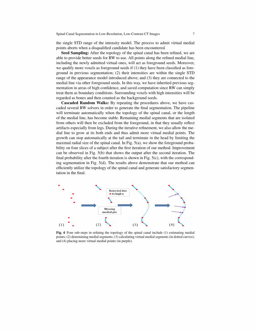
ing all segments of the medial line given the tentative segmentation, we interleavethem into a single connected curve. Fig. 4 illustrates the four sub-steps to refine thetopology of the spinal canal with regard to its medial line. Based on tentative seg-mentation (including outputs from voxelwise classification), we calculate the me-dial point of foreground voxels on each transverse slice in Fig. 4(1). The medialpoint is defined to have the least sum of distances to all other foreground voxelson each slice. Assuming that the medial line connects all medial points, we thenconnect the medial points into several segments in Fig. 4(2). The medial line maybreak into several segments since medial points can be missing. Also certain me-dial point would be rejected as outlier if it incurs too high curvature to the medialline. With all computed segments, we interleave them by filling gaps with smoothvirtual segments (as dotted curves) in Fig. 4(3). Each virtual segment c(s) mini-mizes

∫‖∇2c(s)‖2ds to keep smooth as s ∈ [0,1] for normalized arc-length. The

stationary solution to the above holds when ∇4c(s) = 0, and the Cauchy boundaryconditions are defined by both two ends of the virtual segment as well as tangentdirections at the ends. Though the numerical solution is non-unique, we apply thecubic Bzier curve for fast estimation of the virtual segment. For a certain virtualsegment, we denote its ends as P0 and P3. An additional control point P1 is placedso that the direction from P0 to P1 is identical to the tangent direction at P0. Sim-ilarly, we can define P2 according to P3 and the associated tangent direction. Wefurther require that the four control points are equally spaced. The virtual segmentis c(s) = (1− s)3P0 +3(1− s)2sP1 +3(1− s)s2P2 + s3P3.

After predicting the virtual segment in Fig. 4(3), we finally place more virtualmedial points along the virtual segment. Besides the subject-specific geometry con-straints to keep the virtual segments smooth, we further incorporate appearance cri-terion in Fig. 4(4). Upon all existing medial points (red dots), we calculate theirintensity mean and the standard deviation (STD). The univariate Gaussian intensitymodel allows us to examine whether a new voxel is highly possible to be foregroundgiven its simple appearance value. In particular, we start from both two ends of eachvirtual segment, and admit virtual medial point (purple dot) if its intensity is within

Fig. 3 With foreground seeds (in red) and background seeds (in green) (a), the calculated probabil-ities (b) and the corresponding binary segmentation (c) are not satisfactory. However, by manuallyplacing more seeds (d), the segmentation results (e-f) are improved significantly.


the single STD range of the intensity model. The process to admit virtual medialpoints aborts when a disqualified candidate has been encountered.

Seed Sampling: After the topology of the spinal canal has been refined, we areable to provide better seeds for RW to use. All points along the refined medial line,including the newly admitted virtual ones, will act as foreground seeds. Moreover,we qualify more voxels as foreground seeds if (1) they have been classified as fore-ground in previous segmentation; (2) their intensities are within the single STDrange of the appearance model introduced above; and (3) they are connected to themedial line via other foreground seeds. In this way, we have inherited previous seg-mentation in areas of high confidence, and saved computation since RW can simplytreat them as boundary conditions. Surrounding voxels with high intensities will beregarded as bones and then counted as the background seeds.

Cascaded Random Walks: By repeating the procedures above, we have cas-caded several RW solvers in order to generate the final segmentation. The pipelinewill terminate automatically when the topology of the spinal canal, or the lengthof the medial line, has become stable. Remaining medial segments that are isolatedfrom others will then be excluded from the foreground, in that they usually reflectartifacts especially from legs. During the iterative refinement, we also allow the me-dial line to grow at its both ends and thus admit more virtual medial points. Thegrowth can stop automatically at the tail and terminate in the head by limiting themaximal radial size of the spinal canal. In Fig. 5(a), we show the foreground proba-bility on four slices of a subject after the first iteration of our method. Improvementcan be observed in Fig. 5(b) that shows the output after the second iteration. Thefinal probability after the fourth iteration is shown in Fig. 5(c), with the correspond-ing segmentation in Fig. 5(d). The results above demonstrate that our method canefficiently utilize the topology of the spinal canal and generate satisfactory segmen-tation in the final.

Fig. 4 Four sub-steps in refining the topology of the spinal canal include (1) estimating medialpoints; (2) determining medial segments; (3) calculating virtual medial segments (in dotted curves);and (4) placing more virtual medial points (in purple).


3 Experimental Result

We have conducted a study on 110 individual images from eight medical sites, asthe largest scale reported in the literature, to verify the capability of our method.The training data are not used for the sake of testing. Even though the image qualityof our data is low and the appearance variation is extremely high, we successfullygenerate good segmentation results on all datasets by our method with a fixed con-figuration. Sagittal views of segmentation results for 4 randomly selected subjectsare shown in Fig. 6(a)-(d), respectively. In Fig. 6(e)-(g), we also show the segmen-tation result in 3 coronal slices for the extreme case in Fig. 1(b). This patient isunder influences from severe diseases, which cause an unusual twist to the spine.However, though the topology of the spinal canal under consideration is abnormal,our method is still capable to well segment the whole structure. All results aboveconfirm that our method is robust in dealing with the challenging data.

(a)

(c) (d)

(b)

0 1 0 1

0 1

Fig. 5 Panels (a)-(c) show foreground probability on 4 consecutive slices of a certain subject outputafter the first, second, and the final (fourth) iteration, respectively. The binary segmentation in (d)is corresponding to the final probability in (c).


We have further manually annotated 20 datasets for quantitative evaluation. Forthe manually delineated parts, the Dice overlapping ratio between the segmenta-tion of our method and the ground truth reaches 92.791.55%. By visual inspec-tion, robust and good segmentation results are achieved on all 110 datasets, espe-cially including many highly pathological cases. Note that to deal with image datawith severe pathologies is not addressed and validated in the previous literature[2, 3, 4, 5, 7].

Our method achieves final segmentation in 2-5 iterations for all datasets, andtypically costs 20-60 seconds per volume depending on the image size. With moresophisticated RW method that is better designed for editing seeds [12], the speedperformance of our method can be further improved.

(a) (b) (c) (d)

(e) (f) (g)

Fig. 6 Panels (a)-(d) show segmentation results (in sagittal views) on 4 randomly selected images.Coronal views of the segmentation results on an extreme case, whose spine twists due to diseases,are shown in (e)-(g).


4 Discussion

In this work, an automatic method to segment spinal canals from low-quality CTimages is proposed. With initial seeds provided by PBT-based classification, weintroduce topology constraints into segmentation via RW. Our iterative optimiza-tion has successfully enhanced the capability of RW in dealing with tubular spinalcanals, in that the boundary conditions can be improved to guarantee better segmen-tation results. Our large-scale evaluation shows that the proposed method is highlyaccurate and robust even if the datasets are very diverse and challenging.

References

1. T. Klinder, J. Ostermann, M. Ehm, A. Franz, R. Kneser, C. Lorenz, Medical Image Analysis13(3), 471 (2009)

2. N. Archip, P.J. Erard, M. Egmont-Petersen, J.M. Haefliger, J.F. Germond, Medical Imaging,IEEE Transactions on 21(12), 1504 (2002)

3. S.S.C. Burnett, G. Starkschall, C.W. Stevens, Z. Liao, Medical Physics 31(2), 251 (2004)4. G. Karangelis, S. Zimeras, in Bildverarbeitung fur die Medizin 2002, ed. by M. Meiler,

D. Saupe, F. Kruggel, H. Handels, T. Lehmann (Springer Berlin Heidelberg, 2002), pp. 370–373

5. L. Nyul, J. Kanyo, E. Mate, G. Makay, E. Balogh, M. Fidrich, A. Kuba, in Computer Anal-ysis of Images and Patterns, vol. 3691, ed. by A. Gagalowicz, W. Philips (Springer BerlinHeidelberg, 2005), vol. 3691, pp. 456–463

6. M. Kass, A. Witkin, D. Terzopoulos, International Journal of Computer Vision 1(4), 321(1988)

7. J. Yao, S. O’Connor, R. Summers, in Biomedical Imaging: Nano to Macro, 2006. 3rd IEEEInternational Symposium on (2006), pp. 390–393

8. D. Cremers, M. Rousson, R. Deriche, International Journal of Computer Vision 72(2), 195(2007)

9. L. Grady, Pattern Analysis and Machine Intelligence, IEEE Transactions on 28(11), 1768(2006)

10. D. Wu, D. Liu, Z. Puskas, C. Lu, A. Wimmer, C. Tietjen, G. Soza, S. Zhou, in ComputerVision and Pattern Recognition (CVPR), 2012 IEEE Conference on (2012), pp. 980–987

11. Z. Tu, in Computer Vision, 2005. ICCV 2005. Tenth IEEE International Conference on, vol. 2(2005), vol. 2, pp. 1589–1596 Vol. 2

12. S. Andrews, G. Hamarneh, A. Saad, in Medical Image Computing and Computer-AssistedIntervention – MICCAI 2010, vol. 6363, ed. by T. Jiang, N. Navab, J. Pluim, M. Viergever(Springer Berlin Heidelberg, 2010), vol. 6363, pp. 9–16

Automatic and Reliable Segmentation of Spinal...

Documents

Transcript of Automatic and Reliable Segmentation of Spinal...