GeoinformaticaDOI 10.1007/s10707-008-0046-3

Automatic and Accurate Extraction of RoadIntersections from Raster Maps

Yao-Yi Chiang · Craig A. Knoblock · Cyrus Shahabi ·Ching-Chien Chen

Received: 23 June 2006 / Revised: 19 December 2007 /Accepted: 4 February 2008© Springer Science + Business Media, LLC 2008

Abstract Since maps are widely available for many areas around the globe, theyprovide a valuable resource to help understand other geospatial sources such as toidentify roads or to annotate buildings in imagery. To utilize the maps for under-standing other geospatial sources, one of the most valuable types of information weneed from the map is the road network, because the roads are common featuresused across different geospatial data sets. Specifically, the set of road intersectionsof the map provides key information about the road network, which includes thelocation of the road junctions, the number of roads that meet at the intersections(i.e., connectivity), and the orientations of these roads. The set of road intersectionshelps to identify roads on imagery by serving as initial seed templates to locate roadpixels. Moreover, a conflation system can use the road intersections as referencefeatures (i.e., control point set) to align the map with other geospatial sources, such as

This work is based on an earlier paper: Automatic Extraction of Road Intersectionsfrom Raster Maps, in Proceedings of the 13th annual ACM International Symposiumon Geographic Information Systems, Pages: 267–276, ©ACM, 2005.http://doi.acm.org/10.1145/1097064.1097102.

Y.-Y. Chiang (B) · C. A. KnoblockDepartment of Computer Science and Information Sciences Institute,University of Southern California, Marina del Rey, CA 90292 USAe-mail: yaoyichi@isi.edu

C. A. Knoblocke-mail: knoblock@isi.edu

C. ShahabiComputer Science Department, University of Southern California,SAL 300, Los Angeles, CA 90089-0781, USAe-mail: shahabi@usc.edu

C.-C. ChenGeosemble Technologies, 2041 Rosecrans Ave. Suite 245 El Segundo, CA 90245 USAe-mail: jchen@geosemble.com

Geoinformatica

aerial imagery or vector data. In this paper, we present a framework for automaticallyand accurately extracting road intersections from raster maps. Identifying the roadintersections is difficult because raster maps typically contain much informationsuch as roads, symbols, characters, or even contour lines. We combine a varietyof image processing and graphics recognition methods to automatically separateroads from the raster map and then extract the road intersections. The extractedinformation includes a set of road intersection positions, the road connectivity, androad orientations. For the problem of road intersection extraction, our approachachieves over 95% precision (correctness) with over 75% recall (completeness) onaverage on a set of 70 raster maps from a variety of sources.

Keywords Raster map · Road layer · Road intersection · Imagery · Conflation ·Fusion · Vector data · Geospatial data integration

1 Introduction

Humans have a very long history of using maps. Fortunately, due to the widespreaduse of Geographic Information System and the availability of high quality scanners,we can now obtain many maps in raster format from various sources, such asdigitally scanned maps from USGS Topographic Maps on Microsoft Terraserver1 orcomputer generated maps from U.S Census Bureau2 (TIGER/Line Maps), GoogleMaps,3 Yahoo Maps,4 MapQuest Maps,5 etc. Not only are the raster maps readilyaccessible compared to other geospatial data (e.g., vector data), but they provide veryrich information, such as road names, landmarks, or even contour lines. Considerthe fact that road maps are generally the most frequently used map type and theroad layers commonly exist across many different geospatial data sources, the roadnetwork can be used to fuse a map with other geospatial data. In particular, insteadof extracting the whole road network, road intersection templates (i.e., the positionsof the road intersections, the road connectivity and orientations) provide the basicelements of the road layout and are comparatively easy to extract. For example, theroad intersection templates can be used to extract roads from other sources, such asaerial images [13]. As shown in Fig. 1, without using the whole road network, theextracted road intersection templates can be used as seed templates to extract theroads from the imagery of Tehran, Iran where we have limited access to the vectordata. Moreover, since the layout of a set of road intersections within a certain area isusually unique, we can utilize the road intersections as the “fingerprint” of the rastermap to determine the extent of a map that is not georeferenced [9]; and further, theroad intersections can be used as feature points to align the raster map with othergeospatial sources [5]. For example, Fig. 2a shows a hybrid view of Tehran, Iran fromGoogle Map where only major roads are shown with labels. By matching the layout

1http://terraserver-usa.com/2http://tiger.census.gov/cgi-bin/mapsurfer3http://map.google.com4http://map.yahoo.com5http://www.mapquest.com

Geoinformatica

Fig. 1 Use the extracted roadintersections as seed templatesto extract roads from imagery

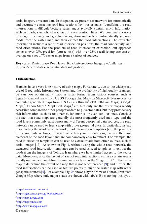
of road intersections from a tourist map found on the Internet shown in Fig. 2b to thecorresponding layout on the satellite imagery, we can create a enhanced integratedrepresentation of the maps and imagery as shown in Fig. 3.

Fig. 2 The integration ofimagery from Google Map anda tourist map (Tehran, Iran).a The Google Map hybridview. b The tourist mapin Farsi

Geoinformatica

Fig. 3 The integration of imagery from Google Map and a tourist map (Tehran, Iran)

Automatic extraction of road intersections is difficult due(e.g., map geocoordi-nates, scales, legend, original vector data, etc) and also the great complexity of maps.For example, for a Google Map snapshot in an article or an evacuation map postedon a wildfire news website, there is no uniform metadata or auxiliary informationthat can be automatically found and parsed to help utilize the map without humanintervention. In addition, maps typically contain multiple layers of roads, buildings,symbols, characters, etc. People interpret the maps by examining the map contextsuch as road labels or looking for the map legends, which is a difficult task formachines. To overcome these problems, we present a framework, which works onthe pixel level and utilizes the distinctive geometric properties of road lines andintersections to automatically extract road intersections from raster maps. The inputsof our approach are raster maps from a variety of sources without any auxiliaryinformation such as the color of the roads, vector data, or legend information, etc.

Geoinformatica

ba

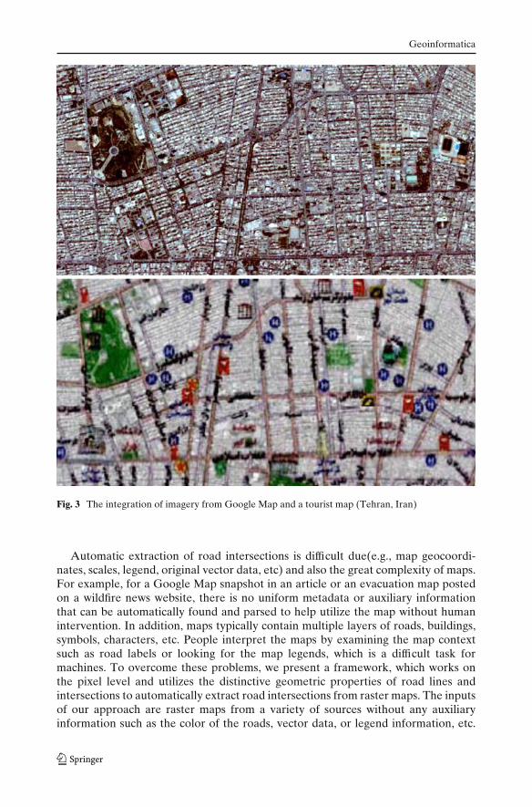
Fig. 4 Example input raster maps. a USGS Topographic Map. b TIGER/Line Map

Two examples of the input raster maps are shown in Fig. 4. The outputs are thepositions of the road intersection points, the number of roads that meet at eachintersection as well as the orientation of each intersected road.

For the problem of automatic extraction of road intersections from raster maps,much of the previous work provides partial solutions [2], [6], [10], [11], [15]–[18],[24]–[26]. A majority of the work [2], [6], [15], [26] focuses on extracting text frommaps and the road lines are typically ignored in the process. Others such as Salvatoreand Guitton [24] work on extracting and rebuilding the lines; however they relyheavily on prior learned colors to separate the lines for specific data sets, which is notgenerally useful in our automatic process. Habib et al. [11] assume the maps containonly roads, and work on road lines directly to extract intersections. These previousapproaches require manual interactions as they provide only partial solutions; and webuild on some of the previous work in our framework to solve specific sub-problems.For example, to extract road lines from the foreground pixels, we incorporate Caoet al.’s algorithm [6] as the first step to remove small connected objects such ascharacters from the map. Our approach is a complete solution that does not rely onprior knowledge of the input raster maps.

This paper is based on our earlier paper [7] of this work, and the new contributionsof this paper are as follows:

1. We describe our approach in more detail (Section 2).2. We describe how we utilize the Localized Template Matching (LTM) [4] to

improve our algorithm (Section 2.6.3). We also report the similarity valuegenerated by LTM to evaluate the quality of the extracted road intersectiontemplates (i.e., the road intersection, connectivity and orientations) (Section 3).

3. We present a more extensive set of experiments testing our approach on moremap sources, and we also report the computation time with respect to the numberof foreground pixels on a map (Section 3).

Geoinformatica

4. We report our precision, recall, and F-measure on different positional accuracylevels (Section 3).

5. We report the results of a comparison on the same set of map sources using theapproach in this paper against the approaches in our previous work [3] and anearlier paper of this work [7] (Section 3).

The remainder of this paper is organized as follows. Section 2 describes ourapproach to automatically extract road intersections. Section 3 reports on ourexperimental results. Section 4 discusses the related work and Section 5 presents theconclusion and future work.

2 Automatic road intersection extraction

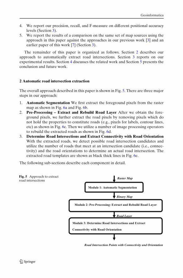
The overall approach described in this paper is shown in Fig. 5. There are three majorsteps in our approach:

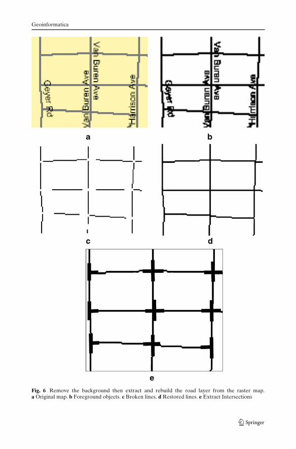
1. Automatic Segmentation We first extract the foreground pixels from the rastermap as shown in Fig. 6a and Fig. 6b.

2. Pre-Processing – Extract and Rebuild Road Layer After we obtain the fore-ground pixels, we further extract the road pixels by removing pixels which donot hold the properties to constitute roads (e.g., pixels for labels, contour lines,etc) as shown in Fig. 6c. Then we utilize a number of image processing operatorsto rebuild the extracted roads as shown in Fig. 6d.

3. Determine Road Intersections and Extract Connectivity with Road OrientationWith the extracted roads, we detect possible road intersection candidates andutilize the number of roads that meet at an intersection candidate (i.e., connec-tivity) and the road orientations to determine an actual road intersection. Theextracted road templates are shown as black thick lines in Fig. 6e.

The following sub-sections describe each component in detail.

Fig. 5 Approach to extractroad intersections

Module 3: Determine Road Intersections and Extract

Connectivity with Road Orientation

Road Intersection Points with Connectivity and Orientation

Module 2: Pre-Processing: Extract and Rebuild Road Layer

Road Layer

Binary Map

Module 1: Automatic Segmentation

Raster Map

Geoinformatica

Fig. 6 Remove the background then extract and rebuild the road layer from the raster map.a Original map. b Foreground objects. c Broken lines. d Restored lines. e Extract Intersections

Geoinformatica

2.1 Automatic segmentation

In this step, the input is a raster map, and our goal is to extract the foregroundpixels from the map. We utilize a technique called segmentation with automaticallygenerated thresholds to separate the foreground from the background pixels. Manysegmentation methods are discussed and proposed for various applications [23],and we implement a method that analyze the shape of the grayscale histogram andclassify the histogram clusters based on their sizes. Our implementation is based onour observations of the color usage on raster maps, which are:

1. The background colors of raster maps have a dominant number of pixels; andthe number of foreground pixels are significantly smaller than the number offoreground background pixels.

2. The foreground colors have high contrast against the background colors.

The first step is to convert the original input raster map to an 8-bit grayscale(i.e., 256 luminosity levels) image as shown in Fig. 7a. The conversion is done bycomputing the average value of the red, green and blue strength of each pixel for thegrayscale level. The grayscale histogram of Fig. 7a is shown in Fig. 8. In the histogram,the X-axis represents the luminosity level; from 0 (black) to 255 (white), and theY-axis has the histogram values that represent the number of pixels for eachluminosity level. We then partition the histogram into luminosity clusters and labelthe clusters as either background or foreground clusters.

Since the background colors have a dominant number of pixels, we start fromsearching for the the global maximum on the histogram value to identify the firstbackground cluster. As shown in Fig. 8, we first find PEAK 1, then we check whether

ba

Fig. 7 Before and after automatic segmentation (USGS Topographic Map). a Before (grayscalemap). b After (binary map)

Geoinformatica

Fig. 8 Find Cluster 1’s left bound threshold using the triangle method

PEAK 1 is closer to 255 (white) or 0 (black) in the histogram to determine whichpart in the histogram (i.e., the portion of histogram to the left or right of PEAK 1)contains the foreground colors. If the peak is closer to 255, such as PEAK 1, 255(white) is used as the right boundary of the first background cluster. This is becausethe foreground colors generally have high contrast against the background colors.For example, if a light gray color of luminosity 200 is used as the background, itis common to find the foreground colors spread in the histogram between 0 to 200instead of between 200 to 255. As a result, for Cluster 1 in Fig. 8, we identify 255 as itsright boundary, and its left boundary is located using the triangle method proposedby Zack [27], which will be discussed latter. On the other hand, if PEAK 3 is theglobal maximum, we will use 0 as its left boundary, and its right boundary is thenlocated using the triangle method.

After we find the first cluster, we search for next peak and use the triangle methodto locate the cluster’s left and right boundaries until every luminosity level in thehistogram belongs to some cluster. Any clustering algorithm could be used to findthe cluster boundary, and we use the triangle method proposed by Zack [27] forits simplicity. As shown in Fig. 8, to find the left or right boundary, we construct aline called triangle line between the peak and the 0 or 255 end point and computethe distance between each Y-value and the triangle line. The luminosity level thathas its Y-value under the triangle line and has the maximum distance is the cluster’sleft/right boundary as the dotted line indicates in Fig. 8. If every luminosity level hasits Y-value above the triangle line, then the 0 or 255 end point is used as the left orright boundary of the cluster. For example, if we try to find the left boundary forCluster 3 using the triangle method, we will find that every Y-value on the left ofPEAK 3 is above the triangle line, so 0 is used for the left boundary of Cluster 3.

Geoinformatica

Table 1 Number of pixels ineach cluster Cluster 1 Cluster 2 Cluster 3

Cluster pixels 316846 237876 85278Cluster pixels / total pixels 50% 37% 13%

In our example, Cluster 1 is first classified as the first background cluster. Theforeground colors usually have high contrast against the background colors, so thecluster which is the farthest from the first background cluster in the histogram isthe first foreground cluster (i.e., Cluster 3 in our example). For the remaining clusters,we compare the number of pixels in each cluster to the background cluster andthe foreground cluster. If the number of pixels of a cluster is closer to the numberof pixels of the background clusters than foreground clusters, it is classified as abackground cluster; otherwise it is a foreground cluster. For example, as shown inTable 1, the number of pixels in Cluster 2 is closer to Cluster 1(background) thanCluster 3 (foreground), so Cluster 2 is classified as a background cluster. The ideais, if a cluster uses as many pixels as any of the background cluster, we do not wantto include it in our result for two reasons. First, the cluster could be another colorused in the background. Second, the cluster could be the color used to fill up largeobjects on the map such as parks, lakes, etc. Since our goal is to look for road linesin the foreground pixels, the cluster should be discarded in either case. After eachcluster is classified as background or foreground, we remove the background clusters(i.e., convert the color of pixels in background clusters to white). An example of theresulting binary image is shown in Fig. 7b.

There is no universal solution for the automatic segmentation problem. An edgedetector is sometimes used instead of thresholding [11]; however, the edge detectoris sensitive to noise, which makes it difficult to use for our approach. Moreover, withthe presence of characters, the edge detector makes the resulting characters biggerthan the original ones since the edge detector produces two edges for a characterline segment. Big characters have more overlap with road lines and hence severelysabotage the results of the next step that extract and rebuild the road layer. On theother hand, a simple thresholding algorithm can be applied to a wide-range of mapsources.

2.2 Pre-processing—extracting and rebuilding road layers

After we separate the foreground from the background pixels, we have a binaryraster map that contains multiple layers such as roads, labels, etc. In this module, weextract and rebuild the road layer from the binary map. In order to extract the roadlayer, we need to remove the objects that do not possess the geometric properties ofroads. Without losing generality, our assumptions about roads on raster maps are:

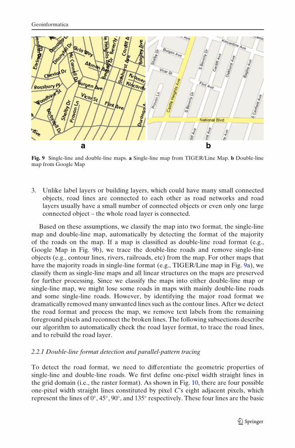
1. Road lines are straight within a small distance (i.e., several meters).2. The linear structures (i.e., lines) in a map are mainly roads. The majority of

the roads share the same road format—single-line roads or double-line roads,and the double-line roads have the same road width within a map. Examples ofsingle-line and double-line maps are shown in Fig. 9

Geoinformatica

Fig. 9 Single-line and double-line maps. a Single-line map from TIGER/Line Map. b Double-linemap from Google Map

3. Unlike label layers or building layers, which could have many small connectedobjects, road lines are connected to each other as road networks and roadlayers usually have a small number of connected objects or even only one largeconnected object – the whole road layer is connected.

Based on these assumptions, we classify the map into two format, the single-linemap and double-line map, automatically by detecting the format of the majorityof the roads on the map. If a map is classified as double-line road format (e.g.,Google Map in Fig. 9b), we trace the double-line roads and remove single-lineobjects (e.g., contour lines, rivers, railroads, etc) from the map. For other maps thathave the majority roads in single-line format (e.g., TIGER/Line map in Fig. 9a), weclassify them as single-line maps and all linear structures on the maps are preservedfor further processing. Since we classify the maps into either double-line map orsingle-line map, we might lose some roads in maps with mainly double-line roadsand some single-line roads. However, by identifying the major road format wedramatically removed many unwanted lines such as the contour lines. After we detectthe road format and process the map, we remove text labels from the remainingforeground pixels and reconnect the broken lines. The following subsections describeour algorithm to automatically check the road layer format, to trace the road lines,and to rebuild the road layer.

2.2.1 Double-line format detection and parallel-pattern tracing

To detect the road format, we need to differentiate the geometric properties ofsingle-line and double-line roads. We first define one-pixel width straight lines inthe grid domain (i.e., the raster format). As shown in Fig. 10, there are four possibleone-pixel width straight lines constituted by pixel C’s eight adjacent pixels, whichrepresent the lines of 0◦, 45◦, 90◦, and 135◦ respectively. These four lines are the basic

Geoinformatica

Fig. 10 Basic single-line roadelements

elements to constitute other straight lines with various slopes starting from pixel C.For example, in Fig. 11, to represent a 30◦ line, one of the basic elements, a 45◦line segment, is drawn in black, then additional gray pixels is added to tilt the line.Hence, by identifying these basic elements, we can identify straight lines in single-line format.Based on the four basic elements, if the pixel C is on a double-line roadsshown in Fig. 12, there are eight different parallel-patterns of double-line roads (i.e.,the dashed cells are possible parallel lines). If we can detect any of the eight patternsfor a given foreground pixel, we classify the pixel as a double-line road pixel. Asshown in Fig. 12, we draw a cross at the pixel C using the size of the road width; andthe cross locates at least two road line pixels on each pattern, one at the horizontaldirection and the other one at the vertical direction. Therefore, if we know the road

Fig. 11 A 45◦ basic element(black) in the 30◦ line segment(both black and gray)

Geoinformatica

Fig. 12 Basic double-line roadelements

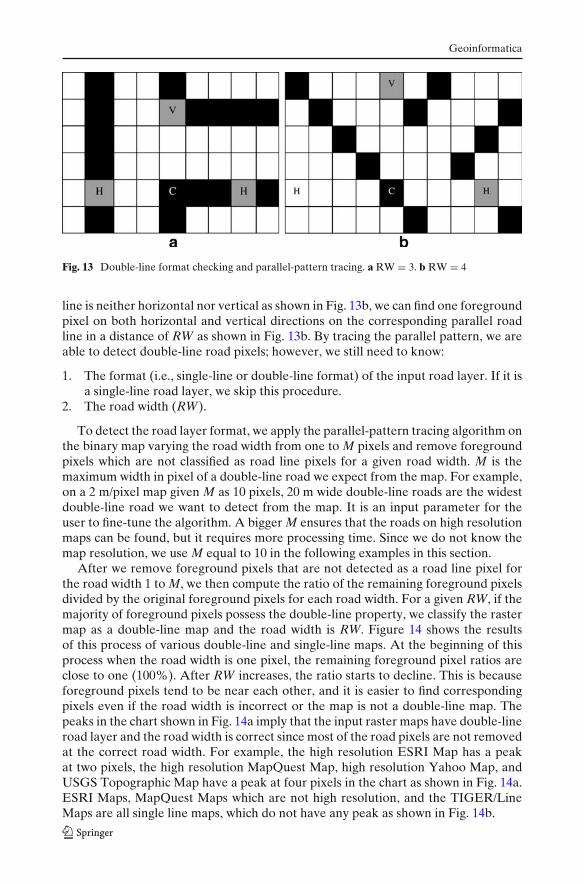
width, we can determine whether a foreground pixel is on a double-line road layerby searching for the corresponding foreground pixels within a distance of road width(RW)6 in vertical and horizontal directions to find the parallel pattern. Two examplesare shown in Fig. 13. If a foreground pixel is on a horizontal or vertical road lineas shown in Fig. 13a, we can find two foreground pixels along the orientation ofthe road line within a distance of RW and at least another foreground pixel on thecorresponding parallel road line in a distance of RW. If the orientation of the road

6RW is used in this paper as a variable representing the road width in pixels.

Geoinformatica

Fig. 13 Double-line format checking and parallel-pattern tracing. a RW = 3. b RW = 4

line is neither horizontal nor vertical as shown in Fig. 13b, we can find one foregroundpixel on both horizontal and vertical directions on the corresponding parallel roadline in a distance of RW as shown in Fig. 13b. By tracing the parallel pattern, we areable to detect double-line road pixels; however, we still need to know:

1. The format (i.e., single-line or double-line format) of the input road layer. If it isa single-line road layer, we skip this procedure.

2. The road width (RW).

To detect the road layer format, we apply the parallel-pattern tracing algorithm onthe binary map varying the road width from one to M pixels and remove foregroundpixels which are not classified as road line pixels for a given road width. M is themaximum width in pixel of a double-line road we expect from the map. For example,on a 2 m/pixel map given M as 10 pixels, 20 m wide double-line roads are the widestdouble-line road we want to detect from the map. It is an input parameter for theuser to fine-tune the algorithm. A bigger M ensures that the roads on high resolutionmaps can be found, but it requires more processing time. Since we do not know themap resolution, we use M equal to 10 in the following examples in this section.

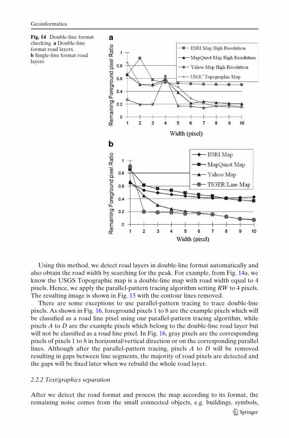
After we remove foreground pixels that are not detected as a road line pixel forthe road width 1 to M, we then compute the ratio of the remaining foreground pixelsdivided by the original foreground pixels for each road width. For a given RW, if themajority of foreground pixels possess the double-line property, we classify the rastermap as a double-line map and the road width is RW. Figure 14 shows the resultsof this process of various double-line and single-line maps. At the beginning of thisprocess when the road width is one pixel, the remaining foreground pixel ratios areclose to one (100%). After RW increases, the ratio starts to decline. This is becauseforeground pixels tend to be near each other, and it is easier to find correspondingpixels even if the road width is incorrect or the map is not a double-line map. Thepeaks in the chart shown in Fig. 14a imply that the input raster maps have double-lineroad layer and the road width is correct since most of the road pixels are not removedat the correct road width. For example, the high resolution ESRI Map has a peakat two pixels, the high resolution MapQuest Map, high resolution Yahoo Map, andUSGS Topographic Map have a peak at four pixels in the chart as shown in Fig. 14a.ESRI Maps, MapQuest Maps which are not high resolution, and the TIGER/LineMaps are all single line maps, which do not have any peak as shown in Fig. 14b.

Geoinformatica

Fig. 14 Double-line formatchecking. a Double-lineformat road layers.b Single-line format roadlayers

Using this method, we detect road layers in double-line format automatically andalso obtain the road width by searching for the peak. For example, from Fig. 14a, weknow the USGS Topographic map is a double-line map with road width equal to 4pixels. Hence, we apply the parallel-pattern tracing algorithm setting RW to 4 pixels.The resulting image is shown in Fig. 15 with the contour lines removed.

There are some exceptions to use parallel-pattern tracing to trace double-linepixels. As shown in Fig. 16, foreground pixels 1 to 8 are the example pixels which willbe classified as a road line pixel using our parallel-pattern tracing algorithm, whilepixels A to D are the example pixels which belong to the double-line road layer butwill not be classified as a road line pixel. In Fig. 16, gray pixels are the correspondingpixels of pixels 1 to 8 in horizontal/vertical direction or on the corresponding parallellines. Although after the parallel-pattern tracing, pixels A to D will be removedresulting in gaps between line segments, the majority of road pixels are detected andthe gaps will be fixed later when we rebuild the whole road layer.

2.2.2 Text/graphics separation

After we detect the road format and process the map according to its format, theremaining noise comes from the small connected objects, e.g. buildings, symbols,

Geoinformatica

Fig. 15 USGS Topographic Map before and after parallel-pattern tracing. a Before. b After

characters, etc. The small connected objects tend to be near each other on the rastermaps, such as characters that are close to each other to form strings, and buildingsthat are close to each other on a street block. The text/graphics separation algo-rithms [2], [6], [10], [15]–[18], [25], [26] are very suitable for grouping and removingthese types of objects. The text/graphics separation algorithms start by identifyingsmall connected objects and then use various algorithms to search neighborhoodobjects in order to build object groups [25].

We apply Cao et al.’s algorithm described in [6] for text/graphics separation.Their algorithm first removes small connected objects that do not overlap with otherobjects in the raster map as shown in Fig. 17b and then checks the length of eachremaining line segment to determine if the line segment belongs to a graphic object.If a line segment is longer than a preset threshold, it is considered a graphic object(i.e., a line); otherwise, it is a text object (i.e., not a line). The identified text objectsare shown in Fig. 17c, and the final result after text/graphics separation is show inFig. 17d. The broken road lines are inevitable after the removal of those objectstouching lines, and we can reconnect them when rebuilding the road layer.

With Cao et al.’s algorithm, we need to specify several parameters for thegeometric properties of the characters, such as the size of one character and the

Geoinformatica

3 4 4 4

A C

B D

3 3 3 4 5 5

2 6 7

3 5

2 2 6 6 6 7 8 7 7

1

2 8 8

1 1

Fig. 16 The exceptions in double-line format checking and parallel-pattern tracing (white cells arebackground pixels)

maximum length of a word. Since we do not have the information to setup thealgorithm for different maps, we first conduct several initial tests on a disjoint set ofmaps and select a set of parameters to be used in our experiments. Our experimentshows that Cao et al.’s algorithm is very robust since the input parameters do nothave to be exact. Also, the characters sizes of many computer generated raster mapsvary in a small range for users to read the map comfortably. For example, the mapsfrom Google Map at different zooming level and maps from Yahoo Map have similarsizes of street labels. For the scanned maps, the characters could be enormouslyenlarged/shrunk depending on the scan resolution; and the text/graphics separationalgorithm will fail given that no additional geometric properties of the characters areprovided. However, scanned maps usually are scaled down for user-friendly viewingor to be displayed on the Internet, so it is not common that the input map is ascanned maps with a extremely high/low scan resolution and enormously large/smallcharacters.

2.2.3 Rebuilding road layers: binary morphological operators

In the previous steps, we extracted the road layer and created broken lines during theextraction. In this step, we utilize the binary morphological operators to reconnectthe lines and fix the gaps. Binary morphological operators are easily implementedusing hit-or-miss transformations with various size masks [19], and are often used invarious document analysis algorithms as fundamental operations [1]. The hit-or-misstransformation is performed in our approach as follows. We use 3-by-3 binary masksto scan over the input binary images. If the masks match the underlying pixels, it is a“hit”; otherwise, it is a “miss”. Each operator uses different masks to perform hit-or-miss transformations and performs different actions as a result of a “hit” or “miss”.We describe each operator in turn.

2.3 Binary dilation

The basic effect of a binary dilation operator is to expand the region of foregroundpixels [19] and we use it to thicken the lines and reconnect adjacent pixels. As

Geoinformatica

Fig. 17 TIGER/Line map before and after text/graphics separation. a Binary TIGER/Line map.b Remove small connected components. c Identify non-line objects. d After text/graphics separation

shown in Fig. 18, if a background pixel has any foreground pixel in its eight adjacentpixels (i.e., a “hit”), it is filled up as a foreground pixel (i.e., the action resultingfrom the “hit”). For example, Fig. 19 shows that after two iterations, the generaldilation operator fixes the gap between two broken lines. Moreover, if the roads arein double-line format, the two parallel lines are combined to a single line after the

Fig. 18 Dilation (black cellsare foreground pixels)

Geoinformatica

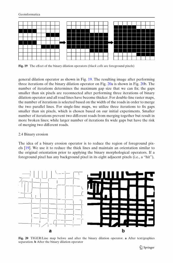
Fig. 19 The effect of the binary dilation operators (black cells are foreground pixels)

general dilation operator as shown in Fig. 19. The resulting image after performingthree iterations of the binary dilation operator on Fig. 20a is shown in Fig. 20b. Thenumber of iterations determines the maximum gap size that we can fix; the gapssmaller than six pixels are reconnected after performing three iterations of binarydilation operator and all road lines have become thicker. For double-line raster maps,the number of iterations is selected based on the width of the roads in order to mergethe two parallel lines. For single-line maps, we utilize three iterations to fix gapssmaller than six pixels, which is chosen based on our initial experiments. Smallernumber of iterations prevent two different roads from merging together but result inmore broken lines; while larger number of iterations fix wide gaps but have the riskof merging two different roads.

2.4 Binary erosion

The idea of a binary erosion operator is to reduce the region of foreground pix-els [19]. We use it to reduce the thick lines and maintain an orientation similar tothe original orientation prior to applying the binary morphological operators. If aforeground pixel has any background pixel in its eight adjacent pixels (i.e., a “hit”),

Fig. 20 TIGER/Line map before and after the binary dilation operator. a After text/graphicsseparation. b After the binary dilation operator

Geoinformatica

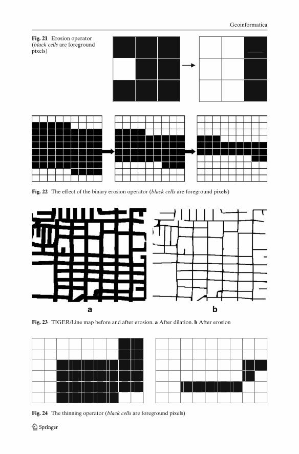
Fig. 21 Erosion operator(black cells are foregroundpixels)

Fig. 22 The effect of the binary erosion operator (black cells are foreground pixels)

Fig. 23 TIGER/Line map before and after erosion. a After dilation. b After erosion

Fig. 24 The thinning operator (black cells are foreground pixels)

Geoinformatica

it is converted to a background pixel (i.e., the action resulting from the “hit”) asshown in Fig. 21. For example, Fig. 22 shows that after two iterations, the generalerosion operator reduces the width of the thick lines. The resulting image afterperforming two iterations of the binary erosion operator on Fig. 23a is shown inFig. 23b.

2.5 Thinning

After applying the binary dilation and erosion operators, we have road layerscomposed from road lines with various widths. But we need the road lines to haveexactly one pixel width to detect interest points and the connectivity in the nextstep, and the thinning operator can produce the one pixel width results. The effectof the thinning operator is shown in Fig. 24. We do not use the thinning operatorright after the binary dilation operator because the binary erosion operator hasthe opposite affect to the binary dilation operator, which prevent the orientationof road lines near the intersections from being distorted, as shown in Fig. 25. Weutilize a generic thinning operator that is a conditional erosion operator with anextra confirmation step [19]. The first step of the thinning operator is to mark everyforeground pixel that connects to one or more background pixels (i.e., the same ideaas the binary erosion operator) as candidate to be converted to the background.Then the confirmation step checks if the conversion of the candidate will cause anydisappearance of original line branches to ensure the basic structure of the originalobjects will not be compromised. The resulting image after performing the thinningoperator on Fig. 26a is shown in Fig. 26b.

2.6 Determine road intersections, connectivity, and orientation

In this step, we automatically extract road intersections, connectivity (i.e., thenumber of roads that meet at an intersection), and the orientation of the roads inter-secting at each intersection from the road layer. In addition, we utilize the extractedinformation (i.e., the position of the extracted intersection point, connectivity, andorientation) and the original map to verify and improve the results in the last step ofthis module.

Fig. 25 The results after thinning with and without erosion. a After dilation. b Without erosion.c With erosion

Geoinformatica

Fig. 26 TIGER/Line map before and after thinning. a After erosion. b After thinning

2.6.1 Detection of road intersection candidates

With the roads from the preprocessing steps, we need to locate possible roadintersection points. A road intersection point is a point at which more than two linesmeet with different tangents. To detect possible intersection points, we start by usingan interest operator. As the name interest operator implies, it detects “interest points”from an image as starting points for other operators to further work on. We use theinterest operator proposed by Shi and Tomasi [22] and implemented in OpenCV7 tofind the interest points as the road intersection candidates.

The interest operator checks the color variation around every foreground pixel toidentify interest points, and it assigns a quality value to each interest point. If oneinterest points lies within the predefined radius R of some interest points with higherquality value, it will be discarded. For example, consider Fig. 27, where pixels 1 to 5are all interest points. With the radius R defined as 5 pixels, salient point 2 is tooclose to salient point 1 which has a higher quality value. As a result, we discardsalient point 2 while salient point 1 is kept as a road intersection candidate. Salientpoint 4 is also discarded, because it lies within the 5 pixels radius of salient point 3.Salient point 5 is considered as a road intersection point candidate, since it is notclose to any other interest points with higher quality value. The radius R of 5 pixelsis selected through experimentation. If we select a smaller radius, we will have moreroad intersection candidates; otherwise we will have fewer candidates. Consider thefact that road intersections are not generally near each other, the radius of 5 pixels isreasonable for processing maps. These road intersection candidates are then passedto the next module for the determination of the actual road intersections.

2.6.2 Filtering intersections, extracting road connectivity and orientation

An interest point could be detected on a road line where the slope of the roadsuddenly changes. One example is the point 5 shown in Fig. 27. So we have to filter

7http://sourceforge.net/projects/opencvlibrary, GoodFeaturesToTrack function.

Geoinformatica

2 3 5

1 4

Fig. 27 The interest points (black cells are foreground pixels)

out the interest points that do not have the geometric property of an intersectionpoint. Every road intersection point should have more than two line segments whichmeet at that point. The definition of intersection connectivity is the number of linesegments intersecting at an intersection point, and it is the main criteria to filter roadintersection points from interest points.

We assume roads on raster maps are straight within a small distance (i.e., severalmeters). For each of the interest points detected by the interest operator, we drawa rectangle around it as shown in Fig. 28. The size of the rectangle is based on themaximum length in our assumption that the road lines are straight. In our exampleshown in Fig. 28, we use an 11-by-11 rectangle on the raster map with resolution2 m/pixel, which means we assume the road lines are straight within 5 pixels or 10 m(e.g., on the horizontal direction, a line of length 11 pixels is divided into 5 pixelsto the left, one center pixel and 5 pixels to the right). Although the rectangle sizecan vary for different raster maps with various resolutions, we use a small rectanglesize to assure even with lower resolution raster maps, the assumption that road lineswithin the rectangle are straight is still valid.

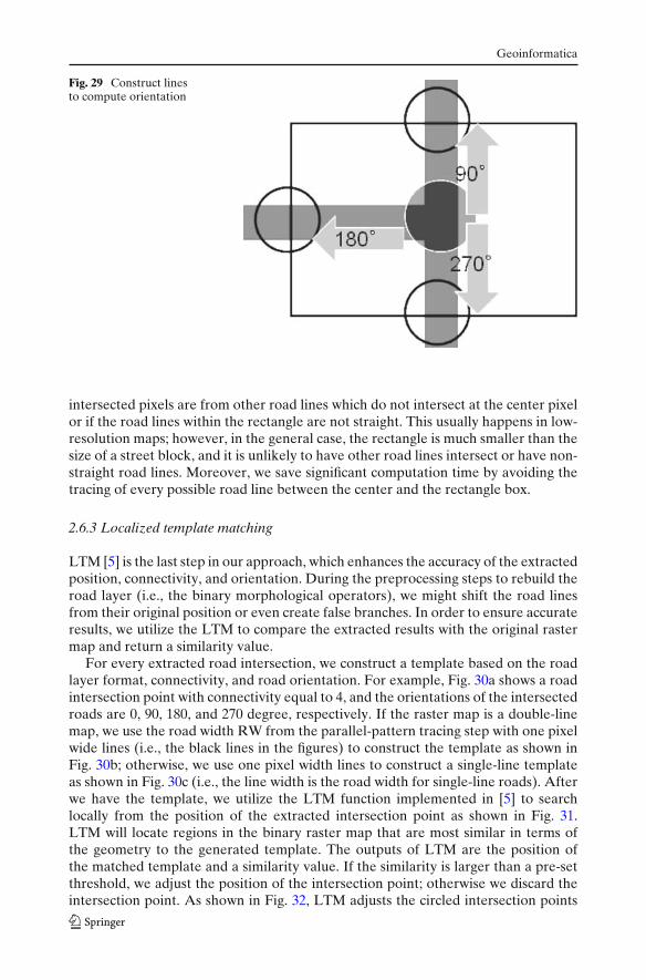
The connectivity of an interest point is the number of foreground pixels thatintersects with this rectangle since the road lines are all single pixel width. If theconnectivity is less than three, we discard the point; otherwise it is identified as aroad intersection point. Subsequently, we link the interest points to the intersectedforeground pixels on the rectangle boundaries to compute the slope (i.e., orientation)of the road lines as shown in Fig. 29.

In this step, we do not trace the pixels between the center pixel and the intersectedpixels at the rectangle boundaries. In general, this step could introduce errors if the

Fig. 28 The intersection candidates (gray circles) of a portion of the TIGER/Line Map. a The interestpoints. b Not an intersection. c An intersection

Geoinformatica

Fig. 29 Construct linesto compute orientation

intersected pixels are from other road lines which do not intersect at the center pixelor if the road lines within the rectangle are not straight. This usually happens in low-resolution maps; however, in the general case, the rectangle is much smaller than thesize of a street block, and it is unlikely to have other road lines intersect or have non-straight road lines. Moreover, we save significant computation time by avoiding thetracing of every possible road line between the center and the rectangle box.

2.6.3 Localized template matching

LTM [5] is the last step in our approach, which enhances the accuracy of the extractedposition, connectivity, and orientation. During the preprocessing steps to rebuild theroad layer (i.e., the binary morphological operators), we might shift the road linesfrom their original position or even create false branches. In order to ensure accurateresults, we utilize the LTM to compare the extracted results with the original rastermap and return a similarity value.

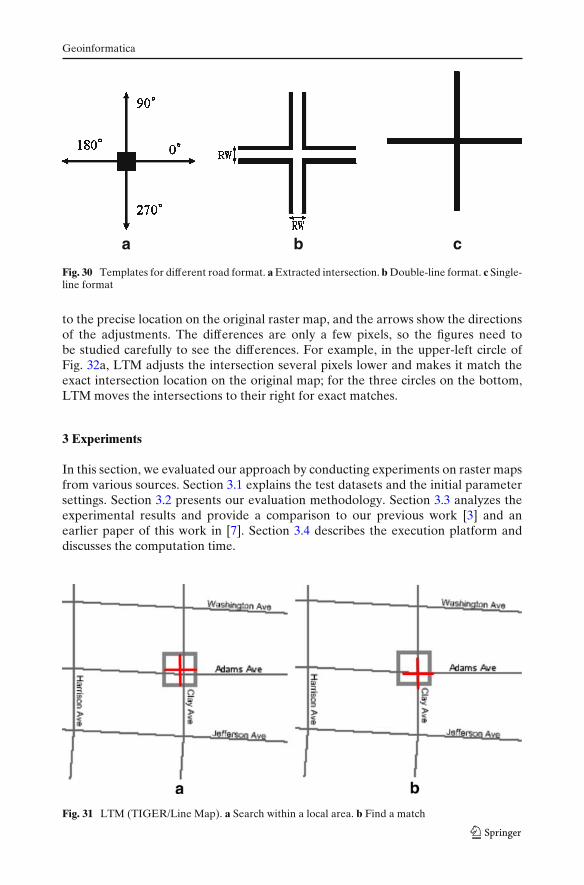
For every extracted road intersection, we construct a template based on the roadlayer format, connectivity, and road orientation. For example, Fig. 30a shows a roadintersection point with connectivity equal to 4, and the orientations of the intersectedroads are 0, 90, 180, and 270 degree, respectively. If the raster map is a double-linemap, we use the road width RW from the parallel-pattern tracing step with one pixelwide lines (i.e., the black lines in the figures) to construct the template as shown inFig. 30b; otherwise, we use one pixel width lines to construct a single-line templateas shown in Fig. 30c (i.e., the line width is the road width for single-line roads). Afterwe have the template, we utilize the LTM function implemented in [5] to searchlocally from the position of the extracted intersection point as shown in Fig. 31.LTM will locate regions in the binary raster map that are most similar in terms ofthe geometry to the generated template. The outputs of LTM are the position ofthe matched template and a similarity value. If the similarity is larger than a pre-setthreshold, we adjust the position of the intersection point; otherwise we discard theintersection point. As shown in Fig. 32, LTM adjusts the circled intersection points

Geoinformatica

a b c

Fig. 30 Templates for different road format. a Extracted intersection. b Double-line format. c Single-line format

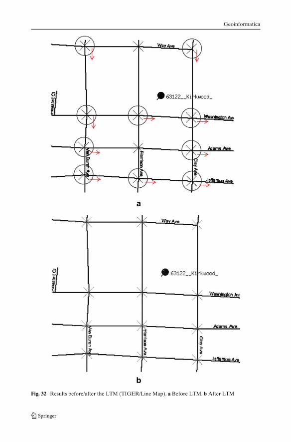
to the precise location on the original raster map, and the arrows show the directionsof the adjustments. The differences are only a few pixels, so the figures need tobe studied carefully to see the differences. For example, in the upper-left circle ofFig. 32a, LTM adjusts the intersection several pixels lower and makes it match theexact intersection location on the original map; for the three circles on the bottom,LTM moves the intersections to their right for exact matches.

3 Experiments

In this section, we evaluated our approach by conducting experiments on raster mapsfrom various sources. Section 3.1 explains the test datasets and the initial parametersettings. Section 3.2 presents our evaluation methodology. Section 3.3 analyzes theexperimental results and provide a comparison to our previous work [3] and anearlier paper of this work in [7]. Section 3.4 describes the execution platform anddiscusses the computation time.

Fig. 31 LTM (TIGER/Line Map). a Search within a local area. b Find a match

Geoinformatica

Fig. 32 Results before/after the LTM (TIGER/Line Map). a Before LTM. b After LTM

Geoinformatica

3.1 Experimental setup

We experimented with computer generated maps and scanned maps from 12 sources8

covering cities of the United States and some European countries. We first arbi-trarily selected 70 detailed street maps with a resolution range from 1.85 m/pixelto 7 m/pixel.9 In addition, we deliberately selected 7 low-resolution abstract maps(resolutions range from 7 m/pixel to 14.5 m/pixel) to test our approach on morecomplex raster maps that have significant overlap between lines and characters.

We did not use any prior information about the input maps. Instead we used aset of default parameters for all the input maps based on practical experience on asmall set of data (disjoint with our test dataset in this experiment), which may notproduce the best results for all raster map sources but demonstrate our capabilityto handle a variety of maps. The size of small connected objects to be removed inthe text/graphics separation step is set to 20-by-20 pixels. The number of iterationsfor the binary dilation and erosion operators on a single-line map are three andtwo respectively (i.e., a gap smaller than six pixels can be fixed). In the intersectionfiltering and connectivity and orientation extracting step, we used a 21-by-21 pixelrectangular box (10 pixels to the left, 10 pixels to the right plus one center pixel). Thesimilarity threshold for the LTM is 50%. We could optimize these parameters forone particular source to produce the best results if we incorporate prior knowledgeof the sources in advance.

3.2 Evaluation methodology

The output of our approach is a set of road intersection positions along with theroad connectivity and the orientations. We first report the precision (correctness)and recall (completeness)10 for the accuracy of the extracted intersection positions.For the displacement quality of the results, we randomly selected two maps fromeach source to examine the positional displacement. We also report the geometrysimilarity between the intersection templates we extracted and the original map toanalyze the quality of the road connectivity and orientation.

The precision (correctness) is defined as the number of correctly extracted roadintersection points divided by the number of extracted road intersection points.The recall (completeness) is defined as the number of correctly extracted roadintersection points divided by the number of road intersections on the raster map.The positional displacement is the distance in pixels between the correctly extractedroad intersection points and the corresponding actual road intersections. Correctlyextracted road intersection points are defined as follows: if we can find a roadintersection on the original raster map within a N pixel radius of the extractedroad intersection point, it is considered a correctly extracted road intersection point.Based on our practical experience, if an extracted intersection is within five pixelradius to any road intersections on the original map, it usually corresponds to

8ESRI Map, MapQuest Map, TIGER/Line Map, Yahoo Map, A9 Map, MSN Map, Google Map,Map24 Map, ViaMichelin Map, Multimap Map, USGS Topographic Map, Thomas Brothers Map.9Some of the sources do not provide resolution information.10The terms precision and recall are common evaluation terminologies in information retrieval andcorrectness and completeness are often used alternatively in geomatics and remote sensing [12].

Geoinformatica

an actual intersections on the original map but was shifted during the extraction;otherwise it is more likely a false-positive generated during our process to rebuildthe roads. Thus, N equal to five is used as the upper bound to report our results.We report the precision and recall as we vary N from 0 to 5 for a subset of testingdata in Section “3.3;” and we use N equal to 5 for any other places in the paperwhen precision and recall are mentioned. N represents the maximum positionaldisplacements an application can tolerate. Different usages of the extracted inter-sections have different tolerance levels on the value of N. For example, consider anapplication that utilizes the extracted intersections as seed templates to search forneighborhood road pixels on aerial imagery [13], it needs as many intersections aspossible; however, it is likely to have a lower requirement on the positional accuracyof the intersections (i.e., N can be larger). On the other hand, a conflation systemsuch as [5] requires higher positional accuracy (i.e., a smaller N) to match the setof road intersections to another set of road intersections from another source. Roadintersections on the original maps are defined as the intersection points of two ormore road lines for single-line maps or any pixel inside the intersection areas wheretwo or more roads intersect for double-line maps.

The geometric similarity represents the similarity between the extracted intersec-tion template and the binary raster map, which is computed with LTM as describedin Section 2.6.3 and used in [4]. For an intersection template T with w x h pixels andthe binary raster map B, the geometric similarity is defined in as:

GS(T) =∑h

y=1

∑wx=1 T(x, y)B(X + x, Y + y)

√∑hy=1

∑wx=1 T(x, y)2

∑hy=1

∑wx=1 B(X + x, Y + y)2

(1)

where T(x,y) equals one, if (x,y) belongs to the intersection template; otherwiseT(x,y) equals zero. B(x,y) equals one, if (x,y) is a foreground pixels on the binaryraster map; otherwise B(x,y) equals zero. In other words, the geometric similarity isa normalized cross correlation between the template and the binary raster map whichranges from zero to one [4].

3.3 Experimental results

We report the results with respect to the map sources as shown in Table 2. Theaverage precision is 95% and the recall is 75% under the set of parameters discussedin Section 3.1. In particular, for map sources like the A9 Map, the Map24 Map, andthe ViaMichelin Map, the precision is 100% because of the fine quality of their maps(i.e., less noise, same width roads etc.). In our experiments the USGS TopographicMaps have the lowest precision and recall besides the low-resolution raster maps.This is because USGS Topographic Maps contain more information layers thanother map sources and the quality of USGS Topographic Maps is not as good ascomputer generated raster maps due to the poor scan quality. The average geometricsimilarity of the extracted intersection template generated from LTM is 72%. Wecan improve the similarity if we track the line pixels when filtering the intersectionsto generate the templates, but it will require more computation time. Our approachgenerates a set of representative features for applications that require high quality ofcorresponding features for their matching process. In [5], a map to imagery conflationsystem proposed by Chen et al. build on the results of our approach (i.e., the set of

Geoinformatica

Table 2 Average precision, recall, and F-measure with respect to various sources

Map source (number of test maps) Precision (%) Recall (%) F-Measure (%)

ESRI map (10) 93 71 81MapQuest map (9) 98 66 79TIGER/Line map (9) 97 84 90Yahoo map (10) 95 76 84A9 map (5) 100 93 97MSN map (5) 97 88 92Google map (5) 98 86 91Map24 map (5) 100 82 90ViaMichelin map (5) 100 98 99Multimap map (5) 98 85 91USGS Topographic map (10) 82 60 69Thomas Brothers map (2) 98 65 79

road intersection templates) and achieved their goal to identify the geospatial extentof the raster map and to align the map with satellite imagery.

The value of positional displacements for two randomly selected maps from eachsource is 0.25 pixels on average; and the Root Mean Squared Error (RMSE) is 0.82,which means the majority of extracted intersections are within one pixel radius ofthe actual intersections on the map. Some extracted intersections are still not on theprecise original position since we construct the LTM template using 1-pixel widthroads instead of using the original road line width, which is unknown. As shown inFig. 33, we also report the recall and precision with the positional displacement, N,varies from 0 pixels (i.e., we extract the exact position) to 5 pixels. Intuitively, theprecision and recall are higher when the N increases. For applications that do not

95% 96% 97%

74%76%

80%82% 83% 84%86%

88%

93%

65%

71%67%

74%73%73%

0%

10%

20%

30%

40%

50%

60%

70%

80%

90%

100%

0 pixel 1 pixel 2 pixels 3 pixels 4 pixels 5 pixels

Precision

Recall

F-Measure

Fig. 33 The precision and recall with respect to the positional displacement

Geoinformatica

Table 3 Experimental results with respect to the resolution

Precision (%) Recall (%)

Resolution higher then 7 m/pixel (70 maps) 95 75Resolution lower then 7 m/pixel (7 maps) 83 27

require finding the exact location of the intersections, we can achieve higher precisionand recalls.

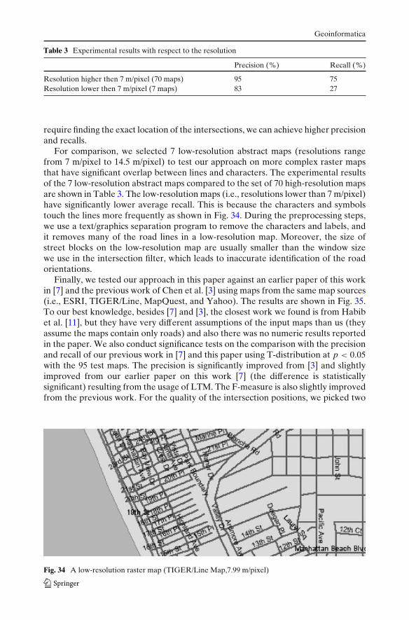
For comparison, we selected 7 low-resolution abstract maps (resolutions rangefrom 7 m/pixel to 14.5 m/pixel) to test our approach on more complex raster mapsthat have significant overlap between lines and characters. The experimental resultsof the 7 low-resolution abstract maps compared to the set of 70 high-resolution mapsare shown in Table 3. The low-resolution maps (i.e., resolutions lower than 7 m/pixel)have significantly lower average recall. This is because the characters and symbolstouch the lines more frequently as shown in Fig. 34. During the preprocessing steps,we use a text/graphics separation program to remove the characters and labels, andit removes many of the road lines in a low-resolution map. Moreover, the size ofstreet blocks on the low-resolution map are usually smaller than the window sizewe use in the intersection filter, which leads to inaccurate identification of the roadorientations.

Finally, we tested our approach in this paper against an earlier paper of this workin [7] and the previous work of Chen et al. [3] using maps from the same map sources(i.e., ESRI, TIGER/Line, MapQuest, and Yahoo). The results are shown in Fig. 35.To our best knowledge, besides [7] and [3], the closest work we found is from Habibet al. [11], but they have very different assumptions of the input maps than us (theyassume the maps contain only roads) and also there was no numeric results reportedin the paper. We also conduct significance tests on the comparison with the precisionand recall of our previous work in [7] and this paper using T-distribution at p < 0.05with the 95 test maps. The precision is significantly improved from [3] and slightlyimproved from our earlier paper on this work [7] (the difference is statisticallysignificant) resulting from the usage of LTM. The F-measure is also slightly improvedfrom the previous work. For the quality of the intersection positions, we picked two

Fig. 34 A low-resolution raster map (TIGER/Line Map,7.99 m/pixel)

Geoinformatica

Fig. 35 Comparison withprevious work

83% 84%

76%

94%96%

N/A

74%74%

N/A0%

10%

20%

30%

40%

50%

60%

70%

80%

90%

100%

Chen et al. 04 ACM-GIS'05 paper on

this work

This paper

PrecisionRecallF-Measure

maps for each source to calculate the positional displacement. The RMSE of thepositional displacement using the approach in this paper is 1.01, which is improvedfrom 1.37 in [7] due to the use of LTM. The recall in [7] is slightly higher than therecall of this paper (the difference is not statistically significant) since the LTM filterssome correct intersections with incorrect orientation and connectivity templates.Two example results from our experiments are shown in Fig. 36. In these figures,an “X” marks the one road intersection point extracted by our system.

3.4 Computation time

Our test platform is an Intel Xeon 1.8 GHz Dual Processors server with 1 GBmemory and the development tool is Microsoft Visual Studio 2003. The efficiency

Fig. 36 Road intersectionextraction. a TIGER/Line map. b USGS Topographic map

Geoinformatica

0 sec

20 sec

40 sec

60 sec

80 sec

100 sec

120 sec

0 pixels 20,000

pixels

40,000

pixels

60,000

pixels

80,000

pixels

100,000

pixels

120,000

pixels

140,000

pixels

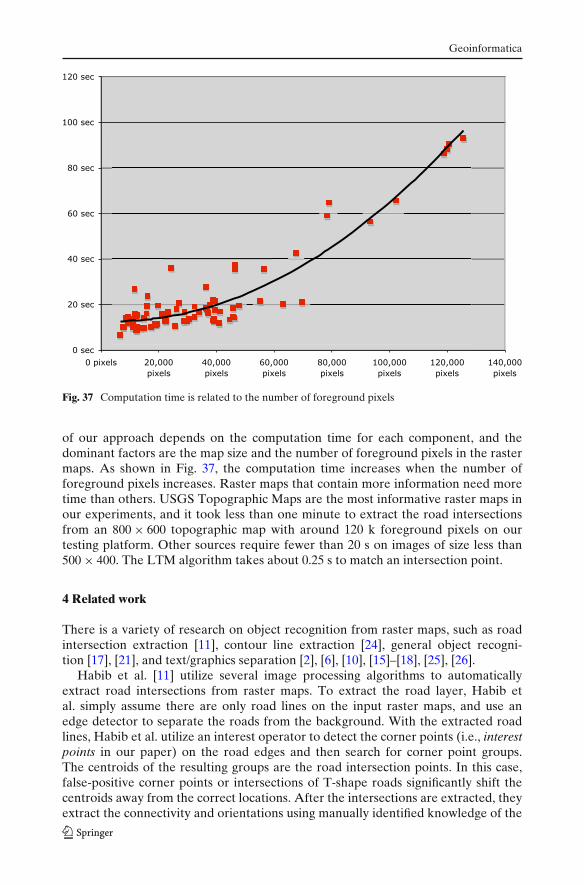
Fig. 37 Computation time is related to the number of foreground pixels

of our approach depends on the computation time for each component, and thedominant factors are the map size and the number of foreground pixels in the rastermaps. As shown in Fig. 37, the computation time increases when the number offoreground pixels increases. Raster maps that contain more information need moretime than others. USGS Topographic Maps are the most informative raster maps inour experiments, and it took less than one minute to extract the road intersectionsfrom an 800 × 600 topographic map with around 120 k foreground pixels on ourtesting platform. Other sources require fewer than 20 s on images of size less than500 × 400. The LTM algorithm takes about 0.25 s to match an intersection point.

4 Related work

There is a variety of research on object recognition from raster maps, such as roadintersection extraction [11], contour line extraction [24], general object recogni-tion [17], [21], and text/graphics separation [2], [6], [10], [15]–[18], [25], [26].

Habib et al. [11] utilize several image processing algorithms to automaticallyextract road intersections from raster maps. To extract the road layer, Habib etal. simply assume there are only road lines on the input raster maps, and use anedge detector to separate the roads from the background. With the extracted roadlines, Habib et al. utilize an interest operator to detect the corner points (i.e., interestpoints in our paper) on the road edges and then search for corner point groups.The centroids of the resulting groups are the road intersection points. In this case,false-positive corner points or intersections of T-shape roads significantly shift thecentroids away from the correct locations. After the intersections are extracted, theyextract the connectivity and orientations using manually identified knowledge of the

Geoinformatica

road format and the road width. In comparison, our approach detects the road layerformat and road width automatically to rebuild the road layer. Moreover, the usageof LTM with the road width ensures the extracted intersections are on the originalpositions without manually verifying the results.

Salvatore and Guitton [24] use a color classification technique to extract contourlines from the topographic maps. Their technique requires prior knowledge togenerate a proper set of color thresholds for a specific set of maps. However,in reality, the thresholds for different topographic maps covering different areasmay vary depending on the quality of the raster map. With our approach, weseparate the contour lines from the roads by distinguishing their different geometricrepresentations. In addition, the previous work has the goal to ensure the resultingcontour lines have continuity similar to the original while our focus is on the roadlines that are close to the intersections.

Samet et al. [21] use the legends in a learning process to identify objects on theraster maps. Meyers et al. [17] use a verification based approach with map legendsand specifications to extract data from raster maps. These approaches both needprior knowledge (i.e., legend layer and map specification) of the input raster maps,and the training process needs to be repeated when the map source changes.

Finally, much research work has been performed in the field of text/graphicsseparation from documents and maps [2], [6], [10], [15]–[18], [25], [26], which isrelated to one of our step to extract and rebuild the road layer. Among the text/graphics separation research, [2], [10], [26] assume that the line and characterpixels are not overlapping and they extract characters by tracing and groupingconnected objects. Cao et al. [6] detects characters from more complex documents(i.e., characters overlap lines) using the differences of the length of line segments incharacters and lines. Li et al. [15, 16] and Nagy et al. [18] first separate the charactersfrom the lines using connected component analysis and then focus on local area torebuild the lines and characters using various methods. Generally, the text/graphicsseparation research emphasize on extracting characters, hence it provides a partialsolution to our goal to extract the intersection templates. In Section 2.2.2, we describehow we incorporate the algorithm from [6] to remove the characters before we utilizethe binary morphological operators to rebuild the roads.

The main difference between our approach and the previous work on mapproblems is that the previous work requires additional information hence theyprovide partial solutions to the problem of automatic road intersection extraction.We assume a more general scenario to handle various map sources [9]; and ourapproach requires no prior knowledge while it still can be tuned with additionalinformation, if available.

5 Conclusion and future work

The main contribution of this paper is to provide a complete framework to automati-cally and accurately extract the intersections from raster maps. We also identify othervaluable information such as the road format (i.e., single-line format or double-lineformat) and road width to help the extraction process.

Our approach achieves 95% precision and 75% recall on average when auto-matically extracting road intersections from raster maps with resolution higher than

Geoinformatica

7m/pixel without any prior information. The result is a set of accurate features thatcan be used to exploit other geospatial data or to intergrate a raster map with othergeospatial sources, thus creating an integrated view. For example, in [5], Chen et al.used the extracted intersections to align the maps to imagery. Moreover, for aroad extraction application, the georeferenced road intersections can be used asseed templates to extract the roads from imagery [13]. In the work in [9], Desaiet al. applied our automatic intersection extraction technique on maps returnedfrom image search engines and successfully identify the road intersection points forgeospatial fusion systems to identify the geocoordinates of the input maps.

There are three primary assumptions of our current approach. First, the back-ground pixels must be separable using the difference in luminosity level from theforeground pixels. This means that the background pixels must have the dominantcolor in the raster maps. On certain raster maps that contain numerous objectsand the number of foreground pixels is larger than that of the background pixels,those foreground objects seriously overlap with each other making the automaticprocessing nearly impossible. Even if we can remove the background pixels onthese raster maps, removing noisy objects touching road lines results in too manybroken road segments that are difficult to reconnect. Second, although our approachworks with no prior knowledge of the map scales, low-resolution raster maps (i.e.,in our experiments, above 7 m/pixel) may result in low precision and recall. Third,as mentioned in Section 2.2.2, if the characters on the input map are significantlydifferent than our preset value, we cannot remove the character from lines and theresults will have many incorrectly identified intersections.

In future work, we plan to address these issues. First, we plan to exploit textureclassification methods [20] to handle those raster maps in which the background coloris not the dominate color such as tourist maps. Second, although the text/graphicsseparation program performs well with one set of default parameters in our exper-iments, we still need to specify these parameters for each map to achieve the bestresults. Instead of tuning for every map, we want to utilize classification methodsin the frequency domain [8], [14] to separate line and character textures, whichdo not require any geometric parameters. Third, we want to further enhance theextracted road layer. In our approach, we do not focus on repairing the road network,but rather on rebuilding the roads close to the intersections. Hence we generatea comparatively coarse road layer from the original raster map. With the help ofvectorization algorithms, we can further repair the road layer and generate the roadvector data from the raster maps.

Acknowledgements This research is based upon work supported in part by the United States AirForce under contract number FA9550-08-C-0010, in part by the National Science Foundation underAward No. IIS-0324955, in part by the Air Force Office of Scientific Research under grant numberFA9550-07-1-0416, in part by a gift from Microsoft, and in part by the Department of HomelandSecurity under ONR grant number N00014-07-1-0149. The U.S. Government is authorized to repro-duce and distribute reports for Governmental purposes notwithstanding any copyright annotationthereon. The views and conclusions contained herein are those of the authors and should not beinterpreted as necessarily representing the official policies or endorsements, either expressed orimplied, of any of the above organizations or any person connected with them. We would like tothank Dr. Chew Lim Tan for his generous sharing of their code in [6].

Geoinformatica

References

1. Agam G, Dinstein I (1996) Generalized morphological operators applied to map-analysis. In:The proceedings of the 6th international workshop on advances in structural and syntacticalpattern recognition. Springer-Verlag, pp 60–69

2. Bixler JP (2000) Tracking text in mixed-mode documents. In: The ACM conference on documentprocessing systems, ACM, Santa Fe, New Mexico, pp 177–185

3. Chen C-C, Knoblock CA, Shahabi C, Chiang Y-Y, Thakkar S (2004) Automatically and accu-rately conflating orthoimagery and street maps. In: The 12th ACM international symposium onadvances in geographic information systems, ACM, Washington, D.C., pp 47–56

4. Chen C-C, Knoblock CA, Shahabi C (2006) Automatically conflating road vector data withorthoimagery. Geoinformatica 10(4):495–530

5. Chen C-C, Knoblock CA, Shahabi C (2008) Automatically and accurately conflating raster mapswith orthoimagery. GeoInformatica (in press)

6. Cao R, Tan CL (2001) Text/graphics separation in maps. In: The 4th international work-shop on graphics recognition algorithms and applications, Kingston, Ontario. Springer Verlag,pp 167–177

7. Chiang Y-Y, Knoblock CA, Chen C-C (2005) Automatic extraction of road intersections fromraster maps. In: The 13th ACM international symposium on advances in geographic informationsystems, Bremen, ACM

8. Chiang Y-Y, Knoblock CA (2006) Classification of line and character pixels on raster maps usingdiscrete cosine transformation coefficients and support vector machines. In: The internationalconference on pattern recognition, Hong Kong, IEEE Computer Society

9. Desai S, Knoblock CA, Chiang Y-Y, Desai K, Chen C-C (2005) Automatically identifying andgeoreferencing street maps on the web. In: The 2nd international workshop on geographicinformation retrieval, Bremen, ACM

10. Fletcher LA, Kasturi R (1988) A robust algorithm for text string separation from mixedtext/graphics images. IEEE Trans Pattern Anal Mach Intell 10(6):910–918

11. Habib AF, Uebbing RE (1999) Automatic extraction of primitives for conflation of raster maps.Technical report. The Center for Mapping, The Ohio State University

12. Heipk C, May H, Wiedemann C, Jamet O. (1997) Evaluation of automatic road extraction. In:The ISPRS Conference, vol 32, pp 3–2W3

13. Koutaki G, Uchimura K (2004) Automatic road extraction based on cross detection in suburb.In: Image processing: algorithms and systems III. Proceedings of the SPIE, vol 5299, pp 337–344

14. Keslassy I, Kalman M, Wang D, Girod B (2001) Classification of compound images based ontransform coefficient likelihood. In: The international conference on image processing, Thessa-loniki, IEEE

15. Li L, Nagy G, Samal A, Seth S, Xu Y (1999) Cooperative text and line-art extraction from atopographic map. In: Proceedings of the 5th international conference on document analysis andrecognition, IEEE

16. Li L, Nagy G, Samal A, Seth S, Xu Y (2000) Integrated text and line-art extraction from atopographic map. IJDAR 2(4):177–185

17. Myers GK, Mulgaonkar PG, Chen C-H, DeCurtins JL, Chen E (1996) Verification-based ap-proach for automated text and feature extraction from raster-scanned maps. In: Lecture notes incomputer science, vol 1072. Springer, pp 190–203

18. Nagy G, Sama A, Set S, Fisher T, Guthmann E, Kalafala K, Li L, Sivasubraniam S, Xu Y (1997)Reading street names from maps - Technical challenges. In: Procs. GIS/LIS conference, pp 89–97

19. Pratt WK (2001) Digital image processing: PIKS inside, 3rd edn. Wiley-Interscience, New York20. Randen T, Husoy JH (1999) Filtering for texture classification: a comparative study. IEEE Trans

Pattern Anal Mach Intell 21(4):291–31021. Samet H, Soffer A (1994) A legend-driven geographic symbol recognition system. In: The 12th

international conference on pattern recognition, IEEE, Jerusalem, vol 2, pp 350–355, October22. Shi J, Tomasi C (1994) Good features to track. In: The IEEE conference on computer vision and

pattern recognition, IEEE, Seattle23. Sezgin M, Sankur B (2004) Survey over image thresholding techniques and quantitative perfor-

mance evaluation. J Electron Imaging 13(1):146–16524. Salvatore S, Guitton P (2001) Contour line recognition from scanned topographic maps. Techni-

cal report. University of Erlangen

Geoinformatica

25. Tang YY, Lee S-W, Suen CY (1996) Automatic document processing: a survey. Pattern Recogn29(12):1931–1952

26. Velázquez A, Levachkine S (2003) Text/graphics separation and recognition in raster-scannedcolor cartographic maps. In: The 5th international workshop on graphics recognition algorithmsand applications, Barcelona, Catalonia

27. Zack GW, Rogers WE, Latt SA (1977) Automatic measurement of sister chromatid exchangefrequency. J Histochem Cytochem 25(7):741–753

Yao-Yi Chiang is currently a Ph.D. student at the University of Southern California (USC). Hereceived his B.S. in Information Management from National Taiwan University in 2000 and then hisM.S. degree in Computer Science from the USC in December 2004. His research interests are on theautomatic fusion of geographical data. He has worked extensively on the problem of automaticallyutilize raster maps for understanding other geospatial sources and has wrote and co-authored severalpapers on automatically fusing map and imagery as well as automatic map processing. Prior to hisdoctoral study at USC, Yao-Yi worked as a Research Scientist for Information Sciences Institute andGeosemble Technologies.

Craig A. Knoblock is a Senior Project Leader at the Information Sciences Institute and a ResearchProfessor in Computer Science at the USC. He is also the Chief Scientist for Geosemble Tech-nologies, which is a USC spinoff company that is commercializing work on geospatial integration.He received his Ph.D. in Computer Science from Carnegie Mellon. His current research interestsinclude information integration, automated planning, machine learning, and constraint reasoningand the application of these techniques to geospatial data integration. He is a Fellow of the AmericanAssociation of Artificial Intelligence.

Geoinformatica

Cyrus Shahabi is currently an Associate Professor and the Director of the Information Laboratory(InfoLAB) at the Computer Science Department and also a Research Area Director at the NSF’sIntegrated Media Systems Center at the USC. He received his B.S. in Computer Engineering fromSharif University of Technology in 1989 and then his M.S. and Ph.D. degrees in Computer Sciencefrom the USC in May 1993 and August 1996, respectively. He has two books and more than hundredarticles, book chapters, and conference papers in the areas of databases, geographic informationsystem (GIS) and multimedia. Dr. Shahabi’s current research interests include Geospatial andMultidimensional Data Analysis, Peer-to-Peer Systems and Streaming Architectures. He is currentlyan associate editor of the IEEE Transactions on Parallel and Distributed Systems and on theeditorial board of ACM Computers in Entertainment magazine. He is also a member of the steeringcommittees of IEEE NetDB and the general co-chair of ACM GIS 2007. He serves on manyconference program committees such as VLDB 2008, ACM SIGKDD 2006 to 2008, IEEE ICDE2006 and 2008, SSTD 2005 and ACM SIGMOD 2004. Dr. Shahabi is the recipient of the 2002National Science Foundation CAREER Award and 2003 Presidential Early Career Awards forScientists and Engineers. In 2001, he also received an award from the Okawa Foundations.

Ching-Chien Chen is the Director of Research and Development at Geosemble Technologies. Hereceived his Ph.D. degree in Computer Science from the USC for a dissertation that presented novelapproaches to automatically align road vector data, street maps and orthoimagery. His researchinterests are on the fusion of geographical data, such as imagery, vector data and raster maps withopen source data. His current research activities include the automatic conflation of geospatial data,automatic processing of raster maps and design of GML-enabled and GIS-related web services.Dr. Chen has a number of publications on the topic of automatic conflation of geospatial data sources.