Saitou, K., Jakiela, M. J., “Automated Optimal Design of Mechanical ConformationalSwitches,” Artificial Life 2(2):129–156, 1995.

Automated Optimal Design of Mechanical

Conformational Switches

Kazuhiro Saitou Mark J. Jakiela ∗

Computer-Aided Design LaboratoryMassachusetts Institute of Technology

Abstract

Bacteriophage viruses spontaneously self-assemble in the presence of their component parts (cer-tain protein molecules). It is believed that conformational switches, interacting chemical bondingsites that allow tentative incorrect bonds, facilitate this randomized assembly process. A one-dimensional conformational switch is proposed and used to study the randomized assembly of me-chanical parts. A genetic algorithm is used to search the space of parameterized switch designs tomaximize the rate of a desired assembly.

Keywords: randomized assembly, mechanical conformational switches, genetic optimization

1 Introduction

1.1 Viruses and conformational switching

Viruses are one of the simplest known life forms. An interesting characteristic of some viruses is that theycan spontaneously self-assemble [1]. If the correct components (various proteins molecules) of a virus arebrought into proximity, chemical bonds will form in appropriate locations to create the virus structure.The organism arises, therefore, from disorganized numbers of its components in its environment.

Over the past several years, Thompson, Goel, and associated researchers have developed and docu-mented a computer model that simulates the assembly and operation of a particular type of virus, the T4bacteriophage [11, 12, 3]. A simulation builds a simplified model of a virus from building blocks which areabstractions of the protein molecules. These building blocks bond to one another at prespecified bondsites with prespecified bond strengths. As molecular bonding is a thermodynamic process, the bondingamong building blocks, and hence the simulation, is governed by the minimization of free energy in thesystem. With an appropriately designed (various sizes and aspect ratios, bond site locations on eachbuilding block, and bond strengths) set of building blocks, Thompson and Goel have developed two- [11]and three- [12] dimensional augmented cellular automata models of viral assembly and operation.

A key aspect of the simulation scheme is the concept of conformational switching. If a building blockhas several bond sites, a conformational switch causes the bond at one site to influence a bond at anothersite. A bond made at one site can weaken or strengthen the bond potential at another site, or a bondat one site may destroy the bond at another site, in the manner of a latch.

Figure 1 shows an example of such conformational switching in the inhibition of protein enzymes byspecific end-product inhibitor molecules. The catalytic activity of many protein enzymes are activatedby binding their substrates, and forming enzyme-substrate complexes (Figure 1-a). The end-productinhibitor blocks the enzyme activity by reversibly binding to the enzyme at a site other than the activesite (the region that binds the substrates). The binding of the inhibitor causes a conformational changeat the active site on the enzyme, which prevents the enzyme from combining with its substrate (Figure 1-b). The chemical forces binding a specific end-product inhibitor to an enzyme are weak secondary forcessuch as hydrogen bonds, salt linkages, and van der Waals forces and do not involve covalent bonding.Hence, inhibition can be quickly reversed once the end-product concentration is reduced to a low level.

∗Author to whom correspondence should be addressed: Massachusetts Institute of Technology, Department of Me-chanical Engineering, 77 Massachusetts Avenue, Room 3-461a, Cambridge, MA 02139; Phone: (617) 253-6552; FAX:(617)258-9346; email: {jakiela, kazu}@mit.edu.

1

Artificial Life 2(2):129–156, 1995. 2

( a )

enzyme substrate enzyme-substrate complex

( b )

enzyme substrate inactive enzymeend-product inhibitor

conformational change

Figure 1: A biological example of conformational switching: inhibition of protein enzymes by specificend-product inhibitor molecules (abstracted from Figure 4-21 of [13])

In the simulation of the viral assembly, conformational switches allow the tentative assembly ofsubunits that may not be assembled together in the final complete correct virus. In the work of Thompsonand Goel, the conformational switches are simply predetermined numerical relationships. We note, incontrast, the work of Penrose [9], who suggests several designs for mechanical conformational switchesthat are used in devices that self-reproduce. These conformational switches are binary, in the sense thata bond at one location breaks a bond existing at another location or prevents a bond from occurring atanother location. The self-reproducing devices attach to some number of other “neutral” sub-devices.When the correct number and arrangement of sub-devices are linked, conformational switches cause theentire chain to cleave into two copies of the original self-reproducing device in a process akin to celldivision.

Our interest in this paper is the design of such mechanical conformational switches. In particular,we will describe the optimization of a specific parameterized mechanical conformational switch design.The objective of this optimization is to maximize the assembly rate of a set of parts held together withthese conformational switches. The assembly process considered is a randomized juxtaposition of theparts which is loosely similar to the randomized interaction of bacteriophage components prior to theviral assembly. We will first describe the switch design and how it functions. Then we will describe howthe design is parameterized and how it can be represented with a genetic algorithm chromosome. Anevolutionary (genetic) algorithm is used to search the space of possible switch designs to maximize therate of a desired assembly. Several examples are presented and discussed. Before proceeding to theseissues, however, we discuss potential practical uses for mechanical conformational switches and previouswork in the area.

1.2 Practical applications of conformational switching

In the biological assembly of bacteriophage viruses, conformational switches are important in allowingthe assembly of randomly arranged and randomly moving components. We will refer to this as a ran-domized assembly process. Similarly, in domains other than the biological, we feel that conformationalswitches will be important in any type of randomized assembly process. Practical applications of con-formational switches will follow from practical applications of randomized assembly. What are somepractical applications of randomized assembly?

• Assembly at very high rates. The common image of assembly is a robotic or human handgrasping one part at a time, assembling it into a product held on a fixture. There are naturallimits to the speed with which this process can be carried out. Adding more human or robot handsis often not cost effective to achieve very high rates of assembly. Working in the domain of highvolume assembly of consumer electromechanical products (cameras, videocassette recorders, etc.),

Artificial Life 2(2):129–156, 1995. 3

we developed the concept of mass aggregate assembly [8, 7]. This process employs part presenta-tion devices (feeding and orienting machines) that transport bulk quantities of parts to actuallyassemble large quantities of parts in parallel simultaneously. In the implementation developed byMoncevicz [6], parts are “palletized” by using vibration to convey them over a plastic “pallet”into which are carved an array of relief shapes that trap and orient the flowing parts. To achieveparallel assembly of two parts, a quantity of the first part is palletized. This first part is designedsuch that once held in the pallet relief forms, it becomes integral with the pallet for the purposeof palletizing a quantity of the second part. The second part palletization actually assembles aquantity of the second part to the first part. The mated part pair is removed as a subassemblyunit from the pallet. Since many part insertions occur simultaneously, a very high assembly ratecan be achieved.

We believe that this layered palletization process (and other similar processes) could be employed inmore cases if temporary nonfunctional shape features could be added to the pallet or the palletizedparts. Between part layers, for example, a “primer layer” of nonfunctional “pseudo parts” couldbe palletized. The sole purpose of this primer layer would be to cause geometric shapes that wouldfacilitate the subsequent palletization of the next part layer. If the pseudo parts are not neededfor (or worse prevented) the functioning of the assembled device, they must be removed before thedevice is used. This could be accomplished if their design involved the use of a conformationalswitch that detached them upon the arrival and assembly of the part whose assembly they wereintended to facilitate.

• Assembly of very small things. Another problem with the common “part grasping” image ofassembly is that some parts are simply too small to grasp. A randomized process might be theonly possible approach. Yeh and Smith [14] used a (non-layered) palletization technique similarto [8, 7], to assemble microstructures. They fabricated trapezoidal galium arsenite (GaAs) blocksand a Si wafer with trapezoidal holes. Assembly is then done by releasing the GaAs blocks in acarrier fluid (ethanol) and dispensing the fluid over the Si wafer. Cohn et al. [2] experimentedwith the self-assembly of a small hexagonal lattice (1 mm in diameter) by placing a quantityof them on a slightly concave diaphragm that was agitated with a loudspeaker. Incorporatingconformational switching to such micro-scale randomized assembly processes might facilitate thenon-trivial assembly of very small parts.

• Assembly very far away. Consider trying to remotely assemble a set of components that are veryfar away. An example might be the construction of housing units on a distant planet. Teleoperationcontrol issues arise along with the problem of the cost of transmitting control signals back andforth to the remote site. An alternate approach might be to send quantities of the componentparts to the site, and outfit them with an autonomous means of locomotion. The parts could roamaround until they find each other and correctly assemble. Again, the similarities with the viralassembly process are clear, and conformational switches could be similarly useful.

1.3 Previous work

All three practical applications just described would require the optimization of the assembly rateachieved with the parts that could conformationally assemble. This is to say, for example, that thebest design of remote planet housing is the one that will assemble most quickly in the randomized as-sembly process. The objective of the design optimization for parts and related conformational switchesis therefore the maximization of assembly rate. This is the approach we have taken in this work.

In this context, the work most closely related to our efforts is that of Hosokawa et al. [5]. Theypropose a chemical kinetics analogy to randomized assembly. Chemical reactions are analogous to theassembly and/or disassembly of certain subsets of parts. The amount of each intermediate subassemblyis predicted given the initial quantities of each part and a relation describing the reaction dynamics. Aphysical experiment was devised by using a quantity of triangular parts that were fitted with conforma-tional switches made from movable magnets. These parts were assembled in a rotating box randomizer.Empirical results agreed reasonably well with predicted values. The important distinction with our work

Artificial Life 2(2):129–156, 1995. 4

( b )

bonding site( a )

conformational

change

Figure 2: one-dimensional conformational switch

1 1

bond site

bond configuration +1 -1 0

Figure 3: bond configurations

is that they do not address the design optimization of the part and switch design. Their emphasis is onverifying the chemical kinetics analogy.

2 Conformational switch model

2.1 One-dimensional conformational switch

Our design of a conformational switch for one-dimensional assembly is motivated by the “countingdevice” appearing in [9]. We extended this counting device model so that a part can form and destroya bond with another part.

As shown in Figure 2-a, a part has two bonding sites and a conformational switch is realized witha sliding bar mechanism that connects the two bonding sites. Conformational change is triggered byinteraction with another part (see Figure 2-b). Note that parts can be assembled in only one direction,say horizontally. In Figure 2, therefore, one can place a part on the left or the right of another part, butnot on the top or bottom. However, the model could easily be extended to the two-dimensional case.

A bond configuration is a variable which describes the shape of a bonding site. It takes a positivevalue if the corresponding site has convex shape, a negative value if the site is concave, and zero if thesite is flat. Examples of bond configurations and the corresponding shape of bonding sites are shown inFigure 3.

Artificial Life 2(2):129–156, 1995. 5

( b ) : unstable bond ==> conformational change

a + b = 1

( a ) : stable bonda + b <= 0

( c ) : no bond a + b > 1

Figure 4: three types of bonding

When bonding sites of two parts meet, they form either 1) a stable bond, 2) an unstable bond, or 3)no bond. The occurrences of these cases depend on the shape of the two bonding sites, or equivalently,the bond configurations of the sites. Let a and b be bond configurations of two bonding sites contactingeach other. These sites form a stable bond if a + b ≤ 0 (complementary), form an unstable bond ifa + b = 1 (fairly complementary), and form no bond if a + b > 1 (not complementary). Figure 4 showsexamples of each of the three cases.

An unstable bond induces conformational change of the involved bonding sites, which can propagateover the connected parts via the sliding bar mechanism. After the conformational changes, a stablebond is formed if a + b ≤ 0 and no bond is formed if a + b ≥ 1. Also, an existing bond is destroyedif a + b ≥ 1 after the conformational changes, which results in detaching of the corresponding parts.Figure 5 illustrates an example of such propagation and detaching.

Ambiguous situations may arise when conformational change can propagate in both directions or inno direction, such as the cases shown in Figure 6-a. To resolve such ambiguity, we assume an upstream

Figure 5: propagation of conformational changes and detaching

Artificial Life 2(2):129–156, 1995. 6

( a ) ambiguous situations

( b ) results by upstream propagation

??

upstream

upstream

downstream

Figure 6: priority to upstream propagation

propagation priority. As shown in Figure 6-b, conformational change propagates downstream (as definedin Figure 6), only when the upstream direction has a rigid end and downstream has a free end (thebottom picture of Figure 6-b). Otherwise, propagation goes upstream (the top and middle picture ofFigure 6-b).

2.2 One-dimensional randomized assembly

In the computer implementation of one-dimensional randomized assembly, we assumed that the processis sequential. In other words, one pairwise mating of two parts (possibly subassemblies of parts) occursat a given time. Given this assumption, a randomized assembly can be achieved in a straightforwardway by using a robot bin-picking metaphor described as follows:

Assume a random assortment of parts in a (one-dimensional) bin (Figure 7-a).

Step 1: The robot arm #1 randomly picks up a part from the bin. Then, robot arm #2 randomlypicks up another part from the bin (Figure 7-b).

Step 2: The two parts are pushed against each other, possibly causing formation and destruction ofbonds (Figure 7-c).

Step 3: The parts are randomly returned to the bin (Figure 7-d), possibly as an assembly.

The steps 1-3 are repeated until pre-specified conditions are satisfied (e.g. repeat for a specifiednumber of iterations, repeat until the number of parts decreases below a limit, etc.). It is assumed thatthe parts do not change their orientations, so in general, AB and BA are two distinct assemblies.

Artificial Life 2(2):129–156, 1995. 7

( a )

( c )

( d )

( b )

arm #1 arm #2

Figure 7: robot bin-picking metaphor

Artificial Life 2(2):129–156, 1995. 8

3 Genetic algorithm optimization

3.1 Genetic algorithms

Genetic algorithms (GAs) are an optimization technique in which points in the design space are analogousto organisms subject to a process of natural selection, or “survival of the fittest” [4]. The quality ofa design (or a point in the design space) is measured by a fitness function, which takes as input anencoded representation of the point, or a genetic “chromosome” of the design. GAs model reproduction inpopulations of such chromosomes over generations. In a given generation, designs with higher fitness havea higher probability to be selected for reproduction. During reproduction, two “parent” chromosomesare mated through genetic crossover, which results in two offspring chromosomes. Many generations ofsuch selection and mating will produce a highly-fit population of chromosomes, i.e. better designs.

3.2 Formulation of GA search

We are interested in designing conformational switches that, when randomly assembled, maximize therate of a desired assembly. More precisely, the problem is stated as follows:

Given: the total number of parts, and the number of each kind of part in the bin (in other words, theinitial state of the bin)

Find: the optimal design of conformational switches that maximizes the assembly rate (i.e. yield) of adesired set of parts in the process of randomized assembly.

Note that we are designing not only the bar mechanisms, but also the initial bond configurations.The above problem is formulated by parameterizing the design of the conformational switches, withgenetic algorithms used to search the parameter space of possible switch designs.

The one-dimensional conformational switch of a part is uniquely specified in terms of four parameters:left config, right config, link, and bar length. Left config and right config are the initial bond configura-tions of the left bond site and the right bond site, respectively. Link is a Boolean variable that specifiesthe existence of the conformational link (a bar mechanism) in a part. If link is TRUE, there is a confor-mational link between the two bond sites, so they can undergo conformational change. If link is FALSE,there is no conformational link, so the bond configurations do not change from their initial values (i.e. asolid part). Bar length is an upper limit on right config and left config. In order for a design to be valid,we need left config, right config ≤ bar length. Note that if left config = right config = bar length,the bar cannot move at all. Also, bar length is ignored if link is FALSE.

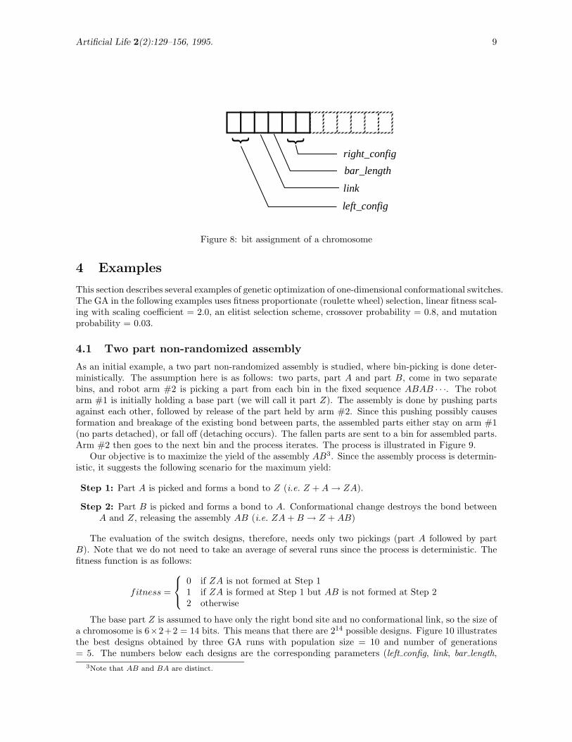
A chromosome used in genetic search is a binary string that encodes the above design parametersfor all kinds of parts in the bin. For the examples in the next section (unless otherwise stated), two bitsare assigned for each of left config and right config, and one bit for link and bar length1. The location ofthese bits on a chromosome is shown in Figure 8.

For left config and right config, the first bit corresponds to the absolute value and the second bitcorresponds to sign, with minus being 0 and plus being 12. If left config = −1, for example, thecorresponding two bits are 10. Since six bits are necessary for one part, a chromosome that encodes nkinds of parts has length 6n.

The fitness of a chromosome (i.e. the suitability of conformational switch designs and initial config-urations) is based upon the number of desired assemblies after some numbers of iterations of the robotbin-picking simulation described earlier. The actual fitness is measured as an average of a pre-specifiednumber of such bin-picking runs. We take an average value because the picking process is stochastic,and our interest is in maximizing the overall yield, not the yield of a particular run.

1This implies bar length can only take values {0, 1}2This implies that left config and right config can only take values {−1, 0, 1}.

Artificial Life 2(2):129–156, 1995. 9

{ {

right_config

bar_length

left_config

link

Figure 8: bit assignment of a chromosome

4 Examples

This section describes several examples of genetic optimization of one-dimensional conformational switches.The GA in the following examples uses fitness proportionate (roulette wheel) selection, linear fitness scal-ing with scaling coefficient = 2.0, an elitist selection scheme, crossover probability = 0.8, and mutationprobability = 0.03.

4.1 Two part non-randomized assembly

As an initial example, a two part non-randomized assembly is studied, where bin-picking is done deter-ministically. The assumption here is as follows: two parts, part A and part B, come in two separatebins, and robot arm #2 is picking a part from each bin in the fixed sequence ABAB · · ·. The robotarm #1 is initially holding a base part (we will call it part Z). The assembly is done by pushing partsagainst each other, followed by release of the part held by arm #2. Since this pushing possibly causesformation and breakage of the existing bond between parts, the assembled parts either stay on arm #1(no parts detached), or fall off (detaching occurs). The fallen parts are sent to a bin for assembled parts.Arm #2 then goes to the next bin and the process iterates. The process is illustrated in Figure 9.

Our objective is to maximize the yield of the assembly AB3. Since the assembly process is determin-istic, it suggests the following scenario for the maximum yield:

Step 1: Part A is picked and forms a bond to Z (i.e. Z + A → ZA).

Step 2: Part B is picked and forms a bond to A. Conformational change destroys the bond betweenA and Z, releasing the assembly AB (i.e. ZA + B → Z + AB)

The evaluation of the switch designs, therefore, needs only two pickings (part A followed by partB). Note that we do not need to take an average of several runs since the process is deterministic. Thefitness function is as follows:

fitness =

0 if ZA is not formed at Step 11 if ZA is formed at Step 1 but AB is not formed at Step 22 otherwise

The base part Z is assumed to have only the right bond site and no conformational link, so the size ofa chromosome is 6×2+2 = 14 bits. This means that there are 214 possible designs. Figure 10 illustratesthe best designs obtained by three GA runs with population size = 10 and number of generations= 5. The numbers below each designs are the corresponding parameters (left config, link, bar length,

3Note that AB and BA are distinct.

Artificial Life 2(2):129–156, 1995. 10

( b )

( c )

( a )

( d )

bin A bin B assembly bin

bin A bin B assembly bin

to assembly bin

arm #1 arm #2

Z

Figure 9: deterministic robot bin-picking

Artificial Life 2(2):129–156, 1995. 11

BAZ

1

2

3

design #

( 1, T, 1, 1 )( 0, T, 1, 0 )( 0 )

( 0, F, 0, 0 )( 0, T, 1, 1)( 0 )

( 0, F, 0, 0 )( -1, T, 1, 1 )( 1 )

AB

Figure 10: best designs for two part, non-randomized assembly, found by GA.

BA

( 1, F, 0, 0 ) ( 0, F, 0, 1 )

AB

Figure 11: best design (part A : part B = 1 : 1) : Design I

right config)4. Only right config is shown for the base part Z. Note that all three designs scored themaximum fitness = 2. All the possible designs that score the maximum fitness, found using a depth-firstsearch, are listed in Appendix A.

4.2 Two part randomized assembly

The second example is a two part randomized assembly as described in Section 2.2. The initial bincontains a random mixture of two types of parts, part A and part B, and the design objective is tomaximize the yield of the assembly AB. The total number of parts in the initial bin is fixed at 50 andthe number of AB’s in the bin is counted after 50 iterations of Steps 1-3 in Section 2.2. The fitness ofa chromosome is the average count of AB’s over 50 such runs. In the GA runs described below, thepopulation size is 30 and the number of generations is 10.

Figure 11 shows the best design (fitness = 9.76) when the initial fraction of part A’s and part B’s is1:1 (i.e. 25 part A’s and 25 part B’s). Let us call it Design I. As easily seen from the figure, the resultis as expected: only A + B → AB5 occurs.

Figure 12-a shows the best design (fitness = 6.7) when the initial fraction of part A’s and part B’s is4:1 (i.e. 40 part A’s and 10 part B’s). Let us call it Design II. All possible assemblies with this designare illustrated in Figure 12-b, where A′ represents part A after conformational change. Note that not

4Note that part B in design #1 is equivalent to a solid part (1, F, 0, 1)5It is implicitly assumed the operator ’+’ is not commutative. In particular, B + A is not possible in this case.

Artificial Life 2(2):129–156, 1995. 12

only A + B → A′B (reaction 2), but also A + A → A′A (reaction 1) and A′ + A → A′A (reaction 3),are possible. Once A′A is formed, it can also be bound to B to produce A′B (i.e. A′A + B → A′ + A′B:reaction 7). The reactions 1, 3 and 5 help to decrease the total number of part A’s in the bin, and inturn, to increase the chance of part B’s being picked. If a part B is picked, it can bind to any of A, A′,and A′A (by reactions 2, 4, and 7). Also, once A′B is formed, it can never be destroyed6. The overallyield of A′B’s, therefore, is better than that from only A+B → AB. For comparison, the typical fitnessof the design in Figure 11, when applied to the same situation (i.e. part A : part B = 4 : 1), is 5.5.The next section describes a comparison of these two designs based on expected yield.

4.3 Rate equation analysis of two part randomized assembly

Given the part designs and the their possible reactions, one can formulate a rate equation analysissimilar to the ones found in [10, 5]. The following recurrence describes the randomized assemblyprocess described in Section 2.2:

n(t + 1) = n(t) + Ap(t) (1)

where n(t) is a vector of the numbers of each possible subassembly at iteration t, p(t) is a vector ofprobabilities for each possible reaction at iteration t, and A is a matrix of stoichiometric coefficients.Since only one reaction A + B → AB is possible for Design I, n(t), A and p(t) (scalar in this case) aredefined as follows:

n(t) =

nA(t)nB(t)

nAB(t)

, A =

−1−1

1

, p(t) =

nA(t) · nB(t)s(t) · {s(t) − 1}

where nA(t), nB(t) and nAB(t) are the numbers of part A, part B and assemblies AB at iteration t,respectively, and s(t) = nA(t) + nB(t) + nAB(t).

In the case of Design II, the possible reactions are:

A + A → A′A A′ + A′ → A′AA + B → A′B A′A + A → A′ + A′AA′ + A → A′A A′A + B → A′ + A′BA′ + B → A′B

Corresponding n(t), A and p(t) are, therefore, defined as follows:

n(t) =

nA(t)nB(t)nA′(t)

nA′A(t)nA′B(t)

, A =

−2 −1 −1 0 0 −1 00 −1 0 −1 0 0 −10 0 −1 −1 −2 1 11 0 1 0 1 0 −10 1 0 1 0 0 1

6Note that reverse of reaction 7 A′ + A′B → A′A + B is not possible due to the upstream priority rule discussed inSection 2.1.

Artificial Life 2(2):129–156, 1995. 13

( a ) best design of part A and part B : Design II

BA

( 0, T, 1, 1 ) ( 0, F, 1, 1 )

A'B

( b ) possible combinations of assemblies

+

: A + A --> A'A

+

: A + B --> A'B

+: A' + A --> A'A

+: A' + B --> A'B

+ +

: A'A + A --> A' + A'A

No.

2

3

4

5

6

assembly

1

+ +: A'A + B --> A' + A'B

7

: A' + A' --> A'A

+

Figure 12: best design (part A : part B = 4 : 1)

Artificial Life 2(2):129–156, 1995. 14

0 50 100 150 200 250 300 350 400 450 5000

5

10

15

20

25

30

35

40

45

50(a) Design I

Number of iterations

Num

ber

of p

arts

Total

Part AB

Part A, Part B

0 50 100 150 200 250 300 350 400 450 5000

5

10

15

20

25

30

35

40

45

50(b) Design II

Number of iterations

Num

ber

of p

arts

Part A

Part B

Part A’Part A’A

Part A’B

Total

Figure 13: solution of equation (1) (part A : part B = 1 : 1)

p(t) =

nA(t) · {nA(t) − 1}s(t) · {s(t) − 1}

nA(t) · nB(t)s(t) · {s(t) − 1}

nA′(t) · nA(t)s(t) · {s(t) − 1}

nA′(t) · nB(t)s(t) · {s(t) − 1}

nA′(t) · {nA′(t) − 1}s(t) · {s(t) − 1}

nA′A(t) · nA(t)s(t) · {s(t) − 1}

nA′A(t) · nB(t)s(t) · {s(t) − 1}

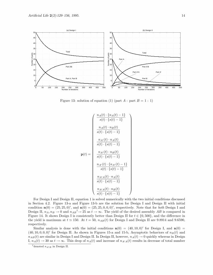
For Design I and Design II, equation 1 is solved numerically with the two initial conditions discussedin Section 4.2. Figure 13-a and Figure 13-b are the solution for Design I and Design II with initialcondition n(0) = (25, 25, 0)′, and n(0) = (25, 25, 0, 0, 0)′, respectively. Note that for both Design I andDesign II, nA, nB → 0 and nAB

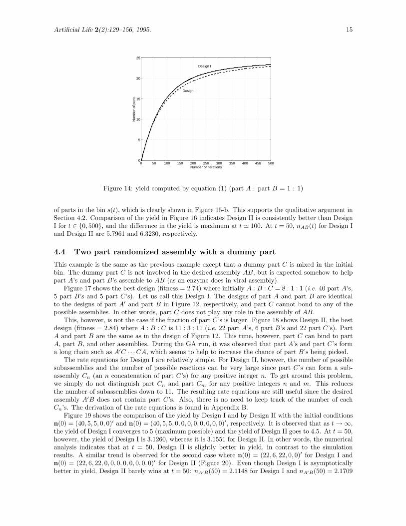
7→ 25 as t → ∞. The yield of the desired assembly AB is compared inFigure 14. It shows Design I is consistently better than Design II for t ∈ {0, 500}, and the difference inthe yield is maximum at t ' 150. At t = 50, nAB(t) for Design I and Design II are 9.8914 and 9.6590,respectively.

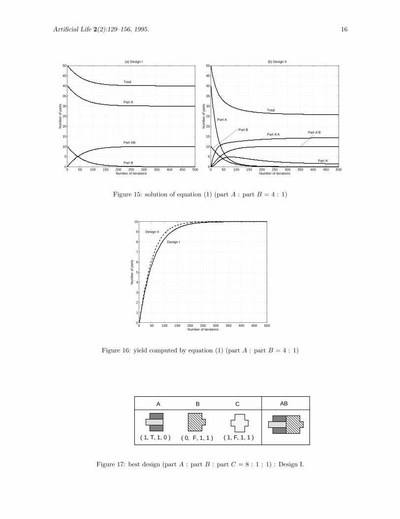
Similar analysis is done with the initial conditions n(0) = (40, 10, 0)′ for Design I, and n(0) =(40, 10, 0, 0, 0)′ for Design II. As shown in Figures 15-a and 15-b, Asymptotic behaviors of nB(t) andnAB(t) are similar in Design I and Design II. In Design II, however, nA(t) → 0 quickly whereas in DesignI, nA(t) → 30 as t → ∞. This drop of nA(t) and increase of nA′A(t) results in decrease of total number

7denoted nA′B in Design II.

Artificial Life 2(2):129–156, 1995. 15

0 50 100 150 200 250 300 350 400 450 5000

5

10

15

20

25

Number of iterations

Num

ber

of p

arts

Design I

Design II

Figure 14: yield computed by equation (1) (part A : part B = 1 : 1)

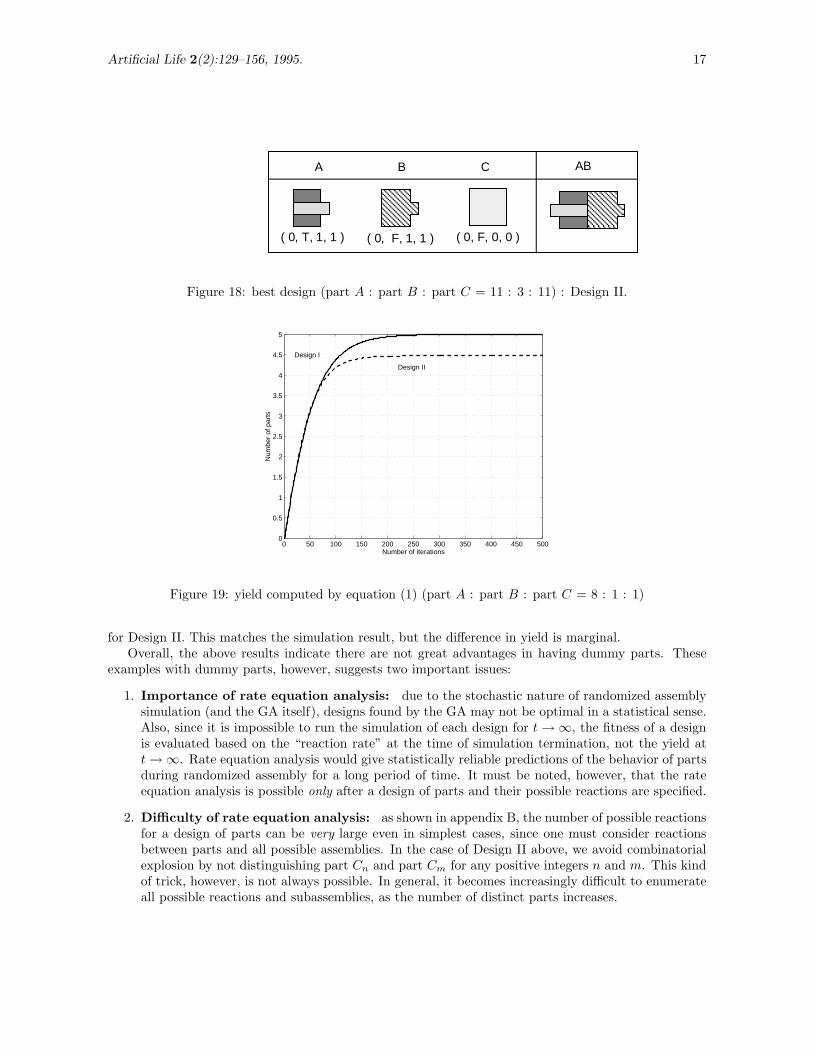
of parts in the bin s(t), which is clearly shown in Figure 15-b. This supports the qualitative argument inSection 4.2. Comparison of the yield in Figure 16 indicates Design II is consistently better than DesignI for t ∈ {0, 500}, and the difference in the yield is maximum at t ' 100. At t = 50, nAB(t) for Design Iand Design II are 5.7961 and 6.3230, respectively.

4.4 Two part randomized assembly with a dummy part

This example is the same as the previous example except that a dummy part C is mixed in the initialbin. The dummy part C is not involved in the desired assembly AB, but is expected somehow to helppart A’s and part B’s assemble to AB (as an enzyme does in viral assembly).

Figure 17 shows the best design (fitness = 2.74) where initially A : B : C = 8 : 1 : 1 (i.e. 40 part A’s,5 part B’s and 5 part C’s). Let us call this Design I. The designs of part A and part B are identicalto the designs of part A′ and part B in Figure 12, respectively, and part C cannot bond to any of thepossible assemblies. In other words, part C does not play any role in the assembly of AB.

This, however, is not the case if the fraction of part C’s is larger. Figure 18 shows Design II, the bestdesign (fitness = 2.84) where A : B : C is 11 : 3 : 11 (i.e. 22 part A’s, 6 part B’s and 22 part C’s). PartA and part B are the same as in the design of Figure 12. This time, however, part C can bind to partA, part B, and other assemblies. During the GA run, it was observed that part A’s and part C’s forma long chain such as A′C · · ·CA, which seems to help to increase the chance of part B’s being picked.

The rate equations for Design I are relatively simple. For Design II, however, the number of possiblesubassemblies and the number of possible reactions can be very large since part C’s can form a sub-assembly Cn (an n concatenation of part C’s) for any positive integer n. To get around this problem,we simply do not distinguish part Cn and part Cm for any positive integers n and m. This reducesthe number of subassemblies down to 11. The resulting rate equations are still useful since the desiredassembly A′B does not contain part C’s. Also, there is no need to keep track of the number of eachCn’s. The derivation of the rate equations is found in Appendix B.

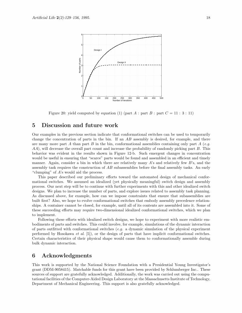
Figure 19 shows the comparison of the yield by Design I and by Design II with the initial conditionsn(0) = (40, 5, 5, 0, 0)′ and n(0) = (40, 5, 5, 0, 0, 0, 0, 0, 0, 0, 0)′, respectively. It is observed that as t → ∞,the yield of Design I converges to 5 (maximum possible) and the yield of Design II goes to 4.5. At t = 50,however, the yield of Design I is 3.1260, whereas it is 3.1551 for Design II. In other words, the numericalanalysis indicates that at t = 50, Design II is slightly better in yield, in contrast to the simulationresults. A similar trend is observed for the second case where n(0) = (22, 6, 22, 0, 0)′ for Design I andn(0) = (22, 6, 22, 0, 0, 0, 0, 0, 0, 0, 0)′ for Design II (Figure 20). Even though Design I is asymptoticallybetter in yield, Design II barely wins at t = 50: nA′B(50) = 2.1148 for Design I and nA′B(50) = 2.1709

Artificial Life 2(2):129–156, 1995. 16

0 50 100 150 200 250 300 350 400 450 5000

5

10

15

20

25

30

35

40

45

50(a) Design I

Number of iterations

Num

ber

of p

arts

Total

Part A

Part B

Part AB

0 50 100 150 200 250 300 350 400 450 5000

5

10

15

20

25

30

35

40

45

50(b) Design II

Number of iterations

Num

ber

of p

arts

Part A

Part B

Part A’

Part A’APart A’B

Total

Figure 15: solution of equation (1) (part A : part B = 4 : 1)

0 50 100 150 200 250 300 350 400 450 5000

1

2

3

4

5

6

7

8

9

10

Number of iterations

Num

ber

of p

arts

Design II

Design I

Figure 16: yield computed by equation (1) (part A : part B = 4 : 1)

BA ABC

( 1, T, 1, 0 ) ( 0, F, 1, 1 ) ( 1, F, 1, 1 )

Figure 17: best design (part A : part B : part C = 8 : 1 : 1) : Design I.

Artificial Life 2(2):129–156, 1995. 17

BA ABC

( 0, T, 1, 1 ) ( 0, F, 1, 1 ) ( 0, F, 0, 0 )

Figure 18: best design (part A : part B : part C = 11 : 3 : 11) : Design II.

0 50 100 150 200 250 300 350 400 450 5000

0.5

1

1.5

2

2.5

3

3.5

4

4.5

5

Number of iterations

Num

ber

of p

arts

Design I

Design II

Figure 19: yield computed by equation (1) (part A : part B : part C = 8 : 1 : 1)

for Design II. This matches the simulation result, but the difference in yield is marginal.Overall, the above results indicate there are not great advantages in having dummy parts. These

examples with dummy parts, however, suggests two important issues:

1. Importance of rate equation analysis: due to the stochastic nature of randomized assemblysimulation (and the GA itself), designs found by the GA may not be optimal in a statistical sense.Also, since it is impossible to run the simulation of each design for t → ∞, the fitness of a designis evaluated based on the “reaction rate” at the time of simulation termination, not the yield att → ∞. Rate equation analysis would give statistically reliable predictions of the behavior of partsduring randomized assembly for a long period of time. It must be noted, however, that the rateequation analysis is possible only after a design of parts and their possible reactions are specified.

2. Difficulty of rate equation analysis: as shown in appendix B, the number of possible reactionsfor a design of parts can be very large even in simplest cases, since one must consider reactionsbetween parts and all possible assemblies. In the case of Design II above, we avoid combinatorialexplosion by not distinguishing part Cn and part Cm for any positive integers n and m. This kindof trick, however, is not always possible. In general, it becomes increasingly difficult to enumerateall possible reactions and subassemblies, as the number of distinct parts increases.

Artificial Life 2(2):129–156, 1995. 18

0 50 100 150 200 250 300 350 400 450 5000

1

2

3

4

5

6

Number of iterations

Num

ber

of p

arts

Design I

Design II

Figure 20: yield computed by equation (1) (part A : part B : part C = 11 : 3 : 11)

5 Discussion and future work

Our examples in the previous section indicate that conformational switches can be used to temporarilychange the concentration of parts in the bin. If an AB assembly is desired, for example, and thereare many more part A than part B in the bin, conformational assemblies containing only part A (e.g.AA), will decrease the overall part count and increase the probability of randomly picking part B. Thisbehavior was evident in the results shown in Figure 12-b. Such emergent changes in concentrationwould be useful in ensuring that “scarce” parts would be found and assembled in an efficient and timelymanner. Again, consider a bin in which there are relatively many A’s and relatively few B’s, and theassembly task requires the construction of AB subassemblies before the final assembly tasks. An early“clumping” of A’s would aid the process.

This paper described our preliminary efforts toward the automated design of mechanical confor-mational switches. We assumed an idealized (yet physically meaningful) switch design and assemblyprocess. Our next step will be to continue with further experiments with this and other idealized switchdesigns. We plan to increase the number of parts, and explore issues related to assembly task planning.As discussed above, for example, how can we impose constraints that ensure that subassemblies arebuilt first? Also, we hope to evolve conformational switches that embody assembly precedence relation-ships. A container cannot be closed, for example, until all of its contents are assembled into it. Some ofthese succeeding efforts may require two-dimensional idealized conformational switches, which we planto implement.

Following these efforts with idealized switch designs, we hope to experiment with more realistic em-bodiments of parts and switches. This could involve, for example, simulations of the dynamic interactionof parts outfitted with conformational switches (e.g. a dynamic simulation of the physical experimentperformed by Hosokawa et al. [5]), or the design of parts that have implicit conformational switches.Certain characteristics of their physical shape would cause them to conformationally assemble duringbulk dynamic interaction.

6 Acknowledgments

This work is supported by the National Science Foundation with a Presidential Young Investigator’sgrant (DDM-9058415). Matchable funds for this grant have been provided by Schlumberger Inc.. Thesesources of support are gratefully acknowledged. Additionally, the work was carried out using the compu-tational facilities of the Computer-Aided Design Laboratory at the Massachusetts Institute of Technology,Department of Mechanical Engineering. This support is also gratefully acknowledged.

Artificial Life 2(2):129–156, 1995. 19

References

[1] S. Casjens. and J. King. Virus assembly. Annual Review of Biochemistry, 44:555–611, 1975.

[2] M. B. Cohn, C. J. Kim, and A. P. Pisano. Self-assembling electrical networks: an application ofmicromachining technology. In Transducers ’91: 1991 Sixth International Conference on Solid-StateSensors and Actuators, pages 490–493, New York, New York, 1991. IEEE.

[3] N. S. Goel and R. L. Thompson. Computer Simulations of Self-organization in Biological Systems.Croom Helm, London, England, 1988.

[4] D. E. Goldberg. Genetic Algorithms in Search, Optimization and Machine Learning. Addison-Wesley, 1989.

[5] K. Hosokawa, I. Shimoyama, and H. Miura. Dynamics of self-assembling systems: Analogy withchemical kinetics. Artificial Life, 1(4):413–427, 1994.

[6] P. H. Moncevicz. Orientation and insertion of randomly presented parts using vibratory agitation.Master’s thesis, Department of Mechanical Engineering, Massachusetts Institute of Technology,1991.

[7] P. H. Moncevicz and M. J. Jakiela. Method and appratus for automatic parts assembly. UnitedStates Patent 5,155,895, October 20 1992.

[8] P. H. Moncevicz, M. J. Jakiela, and K. T. Ulrich. Orientation and insertion of randomly presentedparts using vibratory agitation. In A. H. Soni, editor, Proceedings of the ASME 3rd Conference onFlexible Assembly Systems, pages 41–47, Miami, Florida, September 1991. The American Societyof Mechanical Engineers. DE-Vol. 33.

[9] L. S. Penrose. Self-reproducing machines. Scientific American, 200:105–114, June 1959.

[10] J. I. Steinfeld, J. S. Francisco, and W. L. Hase. Chemical Kinetics and Dynamics. Prentice Hall,Englewood Cliffs, New Jersey, 1989.

[11] R. L. Thompson and N. S. Goel. A simulation of T4 bacteriophage assembly and operation. BioSys-tems, 18:23–45, 1985.

[12] R. L. Thompson and N. S. Goel. Movable finite automata (MFA) models for biological systems I:Bacteriophage assembly and operation. Journal of Theoretical Biology, 131:351–385, 1988.

[13] J. D. Watson, Nancy H. Hopkins, Jeffrey W. Roberts, Joan A. Steitz, and Alan M. Weiner. MolecularBiology of the Gene. Benjamin/Cummings, Menlo Park, California, 1987.

[14] H. J. Yeh and J. S. Smith. Fluidic self-assembly of GaAs microstructures on Si substrates. Sensorsand Materials, 6(6):319–332, 1994.

A Optimal designs of two part non-randomized assembly

This appendix lists all the possible designs that score the maximum fitness (fitness = 2) in the twopart non-randomized assembly discussed in Section 4.1. The length of the chromosome in this exampleis 14 (6 for part A and part B, and 2 for part Z), so there are 214 = 16384 possible chromosomes.Since the assembly process is deterministic, depth first search can find all the optimal solutions withlittle enumeration. They are listed in Figures 21 and 22. Due to the degeneracy of parameter coding(see Section 3.2), more than one chromosome maps to a design. Also, some designs are functionallyequivalent. Figure 22 shows such designs equivalent to the two designs of part B appearing in Figure 21.Since (0, F, 0, 0) has 4 equivalent part designs and (1, F, 0, 0) has 3 equivalent designs, there are4 × 5 + 4 × 4 = 36 optimal designs.

Artificial Life 2(2):129–156, 1995. 20

BAZ

( 0, F, 0, 0 )( 0, T, 1, 1)( 0 )

AB

( 0, F, 0, 0 )( -1, T, 1, 1)( 1 )

( 0, F, 0, 0 )( 0, T, 1, 0 )( 1 )

( 0, F, 0, 0 )( 1, T, 1, 0 )( 0 )

( 1, F, 0, 0 )( 0, T, 1, 0)( 0 )

( 1, F, 0, 0 )( 1, T, 1, -1)( 0 )

BAZ AB

( 1, F, 0, 0 )( -1, T, 1, 0)( 1 )

( 1, F, 0, 0 )( 0, T, 1, -1)( 1 )

Figure 21: optimal designs for two-part non-randomized assembly

Artificial Life 2(2):129–156, 1995. 21

( 0, F, 0, 1 )( 0, F, 0, -1) ( 0, T, 0, 0 ) ( 0, T, 1, 1 )

( 0, F, 1, -1) ( 0, F, 1, 1 )

( 0, F, 0, 0 )

( 0, F, 1, 0 )

( 1, F, 0, 1 )( 1, F, 0, -1) ( 1, T, 1, 1 )( 1, F, 0, 0 )

( 1, F, 1, 0 ) ( 1, F, 1, -1) ( 1, F, 1, 1 )

equivalent designs of part B

Figure 22: equivalent designs of part B

B Rate equation analysis of two part randomized assembly witha dummy part

This appendix explains details of rate equation analysis of two part randomized assembly with a dummypart discussed in Section 4.4. In the following, Design I and Design II refer to the part designs describedin Section 4.4, unless otherwise specified. Derivation of the rate equations of these part designs followsthe same steps found in Section 4.3.

The possible reactions for Design I are:

A + A → AA′ A + B → AB AA′ + B → A + AB

where A′ denotes a part A after conformational change. And n(t), A and p(t) are:

n(t) =

nA(t)nB(t)nC(t)

nAA′(t)nAB(t)

, A =

−2 −1 10 −1 −10 0 01 0 −10 1 1

, p(t) =

nA(t) · {nA(t) − 1}s(t) · {s(t) − 1}

nA(t) · nB(t)

s(t) · {s(t) − 1}

nAA′(t) · nB(t)

s(t) · {s(t) − 1}

As easily seen in Figure 18, the number of possible reactions (and the number of possible subassem-blies) can be very large for Design II since part C’s can form a subassembly Cn (an n concatenation ofpart C’s) up to 22 elements long. Fortunately, C is a solid part so there are no conformational changesin C: once a C binds to another C, the bond will never be destroyed. The resulting assembly CC willthen behave exactly as a single C. This leads to the idea of not distinguishing part Cn and part Cm forany positive integer n and m. This reduces the number of subassemblies down to 11. The resulting rateequations are still useful since the desired assembly A′B does not contain part C’s. Therefore there isno need to keep track of the number of each Cn’s. Under the above assumption, there are 36 possible

Artificial Life 2(2):129–156, 1995. 22

reactions of Design II:

A + A → A′A A′ + B → A′B A′Cn + CnA → A′CnAA + B → A′B A′ + Cn → A′Cn A′Cn + CnB → A′CnBA + Cn → A′Cn A′ + A′ → A′A CnA + A → Cn + A′AA + CnA → A′CnA A′A + A → A′ + A′A CnA + B → Cn + A′BA + CnB → A′CnB A′A + B → A′ + A′B CnA + Cn → Cn + A′Cn

Cn + A → CnA A′A + Cn → A′ + A′Cn CnA + CnA → Cn + A′CnACn + B → CnB A′A + CnA → A′ + A′CnA CnA + CnB → Cn + A′CnBCn + Cn → Cn A′A + CnB → A′ + A′CnB A′CnA + A → A′Cn + A′ACn + A′ → CnA A′Cn + A → A′CnA A′CnA + B → A′Cn + A′BCn + CnA → CnA A′Cn + B → A′CnB A′CnA + Cn → A′Cn + A′Cn

Cn + CnB → CnB A′Cn + Cn → A′Cn A′CnA + CnA → A′Cn + A′CnAA′ + A → A′A A′Cn + A′ → A′CnA A′CnA + CnB → A′Cn + A′CnB

where A′ denotes a part A after conformational change, and Cn denotes a concatenation of some numberof part C’s. Corresponding n(t), A and p(t) are, therefore, defined as follows:

n(t) = (nA(t), nB(t), nCn(t), nA′(t), nA′A(t), nA′B(t), nA′Cn

(t), nCnA(t), nCnB(t), nA′CnA(t), nA′CnB(t))′

A =

−2 −1 −1 −1 −1 −1 0 0 0 0 0 −1 0 0 0 −1 0 00 −1 0 0 0 0 −1 0 0 0 0 0 −1 0 0 0 −1 00 0 −1 0 0 −1 −1 −1 −1 −1 −1 0 0 −1 0 0 0 −10 0 0 0 0 0 0 0 −1 0 0 −1 −1 −1 −2 1 1 11 0 0 0 0 0 0 0 0 0 0 1 0 0 1 0 −1 −10 1 0 0 0 0 0 0 0 0 0 0 1 0 0 0 1 00 0 1 0 0 0 0 0 0 0 0 0 0 1 0 0 0 10 0 0 −1 0 1 0 0 1 0 0 0 0 0 0 0 0 00 0 0 0 −1 0 1 0 0 0 0 0 0 0 0 0 0 00 0 0 1 0 0 0 0 0 0 0 0 0 0 0 0 0 00 0 0 0 1 0 0 0 0 0 0 0 0 0 0 0 0 00 0 −1 0 0 0 0 0 −1 0 0 0 0 −1 0 0 0 00 0 0 −1 0 0 0 0 0 −1 0 0 0 0 −1 0 0 00 0 0 0 −1 0 0 0 1 1 0 1 1 0 0 −1 0 01 1 0 0 0 −1 0 0 0 0 0 0 0 0 0 0 0 0

−1 −1 0 0 0 0 0 0 1 0 0 0 0 1 0 0 0 00 0 0 0 0 0 0 0 0 1 0 0 0 0 1 0 0 00 0 −1 −1 0 −1 −1 −1 0 0 1 0 0 1 1 2 1 1

−1 0 0 0 0 0 −1 0 −1 −1 −1 −2 −1 0 0 0 −1 00 −1 0 0 0 0 0 −1 0 0 0 0 −1 0 0 0 0 −11 0 1 0 0 1 1 0 0 0 0 1 0 −1 −1 −1 0 −10 1 0 1 0 0 0 1 0 0 0 0 1 0 0 0 0 1

Artificial Life 2(2):129–156, 1995. 23

p1(t) =nA(t) · {nA(t) − 1}

s(t) · {s(t) − 1} p2(t) =nA(t) · nB(t)

s(t) · {s(t) − 1} p3(t) =nA(t) · nCn(t)

s(t) · {s(t) − 1}

p4(t) =nA(t) · nCnA(t)

s(t) · {s(t) − 1} p5(t) =nA(t) · nCnB(t)

s(t) · {s(t) − 1} p6(t) =nCn(t) · nA(t)

s(t) · {s(t) − 1}

p7(t) =nCn(t) · nB(t)

s(t) · {s(t) − 1} p8(t) =nCn(t) · {nCn(t) − 1}

s(t) · {s(t) − 1} p9(t) =nCn(t) · nA′(t)

s(t) · {s(t) − 1}

p10(t) =nCn(t) · nCnA(t)

s(t) · {s(t) − 1} p11(t) =nCn(t) · nCnB(t)

s(t) · {s(t) − 1} p12(t) =nA′(t) · nA(t)

s(t) · {s(t) − 1}

p13(t) =nA′(t) · nB(t)

s(t) · {s(t) − 1} p14(t) =nA′(t) · nCn(t)

s(t) · {s(t) − 1} p15(t) =nA′(t) · {nA′(t) − 1}

s(t) · {s(t) − 1}

p16(t) =nA′A(t) · nA(t)

s(t) · {s(t) − 1} p17(t) =nA′A(t) · nB(t)

s(t) · {s(t) − 1} p18(t) =nA′A(t) · nCn(t)

s(t) · {s(t) − 1}

p19(t) =nA′A(t) · nCnA(t)

s(t) · {s(t) − 1} p20(t) =nA′A(t) · nCnB(t)

s(t) · {s(t) − 1} p21(t) =nA′Cn(t) · nA(t)

s(t) · {s(t) − 1}

p22(t) =nA′Cn(t) · nB(t)

s(t) · {s(t) − 1} p23(t) =nA′Cn(t) · nCn(t)

s(t) · {s(t) − 1} p24(t) =nA′Cn(t) · nA′(t)

s(t) · {s(t) − 1}

p25(t) =nA′Cn(t) · nCnA(t)

s(t) · {s(t) − 1} p26(t) =nA′Cn(t) · nCnB(t)

s(t) · {s(t) − 1} p27(t) =nCnA(t) · nA(t)

s(t) · {s(t) − 1}

p28(t) =nCnA(t) · nB(t)

s(t) · {s(t) − 1} p29(t) =nCnA(t) · nCn(t)

s(t) · {s(t) − 1} p30(t) =nCnA(t) · {nCnA(t) − 1}

s(t) · {s(t) − 1}

p31(t) =nCnA(t) · nCnB(t)

s(t) · {s(t) − 1} p32(t) =nA′CnA(t) · nA(t)

s(t) · {s(t) − 1} p33(t) =nA′CnA(t) · nB(t)

s(t) · {s(t) − 1}

p34(t) =nA′CnA(t) · nCn(t)

s(t) · {s(t) − 1} p35(t) =nA′CnA(t) · nCnA(t)

s(t) · {s(t) − 1} p36(t) =nA′CnA(t) · nCnB(t)

s(t) · {s(t) − 1}

For Design I and Design II, equation 1 is solved numerically with the two initial conditions discussedin Section 4.4. Figure 23 and Figure 24 are the solutions for Design I and Design II with initial conditionn(0) = (40, 5, 5, 0, 0)′, and n(0) = (40, 5, 5, 0, 0, 0, 0, 0, 0, 0, 0)′, respectively. The same analysis is donewith initial condition n(0) = (22, 6, 22, 0, 0)′ for Design I, and n(0) = (22, 6, 22, 0, 0, 0, 0, 0, 0, 0, 0)′ forDesign II. These results are shown in Figure 25 and Figure 26.

Artificial Life 2(2):129–156, 1995. 24

0 50 100 150 200 250 300 350 400 450 5000

5

10

15

20

25

30

35

40

45

50Design I

Number of iterations

Num

ber

of p

arts

Part A

Part B

Part CPart AA’

Part AB

Total

Figure 23: solution of equation (1) for Design I (part A : part B : part C = 8 : 1 : 1)

0 50 100 150 200 250 300 350 400 450 5000

5

10

15

20

25

30

35

40

45

50(a) Design II: N_A, N_B, N_Cn, N_A’, N_A’A, N_A’B, N_total

Number of iterations

Num

ber

of p

arts

Part A

Part B

Part Cn

Part A’

Part A’A

Part A’B

Total

0 50 100 150 200 250 300 350 400 450 5000

0.5

1

1.5

2

2.5

3

3.5(b) Design II: N_A’Cn, N_CnA, N_CnB, N_A’CnA, N_A’CnB

Number of iterations

Num

ber

of p

arts

Part A’Cn

Part CnA

Part CnB

Part A’CnB

Part A’CnA

Figure 24: solution of equation (1) for Design II (part A : part B : part C = 8 : 1 : 1)

Artificial Life 2(2):129–156, 1995. 25

0 50 100 150 200 250 300 350 400 450 5000

5

10

15

20

25

30

35

40

45

50Design I

Number of iterations

Num

ber

of p

arts

Part A

Part B

Part C

Part AA’Part AB

Total

Figure 25: solution of equation (1) for Design I (part A : part B : part C = 11 : 3 : 11)

0 50 100 150 200 250 300 350 400 450 5000

5

10

15

20

25

30

35

40

45

50(a) Design II: N_A, N_B, N_Cn, N_A’, N_A’A, N_A’B, N_total

Number of iterations

Num

ber

of p

arts

Part A

Part B

Part Cn

Part A’Part A’A

Part A’B

Total

0 50 100 150 200 250 300 350 400 450 5000

1

2

3

4

5

6(b) Design II: N_A’Cn, N_CnA, N_CnB, N_A’CnA, N_A’CnB

Number of iterations

Num

ber

of p

arts

Part A’Cn

Part CnA

Part CnB

Part A’CnA

Part A’CnB

Figure 26: solution of equation (1) for Design II (part A : part B : part C = 11 : 3 : 11)