Automated Geophysical Feature Detection with Deep Learning

Chiyuan Zhang, Charlie Frogner and Tomaso Poggio, MIT.Mauricio Araya-Polo, Jan Limbeck and Detlef Hohl, Shell International

Exploration & Production Inc.GPU Technology Conference 2016, April 4~7

MotivationMotivation ↔ Methods ↔ Results

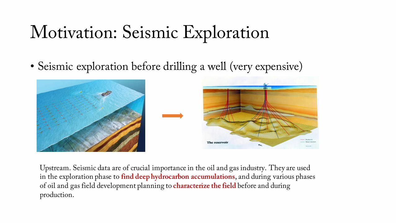
Motivation: Seismic Exploration• Seismic exploration before drilling a well (very expensive)

Upstream. Seismic data are of crucial importance in the oil and gas industry. They are used in the exploration phase to find deep hydrocarbon accumulations, and during various phases of oil and gas field development planning to characterize the field before and during production.

Seismic Survey WorkflowData acquisition, on/off shore.

Data processing: iterations could take multiple months with human experts.

Seismic traceswaveforms (time series) indexed

by shot id and receiver id

Automated Geophysical Feature Detection

Step 1: Interpretation & Modeling

Step 2: Feedback loop & Iterations

Geophysical Features & Structures

Automated Geophysical Feature Detection

Step 1: Interpretation & Modeling

Step 2: Feedback loop & Iterations

Geophysical Features & Structures

Early stages feature detection can help to steer the interpretation & modeling process.

Automated Geophysical Feature Detection

Seismic Survey

Machine Learning

From raw seismic traces, discover (classification) and locate (structured prediction) faults in the underground structure, before running migration / interpretation.

MethodsMotivation ↔ Methods ↔ Results

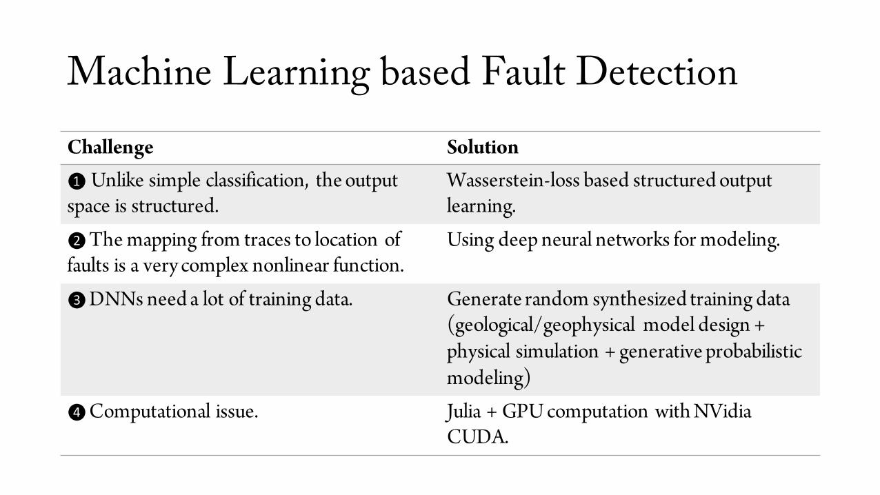
Machine Learning based Fault DetectionChallenge Solution❶ Unlike simple classification, the output space is structured.

Wasserstein-loss based structured output learning.

❷The mapping from traces to location of faults is a very complex nonlinear function.

Using deep neural networks for modeling.

❸DNNs need a lot of training data. Generate random synthesized training data (geological/geophysical model design + physical simulation + generative probabilistic modeling)

❹Computational issue. Julia + GPU computation with NVidia CUDA.

Learning with Wasserstein Loss• The machine learning task• Classification & structured-output prediction• Wasserstein-loss [FZMAP15] to enforce

smoothness in the output space

• Difference between object-detection like tasks in computer vision:• Input (time-series at different sensor location) and

output (spatial map) live in different domain.• Time-location correspondence is unknown until full

migration / interpretation is done.

FZMAP15: C. Frogner*, C. Zhang*, H. Mobahi, M. Araya-Polo, T. Poggio. Learning with a Wasserstein Loss. NIPS 2015.

Deep Learning based Fault Detection

DataWarehouse

Deep Neural Networks

AsynchronizedData IO

GPU Parallel ComputingCPUStochastic Gradient

Descent Solver Scheduling

MIT JuliaNVidia cuDNN

Synthesizing Training DataSynthesize Random

Velocity Models

Simulate Wave-propagation & Collect Seismic Traces

Generate Ground-truth Fault Location

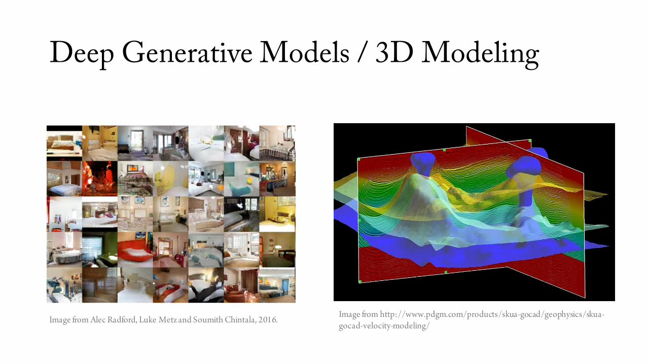
Deep Generative Models / 3D Modeling

Image from Alec Radford, Luke Metz and Soumith Chintala, 2016. Image from http://www.pdgm.com/products/skua-gocad/geophysics/skua-gocad-velocity-modeling/

Deep Learning on GPUshidden_layers = map(1:n_hidden_layer) do i

InnerProductLayer(name="ip$i", output_dim=n_units_hidden, bottoms=[i == 1 ? :data : symbol("ip$(i-1)")],tops=[symbol("ip$i")],weight_cons=L2Cons(10),neuron = neuron == :relu ? Neurons.ReLU() : Neurons.Sigmoid())

endpred_layer = InnerProductLayer(name="pred", output_dim=n_class,

tops=[:pred], bottoms=[symbol("ip$n_hidden_layer")])loss_layer = WassersteinLossLayer(bottoms=[:predsoft, :label])

backend = use_gpu ? GPUBackend() : CPUBackend()method = SGD()params = make_solver_parameters(method)solver = Solver(method, params)

libcudaRTlibcuBLASlibcuRANDlibcuDNN

Summary of Challenges & Solutions

DataWarehouse

Mocha.jlJulia-based deep learning

toolkit

Wasserstein LossLoss function with semantic

smoothness

Deep Neural Networks

Multi-layer dense layers

ComputationBackends

CPU, GPU (cuDNN)

❶

❷❸

❹

ResultsMotivation ↔ Methods ↔ Results

Results: Plots, single faultTest case: 10k models, 510k traces, SGD 250k iterations. No noise, 1 fault, no salt body, downsample 64. DNN arch: 4 layers,1024 neurons

Prediction accuracy:• Area under Curve (AUC): 77%• Intersection over Union (IOU): 71%

Results: Plots, multiple faultsTest case: 10k models, 510k traces, SGD 250k iterations. No noise, 2 faults, no salt body, downsample 8. DNN arch: 4 layer, 768 neurons

Prediction accuracy:• Area under Curve (AUC): 86%• Intersection over Union (IOU): 75%

Results: Plots, salt bodiesTest case: 10k models, 510k traces, SGD 250k iterations. No noise, 1 fault, Salt body, downsample 8. DNN arch: 2, 256

Prediction accuracy:• Area under Curve (AUC): 96%• Intersection over Union (IOU): 74%

Results: Computation Performance• Performance plots, test case 10k models (80/20 split)

• CPU vs GPU: for the same reference architecture our GPU (1 chip of a K80) implementation is 38x faster than the CPU one (1 Haswell E5-2680, 12 cores)

• Multi-GPU. We are collaborating with BitFusion (booth 731) to get this feature at Mocha level, so then transparent for our architectures

4 layers768 neurons

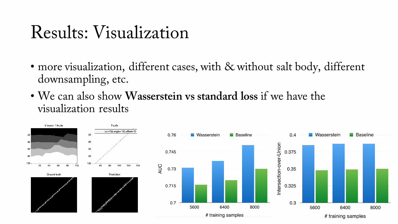
Results: Visualization• more visualization, different cases, with & without salt body, different

downsampling, etc.• We can also show Wasserstein vs standard loss if we have the

visualization results

Summary• Deep-learning based system for automate geophysical feature

detection from pre-migrated raw data.• Generative model + physical simulation of wave propagation for

synthesized training data.• Wasserstein-loss for structured output learning problems.• GPU-accelerated computation for fast modeling.