Automated Generation of Kempe Linkages for Algebraic ...akobel/publications/Kobel08-kempe... ·...
56
Bachelor‘s Thesis in Computer Science Automated Generation of Kempe Linkages for Algebraic Curves in a Dynamic Geometry System submitted by Alexander Kobel on September 26, 2008 U N IV E R S I T A S S A R A V I E N S I S Saarland University, Saarbr¨ ucken, Germany Faculty of Natural Sciences and Technology I Department of Computer Science Supervisor and First Reviewer Prof. Dr. Frank-Olaf Schreyer Advisor and Second Reviewer Dr. Oliver Labs
Transcript of Automated Generation of Kempe Linkages for Algebraic ...akobel/publications/Kobel08-kempe... ·...
Bachelor‘s Thesis in Computer Science
Automated Generation
of Kempe Linkages for Algebraic Curves
in a Dynamic Geometry System
submitted by
Alexander Kobel
on September 26, 2008
UN
IVE R S IT A
S
SA
RA V I E N
SI S
Saarland University, Saarbrucken, GermanyFaculty of Natural Sciences and Technology I
Department of Computer Science
Supervisor and First Reviewer
Prof. Dr. Frank-Olaf Schreyer
Advisor and Second Reviewer
Dr. Oliver Labs

Non-plagiarism statement
Hereby I confirm that this thesis is my own work and that I have documented allsources used.
Statement of Consistence
Hereby I confirm that this thesis is identical to the digital version submitted at the sametime.
Declaration of Consent
Herewith I agree that my thesis will be made available through the library of theComputer Science Department.
Saarbrucken, September 26, 2008
Alexander Kobel


Abstract
In 1876, Alfred Bray Kempe stated a preliminary version of what nowadays is knownas Kempe‘s Universality Theorem: For any intersection of an algebraic curve with aclosed disc in the Euclidean real plane R2, there is a linkage translating a motion alongthese curve segments to a straight line segment and vice-versa. Using linkages like thePeaucellier inversor, which constrain a hinge to a straight line segment, it is thus possibleto piecewise delineate arbitrary algebraic curves. This is particularly remarkable incombination with the Stone-Weierstraß approximation theorem, which states thatarbitrary continuous functions or curves inside a compact set can be interpolated inany precision by polynomial functions or algebraic curves.
In this thesis, we present the constructions involved in assembling those linkages,following Kempe‘s original approach and a more recent reformulation by Gao et al. Inaddition, we shortly outline some recent results by Abbott et al. on generalizations ofKempe‘s Universality Theorem to arbitrary dimensions.
The writing comes along with an implementation of a one-way simulation of thelinkage design in a dynamical geometry system called Cinderella, which featuresso far unrivaled mathematical background for ruler-compass constructions withoutspecialization to particular applications. “One-way” here refers to the translation froma movement on the curve to the straight line.
Information on the shape of the algebraic curve is retrieved via an Internet interfacefrom the ongoing project Xalci, provided by the Algorithms and Complexity workinggroup of the Max-Planck Institute for Computer Science. Their work aims on thetopological analysis and visualization of implicit algebraic curves while providingguaranteed exactness of the results, and is to be extended for algebraic surfaces andcurves in higher dimensions.
Our simulation tries to give as much freedom to the user as possible, within thelimits set by computational complexity of a theoretically perfectly general approach. Asof the publishing of this thesis in the end of September 2008, the interface is publiclyavailable at http://www.math.uni-sb.de/ag/schreyer/Kempe-Linkage/.
i

Acknowledgements
Behind the scenes of this thesis there are a lot of patient and helpful people, who havespent time and work in my favor. I want to mention the most important ones here andthank them for their support, not only while I was writing this thesis, but during mywhole studies.
The first to mention is Timo von Oertzen, who led me on my first steps of the way intoalgebraic geometry—probably without even knowing about this.
At this time, he was employed as an assistant of Frank-Olaf Schreyer, who assured meto again care about maths, motivated me by giving interesting lectures, and eventuallyagreed to supervise me for the writing of this thesis.
The topic of the latter was proposed by Timo‘s successor Oliver Labs. Not only myadvisor and the person to speak to when you have issues with anything in geometry,he also knows the right persons to call for help: Ulrich Kortenkamp, the main author ofCinderella, and Pavel Emeliyanenko and the Algorithms and Complexity working group at theMax-Planck-Institute for Computer Science, without whom the accompanying practicalpart of this thesis would not have been possible to do.
Besides, Oliver also is someone you want to have a chat with for a cup of coffee.This eventually leads to the Teestube of the departement of mathematics in Saarbrucken,where—despite it‘s name—you have a hard time looking for tea, but you always getcoffee. Lately this is Daniel Fries merit, being the donator of a Senseo coffee maker.Along with Andreas Fromkorth and Tobias Schnur, he is one of the many “inhabitants”of the Teestube to mention here for being the partners of hours of fruitful discussions,although not always on mathematics, who so helped me to find my way to and throughthis thesis.
ii

iii


Contents
1 Introduction 1
1.1 Kempe Linkages . . . . . . . . . . . . . . . . . . . . . . . . . . . . . . . . 1
1.2 Dynamic Geometry in Cinderella . . . . . . . . . . . . . . . . . . . . . . . 2
1.3 Algebraic Geometry Visualization in Xalci . . . . . . . . . . . . . . . . . 3
2 Basic Linkages 5
2.1 Straight Line Motion . . . . . . . . . . . . . . . . . . . . . . . . . . . . . . 5
2.1.1 How to Draw a Straight Line? . . . . . . . . . . . . . . . . . . . . 5
2.1.2 An Inexact Approach: Watt‘s linkage . . . . . . . . . . . . . . . . 6
2.1.3 An Exact Solution: The Peaucellier-Lipkin Cell . . . . . . . . . . 7
2.1.4 The Peaucellier Cell on Slot . . . . . . . . . . . . . . . . . . . . . . 9
2.2 The Translator . . . . . . . . . . . . . . . . . . . . . . . . . . . . . . . . . . 9
2.3 The Rotator . . . . . . . . . . . . . . . . . . . . . . . . . . . . . . . . . . . 10
2.3.1 The Distance Copier . . . . . . . . . . . . . . . . . . . . . . . . . . 11
2.4 Angle Adder and Multiplicator . . . . . . . . . . . . . . . . . . . . . . . . 12
2.4.1 The Angle Adder . . . . . . . . . . . . . . . . . . . . . . . . . . . . 12
2.4.2 The Angle Multiplicator . . . . . . . . . . . . . . . . . . . . . . . . 12
3 Kempe Linkages for Plane Curves 15
3.1 Trigonometric Algebra . . . . . . . . . . . . . . . . . . . . . . . . . . . . . 15
3.2 Kempe‘s Straight Line Linkwork . . . . . . . . . . . . . . . . . . . . . . . 18
3.3 Complexity of the Kempe Linkage . . . . . . . . . . . . . . . . . . . . . . 20
3.4 Generalizations and Criticism of Kempe‘s Proof and Open Questions . 22
4 Simulation of Kempe Linkages using Cinderella and Xalci 25
4.1 Some Design Aspects of Cinderella . . . . . . . . . . . . . . . . . . . . . . 25
4.1.1 Complex Projective Geometry . . . . . . . . . . . . . . . . . . . . 26
4.1.2 Continuity . . . . . . . . . . . . . . . . . . . . . . . . . . . . . . . . 27
4.1.3 Automated Theorem Checking . . . . . . . . . . . . . . . . . . . . 28
4.1.4 CindyScript . . . . . . . . . . . . . . . . . . . . . . . . . . . . . . . 30
v

4.2 Visualization of Implicit Algebraic Curves using Xalci . . . . . . . . . . . 31
4.3 Geometric Primitives in Linkage Simulation . . . . . . . . . . . . . . . . 32
4.4 Presentation of Our Simulation of Kempe Linkages . . . . . . . . . . . . 36
4.4.1 The User Interface . . . . . . . . . . . . . . . . . . . . . . . . . . . 36
4.4.2 Animations . . . . . . . . . . . . . . . . . . . . . . . . . . . . . . . 37
4.4.3 Complicated Curves and Statistics . . . . . . . . . . . . . . . . . . 40
4.5 Conclusion . . . . . . . . . . . . . . . . . . . . . . . . . . . . . . . . . . . . 42
vi

List of Figures
2.1 Watt‘s linkage . . . . . . . . . . . . . . . . . . . . . . . . . . . . . . . . . . 7
2.2 The Peaucellier-Lipkin cell . . . . . . . . . . . . . . . . . . . . . . . . . . . 8
2.3 The Peaucellier cell on slot . . . . . . . . . . . . . . . . . . . . . . . . . . . 9
2.4 Two translators. . . . . . . . . . . . . . . . . . . . . . . . . . . . . . . . . . 10
2.5 The distance copier . . . . . . . . . . . . . . . . . . . . . . . . . . . . . . . 11
2.6 The angle multiplicator . . . . . . . . . . . . . . . . . . . . . . . . . . . . 13
3.1 The parallelogram defined by P . . . . . . . . . . . . . . . . . . . . . . . . 16
3.2 The final translations of Kempe‘s construction . . . . . . . . . . . . . . . 19
3.3 Three possible configurations of a simple translator linkage . . . . . . . 23
3.4 A braced parallelogram . . . . . . . . . . . . . . . . . . . . . . . . . . . . 23
4.1 The perpendicular bisector of a segment . . . . . . . . . . . . . . . . . . 26
4.2 The intersection of two parallel lines at infinity . . . . . . . . . . . . . . . 27
4.3 The angular bisector in continuous and deterministic geometry systems 27
4.4 Automatic theorem checking in Cinderella . . . . . . . . . . . . . . . . . . 29
4.5 Multiplication and addition of angles . . . . . . . . . . . . . . . . . . . . 34
4.6 Multiplication of lengths . . . . . . . . . . . . . . . . . . . . . . . . . . . . 35
4.7 Division of lengths by application of the intercept theorem . . . . . . . . 35
4.8 The graphical user interface of our implementation . . . . . . . . . . . . 37
4.9 Static screenshots . . . . . . . . . . . . . . . . . . . . . . . . . . . . . . . . 38
4.10 Animation stills of a Kempe linkage simulation of y2 = x2 − x3 . . . . . 39
4.11 Animation stills of a Kempe linkage simulation of y2 = x2 − x3 (cont‘d) 40
4.12 Some complicated examples . . . . . . . . . . . . . . . . . . . . . . . . . . 41
vii

1 Introduction
1.1 Kempe Linkages
A fundamental task of engineering is the problem of assembling mechanisms whichmake a distinct element move along a certain path. While recent achievements inelectrical engineering allow positioning of devices with incredible precision by meansof microcontrollers, larger scale applications still rely on classical solutions: gearsusing shafts, chains, belts or ball bearings can be found in almost every imaginablemechanical part, from wind engines down to the fans in your laptop. Although theconstruction of these parts clearly involves difficulties, like natural restrictions on thesize, the robustness and degree of efficiency is often the telling argument for the use ofthose classical components.
Probably the best known example is James Watt‘s “parallel motion” linkage, datingback to 1784 and employed in early locomotives operated by steam engines. It is usedto convert the linear motion of the piston to drive the rotation of the wheels. Whilethe parallel motion almost perfectly answers it‘s purpose, it is far from a theoreticallyperfect solution on the translation of a straight line to a circle.
In 1876, Alfred Bray Kempe used the components of Watt‘s engine to develop linkagesto piecewise delineate arbitrary algebraic curves, starting from their implicit polynomialform. Here, a linkage is—like Watt‘s parallel motion—a device assembled of rigidbars of fixed length, connected by hinges on their endpoints. The linkwork translatesto a crank describing a circle, or a straight line, which is proven to be equivalent byCharles-Nicolas Peaucellier‘s invention of the Peaucellier cell which, in contrast to Watt‘slinkage, is capable of exactly converting rotations to linear motions.
Probably the most elegant reformulation of Kempe‘s Universality Theorem, how itis referred to these days, originates from William Thurston. By applying the Stone-Weierstraß approximation theorem, he follows that there is a series of linkworksapproximating any continuous bounded plane curve. Thurston therefore summarizedthat “there is a linkage that signs your name”, assuming you have a finite name.
Kempe slightly criticized Euclid for his stressing of ruler-compass construction
1

1 Introduction
without actually giving a hint how to build an ideal ruler in the first place. Thus,it appears ironical that Kempe himself is best known among mathematicians for hisfalse proof of the four colour theorem, and he also turned out to be careless in hislinkage design. However, both these works rendered a great service to the mathematicalcommunity and have been corrected later; both proofs involve Kempe‘s original keyideas.
With his work, Kempe eventually settled an important question in engineering fromthe theoretical point of view; although he gave a constructive description of the designof the linkwork, the complexity of the mechanisms exceeds the practically relevant limit.It remained an open field to the engineers to figure out easier approximate solutions;however, simulations of the linkages turned out to be useful in modern applications,such as CAD and robotics.
Kempe‘s conclusions have been extended later to arbitrary dimensions. With someadditional restrictions not considered by him, there still is uncharted territory left tofurther research.
1.2 Dynamic Geometry in Cinderella
Everyone of us may with mixed feelings remember the geometry lessons in school.Probably nobody dealt with the class without some torn sheets of paper, with drawingsat the wrong scale or a cluttered choice of parameters for constructions.
Dynamic geometry systems (DGS) tackle this problem, allowing to arbitrarily zoomand shift the viewport or modify some input elements and automatically rearrangethe depending parts accordingly. The current calculating capacity of usual personalcomputers, available at cheap prices and in increasing quantities found in schools,also allow interactive animations and tracing of elements under movements of others,capable of drastically easing the teaching of the relation of mathematics and the “realworld”. Beyond the applications in high school lessons, dynamic geometry programsincreasingly aim to include more in-depth topics, like introductory projective geometry,which demand a great deal of imagination from the student.
Amongst a number of tools mainly targeted at the profitable market of high schoolpupils, Cinderella takes a special position. Throughout the twelve-years developementprocess of Cinderella up to now, the authors Ulrich Kortenkamp and Jurgen Richter-Gebert took great care of implementing a thorough mathematical model of geometry.
Besides features such as polar views on constructions or the representation of hy-perbolic geometry, there are two major differences in design compared to standard
2

1.3 Algebraic Geometry Visualization in Xalci
systems: First, all elements of a Cinderella construction are considered in the complexprojective plane, which guarantees consistency of constructions even in degeneratepositions. Second, Cinderella strictly adheres the concept of continuous movements.Both features are—in this extent—only competed by a discontinued project named“pdb“ (“projective drawing board”) by Harald Winroth, whose workings on dynamicgeometry theory the authors of Cinderella base on. One benefit of this approach is that,up to now, Cinderella is the only dynamic geometry system able to draw complete loci,i.e. traces of objects under continuous movements of others.
An additional advantage of Cinderella for more complex constructions is it‘s embed-ded script editor, which grants the full power of a high-level programming languagewith focus on it‘s geometric operations. Hereby, it spares the user from the neces-sary calculations performed in background—it suffices to deal with the constructionssemantics.
Finally, Cinderella offers the possibility to work embedded in web pages as a Javaapplet, which renders a great opportunity for proof-of-concept presentations.
These outstanding capabilities as well as Kortenkamp‘s offer to support our projectare our reasons to choose Cinderella as the basis for an implementation of Kempe‘salgorithm in a modern geometry environment.
1.3 Algebraic Geometry Visualization in Xalci
Rendering of algebraic curves and surfaces are the main underlying procedures ofalmost every recent geometric modeling application. However this is typically donewithin tight boundaries on the complexity of the mathematical object. Font rendering,standard vector drawing tools or 3D modeling and computer aided design (CAD) usu-ally employ at most nonuniform rational B-spline surfaces (NURBS), which nowadayscan be animated in real-time without major trouble for reasonable input sizes.
Still there is a need for handling higher degree objects without a given parametriza-tion, respecting exactness guarantees on both shape and topology. For example,industrial tools for computer aided manufacturing in specialized high-precision appli-cations have to provide seemless transitions which exceed the possibilities of splineapproximations.
This is the long-term goal of Xalci, part of the EXACUS project for Exact Algorithmson Curves and Surfaces at the Algorithms and Complexity working group of theMax-Planck-Institute for Computer Science in Saarbrucken. Xalci treats the topologicalcorrect analysis of arrangements of implicit algebraic curves, to be extended to also
3
1 Introduction
cover space curves and surfaces. Subsequently, simpler subdivisions with easy topologyare each rasterized independently, giving an exact visualization of the curve up tooutput resolution of the images.
While the algorithms or stand-alone implementations are not publicly available (yet),the results can be seen via a Flash web interface at http://exacus.mpi-inf.mpg.de/cgi-bin/xalci.cgi. This motivated the idea of utilizing the exisiting web transportto gather the shape information of curves needed for rendering and animation of theKempe mechanisms, kindly supported by the Xalci team, in particular represented byPavel Emeliyanenko.
Together with Cinderella‘s web presentation features, we can provide a comprehensivesimulation of the line-curve-translation through a easily usable web interface.
4

2 Basic Linkages
In this chapter, we present basic linkages, which will be our elementary toolkit for themore complicated constructions to follow. We require the reader to be familiar withusual well-known results from elementary geometry; a basic knowledge of algebraicgeometry is assumed throughout the following chapters.
In particular, in section 2.1 we discuss early attempts on describing a straight line bymeans of a linkage. Our goal is the presentation of the Peaucellier-Lipkin cell, a linkagewhich solves this problem exactly. Afterwards, we will express translation of lengths(2.2) as well as rotation (2.3), and addition and multiplication of angles (2.4) in terms ofmechanics.
The linkworks given in this chapter are taken from [GZCG02], and are chosen withtheoretical aspects in mind. Especially the number of links—i.e. the combinatorialcomplexity of the mechanisms—is stressed. For practical applications, a number ofother factors have to be considered, for example the smoothness of movements or thestability of the construction.
For this reason, the linkages presented here are by no means unique. However, forsome akin constructions of similar simplicity, Kempe writes: [Kem77]
In this form, which is a very compact one, the motion has been appliedin a beautiful manner to the air engines which are employed to ventilatethe Houses of Parliament. The ease of working and absence of friction andnoise is very remarkable.
2.1 Straight Line Motion
2.1.1 How to Draw a Straight Line?
The first problem we encounter in finding linkages for algebraic curves seems to bethe most simple case possible: How can we describe a straight line? In fact, this veryproblem is what inspired Kempe to give a lecture about linkages in 1877. In the lecturenotes ([Kem77]) he states
5

2 Basic Linkages
But the straight line, how are we going to describe that? Euclid defines it as“lying evenly between its extreme points.” This does not help us much. Ourtext-books say that the first and second Postulates postulate a ruler. Butsurely that is begging the question. If we are to draw a straight line with aruler, the ruler must itself have a straight edge; and how are we going tomake the edge straight? We come back to our starting point.
To the best of our knowledge, it is not clear whether Euclid itself recognized thisproblem.
For start, we denote that—given a perfect plane—a circle is straightforward to designby linkages. We pick some center point on the plane and stick a pivot there; on thispivot, we attach any kind of rigid material. This allows a circular motion of the shapearound the bolt. We now choose some arbitrary point on the shape; tracing this pointwhile rotating the shape yields, from the theoretical point of view, a perfect circle.
Now the reader might ask where the difference lies in the imagination of a perfectruler and this construction, involving “a perfect plane” and infinitely small “points”and pivots. For our linkage, we are able to adopt the precision according to our needs.In particular, we do not demand the existence of a sample piece of the result. Instead,we rely on basic elements whose overall influence on the relative error of the resultvanishes proportional to the size of the linkage—i.e., the radius of the circle. In a perfectscenario both the pivot and it‘s bearing are circular; however, this is not due to theshape of the curve we want to trace, but a basic requirement for any link of an arbitrarymechanism to achieve smooth transitions.
If we do not have high-precision components for our drawing, we might just takesome branch as pivot and a tensed rope—which essentially fulfills the same require-ments as a rigid shape—and draw a circle in a larger scale, achieving a “roundness”that may well compete today’s industrial parts.
It remains to note that the basic plane is a real restriction; on the other hand, the sameholds for all ruler-compass constructions, so we might have to accept it for granted.
2.1.2 An Inexact Approach: Watt‘s linkage
Despite it‘s seemingly easy nature and high impact on technicial engineering, thestraight-line problem remained unsolved for long time. The best known approach,which was directly influenced by the needs of upcoming technology—namely loco-motives employing a the steam engine—is James Watt‘s Parralel Motion, dating backto 1784. Despite it‘s name, Watt did not succeed in generating parallel curves; in fact,
6

2.1 Straight Line Motion
Figure 2.1: Watt‘s linkage
he could not even solve the straight-line problem. However, for the sake of historicalbackground of linkages, we will shortly explain Watt‘s linkage and the resulting curve.
The linkage (figure 2.1) consists of three bars, consecutively connected by joints. Theouter bars share the same length and are each fixed by pivots on the underlying plane.
Now, we trace the center point of the inner bar under rotation of any of the outerbars. (Of course, it does not matter which one we move, since each determines theposition of the other throughout the motion.)
The resulting curve, called Watt‘s lemniscate, is an algebraic curve of degree six.From a mean position, i.e. a situation where the pencil exactly coincides with the centerof the pivots, the linkage approximates a straight line. The farther we go from themean, the larger gets the deviance from the line; after a full rotation, we end up with aclosed curve. We can thus state that Watt‘s linkage does not allow any configuration todescribe a straight line, because by Bezout‘s theorem a component of an algebraic curvecannot both contain a straight line and at the same time be closed in the real plane R2.
2.1.3 An Exact Solution: The Peaucellier-Lipkin Cell
The first exact solution to the straight-line problem by a planar linkage was given in1864 by Charles-Nicolas Peaucellier. His invention was not recognized by the scientificcommunity in the first place, until Lippman Linkin rediscovered and published hiswork.
The Peaucellier-Lipkin linkage (or just Peaucellier cell) consists of seven bars in a configu-ration as shown in figure 2.2. Here, |AB| = |BC| = |CD| = |DA| = a, |PB| = |PD| = b,and |OP| = |OA| = c. Furthermore, let E be the intersection point of the diagonals ACand BD of the rhombus ABCD.
7

2 Basic Linkages
Figure 2.2: The Peaucellier-Lipkin cell
It holds
|PA| · |PC| = (|PE| − |AE|) · (|PE|+ |AE|)= |PE|2 − |AE|2
= b2 − |BE|2 − |AE|2
= b2 − a2
= const
Thus, C is the inversion point of A with respect to some circle with center P. Theinverse of any circle through P with respect to this circle is a line; in particular, thisholds for the circle centered in O. Therefore, when A rotates around the pivot O, thetrace of C is a straight line perpendicular to PO.
Due to the limited length of the links, the locus of C under all possible configurationsof the linkwork is not a complete line, but a line segment, called a slot. This amountsto performing the necessary calculations in the real numbers. If we consider analgebraically closed field, the resulting curve actually is a line, i.e. the vanishing locusof a two-variate polynomial of degree 1.
In particular, in the complex numbers C, where the Cinderella‘s computations takeplace, the hinges B and D eventually leave the real plane. However, the pencil C stayson a real line. Details as well as a similar example are given in section 4.1.1.
8

2.2 The Translator
Figure 2.3: The Peaucellier cell on slot
2.1.4 The Peaucellier Cell on Slot
We can exploit this limitation of movement to constrain a point in a slot. Starting fromtwo distinct points X and Y, we attach bars of pairwise equal length to get O and P.
The extremal position of the Peaucellier cell occurs if and only if B and D coincideand, thus, the bars AB and BC and likewise AD and DC are on the same line XP (orYP). Accordingly, we choose a = |XP|−c
2 and b = |XP| − a to get a linkage tracing outthe segment XY.
Note that we do not rely an any point on XY but the pivots itself; therefore, we areable to specify the slot without a template.
From now, when we say that a point is in a slot, it means that we use this verymodified Peaucellier linkage to do so. The slot itself still can be moved freely alongwith the attached linkwork; we say that the slot is on a platform determined by X andY.
2.2 The Translator
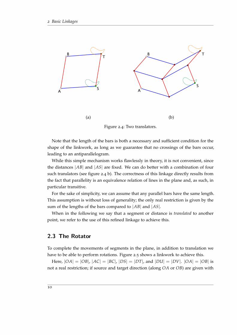
The next tool to be used in linkage design translates a distance to some other place.The most basic idea is to build a parallelogram, in which the bars AB and ST and ASand BT pairwise share the same length. If we attach A and B to some pivots, moving Sin the plane accordingly moves T; ST is a translation of AB.
9
2 Basic Linkages
(a) (b)
Figure 2.4: Two translators.
Note that the length of the bars is both a necessary and sufficient condition for theshape of the linkwork, as long as we guarantee that no crossings of the bars occur,leading to an antiparallelogram.
While this simple mechanism works flawlessly in theory, it is not convenient, sincethe distances |AB| and |AS| are fixed. We can do better with a combination of foursuch translators (see figure 2.4 b). The correctness of this linkage directly results fromthe fact that parallelity is an equivalence relation of lines in the plane and, as such, inparticular transitive.
For the sake of simplicity, we can assume that any parallel bars have the same length.This assumption is without loss of generality; the only real restriction is given by thesum of the lengths of the bars compared to |AB| and |AS|.
When in the following we say that a segment or distance is translated to anotherpoint, we refer to the use of this refined linkage to achieve this.
2.3 The Rotator
To complete the movements of segments in the plane, in addition to translation wehave to be able to perform rotations. Figure 2.5 shows a linkwork to achieve this.
Here, |OA| = |OB|, |AC| = |BC|, |DS| = |DT|, and |DU| = |DV|. |OA| = |OB| isnot a real restriction; if source and target direction (along OA or OB) are given with
10

2.3 The Rotator
Figure 2.5: The distance copier
distinct lengths, say |OB′| > |OA|, we use a platform to constrain B in the slot OB′.Attaching the rotator to the pencil of the Peaucellier linkage accordingly forces a uniqueposition of B where |OA| = |OB|.
In the same manner, S, U, T and V are constrained in OA or OB by platforms. Again,the positions of U, V and, thus, also T are uniquely determined by the position of S init‘s slot.
Now we observe that the construction formed by those restrictions consists of threekites OSDT, OUDV and OACB, which share their axis of symmetry. In particular, OSand OT are the images of each other under mirroring along OC, yielding |OS| = |OT|.
2.3.1 The Distance Copier
Attaching a translator to OT extends this rotator to the distance copier, which assuresthat S′T′ arises as the image of OS under an Euclidean move.
Note that, although the translator is sketched but with a parallelogram, we need themore complex translator (figure 2.4 b) in this situation: in general, we do not know|OS| in advance and thus need the flexibility of distances granted by this translator, notonly to be able to move the linkage, but even to assemble it in a position where all linksfit in the first place.
11

2 Basic Linkages
2.4 Angle Adder and Multiplicator
We finish the presentation of the basic linkworks with two constructions on angleoperations. In particular, we show that linkage designs include all necessary tools toimplement the Z-module structure of angles.
2.4.1 The Angle Adder
A common task in linkage design is the addition of a (finite) number of angles. Thiscan easily be achieved by inductively adding two angles by means of an angle adderconsisting of distance copiers:
Suppose we are given two angles ]AOB and ]CO′D. W.l.o.g. we can assume|OA| = |OB| = |O′C| = |O′D|; otherwise, we use platforms to constrain the linksaccordingly. We then attach two distance copiers to move CO′D such that the imageof O′C is OA, yielding ]CO′D = ]C′O′′D′ = ]AOD′, and now use another distancecopier to move |AB| to D′T such that AB is rotated by the angle ]AOD′ = ]CO′D.
Since we demanded the lengths of the legs to be equal, both AB and AD′ are chordsin a circle with center O. Therefore, ]AOB + ]CO′D = ]AOB + ]AOD′ = ]AOT.
2.4.2 The Angle Multiplicator
Now suppose we want to construct an angle multiplicator, i.e. a mechanism to multiplyan angle by an integer. Again, we can assume both legs to share the same lengths, sowe can use a distance copier in the same manner to double, triple, . . . the angle.
However, there is an easier approach to solve this special case, shown in figure 2.6.Here OADB and OBEC are antiparallelograms; the links satisfy |OA| · |OC| = |OB|2 ⇔|OA||OB| = |OB|
|OC| .
Of course we may not allow |OA| = |OB| in this setting, which leads to the degenerateposition D = 0. This again is not a real restriction, since we can employ platforms toget distinct lengths of the legs. In general, we will have to do so anyway, because wehave to guarantee the ratio of the bar lengths.
Since |OA||OB| = |OB|
|OC| , OADB is similar to OBEC, yielding ]AOB = ]BOC and thus]AOC = ]AOB + ]BOC = 2]AOB. Iterating the construction, we can get a n timesangle multiplicator for arbitrary, but fixed n ∈ N.
Kempe [Kem76] uses the term angle reversor to call the multiplicator, because ]BOA =−]COB; thus the mechanism also allows to change the orientation of arbitrary angles.Together with the angle adder, we are able to subtract angles. As a side remark, which
12

2.4 Angle Adder and Multiplicator
Figure 2.6: The angle multiplicator
is not necessary for our work, we further note that the multiplicator also allows tobisect angles by attaching O, A and C to the relevant points; then, ]AOB = 1
2]AOC.
13


3 Kempe Linkages for Plane Curves
The linkworks presented in chapter 2 are our tools for expressing algebraic terms inmechanisms. We have already seen in the discussion of the Peaucellier inversor that themost basic operation in linkage design is rotation. This suggests that we do better notto describe algebraic curves in the Euclidean plane in Cartesian coordinates as usual,but merely use some variant of a polar coordinate system.
In this chapter we thus explain how to express polynomials and, thus, algebraiccurves by means of trigonometric expressions. We will see that what Abbott et al.[ABD08] call “trigonometric algebra” allows to reduce all occuring terms to somesimple canonical form. In particular, we find out how to cancel arbitrary occurrences ofany variable using linkages attached to only two points, the origin and any chosen unitrepresenting the x-axis.
This directly leads to a constructive proof for Kempe‘s Universality Theorem, whichstates that for every bounded part of a plane algebraic curve there is a linkworkthat translates a motion along the curve to a motion on a straight line segment. Inconsequence, there exists a series of linkworks to delineate any given algebraic curve inany region of the plane.
We close the chapter with a discussion of the complexity of this linkwork, includingsome recent results of Abbott et al. [ABD08], who generalize Kempe‘s work to arbitrarydimensions, and shortly explain their criticism and corrections on Kempe‘s proof.
3.1 Trigonometric Algebra
Throughout this section and the following we give a proof of
Kempe‘s Universality Theorem. Let f ∈ R[x, y] be a polynomial defining an algebraiccurve C = V( f ) =
{(x, y) ∈ R2 : f (x, y) = 0
}, and D be a closed disc in the plane.
Then there exists a linkwork translating a finite motion of a point S along a straight linesegment to a motion of a point P along C ∩ D and vice-versa.
Note that this formulation does not imply a continuous or even connected movement
15
3 Kempe Linkages for Plane Curves
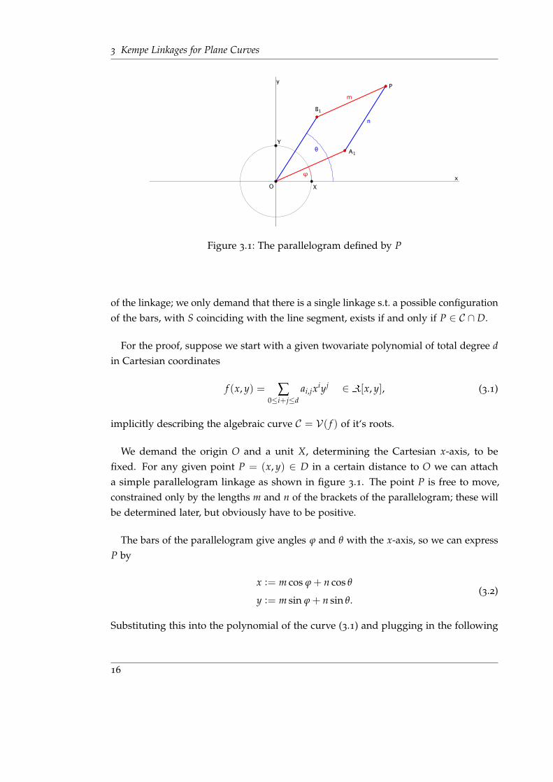
Figure 3.1: The parallelogram defined by P
of the linkage; we only demand that there is a single linkage s.t. a possible configurationof the bars, with S coinciding with the line segment, exists if and only if P ∈ C ∩ D.
For the proof, suppose we start with a given twovariate polynomial of total degree din Cartesian coordinates
f (x, y) = ∑0≤i+j≤d
ai,jxiyj ∈ R[x, y], (3.1)
implicitly describing the algebraic curve C = V( f ) of it‘s roots.
We demand the origin O and a unit X, determining the Cartesian x-axis, to befixed. For any given point P = (x, y) ∈ D in a certain distance to O we can attacha simple parallelogram linkage as shown in figure 3.1. The point P is free to move,constrained only by the lengths m and n of the brackets of the parallelogram; these willbe determined later, but obviously have to be positive.
The bars of the parallelogram give angles ϕ and θ with the x-axis, so we can expressP by
x := m cos ϕ + n cos θ
y := m sin ϕ + n sin θ.(3.2)
Substituting this into the polynomial of the curve (3.1) and plugging in the following
16

3.1 Trigonometric Algebra
identities
sin α = cos(α− π
2
), (3.3)
cosn α =12n
n
∑k=0
(nk
)cos ((n− 2k)α) and (3.4)
cos α cos β =12
(cos(α + β) + cos(α− β)) (3.5)
yields
f (x, y)(3.2)= ∑
0≤i+j≤dai,j (m cos ϕ + n cos θ)i (m sin ϕ + n sin θ)j
(3.3)= ∑
0≤i+j≤dai,j (m cos ϕ + n cos θ)i (m cos
(ϕ− π
2
)+ n cos
(θ − π
2
))j
= ∑0≤i+j≤d
ai,j
(i
∑k=0
ci,kmkni−k cosk ϕ cosi−k θ
)·
·(
j
∑l=0
cj,lmlnj−l cosl (ϕ− π2
)cosj−l (θ − π
2
))
= ∑0≤i+j≤d
ai,j
i
∑k=0
j
∑l=0
ci,kcj,lmk+lni+j−k−l cosk ϕ cosi−k θ cosl (ϕ− π2
)cosj−l (θ − π
2
)(3.4)=
(3.5)∑
0≤s≤d∑
−d≤t≤d
(as,t cos(sϕ + tθ) + bs,t cos
(sϕ + tϕ− π
2
)).
For s = t = 0 we can isolate the constant terms to finally get
f (x, y) = c + ∑0≤s≤d, −d≤t≤d
(s,t) 6=(0,0)
(as,t cos(sϕ + tθ) + bs,t cos
(sϕ + tϕ− π
2
))(3.6)
where as,t, bs,t, c ∈ R.
Gao et al. [GZCG02] point out that we can simplify this even further to get
f (x, y) = c + ∑0≤s≤d, −d≤t≤d
(s,t) 6=(0,0)
(ds,t cos(sϕ + tθ + ψs,t))
where c, ds,t, ψs,t ∈ R. This simplification however is, despite it‘s minor impact on thetheoretical complexity of the construction, objectionable for our needs, since ψs,t ingeneral is not constructible by ruler-compass constructions even if f (x, y) ∈ Q[x, y].
17

3 Kempe Linkages for Plane Curves
For the theory this does not matter; here we can imagine arbitrary lengths. We will gointo this topic in depth in chapter 4.
3.2 Kempe‘s Straight Line Linkwork
After all these transformations, we get a rephrased version of the defining equationof the algebraic curve, which depends on m, n, ϕ and θ instead of x and y. Since foran instance of a construction the bar lengths m and n of the parallelogram linkageattached to P stay fixed, we will from now on refer to the polynomial of equation (3.1)as fm,n(ϕ, θ) := f (m cos ϕ + n cos θ, m sin ϕ + n sin θ).
Note that this is nothing but a translation into another coordinate system w.r.t. m andn; if and only if the angles ϕ and θ are chosen s.t. the corresponding point P = (x, y)satisfies f (x, y) = 0, fm,n will equally vanish for those angles. Further, the coefficientsas,t, bs,t and c do not depend on ϕ and θ, but are determined only by m and n.
We will now design a linkwork to achieve that for an arbitrary P on the curve C, adistinguished hinge of the linkwork will be on a fixed straight line. We proceed asfollows:
0. Let O be the origin of the coordinate system, X the unit point on the x-axis andA1, B1 /∈ {O, P} be the endpoints of the parallelogram OA1PB1 s.t. ]XOA1 = ϕ
and ]XOB1 = θ.
1. First, we construct a static frame to get a link Y, corresponding to the unit on they-axis. Here it is sufficient to put a isosceles triangle with bar lengths twice 1 and√
2 on OX.1
2. For all integers s and t ≤ d occuring in (3.1), we attach angle multiplicatorsto the bars OA1 and OB1 to construct links OAs, s = 2, . . . , u and OBt, t =−d, . . . ,−1, 2, . . . , d, satisfying ]XOAs = sϕ and ]XOBt = tθ.
3. By means of angle adders, we construct links OCs,t from the As and Bt satisfying]XOCs,t = ]XOAs + ]XOBt = sϕ + tθ.
1While this leaves no degree of freedom on the shape of the triangle, we cannot avoid the congruent case,where we actually get −Y. This is a problem intrinsic to every construction of Y; to get a determinedorientation, we have to also fix a third point in addition to O and X, which ideally is Y.
Furthermore, if we want to avoid the irrational ratio of lengths, we can use bar lengths correspondingto a Pythagorean triple to get the angle π
2 and use a distance copier to transmit the length OX on they-axis.
18

3.2 Kempe‘s Straight Line Linkwork
Figure 3.2: The final translations of Kempe‘s construction
4. In the same manner, we use angle adders on the OCs,t and OY to get points Ds,t
with ]XODs,t = ]XOCs,t −]XOY = sϕ + tθ − π2 .
5. For every coefficient as,t and bs,t in (3.1), we attach a bar OEs,t or OFs,t of corre-sponding length to scale OCs,t or ODs,t s.t. |OEs,t| = as,t, ]XOEs,t = sϕ + tθ and|OFs,t| = bs,t, ]XOFst = sϕ + tθ − π
2 .
6. Finally, we geometrically represent the summation by a chain of translators:We translate OE0,−d to E0,−(d−1) to get KE
0,−(d−1), OKE0,−(d−1) to OE0,−(d−2) to get
KE0,−(d−2), . . . , OE1,−d to KE
0,d to get KE1,−(d−1), . . . , to get KE
d,d. In the same manner,we add the Fs,t, to ultimately obtain KF
d,d =: S.
Now, by construction, the links Es,t and Fs,t have x-coordinate equal to a cos(sϕ + tθ)and b cos
(sϕ + tθ − π
2
). Therefore, the x-coordinate of S is
x = ∑0≤s≤d, −d≤t≤d
(s,t) 6=(0,0)
(as,t cos(sϕ + tθ) + bs,t cos
(sϕ + tϕ− π
2
))= fm,n(ϕ, θ)− c
= f (x, y)− c.
When P moves along C, f (P) = f (x, y) = fm,n(ϕ, θ) = 0; accordingly, for S
x = f (x, y)− c = −c
19

3 Kempe Linkages for Plane Curves
holds. Vice-versa, if S moves along the line V(x + c), the locus of P is the curveC = V( f ).
This can be achieved by connecting S to a Peaucellier cell, constraining S to V(x + c).Rotating the crank of the Peaucellier inversor, S traces out a straight line segment, andthe locus of P is a part of C.
It remains to consider the choice of the bar lengths, obviously corresponding to theradius of the disc D in the preconditions of the Universality Theorem. We demand Pto be freely movable in D, which immediately imposes the conditions max(m, n)−min(m, n) ≤ inf {d(O, p) : p ∈ D} and m + n ≥ sup {d(O, p) : p ∈ D}, where d(·, ·)denotes the Euclidean distance.
This is easily possible by choosing m = n = 12 sup {d(O, p) : p ∈ D} < ∞, since D
is bounded. For a fixed choice of m and n, all intermediate links of the linkwork arerestricted to be in a bounded region of the plane since P stays inside a closed disc ofradius m + n around O. Thus, we can select the size of the links as needed during theconstruction. This completes the proof of Kempe‘s Universality Theorem.
For the sake of completeness, we remark that by iteratively enlarging m and n wecan draw any region of an algebraic curve. This gives a simple reformulation of
Kempe‘s Universality Theorem (alternative version). Let f ∈ R[x, y] be a polynomialdefining an algebraic curve C = V( f ) =
{(x, y) ∈ R2 : f (x, y) = 0
}in the plane.
Then there exists a series of linkworks s.t. for any bounded region S ⊂ R2 the series containsa linkage translating a motion of a point S along a straight line segment to a motion of a pointP along C ∩ S and vice-versa.
By applying Stone-Weierstraß approximation theorem, we can further conclude the
Sign Your Name Theorem (Thurston). There exists a series of linkworks signing your(finite) name in arbitrary precision.
3.3 Complexity of the Kempe Linkage
Kempe himself states in the original publication of his work [Kem76]
It is hardly necessary to add, that this method would not be practicallyuseful on account of the complexity of the linkwork employed, a necessaryconsequence of the perfect generality of the demonstration. The methodhas, however, an interest, as showing that there is a way of drawing anygiven case ; and the variety of methods of expressing particular functions
20

3.3 Complexity of the Kempe Linkage
that have already been discovered renders it in the highest degree probablethat in every case a simpler method can be found. There is still, therefore, awide field open to the mathematical artist to discover the simplest linkworksthat will describe particular curves.
The extension of this demonstration to curves of double curvature andsurfaces clearly involves no difficulty.
While Kempe was wrong with his last sentence, (see section 3.4) he probably isperfectly right with the first part.
Gao et al. presented [GZCG02] a proof of a complexity of O(d4) bars for a linkagedescribing a curve of degree d, which turned out to be clearly overestimated. Wewill—according to the work of Abbott et al. [ABD08]—proof the number of bars to bein O(d2), which is optimal.
First, we state that the number of terms in formulation (3.1) of f does not exceed d2:there are at most d + 1 possible choices of s and 2d + 1 choices of t, which means thatthe number of as,t and bs,t sums up to O(d2). Furthermore, we note that each of thebasic linkages presented in chapter 2 and used in the construction only consists of afinite number of elements.
In the construction, for step 0 and 1 we obviously only have to use a constant numberof bars to establish the coordinate system. The construction of the angles sϕ and tθ isdone once for each value of s and t, totalling to O(d− 2 + 2d− 1) = O(d). Then weneed to use a number of angle adders matching the non-canceling terms cos(sϕ + tθ)and cos(sϕ + tθ − π
2 ) in (3.1), which is in O(d2). In step 5 each of those angles isattached a bar to scale it‘s length; this likewise is in O(d2).
Finally, we need to sum up all the terms of f by translators, which corresponds tothe hinges resulting from step 5 and thus likewise is in O(d2). Gao et al. used a slightlydifferent approach on attaching the translators, following their further simplification of(3.1), and apparently thus miscounted the links needed.
Our results match those of Abbott et al. [ABD08], who prove a number of O((n+2m
2m ))
bars to be both sufficient and optimal for the tracing of the vanishing locus of apolynomial of total degree n in R[x1, y1, . . . , xm, ym].
Note that this only refers to the mechanical complexity of the construction. For acomputational solution we have to tackle two problems:
1. The linkwork essentially serves as an analog calculator; when we want to jointwo bars, we can just grab their endpoints and move them to a single valid pointfor join. In consequence, all other links of the mechanism not pinned to the
21

3 Kempe Linkages for Plane Curves
plane may change their position to fit the two boundary constraints. In the samemanner, once the construction is done, a force on every element instantly altersthe whole linkwork configuration accordingly.
In a simulation on a digital computer, this means that we have to solve a systemof equations for all links simultaneously. In particular, finding an allowed con-figuration of bars satisfying that S lies on the line V(x + c) amounts to finding azero of the polynomial f , which is intractable for higher degrees.
2. Even if we restrict ourselves to only move P and adjust the mechanism to fit, wehave to take the complexity of the coefficients as,t, bs,t and c into account to justdetermine the bar lengths. Usually, we talk about a polynomial f ∈ Q[x, y] withrational coefficients, or, equivalently by multiplying with the largest commonmultiple of the divisors of the coefficients, f ∈ Z[x, y].
In this case the necessary equations have to be solved either approximately, or thecomputation time has to be calculated depending of the coefficient complexityof the input, with respect to computing rationals in arbitrary precision or evenirrational numbers, represented for example by isolating intervals and Sturmsequences.
3.4 Generalizations and Criticism of Kempe‘s Proof and Open
Questions
Abbott states in his thesis [ABD08], that
Kempe [. . .] published a surprising proof that one could build a linkagesuch that a pen placed at a single vertex could draw the intersection of anyalgebraic curve with any closed disk. [. . .]
Kempe‘s proof was flawed, however, because his constructions had addi-tional configurations beyond those he intended them to have.
Why these apprehensions do not impact our work will be explained in the nextchapter; here it shall suffice to give an example of the most simple linkage failing, andthe idea on how to solve this.
Consider a parallelogram linkage ABCD as shown in figure 3.3, which is used allover the place in translators. If now the linkwork is elongated to it‘s maximum extent,both Kempe and we expect the motion to continue by a rotation of C and D around
22

3.4 Generalizations and Criticism of Kempe‘s Proof and Open Questions
(a) parallelogram (b) degenerate position (c) contraparallelogram
Figure 3.3: Three possible configurations of a simple translator linkage
B or A in the same direction. However, from the theoretical point of view there is noreasoning for this assumption, although in reality inertia or other arguments of physicsmay make it appear as such.
Therefore, Abbott et al. propose to use a braced parallelogram, which consists of anadditional bar, connecting the midpoints of two opposite sides (figure 3.4). This simple
Figure 3.4: A braced parallelogram
addition, which has no influence on the order of the complexity, effectively avoids theproblem:
In a (nondegenerate) contraparallelogram configuration, EF = AC+BD2 , where E and
F denote the midpoints of the sides AB and CD. Now assume there is an intersectionX of AD and BC. By the triangle inequality,
2 |EF| = |AC|+ |BD| < (|AX|+ |XC|) + (|BX|+ |XD|)
= (|AX|+ |XD|) + (|BX|+ |XC|)
= |AD|+ |BC|
= 2 BC,
but by definition of E and F we know |EF| = |BC|; therefore, only the degenerateantiparallelogram configuration exists, which at the same time is a degenerate parallel-
23

3 Kempe Linkages for Plane Curves
ogram and thus allowed. In a similar manner, Abbott et al. extend the reversor linkageto stay a contraparallelogram.
Furthermore, they discuss the concept of “rigid continuous constructability”, whichprobably matches the intuition of Kempe‘s original work. The term refers to mecha-nisms that delineate a given connected set S continuously, i.e.—in analogy to the termin analysis—without sudden reconfigurations of the linkage during the drawing of theset, and rigidly, which means that for every point p ∈ S , there are only finitely manyconfigurations of the linkage s.t. p is represented by the linkage. In consequence, thecombination of both properties means that a linkage has no motions other than thoseabsolutely necessary to delineate S . For a further examination of the topic, we refer to[ABD08].
While rigid constructability is not an issue in the Euclidean plane, it turned out tobe a tough one for higher dimensions. Neither Abbott et al. nor King [Kin98], whoanalyzed the topic using a different kind of linkages, have so far been able to solve thequestion which drawable sets in dimension n > 2 are rigidly constructible, althoughthey independently proved algebraic varieties, in particular algebraic curves in n-spaceand hypersurfaces, to be continuously constructible by series of linkworks.
Finally, it is not yet known whether there are linkages delineating an arbitrary largepart of a connected component of general curves in a single smooth motion of the crankof the Peaucellier cell constraining S to V(x + c). Intuitively this means that, while allpoints on C can be reached during or at the ends of continuous motions, there can bebranches in the configuration space s.t. we have to “turn around” and redo a motionon V(x + bc) to get a different outcome of the arrangement of bars.
24

4 Simulation of Kempe Linkages using
Cinderella and Xalci
The major part of this thesis is the developement of a simulation of Kempe‘s line-curve-translation, featuring the dynamic geometry system Cinderella and the algebraic curvevisualization of Xalci. The results of this work discussed throughout this chapter canbe found online at http://www.math.uni-sb.de/ag/schreyer/Kempe-Linkage/.
As mentioned in section 3.3, linkworks exceed the classical calculation model bysimultaneously performing movements according to the constraints induced by thelengths of the rigid bars, corresponding to equation solving in computing, in essentiallyno time. While this is theoretically possible to mimic on computers, current calculatingcapacities allow to do so for none but very easy examples in real-time due to the largenumber and complexity of the constraints involved. Arbitrary deformation models areout of reach even for state-of-the-art techniques.
Consequently, all existing DGS including Cinderella use an acyclic dependency graphapproach, where every elements position only influences the construction parts con-tained in it‘s childrens layers. Accordingly, it is not possible to move elements whoseposition is fixed without any degree of freedom by boundary constraints, as is with thepoint S on the straight line resulting from Kempe‘s construction.
On the other hand, the applications allow to easily state preconditions which aren’tobvious in mechanism design. For example, restricting a point to be free only along astraight line is the most simple thing in the world of dynamic geometry applications.
Accordingly, we do not try to implement the linkages in every detail, but insteaddeveloped a modified version adapted to fit the needs of a dynamic constructionsimulation.
4.1 Some Design Aspects of Cinderella
Throughout this setion, we will discuss some key features of Cinderella which influenceour implementation. The statements mainly rely on Ulrich Kortenkamp‘s doctoral
25

4 Simulation of Kempe Linkages using Cinderella and Xalci
thesis “Foundations of Dynamic Geometry” [Kor99] from 1999, in which he presentsthe theory behind Cinderella. The scripting abilities have been added later, thus theircovering is based on the on-line documentation of the program [KRG].
Most of the mentioned characteristics which distinguish Cinderella from other ap-proaches, are controversely discussed, especially among the educational community,providing plenty of information material to any interested reader.
4.1.1 Complex Projective Geometry
To achieve the most comprehensive insight in geometric theorems possible, all co-ordinates and intermediate values in Cinderella‘s computations are evaluated in thecomplex projective plane. Although the viewport naturally only covers a part of the real
Figure 4.1: The perpendicular bisector of a segment, constructed as the line throughthe intersection points of two circles
Euclidean plane, this is a highly useful feature to have, despite it‘s irritating appearanceat the first glance. For example (see figure 4.1), the perpendicular bisector of a segmentcan be constructed by drawing a line through the intersections of two equally sizedcircles around the endpoints. If now during a construction process the endpoints altertheir position and the length of the segment exceeds the diameter of the circles, theintersections leave the real plane. However, the complex affine linear subspace definedby their difference vector still includes the real bisector and is thus displayed as such.
A related topic is the consideration of elements at infinity in the projective space. Asimple example is the intersection of two lines, as depicted in figure 4.2. When thedashed line rotates s.t. it becomes parallel to another line, their intersection point is stillwell-defined in the projective plane. Cinderella not only handles this case internally, butis also able to show the situation in a spherical viewport.
Together those approaches allow a very thorough handling of constructions. Manydegenerate cases in the real affine plane turn out to be perfectly straightforward incomplex projective geometry. In particular, the user may specify constructions which
26

4.1 Some Design Aspects of Cinderella
(a) Euclidean view (b) spherical view
Figure 4.2: The intersection of two parallel lines at infinity
are considered to be invalid by other applications.
Automatical input generation benefits in additional extent, because a design can bedone in one go and moved to a nonsingular position later. The treatment of degeneratecases in R2 is left to Cinderella and cannot cause any inconsistencies.
4.1.2 Continuity
As the term “dynamic geometry” suggests, constructions can be modified once theyare established. The users then expect a construction to behave “nicely” when inputelements are moved, which means that no sudden jumps occur when the input ischanged continuously. The situation in figure 4.3 serves as an example for the behaviourof a continuous geometry system versus so called deterministic approaches. The blackline is defined as the angular bisector of the blue and red line, a geometric primitiveoffered by any system.
(a) starting position(b) situation after a rotation of the
red line by 180 degrees
Figure 4.3: The angular bisector in continuous and deterministic geometry systems
27
4 Simulation of Kempe Linkages using Cinderella and Xalci
When the input changes s.t. the red line performs a rotation by 180 degrees, Cinderellacontinuously rotates the solid black line with half the speed. In constrast, many otherprograms define the angular bisector as the line dividing the angle of smallest measure,leading to an abrupt change of place when the red line passes the fixed blue, andresulting in the dashed line. Obviously, such incontinuities are a highly undesiredperformance in linkage simulation.
While some other implementations are—to variable extent—upgraded to realizecontinuous motions, Cinderella uses a technique called “complex tracing” to not allowdiscrete jumps in the first place. On the other hand, this implicates that it is not possibleto specify, for example, the angular bisector of the smallest angle, even if this is whatthe user really wants.
Although this feature is not directly used in our application, the continuity also meansthat Cinderella‘s locus tracing algorithm usually is able to draw the complete loci evenof complicated traces, while other programs are restricted to the curve parts reachablewithin the tighter constraints of their object definitions. This is even intensified by theinclusion of complex and infinite elements discussed in the previous subsection.
4.1.3 Automated Theorem Checking
A further unique selling point of Cinderella is an integrated theorem checker.For every construction you can think of there are plenty of ways to describe the
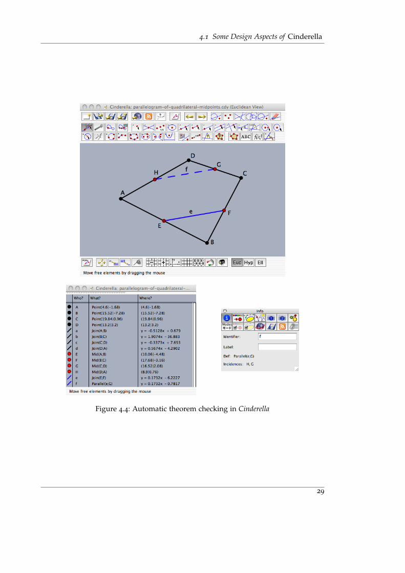
desired result—Cinderella is able to decide whether they are equivalent.As an example, assume we are given an arbitrary quadrilateral ABCD and the
midpoints E, F, G and H of it‘s sides. There is a theorem stating that then EFGH isa parallelogram. This fact is recognized by Cinderella, as shown in the screenshots 4.4.In the left corner, below the Euclidean viewport, we see Cinderella‘s construction textwindow, which, besides the current position of the elements, shows their definition (the“What?” column). Note that the order of elements corresponds to their construction;each object is defined only by preceding objects. In particular, this means that definitionshave to be acyclic; no operation allowed in Cinderella other than dragging inputs withsome degree of freedom can change the currently existing design.
Finally, in the lower right the information about a single element is shown. Here theline f is selected, along with it‘s definition as the parallel to e through G. Cinderellaautomatically detects that f is incident to H, in addition to the trivial incidence with G.
The gathering of this information does not rely on a given set of theorems. Instead,Cinderella randomly generates several possible instances continuously reachable fromthe construction with respect to the definitions of elements. If an incidences is consistent
28
4.1 Some Design Aspects of Cinderella
Figure 4.4: Automatic theorem checking in Cinderella
29

4 Simulation of Kempe Linkages using Cinderella and Xalci
over all these tries, it is reported as proven. The results of the checks are used to someextent to avoid unnecessary duplications of constructions and, thus, saving computationtime.
The number of tests performed is chosen to match an undocumented, but seeminglyvery high probability. Since all calculations in Cinderella are done with floating pointarithmetics, Kortenkamp however has to admit that the theorem checker can be fooledby constructions involving extreme intermediate values.
The combination of continuity guarantees and intrinsic theorem checking allows totake up Abbott et al.’s criticism on Kempe‘s elementary linkages explained in section3.4 from another point of view. The addressed problems of the occurences of additionalconfigurations are automatically avoided by Cinderella, since it‘s continuity modelsimultaneously applies to all elements of the construction.
As long as we build upon a nondegenerate state in the beginning, incidences such asthe parallelity of the bars of the translators remain invariant under arbitrary movements.Thus, even if we don’t define the parallelogram linkage by the geometric primitiveoffered by the system, but position the hinges, say C of figure 3.3, on one of the twointersection points of circles determining the bar lengths, Cinderella will remember thischoice throughout the construction.
4.1.4 CindyScript
An implementation of automated linkage generation would not have been possiblewithout some interface to instruct Cinderella which operations to perform. This is ableby the use of CindyScript, a functional high level language interpreted by Cinderella.Besides common features of any object-oriented programming language it allows tointeractively modify the construction data. For this purpose both a command shell anda script editor are offered; the latter can react on events like user input or redrawing ofthe viewport.
The CindyScript interpreter is also part of Cinderella applets, thus predefined scriptscan also be used in web presentations. In addition, the authors recently added aninterface allowing foreign applets to execute CindyScript commands from the outside.Our implementation almost exclusively uses this way of communication with Cinderella.
This feature still is in the testing stage, and it turned out to have several issues notyet completely eliminated. In particular, Cinderella currently is not able to reliably givefeedback to the outside after execution of an instruction. As a necessary consequence,our implementation controls Cinderella through a blindfold. Since we intendedly do nottry to double the geometric computations and cannot inspect the internal information
30
4.2 Visualization of Implicit Algebraic Curves using Xalci
of Cinderella, we are thus not yet completely able to adapt input parameters such as thedimensions of the linkwork according to the restrictions of the viewport or the givencurve.
4.2 Visualization of Implicit Algebraic Curves using Xalci
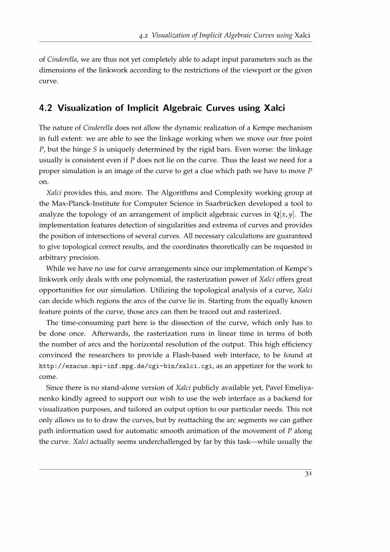
The nature of Cinderella does not allow the dynamic realization of a Kempe mechanismin full extent: we are able to see the linkage working when we move our free pointP, but the hinge S is uniquely determined by the rigid bars. Even worse: the linkageusually is consistent even if P does not lie on the curve. Thus the least we need for aproper simulation is an image of the curve to get a clue which path we have to move Pon.
Xalci provides this, and more. The Algorithms and Complexity working group atthe Max-Planck-Institute for Computer Science in Saarbrucken developed a tool toanalyze the topology of an arrangement of implicit algebraic curves in Q[x, y]. Theimplementation features detection of singularities and extrema of curves and providesthe position of intersections of several curves. All necessary calculations are guaranteedto give topological correct results, and the coordinates theoretically can be requested inarbitrary precision.
While we have no use for curve arrangements since our implementation of Kempe‘slinkwork only deals with one polynomial, the rasterization power of Xalci offers greatopportunities for our simulation. Utilizing the topological analysis of a curve, Xalcican decide which regions the arcs of the curve lie in. Starting from the equally knownfeature points of the curve, those arcs can then be traced out and rasterized.
The time-consuming part here is the dissection of the curve, which only has tobe done once. Afterwards, the rasterization runs in linear time in terms of boththe number of arcs and the horizontal resolution of the output. This high efficiencyconvinced the researchers to provide a Flash-based web interface, to be found athttp://exacus.mpi-inf.mpg.de/cgi-bin/xalci.cgi, as an appetizer for the work tocome.
Since there is no stand-alone version of Xalci publicly available yet, Pavel Emeliya-nenko kindly agreed to support our wish to use the web interface as a backend forvisualization purposes, and tailored an output option to our particular needs. This notonly allows us to to draw the curves, but by reattaching the arc segments we can gatherpath information used for automatic smooth animation of the movement of P alongthe curve. Xalci actually seems underchallenged by far by this task—while usually the
31

4 Simulation of Kempe Linkages using Cinderella and Xalci
correct visualization of implicit curves is considered a very expensive computation,neither Xalci nor the web transport turned out to be a bottleneck in our simulation.
The interface still might be a subject to change during the further developement ofXalci.
4.3 Geometric Primitives in Linkage Simulation
As mentioned in the introductory paragraphs to this chapter, in a DGS like Cinderellayou do not have the possibilities nor the needs to mimic a linkwork in every detail. How-ever, we can simulate all geometric computations performed during the constructionalgorithm presented in section 3.2.
Since arbitrary reals cannot be represented in Cinderella, we demand the inputpolynomial to have rational coefficients, as well as m, n ∈ Q. A quick look on thetransformations done to obtain fm,n from f shows that all coefficents as,t, bs,t and c arerational, too. The reader might ask whether this is really necessary because Cinderellauses floating-point arithmetics, so results will be inexact anyway, and he will havea point there. Approximating arbitrary reals will yield the same precision as ourapproach. But our goal is a theoretically correct implementation, which at least has tofeature correct algorithms, even if they cannot be handled in full extent by the toolsused, and there are lengths of irrational measure (such as π) not constructible withthe primitive operations allowed by any ruler and compass approach regardless of theunderlying implementation.
Our implementation proceeds in the same steps as Kempe‘s description:
0. • We start by establishing the coordinate system by defining points O = (0, 0)and X = (1, 0) at fixed coordinates and draw the unit circle through Xaround O.
P is initialized to an arbitrary starting position within the open set reachableby the bars avoiding the degenerate case where the supporting lines of thebars overlap. Obviously, a preferable choice is some point on the curve; sinceP is free to move anyway, we can safely use the positioning facilities offeredby Cinderella.
• Since m and n are rational numbers, they are constructible, meaning thereare ruler-compass constructions to find a point mX with distance m to Oand m − 1 to X, only depending on O and X.1 The procedure allowing
1A more formal definition of the constructability of x is that x is contained in an iterated algebraic field
32

4.3 Geometric Primitives in Linkage Simulation
to generate mX and nX is presented in step 5 and does not depend onintermediate elements; so we can for now assume to have given points fromwhich we can take the lengths m and n to the origin and draw circles ofradius m around O and n around P.
One of their intersection points is chosen as a possible instance of A1. Joins,i.e. defining a line (achieved by Peaucellier cells in linkages), are primitiveoperations in a DGS as well as the drawing of parallels through given points,so we can determine the point B1 as the intersection of the parallels to OA1
through P and A1P through O.
1. In Cinderella, contrary to deterministic geometry systems, we have to face thesame problems regarding the orientation of the y-axis discussed in section 3.2.Just choosing a third free point will prevent the program to apply it‘s incidencechecking on elements depending on the axis, since the defining third point mightmove later. Thus we have to take any of the two intersections of the unit circleand the y-axis (defined as the perpendicular on OX through O) for Y.
This is just mentioned for the sake of completeness and does not cause anytrouble, because after all the same instruction sequence will always cause thesame result to appear on the screen.
2. We now generate points on the unit circle representing the angles ϕ and θ. Thiscan be done by dividing the distances of A1 and B1 to O by m and n; again, werefer to step 5.
For clearness, in figure 4.5 (a) the points are already assumed to be on the unitcircle. Then to yield a multiple of an angle (θ, corresponding to B1, in the figure)it is sufficient to iteratively draw circles around Bt through Bt−1, starting withB1 and X. There is at most one additional intersection of these circles with theunit circle besides Bt−1; this point gives Bt+1 with angle ]XOBt+1 = (t + 1)θ bycongruence of 4Bt−1OBt and 4BtOBt+1.
If there is no additional intersection, ]Bt−1OBt = π, which is a degenerate casenot induced by boundary constraints other than the position of P, which is
extension of degree two of Q. The field operations +, −, · and ·· are linear operations, which can beachieved by the ruler; additionaly, the constructible numbers are closed under
√·, which corresponds
to the solving of polynomial equations in degree two, or, geometrically, intersections of circles andlines or circles.
All operations but root extraction involved are used and presented throughout this construction; fora more concise treatment of the topic see e.g. [Lab08] or introductory textbooks on algebraic numbertheory.
33
4 Simulation of Kempe Linkages using Cinderella and Xalci
(a) multiplication of angles (b) addition of angles
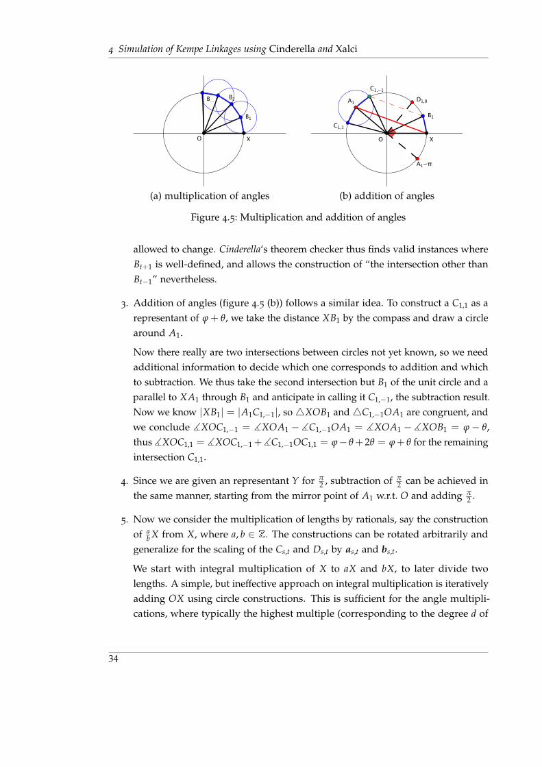
Figure 4.5: Multiplication and addition of angles
allowed to change. Cinderella‘s theorem checker thus finds valid instances whereBt+1 is well-defined, and allows the construction of “the intersection other thanBt−1” nevertheless.
3. Addition of angles (figure 4.5 (b)) follows a similar idea. To construct a C1,1 as arepresentant of ϕ + θ, we take the distance XB1 by the compass and draw a circlearound A1.
Now there really are two intersections between circles not yet known, so we needadditional information to decide which one corresponds to addition and whichto subtraction. We thus take the second intersection but B1 of the unit circle and aparallel to XA1 through B1 and anticipate in calling it C1,−1, the subtraction result.Now we know |XB1| = |A1C1,−1|, so 4XOB1 and 4C1,−1OA1 are congruent, andwe conclude ]XOC1,−1 = ]XOA1 −]C1,−1OA1 = ]XOA1 −]XOB1 = ϕ− θ,thus ]XOC1,1 = ]XOC1,−1 +]C1,−1OC1,1 = ϕ− θ + 2θ = ϕ + θ for the remainingintersection C1,1.
4. Since we are given an representant Y for π2 , subtraction of π
2 can be achieved inthe same manner, starting from the mirror point of A1 w.r.t. O and adding π
2 .
5. Now we consider the multiplication of lengths by rationals, say the constructionof a
b X from X, where a, b ∈ Z. The constructions can be rotated arbitrarily andgeneralize for the scaling of the Cs,t and Ds,t by as,t and bs,t.
We start with integral multiplication of X to aX and bX, to later divide twolengths. A simple, but ineffective approach on integral multiplication is iterativelyadding OX using circle constructions. This is sufficient for the angle multipli-cations, where typically the highest multiple (corresponding to the degree d of
34

4.3 Geometric Primitives in Linkage Simulation
Figure 4.6: Multiplication of lengths
Figure 4.7: Division of lengths by application of the intercept theorem
the polynomial f ) is rather low; however, this usually is not the case for thecoefficients.
Instead, we first construct all powers of two 2iX using circles in correspondingsizes as shown in figure 4.6. Then we add the required powers to get the finalresult (5X here). This is done using the depicted parallels construction, equivalentto the translator linkage, which moves OX (or some arbitrary multiple) to 4X,yielding 5X. Thus we achieve a reduction of the construction complexity fromO(a) to O(log a), compared to the trivial solution.
Division is allowed by the intercept theorem, as depicted in figure 4.7. Startingfrom aX and bX, we join the divisor bX with Y. The intersection S of the parallelthough the dividend aX with the y-axis satisfies a
b = |OaX||ObX| = |OS|
|OY| , thus S = ab Y.
Rotation back to the x-axis yields ab X.
Note that the orientation of the y-axis matters for none of the constructionsmentioned above, so we are free to use −Y instead if we are not yet able todecide which point corresponds to the angle rotated by 90 degrees clockwise. Fora length not coinciding with the x-axis, we imagine any of the two intersections
35
4 Simulation of Kempe Linkages using Cinderella and Xalci
of a perpendicular through O and the unit circle as a local Y. This is especiallyimportant for getting the position of the points A1 and B1 on the unit circle instep 1.
6. Finally, the easiest step throughout the simulation is the summation of all oc-curing terms. Since we do not need to care about fixed bar lengths—those areautomatically adapted by the DGS—we can employ the simple parallelogramconstruction of figure 2.4 (a).
4.4 Presentation of Our Simulation of Kempe Linkages
We want to complete this chapter with a presentation of our implementation, accessibleto anyone interested at http://www.math.uni-sb.de/ag/schreyer/Kempe-Linkage/.
Our solution is written in Java and designed as an applet, a decision made to easethe communication with Cinderella. The exact rational arithmetics needed for thetransformation of f to fm,n are provided by the free open source JScience library [JSc].The complete application amounts to approximately 6500 lines of code, including theXalci interface; sources are available on request.
4.4.1 The User Interface
Figure 4.8 shows the user interface of our program, giving an overview of the function-ality.
Using Xalci‘s rasterization of the curve, we are able to approximate coordinates ofa random point P on the curve within the current viewport. Consequently, we offerautomatical adaption of the bar length s.t. P is reached without forcing the initialparallelogram to an excessive elongation.
Up to now, there is no support for shifting the viewport of a Cinderella appletfrom outside, nor can we obtain the coordinates of the shown area. As a necessaryconsequence, we made the obvious decision to fix the view around the origin of thecoordinate system. Therefore we offer the translation of the straight line S moves on tothe y-axis, a part of which is always visible. For a minimum of convenience, we areable to allow arbitrary zooming.
Due to the complexity of the construction the output tends to become extremelymessy; to face this inevitable problem, several intermediate construction steps can behidden from the user. The defaults are reasonably chosen to get an idea of the dynamicsof the construction without to much clutter (figure 4.9).
36

4.4 Presentation of Our Simulation of Kempe Linkages
Figure 4.8: The graphical user interface of our implementation
For a deeper insight to the construction, we log all steps done throughout the con-struction in the CindyScript instruction format. Thus the user can redo the operationsin a stand-alone instance of Cinderella and examine the simulation in every detail,although without our interface to Xalci. For short requests, the user can also use aCindyScript command line inside our application.
4.4.2 Animations
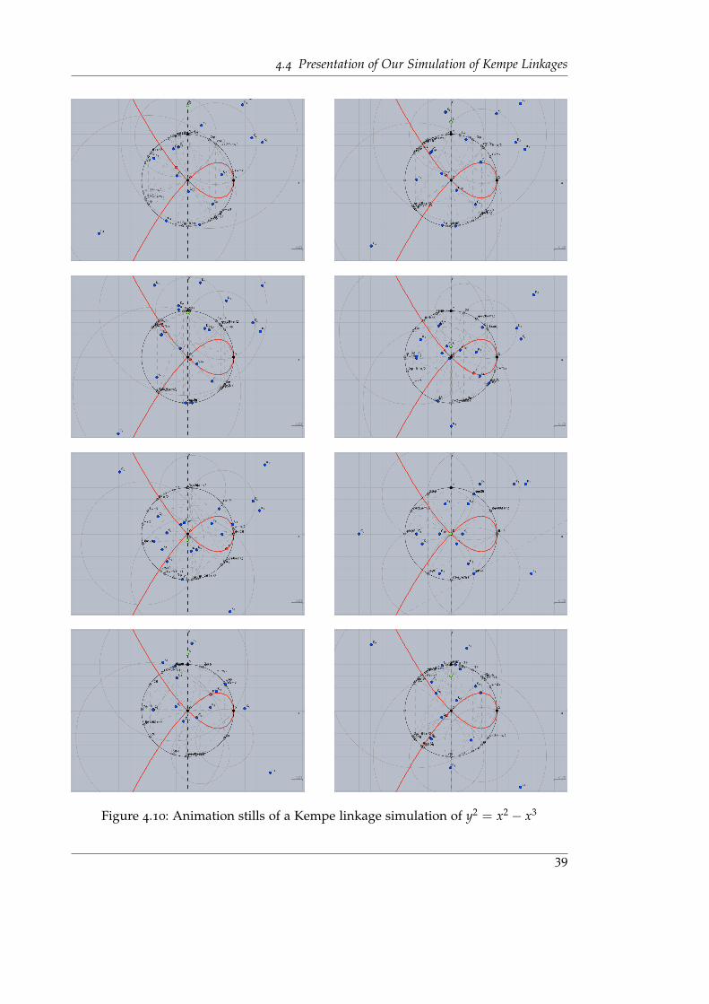
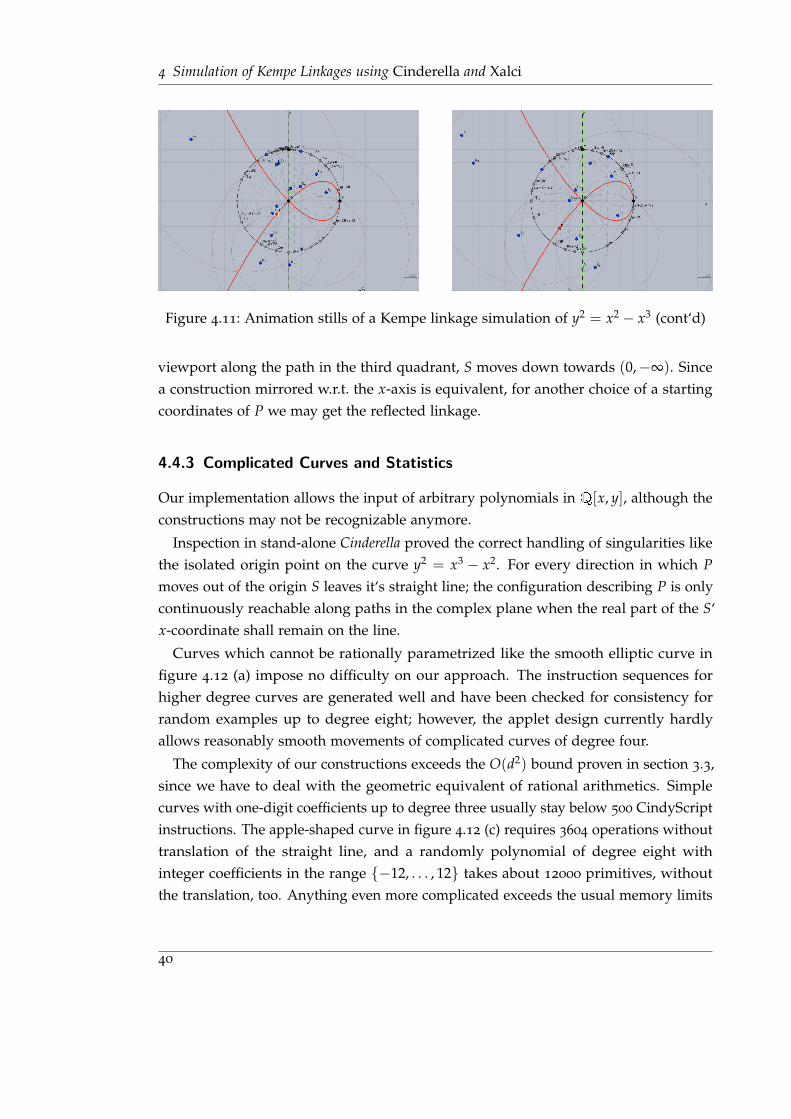
Sadly, a printout cannot express the dynamic nature of an animation very well. At leastwe can give some screenshots throughout a simulation (figures 4.10 and 4.11). Wetrace the motion of S while P moves along the curve C = V(y2 + x3 − x2); our setupuses m = n = 1. In the trigonometric form of the polynomial, no offset by constantterms occurs, so the line S stays on is the y-axis.
When P enters the viewport into the second quadrant, S comes along from above.Through the self-intersection of the curve in the origin, S continuously passes (0, 1),to oscillate around the origin while P describes the loop of C. When P leaves the
37

4 Simulation of Kempe Linkages using Cinderella and Xalci
Figure 4.9: A view of all intermediate elements of a construction, in contrast to a moretidy version.
38
4.4 Presentation of Our Simulation of Kempe Linkages
Figure 4.10: Animation stills of a Kempe linkage simulation of y2 = x2 − x3
39
4 Simulation of Kempe Linkages using Cinderella and Xalci
Figure 4.11: Animation stills of a Kempe linkage simulation of y2 = x2 − x3 (cont‘d)
viewport along the path in the third quadrant, S moves down towards (0,−∞). Sincea construction mirrored w.r.t. the x-axis is equivalent, for another choice of a startingcoordinates of P we may get the reflected linkage.
4.4.3 Complicated Curves and Statistics
Our implementation allows the input of arbitrary polynomials in Q[x, y], although theconstructions may not be recognizable anymore.
Inspection in stand-alone Cinderella proved the correct handling of singularities likethe isolated origin point on the curve y2 = x3 − x2. For every direction in which Pmoves out of the origin S leaves it‘s straight line; the configuration describing P is onlycontinuously reachable along paths in the complex plane when the real part of the S‘x-coordinate shall remain on the line.
Curves which cannot be rationally parametrized like the smooth elliptic curve infigure 4.12 (a) impose no difficulty on our approach. The instruction sequences forhigher degree curves are generated well and have been checked for consistency forrandom examples up to degree eight; however, the applet design currently hardlyallows reasonably smooth movements of complicated curves of degree four.
The complexity of our constructions exceeds the O(d2) bound proven in section 3.3,since we have to deal with the geometric equivalent of rational arithmetics. Simplecurves with one-digit coefficients up to degree three usually stay below 500 CindyScriptinstructions. The apple-shaped curve in figure 4.12 (c) requires 3604 operations withouttranslation of the straight line, and a randomly polynomial of degree eight withinteger coefficients in the range {−12, . . . , 12} takes about 12000 primitives, withoutthe translation, too. Anything even more complicated exceeds the usual memory limits
40
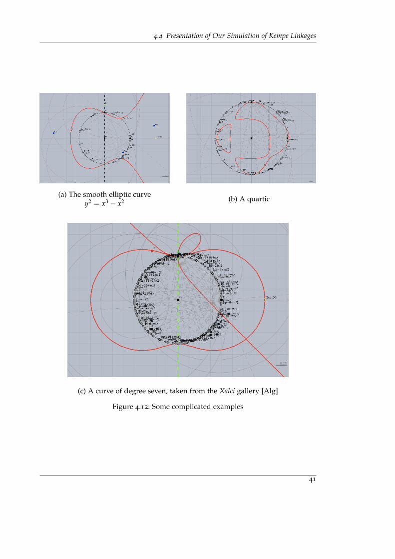
4.4 Presentation of Our Simulation of Kempe Linkages
(a) The smooth elliptic curvey2 = x3 − x2 (b) A quartic
(c) A curve of degree seven, taken from the Xalci gallery [Alg]
Figure 4.12: Some complicated examples
41

4 Simulation of Kempe Linkages using Cinderella and Xalci
of Java‘s virtual machine; we do not have to mention that the graphical output takes fartoo long to be of more than theoretical interest.
4.5 Conclusion
While we have been able to give a proof-of-concept implementation, we have to admitthat the examination of the results is no fun so far. The interface to Cinderella, whileproviding a comprehensive choice of geometric operations, is just not designed forkiller applications like Kempe linkages. However, there is reason to hope that ourimplementation will motivate others to use the said interface, and thus invite theCinderella authors to refine it. Even if our project will not benefit, others certainly will.
Still, no dynamical geometry system existing by now allows to perform the taskof moving S to trace out the curve, which is the more interesting direction of thetranslation. Currently we are not aware of any solution to this. Gao et al. mention theirsoftware Geometry Expert to perform this task, but apparently it is lost, and there is nointerest in reanimating it.
Finally, further investigations can be done in the field of lower bounds of exactlinkage complexity for particular classes of curves, which still is a widely unchartedterrain.
42

Bibliography
[ABD08] Timothy Good Abbott, Reid W. Barton, and Erik D. Demaine. Generaliza-tions of Kempe‘s Universality Theorem. Master’s thesis, MassachusettsInstitute of Technology, June 2008.
[Alg] Algorithms and Complexity working group at Max-Planck-Institute forComputer Science. Xalci. http://exacus.mpi-inf.mpg.de/cgi-bin/xalci.cgi.
[Eme07] Pavel Emeliyanenko. Visualization of Points and Segments of Real AlgebraicPlane Curves. Master’s thesis, Saarland University, Saarbrucken, 2007.
[Gaw03] Thomas Gawlick. Uber die Machtigkeit dynamischer Konstruktionenmit verschiedenen Werkzeugen. http://www.uni-bielefeld.de/idm/
service/bib_dok/publikationen/occpap.html, February 2003.
[GZCG02] Xiao-Shan Gao, Chang-Cai Zhu, Shang-Ching Chou, and Jian-Xin Ge. Auto-mated Generation of Kempe Linkages for Algebraic Curves and Surfaces.In Mechanism and Machine Theory, volume 36, pages 1019–1033, 2002.
[JSc] JScience. http://jscience.org/.
[Kem76] Alfred Bray Kempe. On a General Method of describing Plane Curves of thenth degree by Linkwork. In Proc. of London Mathematical Society, volume 7,pages 213–216, 1876.
[Kem77] Alfred Bray Kempe. How to Draw a Straight Line – A lecture on linkages.Nature Series. Macmillan and Co., London, 1877.
[Ker06] Michael Kerber. Analysis of Real Algebraic Plane Curves. Master’s thesis,Saarland University, Saarbrucken, 2006.
[Kin98] Henry C. King. Configuration Spaces of Linkages in Rn.arXiv.org:math/9811138, 1998.
[Kor99] Ulrich Kortenkamp. Foundations of Dynamic Geometry. PhD thesis, SwissFederal Institute of Technology, Zurich, 1999.
43

Bibliography
[KRG] Ulrich Kortenkamp and Jurgen Richter-Gebert. Cinderella.http://www.cinderella.de/.
[Lab08] Oliver Labs. Dynamische Geometrie: Grundlagen und Anwendungen.http://www.math.uni-sb.de/ag/schreyer/, 2007–2008.
44