Automated Estimation of Vector Error Correction Models�

Zhipeng Liao y Peter C. B. Phillips z

First Version: June, 2010; This Version: November 2013

Abstract

Model selection and associated issues of post-model selection inference present well known

challenges in empirical econometric research. These modeling issues are manifest in all applied

work but they are particularly acute in multivariate time series settings such as cointegrated

systems where multiple interconnected decisions can materially a¤ect the form of the model

and its interpretation. In cointegrated system modeling, empirical estimation typically proceeds

in a stepwise manner that involves the determination of cointegrating rank and autoregressive

lag order in a reduced rank vector autoregression followed by estimation and inference. This

paper proposes an automated approach to cointegrated system modeling that uses adaptive

shrinkage techniques to estimate vector error correction models with unknown cointegrating

rank structure and unknown transient lag dynamic order. These methods enable simultaneous

order estimation of the cointegrating rank and autoregressive order in conjunction with oracle-

like e¢ cient estimation of the cointegrating matrix and transient dynamics. As such they o¤er

considerable advantages to the practitioner as an automated approach to the estimation of

cointegrated systems. The paper develops the new methods, derives their limit theory, discusses

implementation, reports simulations and presents an empirical illustration with macroeconomic

aggregates.

Keywords: Adaptive shrinkage; Automation; Cointegrating rank; Lasso regression; Oracle e¢ -

ciency; Transient dynamics; Vector error correction.

JEL classi�cation: C22

�Comments from two referees and the Co-Editor helped guide the revision of this paper and are gratefully ac-knowledged.

yDepartment of Economics, UC Los Angeles, 8379 Bunche Hall, Mail Stop: 147703, Los Angeles, CA 90095.Email: zhipeng.liao@econ.ucla.edu

zYale University, University of Auckland, University of Southampton and Singapore Management University.Support from the NSF under Grant Nos. SES 09-56687 and SES 12-58258 is gratefully acknowledged. Email:peter.phillips@yale.edu

1

1 Introduction

Cointegrated system modeling is now one of the main workhorses in empirical time series research.

Much of this empirical research makes use of vector error correction (VEC) formulations. While

there is often some prior information concerning the number of cointegrating vectors, most practical

work involves (at least con�rmatory) pre-testing to determine the cointegrating rank of the system

as well as the lag order in the autoregressive component that embodies the transient dynamics.

These order selection decisions can be made by sequential likelihood ratio tests (e.g. Johansen,

1988, for rank determination) or the application of suitable information criteria (Phillips, 1996).

Both approaches are popular in empirical research.

Information criteria o¤er certain advantages such as joint determination of the cointegrating

rank and autoregressive order, consistent estimation of both order parameters (Chao and Phillips,

1999; Athanasopoulos et al., 2011), robustness to heterogeneity in the errors, and the convenience

and generality of semi-parametric estimation in cases where the focus is simply the cointegrating

rank (Cheng and Phillips, 2010, 2012). Sequential testing procedures have recent enhancements

including bootstrap modi�cations to improve test performance and under certain conditions provide

consistent order estimation by adaptation if test size is driven to zero as the sample size expands

to in�nity. However, these adaptive methods have not been systematically investigated in the VEC

framework and there is little research on rate control and testing order, and no asymptotics for

such adaptive procedures to o¤er guidance for empirical implementation. More importantly in

the VEC setting, sequential tests involve di¤erent test statistics for lags and cointegrating rank,

and model selection is inevitably unstable in the sense that di¤erent models may be selected when

di¤erent sequential orders are used. Moreover, general to speci�c and speci�c to general testing

algorithms encounter obstacles to consistent model selection even when test size is driven to zero

(see Section 9 for an example). Finally, while they are appealing to practitioners, all of these

methods are nonetheless subject to pre-test bias and post model selection inferential problems

(Leeb and Pötscher, 2005).

The present paper explores a di¤erent approach. The goal is to liberate the empirical researcher

from some of the di¢ culties of sequential testing and order estimation procedures in inference

about cointegrated systems and in policy work that relies on associated impulse responses. The

ideas originate in recent work on sparse system estimation using shrinkage techniques such as Lasso

and bridge regression. These procedures utilize penalized least squares criteria in regression that

can succeed, at least asymptotically, in selecting the correct regressors in a linear regression frame-

work while consistently estimating the non-zero regression coe¢ cients. Caner and Knight (2013)

�rst showed how this type of estimator may be used in a univariate autoregressive model with a

2

potential unit root. While apparently e¤ective asymptotically these procedures do not avoid post

model selection inference issues in �nite samples because the estimators implicitly carry e¤ects from

the implementation of shrinkage which can result in bias, multimodal distributions and di¢ culty

discriminating local alternatives that can lead to unbounded risk (Leeb and Pötscher, 2008). On

the other hand, the methods do radically simplify empirical research with large dimensional sys-

tems where order parameters must be chosen and sparsity is expected. When data-based tuning

parameter selection is employed, the methods also enable automated implementation making them

convenient for empirical practice.

One of the contributions of this paper is to develop new adaptive versions of shrinkage methods

that apply in vector error correction modeling which by their nature involve reduced rank coe¢ cient

matrices and order parameters for lag polynomials and trend speci�cations. The implementation

of these methods in this econometric setting is by no means immediate. In particular, multivariate

models with some unit roots and cointegration involve dimension reductions and nonlinear restric-

tions which present new di¢ culties of both formulation and asymptotics in the Lasso framework

that go beyond existing work in the statistics literature such as Yuan et al (2007). The present pa-

per contributes to the Lasso and econometric literatures by providing a new penalty function that

handles these complications, developing a rigorous limit theory of order selection and estimation

for this multivariate nonlinear nonstationary setting, and devising a straightforward method of im-

plementation that is well suited to empirical econometric research. When reduced to the univariate

case, our results cover the methodology and implicit unit root test procedure suggested in Caner

and Knight (2013) and extend their univariate results to cases where there is misspeci�cation in

the transient dynamics.

The paper designs a mechanism of estimation and selection that works through the eigenvalues of

the levels coe¢ cient matrix and the coe¢ cient matrices of the transient dynamic components. This

formulation is necessary because of the nonlinearities involved in potential reduced rank structures

and the interdependence of decision making concerning the form of the transient dynamics and

the cointegrating rank structure. The resulting methods apply in quite general vector systems

with unknown cointegrating rank structure and unknown lag dynamics. They permit simultaneous

order estimation of the cointegrating rank and autoregressive order in conjunction with oracle-

like e¢ cient estimation of the cointegrating matrix and transient dynamics. As such they o¤er

considerable advantages to the practitioner. In e¤ect, it becomes unnecessary to implement pre-

testing procedures because the empirical results reveal all of the order parameters as a consequence

of the �tting procedure.

A novel contribution of the paper in this nonlinear setting where eigenvalues play a key role is the

3

use of a penalty which is a simple convex function of the coe¢ cient matrix. The new penalty makes

penalized estimation stable and accurate, facilitates the limit theory, and simpli�es implementation

because existing code for grouped L-1 penalized estimation can be used for computation. All the

theoretical results are rigorously derived in a general nonstationary set-up that allows for unit

roots, cointegration and transient dynamics, which combines with the new penalty formulation

to complement recent asymptotic theory for Lasso estimation in stationary vector autoregressive

(VAR) models (Song and Bickel, 2009; Kock and Callot, 2012) and multivariate regression (Yuan

et al, 2007; Peng et al., 2010).

The paper is organized as follows. Section 2 lays out the model and assumptions and shows how

to implement adaptive shrinkage methods in VEC systems. Section 3 considers a simpli�ed �rst

order version of the vector error correction model (VECM) without lagged di¤erences which reveals

the approach to cointegrating rank selection and develops key elements in the limit theory. Here

we show that the cointegrating rank ro is identi�ed by the number of zero eigenvalues of �o and

the latter is consistently recovered by suitably designed shrinkage estimation. Section 4 extends

this system and its asymptotics to the general case of cointegrated systems with weakly dependent

errors. Here it is demonstrated that the cointegration rank ro can be consistently selected despite

the fact that �o itself may not be consistently estimable. Section 5 deals with the practically

important case of a general VEC system driven by independent identically distributed (iid) shocks,

where shrinkage estimation simultaneously performs consistent lag selection, cointegrating rank

selection, and optimal estimation of the system coe¢ cients. Section 6 considers adaptive selection

of the tuning parameter and Section 7 reports some simulation �ndings. Section 8 applies our

method to an empirical example. Section 9 concludes and outlines some useful extensions of the

methods and limit theory to other models. Proofs are given in the Appendix. A Supplement to

the paper (Liao and Phillips, 2013) provides supporting lemmas and technical results.

Notation is standard. For vector-valued, zero mean, covariance stationary stochastic processes

fatgt�1 and fbtgt�1, �ab(h) = E[atb0t+h] and �ab =P1h=0�ab(h) denote the lag h autocovariance

matrix and one-sided long-run covariance matrix. Moreover, we use �ab for �ab(0) and �n;ab =

n�1Pnt=1 atb

0t as the corresponding sample average. The notation k�k denotes the Euclidean norm

and jAj is the determinant of a square matrix A. A0 refers to the transpose of any matrix A andkAkB � jjA0BAjj for any conformable matrices A and B. Ik and 0l are used to denote k � kidentity matrix and l� l zero matrices respectively. The symbolism A � B means that A is de�nedas B; the expression an = op(bn) signi�es that Pr (jan=bnj � �)! 0 for all � > 0 as n go to in�nity;

and an = Op(bn) when Pr (jan=bnj �M) ! 0 as n and M go to in�nity. As usual, "!p" and

"!d" imply convergence in probability and convergence in distribution, respectively. Following

4

standard convention we frequently write integrals of stochastic processes (V;W ) over [0; 1] such as�R 10 V (r) dW (r)0 ;

R 10 V (r)V (r)

0 dr�in the simple form

�RV dW 0;

RV V 0

�.

2 Vector Error Correction and Adaptive Shrinkage

Throughout this paper we consider the following parametric VEC representation of a cointegrated

system

�Yt = �oYt�1 +

pXj=1

Bo;j�Yt�j + ut; (2.1)

where �Yt = Yt � Yt�1; Yt is an m-dimensional vector-valued time series, �o = �o�0o has rank

0 � ro � m, Bo;j (j = 1; :::; p) are m �m (transient) coe¢ cient matrices, ut is an m-vector error

term with mean zero and nonsingular covariance matrix �uu, m and p are �xed positive integers.

The rank ro of �o is an order parameter measuring the cointegrating rank or the number of (long

run) cointegrating relations in the system. The index set of non zero matrices Bo;j (j = 1; :::; p) is

a second order parameter, characterizing the transient dynamics in the system.

As �o = �o�0o has rank ro, we can choose �o and �o to be m�ro matrices with full rank. Whenro = 0, we simply take �o = 0. Let �o;? and �o;? be the matrix orthogonal complements of �o

and �o, i.e. �o;? and �o;? are full rank m� (m� ro) matrices satisfying �0o;?�o = 0(m�ro)�m and�0o;?�o = 0(m�ro)�m respectively. Without loss of generality, assume that �0o;?�o;? = Im�ro and

�0o;?�o;? = Im�ro .1

Suppose �o 6= 0 and de�ne Q = [�o; �o?]0 : In view of the well known relation (e.g., Johansen,1995)

�o(�0o�o)

�1�0o + �o;?(�0o;?�o;?)

�1�0o;? = Im; (2.2)

it follows that Q�1 =h�o(�

0o�o)

�1; �o;?(�0o;?�o;?)

�1i,

Q�o =

24 �0o�o�0o0

35 and Q�oQ�1 =

24 �0o�o 0

0 0

35 : (2.3)

Under Assumption RR in Section 3, �0o�o is an invertible matrix and hence the matrix �0o�o�

0o has

full rank. Cointegrating rank is the number ro of non zero eigenvalues of �o or the nonzero row

vector count of Q�o. When �o = 0, then the result holds trivially with ro = 0 and �o;? = Im.

The matrices �o? and �o;? are composed of normalized left and right eigenvectors, respectively,

1When m � ro > 1, the normalizations �0o;?�o;? = Im�ro and �0o;?�o;? = Im�ro are not su¢ cient to ensure

the uniqueness of �o;? and �o;?. In the paper, we only need the existence of normalized �o;? and �o;? such that�0o;?�o = 0 and �

0o;?�o = 0.

5

corresponding to the zero eigenvalues in �o.

Conventional methods of estimation of (2.1) include reduced rank regression or maximum like-

lihood based on the assumption of Gaussian ut and a Gaussian likelihood. This approach relies on

known ro and known transient dynamics structure, so implementation requires preliminary order

parameter estimation. The system can also be estimated by unrestricted fully modi�ed vector

autoregression (Phillips, 1995), which leads to consistent estimation of the unit roots in (2.1), the

cointegrating vectors and the transient dynamics. This method does not require knowledge of ro

but does require knowledge of the transient dynamics structure. In addition, a semiparametric ap-

proach can be adopted in which ro is estimated semiparametrically by order selection as in Cheng

and Phillips (2010, 2012) followed by fully modi�ed least squares regression to estimate the cointe-

grating matrix. That approach achieves asymptotically e¢ cient estimation of the long run relations

(under Gaussianity) but does not estimate the transient relations.

The present paper explores direct estimation of the parameters of (2.1) by Lasso-type regression.

The resulting estimator is a shrinkage estimator that takes account of potential degeneracies in the

system involving both long run reduced rank structures and transient dynamics. Speci�cally, the

least squares (LS) shrinkage estimator of (�o; Bo) where Bo = (Bo;1; :::; Bo;p) is de�ned as

(b�n; bBn) = argmin�;B1;:::;Bp2Rm�m

(nXt=1

�Yt ��Yt�1 �Xj�p

Bj�Yt�j

2+n

pXj=1

�b;j;n kBjk+ nmXk=1

�r;k;n k�n;k(�)k

9=; (2.4)

where �b;j;n and �r;k;n (j = 1; :::; p and k = 1; :::;m) are tuning parameters that directly control the

penalization, �n;k(�) is the k-th row vector of Qn�, and Qn denotes the normalized left eigenvector

matrix of eigenvalues of b�1st. The matrix b�1st is some �rst step (e.g., OLS) estimate of �o. Thepenalty function on the coe¢ cients Bj (j = 1; :::; p) of the lagged di¤erences is called a group Lasso

penalty (see, Yuan and Lin, 2006). On the other hand, the penalty function on � is di¤erent from

the group Lasso, because it works on the rows of the adaptively transformed matrix Qn�, not the

rows (or any deterministic functions such as eigenvalues) of � directly.2

Given the tuning parameters, this procedure delivers a one step estimator of the model (2.1) with

an implied estimate of the cointegrating rank (based on the number of non-zero rows of Qnb�n) and2The tranform of the matrix � is important for rank selection because, by virtue of the consistency of the �rst

step estimator b�1st, Qn�o has (and only has) m�ro rows which are asymptotically non zero. Note that the fact thata matrix � does not have full rank does not necessarily mean that any element in � should be zero. Hence penalizedLS regression in (2.4) with a group Lasso penalty on � does not deliver any implication for rank selection in generalcase.

6

an implied estimate of the transient dynamic structure (that is, Bo;j in Bo with kBo;jk = 0 for j =1; :::; p) based on the �tted value bBn. It is therefore well suited to empirical implementation whereinformation is limited concerning model speci�cation. By de�nition, the penalized LS estimate

is invariant to permutation of the lag di¤erences, which implies that the rank and lag di¤erences

selected in the penalized LS estimation are stable regardless the potential structure of the true

model. This feature is a particular advantage of Lasso-type model selection methods over traditional

sequential testing procedures which typically work from general to speci�c formulations.

A novel contribution of this paper is that it provides an adaptive penalty function f(�) =mPk=1

�r;k;n k�n;k(�)k, which enables penalized LS estimation in (2.4) to perform rank selection.3 Im-portantly, this penalty function di¤ers from those proposed in the statistics literature for dimension

reduction in multivariate regression with iid data. For example, Peng et al (2009) assume that the

coe¢ cient matrix has many zero components and suggest dimension reduction by penalizing the

estimates of the components in the coe¢ cient matrix with L-1 and L-2 penalty functions. Yuan

et al (2007) propose to penalize the singular values of the estimate of the coe¢ cient matrix with

an L-1 penalty to achieve dimension reduction. While this approach is intuitive and the idea of

working through the eigenvalues of � was used independently in our own earlier work, Yuan et

al (2007) provide theory only under an orthonormal regressor design, which is unrealistic in VEC

structures with nonstationary data4.

Let �0(�o) = [�01(�o); :::;�0m(�o)] denote the row vectors of Q�o. When futgt�1 is iid or a

martingale di¤erence sequence, the LS estimators (b�1st; bB1st) of (�o; Bo) are well known to beconsistent. The eigenvalues and corresponding eigenspace of �o can also be consistently estimated.

Thus it seems intuitively clear that some form of adaptive penalization can be devised to consistently

distinguish the zero and nonzero components in Bo and �(�o).5 We show that the shrinkage LS

estimator de�ned in (2.4) enjoys these oracle-like properties, in the sense that the zero components

in Bo and �(�o) are estimated as zeros with probability approaching 1 (w.p.a.1). Thus, �o and the

non-zero elements in Bo are estimated as if the form of the true model were known and inferences3The new penalty is de�ned as a function on Rm�m, i.e. on the square matrix �. While this formulation is

relevant in the present setting, it is clear that the approach can be trivially extended to the general case with anymatrix.

4As indicated, the idea in Yuan et al.(2007) is related to the original approach pursued in an earlier version (2010)of the present paper. In that version, we showed that when adding the L-1 penalty on the eigenvalues to the LScriterion, the m�ro smallest eigenvalues of the penalized LS estimate of the cointegration matrix �o have convergencerate faster than n�1. This result has implications for e¢ cient estimation of the VECM when the true model is nested.But it does not necessarily imply model selection because selection requires that zero eigenvalues be estimated aszeros with positive probability. That is a challenging problem due to the highly nonlinear relation between �o andits eigenvalues. The approach pursued in the present paper is far simpler, enhancing implementation and leadingdirectly to the required asymptotic result.

5The adaptive penalization means that the penalization on the estimators of zero components (e.g., zero matricesBo;j) is large, while the penalization on the estimators of non zero components (e.g., non zero matrices Bo;j) is small.

7

can be conducted as if we knew the true cointegration rank ro.

If the transient behavior of (2.1) is misspeci�ed and (for some given lag order p) the error

process futgt�1 is weakly dependent and ro > 0, then consistent estimators of the full matrix

(�o; Bo) are typically unavailable without further assumptions. However, them�ro zero eigenvaluesof �o can still be consistently estimated with an order n convergence rate, while the remaining

eigenvalues of �o are estimated with asymptotic bias at apn convergence rate. The di¤erent

convergence rates of the eigenvalues are important, because when the non-zero eigenvalues of �o

are occasionally (asymptotically) estimated as zeros, the di¤erent convergence rates are useful in

consistently distinguishing the zero eigenvalues from the biasedly estimated non-zero eigenvalues

of �o. Speci�cally, we show that if the estimator of some non-zero eigenvalue of �o has probability

limit zero under misspeci�cation of the lag order, then this estimator will converge in probability

to zero at the ratepn, while estimates of the zero eigenvalues of �o all have convergence rate n.

Hence the tuning parameters f�r;k;ngmk=1 can be constructed in the way such that the adaptivepenalties associated with estimates of zero eigenvalues of �o will diverge to in�nity at a rate faster

than those of estimates of the nonzero eigenvalues of �o, even though the latter also converge

to zero in probability. As we have prior knowledge about these di¤erent divergence rates in a

potentially cointegrated system, we can impose explicit conditions on the convergence rate of the

tuning parameters f�r;k;ngmk=1 to ensure that only ro rows of Qnb�n are adaptively shrunk to zerow.p.a.1.

For the empirical implementation of our approach, we provide data-driven procedures for se-

lecting the tuning parameter of the penalty function in �nite samples. For practical purposes our

method is executed in the following steps, which are explained and demonstrated in detail as the

paper progresses.

(1) After preliminary LS estimation of the system, perform a �rst step GLS shrinkage estimation

with adaptive Lasso (c.f. Zou, 2006) type of tuning parameters

�r;k;n =2 log(n)

njj�k(b�1st)jj�2 and �b;j;n = 2m2 log(n)

njj bBj;1stjj�2

for k = 1; :::;m and j = 1; :::; p, where jj�k(�)jj denotes the k-th largest modulus of the eigenvaluesf�k (�)gmk=1 of the matrix � 6 and bBj;1st is some �rst step (OLS) estimates of Bo;j (j = 1; :::; p).

(2) Construct adaptive tuning parameters using the �rst step GLS shrinkage estimates and the

formulas in (6.10) and (6.11). Using the adaptive tuning parameters, obtain the GLS shrinkage

6Throughout this chapter, for any m �m matrix �, we order the eigenvalues of � in decreasing order by theirmodulus, i.e. k�1 (�)k � k�2 (�)k � ::: � k�m (�)k. When there is a pair of complex conjugate eigenvalues, we orderthe one with a positive imaginary part before the other.

8

estimator (b�g;n; bBg;n) of (�o; Bo) - see (5.12). The cointegration rank selected by the shrinkagemethod is implied by the rank of the shrinkage estimator b�g;n and the lagged di¤erences selectedby the shrinkage method are implied by the nonzero matrices in bBg;n.

(3) The GLS shrinkage estimator contains shrinkage bias introduced by the penalty on the

nonzero eigenvalues of b�g;n and nonzero matrices in bBg;n. To remove this bias, run a reduced rankregression based on the cointegration rank and the model selected in the GLS shrinkage estimation

in step (2).

3 First Order VECM Estimation

This section considers the following simpli�ed �rst order version of (2.1),

�Yt = �oYt�1 + ut = �o�0oYt�1 + ut: (3.1)

The model contains no deterministic trend and no lagged di¤erences. Our focus in this simpli�ed

system is to outline the approach to cointegrating rank selection and develop key elements in the

limit theory, showing consistency in rank selection and reduced rank coe¢ cient matrix estimation.

The theory is extended in subsequent sections to models of the form (2.1).

We start with the following condition on the innovation ut.

Assumption 3.1 (WN) futgt�1 is an m-dimensional iid process with zero mean and nonsingularcovariance matrix u.

Assumption 3.1 ensures that the full parameter matrix �o is consistently estimable in this

simpli�ed system. Under Assumption 3.1, partial sums of ut satisfy the functional law

n�12

[n�]Xt=1

ut !d Bu(�); (3.2)

where Bu(�) is a vector of Brownian motion with variance matrix u. With no material changesin what follows, the iid condition in WN could be weakened to a martingale di¤erence sequence

condition provided the functional law (3.2) still holds together with some related weak convergence

results needed for the limit theory. Cheng and Phillips (2012) developed such a limit theory while

exploring the properties of model selection methods based on information criteria but did not

consider penalized regression approaches.

9

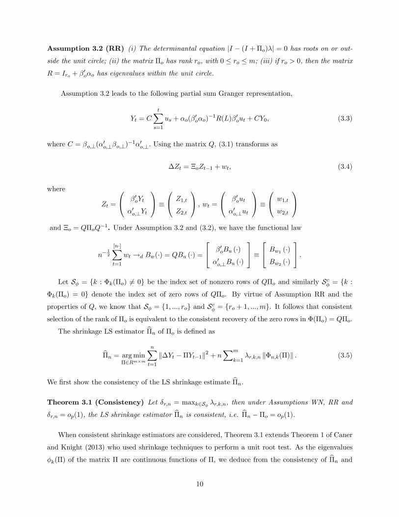
Assumption 3.2 (RR) (i) The determinantal equation jI � (I +�o)�j = 0 has roots on or out-side the unit circle; (ii) the matrix �o has rank ro, with 0 � ro � m; (iii) if ro > 0, then the matrixR = Iro + �

0o�o has eigenvalues within the unit circle.

Assumption 3.2 leads to the following partial sum Granger representation,

Yt = C

tXs=1

us + �o(�0o�o)

�1R(L)�0out + CY0; (3.3)

where C = �o;?(�0o;?�o;?)

�1�0o;?. Using the matrix Q, (3.1) transforms as

�Zt = �oZt�1 + wt; (3.4)

where

Zt =

0@ �0oYt

�0o;?Yt

1A �

0@ Z1;t

Z2;t

1A ; wt =0@ �0out

�0o;?ut

1A �

0@ w1;t

w2;t

1Aand �o = Q�oQ�1. Under Assumption 3.2 and (3.2), we have the functional law

n�12

[n�]Xt=1

wt !d Bw(�) = QBu (�) =

24 �0oBu (�)�0o;?Bu (�)

35 �24 Bw1 (�)Bw2 (�)

35 :Let S� = fk : �k(�o) 6= 0g be the index set of nonzero rows of Q�o and similarly Sc� = fk :

�k(�o) = 0g denote the index set of zero rows of Q�o. By virtue of Assumption RR and the

properties of Q, we know that S� = f1; :::; rog and Sc� = fro + 1; :::;mg. It follows that consistentselection of the rank of �o is equivalent to the consistent recovery of the zero rows in �(�o) = Q�o.

The shrinkage LS estimator b�n of �o is de�ned asb�n = argmin

�2Rm�m

nXt=1

k�Yt ��Yt�1k2 + nXm

k=1�r;k;n k�n;k(�)k : (3.5)

We �rst show the consistency of the LS shrinkage estimate b�n.Theorem 3.1 (Consistency) Let �r;n = maxk2S� �r;k;n, then under Assumptions WN, RR and

�r;n = op(1), the LS shrinkage estimator b�n is consistent, i.e. b�n ��o = op(1).When consistent shrinkage estimators are considered, Theorem 3.1 extends Theorem 1 of Caner

and Knight (2013) who used shrinkage techniques to perform a unit root test. As the eigenvalues

�k(�) of the matrix � are continuous functions of �, we deduce from the consistency of b�n and10

continuous mapping that �k(b�n) !p �k(�o) for all k = 1; :::;m. Theorem 3.1 implies that the

nonzero eigenvalues of �o are estimated as non-zeros, which means that the rank of �o will not be

under-selected. However, consistency of the estimates of the non-zero eigenvalues is not necessary

for consistent cointegration rank selection. In that case what is essential is that the probability

limits of the estimates of those (non-zero) eigenvalues are not zeros or at least that their convergence

rates are slower than those of estimates of the zero eigenvalues. This point will be pursued in the

following section where it is demonstrated that consistent estimation of the cointegrating rank

continues to hold for weakly dependent innovations futgt�1 even though full consistency of b�n doesnot generally apply in that case.

Theorem 3.2 (Rate of Convergence) De�ne Dn = diag(n�12 Iro ; n

�1Im�ro), then under the

conditions of Theorem 3.1, the LS shrinkage estimator b�n satis�es the following:(a) if ro = 0, then b�n ��o = Op(n�1 + n�1�r;n);(b) if 0 < ro � m, then

�b�n ��o�Q�1D�1n = Op(1 + n12 �r;n).

The term �r;n represents the shrinkage bias that the penalty function introduces to the LS shrink-

age estimator. If the convergence rate of �r;k;n (k 2 S�) is fast enough such that n12 �r;n = Op(1),

then Theorem 3.2 implies that b�n � �o = Op(n�1) when ro = 0 and �b�n ��o�Q�1D�1n = Op(1)

otherwise. Hence, under Assumption WN, RR and n12 �r;n = Op(1), the LS shrinkage estimatorb�n has the same convergence rate of the LS estimator b�1st (see, Lemma 10.2 in the appendix).

However, we next show that if the tuning parameter �r;k;n (k 2 Sc�) does not converge to zerotoo fast, then the correct rank restriction r = ro is automatically imposed on the LS shrinkage

estimator b�n w.p.a.1.Let Sn;� denote the index set of the nonzero rows of Qnb�n and its complement Scn;� be the

index set of the zero rows of Qnb�n. We subdivide the matrix Qn as Q0n = �Q0�;n; Q0�?;n�, whereQ�;n and Q�?;n are the �rst ro rows and the last m � ro rows of Qn respectively. Under Lemma10.2 and Theorem 3.1,

Q�;nb�n = Q�;nb�1st + op(1) = ��;nQ�;n + op(1) (3.6)

and similarly

Q�?;nb�n = Q�?;nb�1st + op(1) = ��?;nQ�?;n + op(1) = op(1); (3.7)

where ��;n = diag[�1(b�1st); :::; �ro(b�1st)] and ��?;n = diag[�ro+1(b�1st); :::; �m(b�1st)]. Result in

(3.6) implies that the �rst ro rows of Qnb�n are nonzero w.p.a.1., while the results in (3.7) meansthat the last m� ro rows of Qnb�n are arbitrarily close to zero with w.p.a.1. Under (3.6) we deduce

11

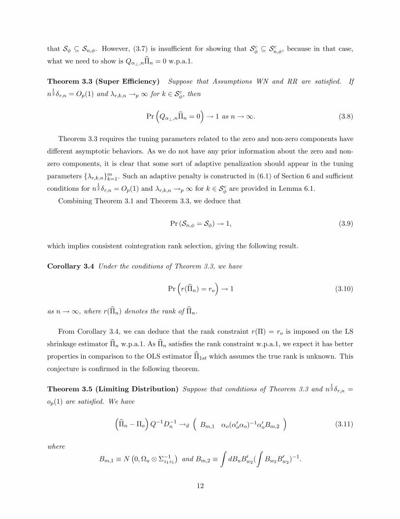
that S� � Sn;�. However, (3.7) is insu¢ cient for showing that Sc� � Scn;�, because in that case,what we need to show is Q�?;nb�n = 0 w.p.a.1.Theorem 3.3 (Super E¢ ciency) Suppose that Assumptions WN and RR are satis�ed. If

n12 �r;n = Op(1) and �r;k;n !p 1 for k 2 Sc�, then

Pr�Q�?;n

b�n = 0�! 1 as n!1: (3.8)

Theorem 3.3 requires the tuning parameters related to the zero and non-zero components have

di¤erent asymptotic behaviors. As we do not have any prior information about the zero and non-

zero components, it is clear that some sort of adaptive penalization should appear in the tuning

parameters f�r;k;ngmk=1. Such an adaptive penalty is constructed in (6.1) of Section 6 and su¢ cientconditions for n

12 �r;n = Op(1) and �r;k;n !p 1 for k 2 Sc� are provided in Lemma 6.1.

Combining Theorem 3.1 and Theorem 3.3, we deduce that

Pr (Sn;� = S�)! 1; (3.9)

which implies consistent cointegration rank selection, giving the following result.

Corollary 3.4 Under the conditions of Theorem 3.3, we have

Pr�r(b�n) = ro�! 1 (3.10)

as n!1, where r(b�n) denotes the rank of b�n.From Corollary 3.4, we can deduce that the rank constraint r(�) = ro is imposed on the LS

shrinkage estimator b�n w.p.a.1. As b�n satis�es the rank constraint w.p.a.1, we expect it has betterproperties in comparison to the OLS estimator b�1st which assumes the true rank is unknown. Thisconjecture is con�rmed in the following theorem.

Theorem 3.5 (Limiting Distribution) Suppose that conditions of Theorem 3.3 and n12 �r;n =

op(1) are satis�ed. We have

�b�n ��o�Q�1D�1n !d

�Bm;1 �o(�

0o�o)

�1�0oBm;2

�(3.11)

where

Bm;1 � N�0;u ��1z1z1

�and Bm;2 �

ZdBuB

0w2(

ZBw2B

0w2)

�1:

12

From (3.11) and the continuous mapping theorem (CMT),

Q�b�n ��o�Q�1D�1n !d

0@ �0oBm;1 �0o�o(�0o�o)

�1�0oBm;2

�0o;?Bm;1 0

1A : (3.12)

Similarly, from Lemma 10.2.(a) in Appendix and CMT

Q�b�1st ��o�Q�1D�1n !d

0@ �0oBm;1 �0oBm;2

�0o;?Bm;1 �0o;?Bm;2

1A : (3.13)

Compared with the OLS estimator, we see that in the LS shrinkage estimation, the right lower

(m � ro) � (m � ro) submatrix of Q�oQ�1 is estimated at a faster rate than n. The improvedproperty of the LS shrinkage estimator b�n arises from the fact that the correct rank restriction

r(b�n) = ro is satis�ed w.p.a.1, leading to the lower right zero block in the limit distribution (3.11)after normalization.

Compared with the oracle reduced rank regression (RRR) estimator (i.e. the RRR estimator in-

formed by knowledge of the true rank, see e.g. Johansen, 1995; Phillips, 1998 and Anderson, 2002),

the LS shrinkage estimator su¤ers from second order bias in the limit distribution (3.11), which is

evident in the endogeneity bias of the factorRdBuB

0w2 in the limit matrix Bm;2. Accordingly, to

remove the endogeneity bias we introduce the generalized least square (GLS) shrinkage estimatorb�g;n which satis�es the weighted extremum problem

b�g;n = argmin�2Rm�m

nXt=1

k�Yt ��Yt�1k2b�1u;n + nmXk=1

�r;k;njj�n;k(�)jj; (3.14)

where bu;n is some consistent estimator of u. GLS methods enable e¢ cient estimation in cointe-grating systems with known rank (Phillips, 1991a, 1991b). Here they are used to achieve e¢ cient

estimation with unknown rank. In fact, the asymptotic distribution of b�g;n is the same as that ofthe oracle RRR estimator.

Corollary 3.6 (Oracle Properties) Suppose Assumptions 3.1 and 3.2 hold. If bu;n !p u and

the tuning parameter satis�es n12 �r;n = op(1) and �r;k;n !p 1 for k 2 Sc�, then

Pr�r(b�g;n) = ro�! 1 as n!1 (3.15)

13

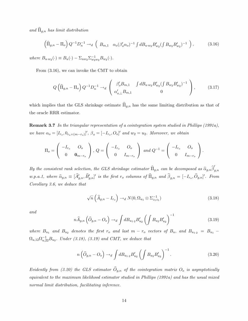
and b�g;n has limit distribution�b�g;n ��o�Q�1D�1n !d

�Bm;1 �o(�

0o�o)

�1 R dBu�w2B0w2(R Bw2B0w2)�1 � ; (3.16)

where Bu�w2(�) � Bu(�)� �uw2��1w2w2Bw2(�).

From (3.16), we can invoke the CMT to obtain

Q�b�g;n ��o�Q�1D�1n !d

0@ �0oBm;1RdBu�w2B

0w2(RBw2B

0w2)

�1

�0o;?Bm;1 0

1A ; (3.17)

which implies that the GLS shrinkage estimate b�g;n has the same limiting distribution as that ofthe oracle RRR estimator.

Remark 3.7 In the triangular representation of a cointegration system studied in Phillips (1991a),

we have �o = [Iro ; 0ro�(m�ro)]0, �o = [�Iro ; Oo]0 and w2 = u2. Moreover, we obtain

�o =

0@ �Iro Oo

0 0m�ro

1A , Q =0@ �Iro Oo

0 Im�ro

1A and Q�1 =

0@ �Iro Oo

0 Im�ro

1A :By the consistent rank selection, the GLS shrinkage estimator b�g;n can be decomposed as b�g;nb�0g;nw.p.a.1, where b�g;n � [ bA0g;n; bB0g;n]0 is the �rst ro columns of b�g;n and b�g;n = [�Iro ; bOg;n]0. FromCorollary 3.6, we deduce that

pn� bAg;n � Iro�!d N(0;u1 ��1z1z1) (3.18)

and

n bAg;n � bOg;n �Oo�!d

ZdBu1�2B

0u2

�ZBu2B

0u2

��1(3.19)

where Bu1 and Bu2 denotes the �rst ro and last m � ro vectors of Bu; and Bu1�2 = Bu1 �u;12

�1u;22Bu2. Under (3.18), (3.19) and CMT, we deduce that

n� bOg;n �Oo�!d

ZdBu1�2B

0u2

�ZBu2B

0u2

��1: (3.20)

Evidently from (3.20) the GLS estimator bOg;n of the cointegration matrix Oo is asymptoticallyequivalent to the maximum likelihood estimator studied in Phillips (1991a) and has the usual mixed

normal limit distribution, facilitating inference.

14

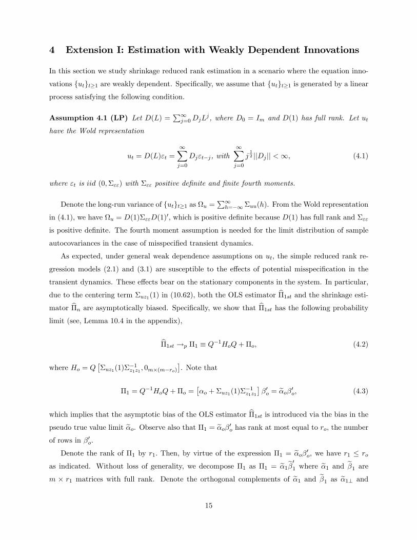
4 Extension I: Estimation with Weakly Dependent Innovations

In this section we study shrinkage reduced rank estimation in a scenario where the equation inno-

vations futgt�1 are weakly dependent. Speci�cally, we assume that futgt�1 is generated by a linearprocess satisfying the following condition.

Assumption 4.1 (LP) Let D(L) =P1j=0DjL

j, where D0 = Im and D(1) has full rank. Let ut

have the Wold representation

ut = D(L)"t =1Xj=0

Dj"t�j, with1Xj=0

j12 jjDj jj <1; (4.1)

where "t is iid (0;�"") with �"" positive de�nite and �nite fourth moments.

Denote the long-run variance of futgt�1 as u =P1h=�1�uu(h). From the Wold representation

in (4.1), we have u = D(1)�""D(1)0, which is positive de�nite because D(1) has full rank and �""

is positive de�nite. The fourth moment assumption is needed for the limit distribution of sample

autocovariances in the case of misspeci�ed transient dynamics.

As expected, under general weak dependence assumptions on ut; the simple reduced rank re-

gression models (2.1) and (3.1) are susceptible to the e¤ects of potential misspeci�cation in the

transient dynamics. These e¤ects bear on the stationary components in the system. In particular,

due to the centering term �uz1(1) in (10.62), both the OLS estimator b�1st and the shrinkage esti-mator b�n are asymptotically biased. Speci�cally, we show that b�1st has the following probabilitylimit (see, Lemma 10.4 in the appendix),

b�1st !p �1 � Q�1HoQ+�o; (4.2)

where Ho = Q��uz1(1)�

�1z1z1 ; 0m�(m�ro)

�. Note that

�1 = Q�1HoQ+�o =

��o +�uz1(1)�

�1z1z1

��0o = e�o�0o; (4.3)

which implies that the asymptotic bias of the OLS estimator b�1st is introduced via the bias in thepseudo true value limit e�o. Observe also that �1 = e�o�0o has rank at most equal to ro; the numberof rows in �0o.

Denote the rank of �1 by r1: Then, by virtue of the expression �1 = e�o�0o, we have r1 � ro

as indicated. Without loss of generality, we decompose �1 as �1 = e�1e�01 where e�1 and e�1 arem � r1 matrices with full rank. Denote the orthogonal complements of e�1 and e�1 as e�1? and

15

e�1? respectively. Similarly, we decompose e�1? as e�1? = (e�?; �o?) where e�? is an m � (ro � r1)matrix. By the de�nition of �1, we know that �o;? is the right eigenvectors of the zero eigenvalues

of �1. Thus, e�1 lies in some subspace of the space spanned by �o. Let Q1 denote the ordered7 lefteigenvector matrix of �1 and de�ne �1;k(�) = Q1(k)�, where Q1(k) denotes the k-th row of Q1.

It is clear that the index set eS� � fk : �1;k(�1) 6= 0g = f1; :::r1g is a subset of S� = fk : �k(�o) 6=0g = f1; :::rog. We next derive the "consistency" of b�n.Corollary 4.1 Let e�r;n = maxk2 eS� �r;k;n, then under Assumptions RR, LP and e�r;n = op(1), theLS shrinkage estimator b�n is consistent, i.e. b�n !p �1.

Corollary 4.1 implies that the shrinkage estimator b�n has the same probability limit as thatof the OLS estimator b�1st. As the pseudo limit �1 may have more zero eigenvalues, comparedwith Theorem 3.1, Corollary 4.1 imposes weaker condition on the tuning parameters f�r;k;ngmk=1.The next corollary provides the convergence rate of the LS shrinkage estimate to the pseudo true

parameter matrix �1.

Corollary 4.2 Under Assumptions RR, LP and e�r;n = op(1), the LS shrinkage estimator b�nsatis�es

(a) if ro = 0, then b�n ��1 = Op(n�1 + n�1e�r;n);(b) if 0 < ro � m, then

�b�n ��1�Q�1D�1n = Op(1 + n12e�r;n).

Recall thatQn is the normalized left eigenvector matrix of b�1st. DecomposeQ0n as hQ0e�;n; Q0e�?;niwhere Qe�;n and Qe�?;n are the �rst r1 and last m� r1 rows of Qn respectively. Under Corollary 4.1and Lemma 10.4.(a),

Qe�;nb�n = Qe�;nb�1st + op(1) = �e�;nQe�;n + op(1) (4.4)

where �e�;n is a diagonal matrix with the ordered �rst (largest) r1 eigenvalues of b�1st. (4.4) andLemma 10.4.(b) implies that the �rst r1 rows of Qnb�n are estimated as nonzero w.p.a.1. On theother hand, by Corollary 4.1 and Lemma 10.4.(a),

Qe�?;nb�n = Qe�?;nb�1st + op(1) = �e�?;nQe�?;n + op(1) (4.5)

where �e�?;n is a diagonal matrix with the ordered last (smallest) m�r1 eigenvalues of b�1st. UnderLemma 10.4.(b) and (c), we know that Qe�?;nb�n converges to zero in probability, while its �rstro � r1 rows and the last m� ro rows have the convergence rates n

12 and n respectively. We next

show that the last m� ro rows of Qnb�n are estimated as zeros w.p.a.1.7The eigenvectors in Q1 are ordered according to the magnitudes of the eigenvalues, i.e. the ordering of the

eigenvalues of �1.

16

Corollary 4.3 (Super E¢ ciency) Under Assumptions LP and RR, if �r;k;n !p 1 for k 2 Sc�and n

12e�r;n = Op(1), then we have

Pr�Qn(k)b�n = 0�! 1 as n!1, (4.6)

for any k 2 Sc�.

Corollary 4.3 implies that b�n has at leastm�ro eigenvalues estimated as zero w.p.a.1. However,the matrix �1 may have more zero eigenvalues than �o. To ensure consistent cointegration rank

selection, we need to show that the ro�r1 zero eigenvalues of �1 are estimated as non-zeros w.p.a.1.From Lemma 10.4, we see that b�1st has m � ro eigenvalues which converge to zero at the rate nand ro � r1 eigenvalues which converge to zero at the rate

pn. The di¤erent convergence rates of

the estimates of the zero eigenvalues of �1 enable us to empirically distinguish the estimates of the

m� ro zero eigenvalues of �1 from the estimates of the ro� r1 zero eigenvalues of �1, as illustratedin the following corollary.

Corollary 4.4 Under Assumptions LP and RR, if n12�r;k;n = op(1) for k 2 fr1 + 1; :::; rog and

n12e�r;n = Op(1), then we have

Pr�Qn(k)b�n 6= 0�! 1 as n!1, (4.7)

for any k 2 fr1 + 1; :::; rog.

In the proof of Corollary 4.4, we show that n12Qn(k)b�n converges in distribution to some non-

degenerated continuous random vectors, which is a stronger result than (4.7). Corollary 4.2 and

Corollary 4.4 implies that b�n has at least m� ro eigenvalues not estimated as zeros w.p.a.1. HenceCorollary 4.2, Corollary 4.3 and Corollary 4.4 give us the following result immediately.

Theorem 4.5 Suppose that Assumptions LP and RR are satis�ed. If n12e�r;n = Op(1), n 1

2�r;k;n =

op(1) for k 2 fr1 + 1; :::; rog and �r;k0;n !p 1 for k0 2 Sc�, then we have

Pr�r(b�n) = ro�! 1 as n!1, (4.8)

as n!1, where r(b�n) denotes the rank of b�n.Compared with Theorem 3.3, Theorem 4.5 imposes similar conditions on the tuning parameters

f�r;k;ngmk=1. It is clear that when the pseudo limit �1 preserves the rank of �o, i.e. ro = r1, we donot need to show Corollary 4.4 because Theorem 4.5 follows by Corollary 4.2 and Corollary 4.3. In

17

that case, Theorem 4.5 imposes the same conditions on the tuning parameters, i.e. n12e�r;n = Op(1)

and �r;k;n !p 1 for k 2 Sc�, where e�r;n = �r;n. On the other hand, when r1 < ro, the conditions inTheorem 4.5 is stronger, because it requires n

12�r;k;n = op(1) for k 2 fr1 + 1; :::; rog. In Section 6,

we construct empirically available tuning parameters which are shown to satisfy the conditions of

Theorem 4.5 without knowing whether r1 = ro or r1 < ro.

Theorem 4.5 states that the true cointegration rank ro can be consistently selected, though

the matrix �o is not consistently estimable. Moreover, when the probability limit �1 of the LS

shrinkage estimator has rank less than ro, Theorem 4.5 ensures that only ro rank is selected in the

LS shrinkage estimation. This result is new in the shrinkage based model selection literature, as the

Lasso-type of techniques are usually advocated because of their ability of shrinking small estimates

(in magnitude) to be zeros in estimation. However, in Corollary 4.4, we show the LS shrinkage

estimation does not shrink the estimates of the extra ro � r1 zero eigenvalues of �1 to be zero.

5 Extension II: Estimation with Explicit Transient Dynamics

This section considers estimation of the general model

�Yt = �oYt�1 +

pXj=1

Bo;j�Yt�j + ut (5.1)

with simultaneous cointegrating rank selection and lag order selection. Recall that the unknown

parameters (�o; Bo) are estimated by penalized LS estimation

(b�n; bBn) = argmin�;B1;:::;Bp2Rm�m

(nXt=1

�Yt ��Yt�1 �Xp

j=1Bj�Yt�j

2+n

pXj=1

�b;j;n kBjk+ nmXk=1

�r;k;n k�n;k(�)k

9=; : (5.2)

For consistent lag order selection the model should be consistently estimable and it is assumed

that the given p in (5.1) is such that the error term ut satis�es Assumption 3.1. De�ne

C(�) = �o +

pXj=0

Bo;j(1� �)�j , where Bo;0 = �Im.

The following assumption extends Assumption 3.2 to accommodate the general structure in (5.1).

Assumption 5.1 (GRR) (i) The determinantal equation jC(�)j = 0 has roots on or outside the

18

unit circle; (ii) the matrix �o has rank ro, with 0 � ro � m; (iii) the (m� ro)� (m� ro) matrix

�0o;?

0@Im � pXj=1

Bo;j

1A�o;? (5.3)

is nonsingular.

Under Assumption 5.1, the time series Yt has the following partial sum representation,

Yt = CB

tXs=1

us + �(L)ut + CBY0 (5.4)

where CB = �o;?h�0o;?

�Im �

Ppj=1Bo;j

��o;?

i�1�0o;? and �(L)ut =

P1s=0 �sut�s is a stationary

process. From the partial sum representation in (5.4), we deduce that �0oYt = �0o�(L)ut and �Yt�j

(j = 0; :::; p) are stationary.

De�ne an m(p+ 1)�m(p+ 1) rotation matrix QB and its inverse Q�1B as

QB �

0BB@�0o 0

0 Imp

�0o;? 0

1CCA and Q�1B =

0@ �o(�0o�o)

�1 0 �o;?(�0o;?�o;?)

�1

0 Imp 0

1A :

Denote �Xt�1 =��Y 0t�1; :::;�Y

0t�p�0 and then the model in (5.1) can be written as

�Yt =h�o Bo

i24 Yt�1

�Xt�1

35+ ut: (5.5)

Let

Zt�1 = QB

24 Yt�1

�Xt�1

35 =24 Z3;t�1Z2;t�1

35 ; (5.6)

where Z 03;t�1 =hY 0t�1�o �X 0

t�1

iis a stationary process and Z2;t�1 = �0o;?Yt�1 comprises the

I(1) components. Denote the index set of the zero components in Bo as ScB such that kBo;jk = 0 forall j 2 ScB and kBo;jk 6= 0 otherwise. We next derive the asymptotic properties of the LS shrinkageestimator (b�n; bBn) de�ned in (5.2).Lemma 5.1 Suppose that Assumptions WN and GRR are satis�ed. If �r;n = op(1) and �b;n = op(1)

where �b;n � maxj2SB �b;j;n, then the LS shrinkage estimator (b�n; bBn) satis�esh(b�n; bBn)� (�o; Bo)iQ�1B D�1n;B = Op(1 + n 1

2 �r;n + n12 �b;n) (5.7)

19

where Dn;B = diag(n�12 Iro+mp; n

�1Im�ro).

Lemma 5.1 implies that the LS shrinkage estimators (b�n; bBn) have the same convergence ratesas the OLS estimators (b�1st; bB1st) (see, Lemma 10.6.a). We next show that if the tuning parameters�r;k;n and �b;j;n (k 2 ScB and j 2 Sc�) converge to zero but not too fast, then the zero rows of Q�oand zero matrices in Bo are estimated as zero w.p.a.1. Let the zero rows of Qnb�n be indexed byScn;� and the zero matrix in bBn be indexed by Scn;B.Theorem 5.1 Suppose that Assumptions WN and GRR are satis�ed. If the tuning parameters

satisfy n12 (�r;n + �b;n) = Op(1), �r;k;n !p 1 and n

12�b;j;n !p 1 for k 2 Sc� and j 2 ScB, then we

have

Pr�Q�;nb�n = 0�! 1 as n!1; (5.8)

and for all j 2 ScBPr� bBn;j = 0m�m�! 1 as n!1: (5.9)

Theorem 5.1 indicates that the zero rows of Q�o (and hence the zero eigenvalues of �o) and

the zero matrices in Bo are estimated as zeros w.p.a.1. Thus Lemma 5.1 and Theorem 5.1 imply

consistent cointegration rank selection and consistent lag order selection.

We next derive the asymptotic distribution of b�S = �b�n; bBSB�, where bBSB denotes the LS

shrinkage estimator of the nonzero matrices in Bo. Let ISB = diag(I1;m; :::; IdSB ;m) where the Ij;m

(j = 1; :::; dSB ) are m � m identity matrices and dSB is the dimensionality of the index set SB:De�ne

QS �

0BB@�0o 0

0 ISB

�0o;? 0

1CCA and Dn;S � diag(n�12 Iro ; n

� 12 ISB ; n

�1Im�ro);

where the identity matrix ISB = ImdSB in QS serves to accommodate the nonzero matrices in Bo.

Let �XS;t denote the nonzero lagged di¤erences in (5.1), then the true model can be written as

�Yt = �oYt�1 +Bo;SB�XS;t�1 + ut = �o;SQ�1S ZS;t�1 + ut (5.10)

where the transformed and reduced regressor variables are

ZS;t�1 = QS

24 Yt�1

�XS;t�1

35 =24 Z3S;t�1Z2;t�1

35 ;

20

with Z 03S;t�1 =hY 0t�1�o �X 0

S;t�1

iand Z2;t�1 = �0o;?Yt�1. From Lemma 10.5, we obtain

n�1nXt=1

Z3S;t�1Z03S;t�1 !p E

�Z3S;t�1Z

03S;t�1

�� �z3Sz3S :

The centred limit theory of b�S is given in the following result.Theorem 5.2 Under conditions of Theorem 5.1, if n

12 (�r;n + �b;n) = op(1), then

�b�S ��o;S�Q�1S D�1n;S !d

�Bm;S �o(�

0o�o)

�1�0oBm;2

�; (5.11)

where

Bm;S � N(0;u ��1z3Sz3S ) and Bm;2 �ZdBuB

0w2(

ZBw2B

0w2)

�1:

Theorem 5.2 extends the result of Theorem 3.5 to the general VECM with lagged di¤erences.

From Theorem 5.2, the LS shrinkage estimator b�S is more e¢ cient than the OLS estimator b�nin the sense that: (i) the zero components in Bo are estimated as zeros w.p.a.1 and thus their LS

shrinkage estimators are super e¢ cient; (ii) under the consistent lagged di¤erences selection, the

true nonzero components in Bo are more e¢ ciently estimated in the sense of smaller asymptotic

variance; and (iii) the true cointegration rank is estimated and therefore when ro < m some parts

of the matrix �o are estimated at a rate faster than root-n.

The LS shrinkage estimator b�n su¤ers from second order asymptotic bias, evident in the com-

ponent Bm;2 of the limit (5.11). As in the simpler model this asymptotic bias is eliminated by GLS

estimation. Accordingly we de�ne the GLS shrinkage estimator of the general model as

(b�g;n; bBg;n) = argmin�;B1;:::;Bp2Rm�m

(nXt=1

�Yt ��Yt�1 �Xp

j=1Bj�Yt�j

2b�1u;n+n

pXj=1

�b;j;n kBjk+ nmXk=1

�r;k;n k�n;k(�)k

9=; : (5.12)

To conclude this section, we show that the GLS shrinkage estimator (b�g;n; bBg;n) is oracle e¢ cientin the sense that it has the same asymptotic distribution as the RRR estimate assuming the true

cointegration rank and lagged di¤erences are known.

Corollary 5.3 (Oracle Properties of GLS) Suppose the conditions of Theorem 5.2 are satis-

�ed. If bu;n !p u, then

Pr�r(b�g;n) = ro�! 1 and Pr

� bBg;j;n = 0�! 1 (5.13)

21

for j 2 ScB as n!1; moreover, b�S has the following limit distribution�b�S ��o;S�Q�1S D�1n;S !d

�Bm;S �o(�

0o�o)

�1 R dBu�w2B0w2(R Bw2B0w2)�1 � (5.14)

where Bu�w2 is de�ned in Theorem 3.6.

Corollary 5.3 is proved using the same arguments as Corollary 3.6 and Theorem 5.2. Its proof

is omitted. The asymptotic distributions of the penalized LS/GLS estimates can be used to con-

duct inference on �o and Bo. However, use of these asymptotic distributions implies that the true

cointegrating rank and lag order are selected with probability one. In consequence, these distribu-

tions may provide poor approximations to the �nite sample distributions of the penalized LS/GLS

estimates when model selection errors occur in �nite samples, leading to potential size distortions

in inference based on (5.11) or (5.14). The development of robust approaches to con�dence interval

construction therefore seems an important task for future research.

Remark 5.4 Although the grouped Lasso penalty function P (B) = kBk is used in LS shrinkageestimation (5.2) and GLS shrinkage estimation (5.12), we remark that a full Lasso penalty function

can also be used and the resulting GLS shrinkage estimate enjoys the same properties stated in

Corollary 5.3. The GLS shrinkage estimation using the (full) Lasso penalty takes the following

form

(b�g;n; bBg;n) = argmin�;B1;:::;Bp2Rm�m

(nXt=1

�Yt ��Yt�1 �Xp

j=1Bj�Yt�j

2b�1u;n+n

pXj=1

mXl=1

mXs=1

�b;j;l;s;njBj;lsj+ nmXk=1

�r;k;n k�n;k(�)k

9=;(5.15)

where Bj;ls denotes the (l; s)-th element of Bj. The advantage of the grouped Lasso penalty P (B)

is that it shrinks elements in B to zero groupwisely, which makes it a natural choice for the lag

order selection (as well as lag elimination) in VECMs. The Lasso penalty is more �exible and when

used in shrinkage estimation, it can do more than select the zero matrices. It can also select the

non-zero elements in the nonzero matrices Bo;j (j 2 SB) w.p.a.1.

Remark 5.5 The �exibility of the Lasso penalty enables GLS shrinkage estimation to achieve more

goals in one-step, in addition to model selection and e¢ cient estimation. Suppose that the vector Yt

can be divided in r and m�r dimensional subvectors Y1;t and Y2;t, then the VECM can be rewritten

22

as 24 �Y1;t�Y2;t

35 =

24 �11o �12o

�21o �22o

3524 Y1;t�1Y2;t�1

35+ pXj=1

24 B11o;j B12o;j

B21o;j B22o;j

3524 �Y1;t�j�Y2;t�j

35+ ut;(5.16)

where �o and Bo;j (j = 1; ::; p) are partitioned in line with Yt. By de�nition, Y2;t does not Granger-

cause Y1;t if and only if

�12o = 0 and B12o;j = 0 for any j 2 SB.

One can attach the (grouped) Lasso penalty of �12 in (5.16) such that the causality test is auto-

matically executed in GLS shrinkage estimation.

Remark 5.6 In this paper, we only consider the Lasso penalty function in the LS or GLS shrink-

age estimation. The main advantage of the Lasso penalty is that it is a convex function, which

combines the convexity of the LS or GLS criterion, making the computation of the shrinkage esti-

mate faster and more accurate. It is clear that as long as the tuning parameter satis�es certain rate

requirements, our main results continue to hold if other penalty functions (e.g., the bridge penalty)

are used in the LS or GLS shrinkage estimation.

6 Adaptive Selection of the Tuning Parameters

This section develops a data-driven procedure of selecting the tuning parameters f�r;k;ngmk=1 andf�b;j;ngpj=1. As presented in previous sections, the conditions ensuring oracle properties in GLSshrinkage estimation require that the tuning parameters of the estimates of zero and nonzero

components have di¤erent asymptotic behavior. For example, in Theorem 3.3, we need �r;k;n =

Op(n� 12 ) for any k 2 S� and �r;k;n !p 1 for k 2 Sc�, which implies that some sort of known

adaptive penalty should appear in �r;k;n. One popular choice of such a penalty is the adaptive

Lasso penalty (c.f., Zou, 2006), which in our model can be de�ned as

�r;k;n =��r;k;n

jj�k(b�1st)jj! and �b;j;n =m!��b;j;n

jj bB1st;j jj! (6.1)

where ��r;k;n and ��b;j;n are non-increasing positive sequences and ! is some positive �nite constant.

The adaptive penalty in �r;k;n is jj�k(b�1st)jj�! (k = 1; :::;m), because for any k 2 Sc�, thereis jj�k(b�1st)jj�! !p 1 and for any k 2 S�, there is jj�k(b�1st)jj�! !p jj�k(�o)jj�! = O(1) under

23

Assumption WN8. Similarly, the adaptive penalty in �b;j;n is m!jj bB1st;j jj�!, where the extra termm! is used to adjust the e¤ect of dimensionality of Bj on the adaptive penalty. Such adjustment

does not e¤ect the asymptotic properties of the LS/GLS shrinkage estimation, but it is used to

improve their �nite sample performances. To see the e¤ect of the dimensionality on the adaptive

penalty, we write

jj bB1st;j jj! = " mXl=1

mXh=1

��� bB1st;j;lh���2#!2

:

Although each individual j bB1st;j;lhj2 may be close to zero, jj bB1st;j jj2 could be large in magnitude in�nite samples because it is the sum of m2 such terms (i.e. j bB1st;j;lhj2). As a result, the adaptivepenalty jj bB1st;j jj�! without any adjustment tends to be smaller than the value it should be. Onestraightforward adjustment for the dimensionality e¤ect is to use the average, instead of the sum,

of the square terms j bB1st;j;lhj2, i.e."m�2

mXl=1

mXh=1

j bB1st;j;lhj2#!2

= m�!jj bB1st;j jj!in the adaptive penalty. Under some general rate conditions on ��r;k;n and �

�b;j;n, the following

lemma shows that the tuning parameters speci�ed in (6.1) satisfy the conditions in our theorems

of super e¢ ciency and oracle properties.

Lemma 6.1 (i) If n12��r;k;n = o(1) and n!��r;k;n ! 1, then under Assumptions WN and RR we

have

n12 �r;n = op(1) and �r;k;n !p 1

for any k 2 Sc�; (ii) if n1+!2 ��r;k;n = o(1) and n

!��r;k;n !1, then under Assumptions LP and RR

n12e�r;n = op(1), n 1

2�r;k;n = op(1) and �r;k0;n !p 1

for any k 2 fr1 + 1; :::; rog and k0 2 Sc�; (iii) if n12��r;k;n = o(1) and n!��r;k;n ! 1 for any

k = 1; :::;m, and n12��b;j;n = o(1) and n

1+!2 ��b;j;n !1 for any j = 1; :::; p, then under Assumptions

WN and GRR

n12 (�r;n + �b;n) = op(1), �r;k;n !p 1 and �b;j;n !p 1

for any k 2 Sc� and j 2 ScB.

It is notable that, when ut is iid, ��r;k;n is required to converge to zero with the rate faster than

8The same intuition applies to the scenario where Assumption LP holds.

24

n�12 , while when ut is weakly dependent, ��r;k;n has to converge to zero with the rate faster than

n�1+!2 . The convergence rate of ��r;k;n in Lemma 6.1.(ii) is faster to ensure that the pseudo ro � r1

zero eigenvalues in �1 are estimated as non-zeros w.p.a.1. When r1 = ro, �1 contains no pseudo zero

eigenvalues and it has the true rank ro. It is clear that in this case, we only need n12��r;k;n = o(1) and

n!��r;k;n !1 to show that the tuning parameters in (6.1) satisfy n12 �r;n = op(1) and �r;k0;n !p 1

for any k0 2 Sc�.From Lemma 6.1, we see that the conditions imposed on

���r;k;n

mk=1

and f��b;j;ngpj=1 to ensure

oracle properties in GLS shrinkage estimation only restrict the rates at which the sequences ��r;k;n

and ��b;j;n go to zero. But in �nite samples these conditions are not precise enough to provide

a clear choice of tuning parameter for practical implementation. On one hand these sequences

should converge to zero as fast as possible so that shrinkage bias in the estimation of the nonzero

components of the model is as small as possible. In the extreme case where ��r;k;n = 0 and ��b;j;n = 0,

LS shrinkage estimation reduces to LS estimation and there is no shrinkage bias in the resulting

estimators. (Of course there may still be �nite sample estimation bias). On the other hand, these

sequences should converge to zero as slow as possible so that in �nite samples zero components in

the model are estimated as zeros with higher probability. In the opposite extremity ��r;k;n = 1and ��b;j;n = 1, and then all parameters of the model are estimated as zeros with probability onein �nite samples. Thus there is bias and variance trade-o¤ in the selection of the sequences in���r;k;n

mk=1

and f��b;j;ngpj=1.

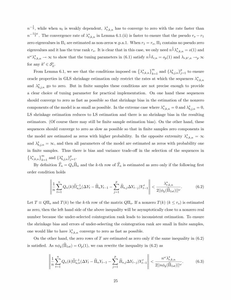
By de�nition bTn = Qnb�n and the k-th row of bTn is estimated as zero only if the following �rstorder condition holds 1n

nXt=1

Qn(k)b�1u;n(�Yt � b�nYt�1 � pXj=1

bBn;j�Yt�j)Y 0t�1 < ��r;k;n

2jj�k(b�1st)jj! : (6.2)

Let T � Q�o and T (k) be the k-th row of the matrix Q�o. If a nonzero T (k) (k � ro) is estimatedas zero, then the left hand side of the above inequality will be asymptotically close to a nonzero real

number because the under-selected cointegration rank leads to inconsistent estimation. To ensure

the shrinkage bias and errors of under-selecting the cointegration rank are small in �nite samples,

one would like to have ��r;k;n converge to zero as fast as possible.

On the other hand, the zero rows of T are estimated as zero only if the same inequality in (6.2)

is satis�ed. As n�k(b�1st) = Op(1), we can rewrite the inequality in (6.2) as 1nnXt=1

Qn(k)b�1u;n(�Yt � b�nYt�1 � pXj=1

bBn;j�Yt�j)Y 0t�1 < n!��r;k;n

2jjn�k(b�1st)jj! : (6.3)

25

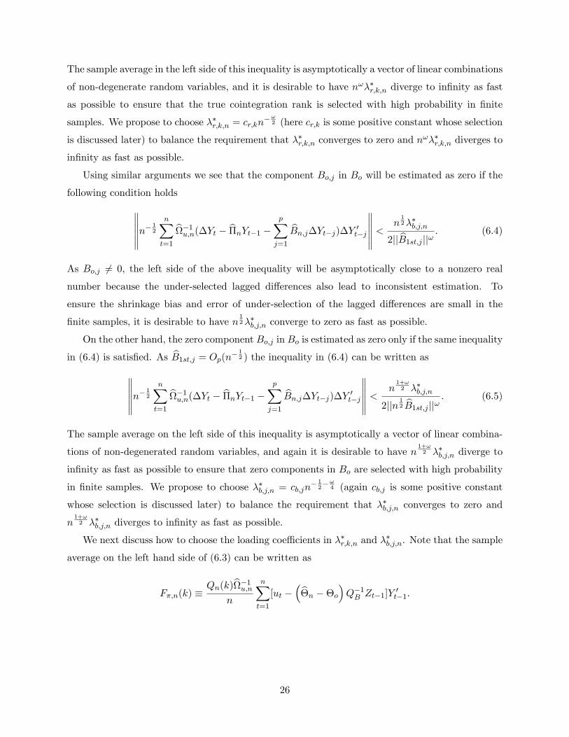
The sample average in the left side of this inequality is asymptotically a vector of linear combinations

of non-degenerate random variables, and it is desirable to have n!��r;k;n diverge to in�nity as fast

as possible to ensure that the true cointegration rank is selected with high probability in �nite

samples. We propose to choose ��r;k;n = cr;kn�!2 (here cr;k is some positive constant whose selection

is discussed later) to balance the requirement that ��r;k;n converges to zero and n!��r;k;n diverges to

in�nity as fast as possible.

Using similar arguments we see that the component Bo;j in Bo will be estimated as zero if the

following condition holds n� 12

nXt=1

b�1u;n(�Yt � b�nYt�1 � pXj=1

bBn;j�Yt�j)�Y 0t�j < n

12��b;j;n

2jj bB1st;j jj! : (6.4)

As Bo;j 6= 0, the left side of the above inequality will be asymptotically close to a nonzero real

number because the under-selected lagged di¤erences also lead to inconsistent estimation. To

ensure the shrinkage bias and error of under-selection of the lagged di¤erences are small in the

�nite samples, it is desirable to have n12��b;j;n converge to zero as fast as possible.

On the other hand, the zero component Bo;j in Bo is estimated as zero only if the same inequality

in (6.4) is satis�ed. As bB1st;j = Op(n� 12 ) the inequality in (6.4) can be written as n� 1

2

nXt=1

b�1u;n(�Yt � b�nYt�1 � pXj=1

bBn;j�Yt�j)�Y 0t�j < n

1+!2 ��b;j;n

2jjn 12 bB1st;j jj! : (6.5)

The sample average on the left side of this inequality is asymptotically a vector of linear combina-

tions of non-degenerated random variables, and again it is desirable to have n1+!2 ��b;j;n diverge to

in�nity as fast as possible to ensure that zero components in Bo are selected with high probability

in �nite samples. We propose to choose ��b;j;n = cb;jn� 12�!4 (again cb;j is some positive constant

whose selection is discussed later) to balance the requirement that ��b;j;n converges to zero and

n1+!2 ��b;j;n diverges to in�nity as fast as possible.

We next discuss how to choose the loading coe¢ cients in ��r;k;n and ��b;j;n. Note that the sample

average on the left hand side of (6.3) can be written as

F�;n(k) �Qn(k)b�1u;n

n

nXt=1

[ut ��b�n ��o�Q�1B Zt�1]Y 0t�1:

26

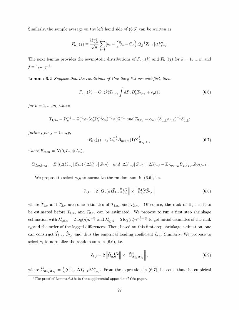
Similarly, the sample average on the left hand side of (6.5) can be written as

Fb;n(j) �b�1u;npn

nXt=1

[ut ��b�n ��o�Q�1B Zt�1]�Y 0t�j :

The next lemma provides the asymptotic distributions of F�;n(k) and Fb;n(j) for k = 1; :::;m and

j = 1; :::; p.9

Lemma 6.2 Suppose that the conditions of Corollary 5.3 are satis�ed, then

F�;n(k) = Qn(k)T1;�o

ZdBuB

0uT2;�o + op(1) (6.6)

for k = 1; :::;m, where

T1;�o = �1u � �1u �o(�0o�1u �o)�1�0o�1u and T2;�o = �o;?(�

0o;?�o;?)

�1�0o;?;

further, for j = 1; :::; p,

Fb;n(j)!d � 12

u Bm�m(1)�12

�yj jz3S (6.7)

where Bm;m = N(0; Im Im),

��yj jz3S = E�(�Yt�j jZ3S)

��Y 0t�j

��Z3S�� and �Yt�j jZ3S = �Yt�j � ��yjz3S��1z3Sz3SZ3S;t�1:

We propose to select cr;k to normalize the random sum in (6.6), i.e.

bcr;k = 2 Qn(k) bT1;�b1=2u;n � b1=2u;n bT2;� (6.8)

where bT1;� and bT2;� are some estimates of T1;�o and T2;�o . Of course, the rank of �o needs tobe estimated before T1;�o and T2;�o can be estimated. We propose to run a �rst step shrinkage

estimation with ��r;k;n = 2 log(n)n�!2 and ��b;j;n = 2 log(n)n

� 12�!4 to get initial estimates of the rank

ro and the order of the lagged di¤erences. Then, based on this �rst-step shrinkage estimation, one

can construct bT1;�, bT2;� and thus the empirical loading coe¢ cient bcr;k. Similarly, We propose toselect cb to normalize the random sum in (6.6), i.e.

bcb;j = 2 b�1=2u;n

� b� 12�yj�yj

; (6.9)

where b��yj�yj = 1n

Pnt=1�Yt�j�Y

0t�j . From the expression in (6.7), it seems that the empirical

9The proof of Lemma 6.2 is in the supplemental appendix of this paper.

27

analog of ��yj jz3S is a more propriate term to normalize Fb;n(j). However, if �Yt�j is a redundant

lag and the residual of its projection on �0oYt�1 and non-redundant lagged di¤erences is close to

zero, then ��yj jz3S and its estimate will be close to zero. As a result, bcb;j tends to be small,which will increase the probability of including �Yt�j in the selected model with higher probability

in �nite samples. To avoid such unappealing scenario, we use b��yj�yj instead of the empiricalanalog of ��yj jz3S in (6.9). It is clear that bcb;j can be directly constructed from the preliminary LS

estimation.

The choice of ! is a more complicated issue which is not pursued in this paper. For the empirical

applications, we propose to choose ! = 2 because such a choice is popular in the Lasso-based

variable selection literature, it satis�es all our rate criteria, and simulations show that the choice

works remarkably well. Based on all the above results, we propose the following data dependent

tuning parameters for LS shrinkage estimation:

�r;k;n =2

n

Qn(k) bT1;�b1=2u;n � b1=2u;n bT2;� � jj�k(b�1st)jj�2 (6.10)

and

�b;j;n =2m2

n

b�1=2u;n

� b� 12�yj�yj

� jj bB1st;j jj�2 (6.11)

for k = 1; :::;m and j = 1; :::; p. The above discussion is based on the general VECM with iid ut.

In the simple error correction model where the cointegration rank selection is the only concern,

the adaptive tuning parameters proposed in (6.10) are still valid. The expression in (6.10) will be

invalid when ut is weakly dependent and r1 < ro. In that case, we propose to replace the leading

term 2n�1 in (6.10) by 2n�3=2.

7 Simulation Study

We conducted simulations to assess the �nite sample performance of the shrinkage estimates in

terms of cointegrating rank selection and e¢ cient estimation. Three models were investigated. In

the �rst model, the simulated data are generated from0@ �Y1;t

�Y2;t

1A = �o

0@ Y1;t�1

Y2;t�1

1A+0@ u1;t

u2;t

1A ; (7.1)

28

where ut � iid N(0;u) with u =

0@ 1 0:5

0:5 0:75

1A. The initial observation Y0 is set to be zero forsimplicity. �o is speci�ed as follows0@ �11;o �12;o

�21;o �22;o

1A =

0@ 0 0

0 0

1A ,0@ �1 �0:5

1 0:5

1A and

0@ �0:5 0:1

0:2 �0:4

1A (7.2)

to allow for the cointegration rank to be 0, 1 and 2 respectively.

In the second model, the simulated data fYtgnt=1 are generated from equations (7.1)-(7.2), whilethe innovation term ut is generated by0@ u1;t

u2;t

1A =

0@ 1 0:5

0:5 0:75

1A0@ u1;t�1

u2;t�1

1A+0@ "1;t

"2;t

1A ,where "t � iid N(0;") with " = diag(1:25; 0:75). The initial values Y0 and "0 are set to be zero.

The third model has the following form0@ �Y1;t

�Y2;t

1A = �o

0@ Y1;t�1

Y2;t�1

1A+B1;o0@ �Y1;t�1

�Y2;t�1

1A+B3;o0@ �Y1;t�3

�Y2;t�3

1A+ ut; (7.3)

where ut is generated under the same condition in (7.1), �o is speci�ed similarly in (7.2), B1;o and

B3;o are taken to be diag(0:4; 0:4) such that Assumption 5.1 is satis�ed. The initial values (Yt; "t)

(t = �3; :::; 0) are set to be zero. In the above three cases, we include 50 additional observationsto the simulated sample with sample size n to eliminate start-up e¤ects from the initialization.

In the �rst two models, we assume that the econometrician speci�es the following model0@ �Y1;t

�Y2;t

1A = �o

0@ Y1;t�1

Y2;t�1

1A+ ut; (7.4)

where ut is iid(0;u) with some unknown positive de�nite matrix u. The above empirical model is

correctly speci�ed under the data generating assumption (7.1), but is misspeci�ed under (7.2). We

are interested in investigating the performance of the shrinkage method in selecting the correct rank

of �o under both data generating assumptions and e¢ cient estimation of �o under Assumption

(7.1).

29

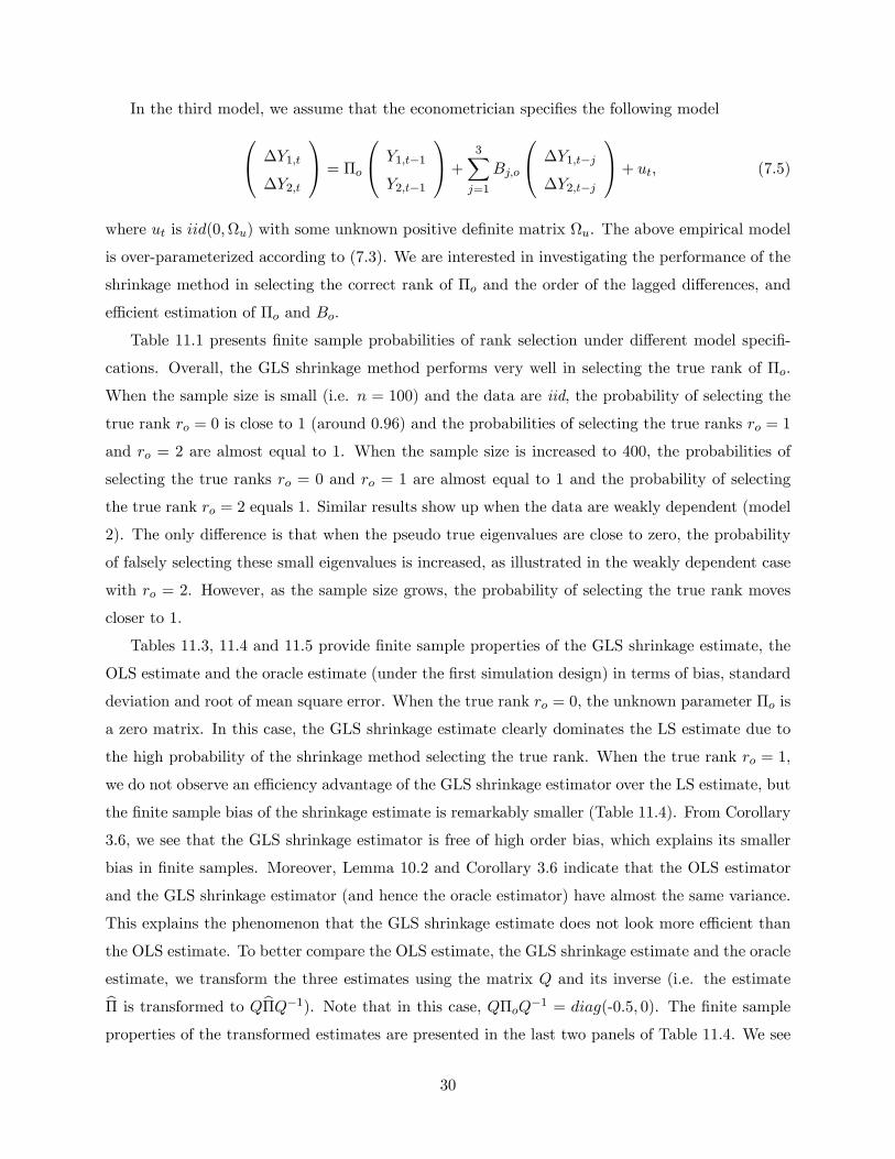
In the third model, we assume that the econometrician speci�es the following model0@ �Y1;t

�Y2;t

1A = �o

0@ Y1;t�1

Y2;t�1

1A+ 3Xj=1

Bj;o

0@ �Y1;t�j

�Y2;t�j

1A+ ut; (7.5)

where ut is iid(0;u) with some unknown positive de�nite matrix u. The above empirical model

is over-parameterized according to (7.3). We are interested in investigating the performance of the

shrinkage method in selecting the correct rank of �o and the order of the lagged di¤erences, and

e¢ cient estimation of �o and Bo.

Table 11.1 presents �nite sample probabilities of rank selection under di¤erent model speci�-

cations. Overall, the GLS shrinkage method performs very well in selecting the true rank of �o.

When the sample size is small (i.e. n = 100) and the data are iid, the probability of selecting the

true rank ro = 0 is close to 1 (around 0.96) and the probabilities of selecting the true ranks ro = 1

and ro = 2 are almost equal to 1. When the sample size is increased to 400, the probabilities of

selecting the true ranks ro = 0 and ro = 1 are almost equal to 1 and the probability of selecting

the true rank ro = 2 equals 1. Similar results show up when the data are weakly dependent (model

2). The only di¤erence is that when the pseudo true eigenvalues are close to zero, the probability

of falsely selecting these small eigenvalues is increased, as illustrated in the weakly dependent case

with ro = 2. However, as the sample size grows, the probability of selecting the true rank moves

closer to 1.

Tables 11.3, 11.4 and 11.5 provide �nite sample properties of the GLS shrinkage estimate, the

OLS estimate and the oracle estimate (under the �rst simulation design) in terms of bias, standard

deviation and root of mean square error. When the true rank ro = 0, the unknown parameter �o is

a zero matrix. In this case, the GLS shrinkage estimate clearly dominates the LS estimate due to

the high probability of the shrinkage method selecting the true rank. When the true rank ro = 1,

we do not observe an e¢ ciency advantage of the GLS shrinkage estimator over the LS estimate, but

the �nite sample bias of the shrinkage estimate is remarkably smaller (Table 11.4). From Corollary

3.6, we see that the GLS shrinkage estimator is free of high order bias, which explains its smaller

bias in �nite samples. Moreover, Lemma 10.2 and Corollary 3.6 indicate that the OLS estimator

and the GLS shrinkage estimator (and hence the oracle estimator) have almost the same variance.

This explains the phenomenon that the GLS shrinkage estimate does not look more e¢ cient than

the OLS estimate. To better compare the OLS estimate, the GLS shrinkage estimate and the oracle

estimate, we transform the three estimates using the matrix Q and its inverse (i.e. the estimateb� is transformed to Qb�Q�1). Note that in this case, Q�oQ�1 = diag(-0:5; 0). The �nite sampleproperties of the transformed estimates are presented in the last two panels of Table 11.4. We see

30

that the elements in the last column of the transformed GLS shrinkage estimator enjoys very small

bias and small variance even when the sample size is only 100. The elements in the last column

of the OLS estimator, when compared with the elements in its �rst column, have smaller variance

but larger bias. It is clear that as the sample size grows, the GLS shrinkage estimator approaches

the oracle estimator in terms of overall performance. When the true rank ro = 2, the LS estimator

is better than the shrinkage estimator as the latter su¤ers from shrinkage bias in �nite samples. If

shrinkage bias is a concern, one can run a reduced rank regression based on the rank selected by the

GLS shrinkage estimation to get the so called post-Lasso estimator (c.f. Belloni and Chernozhukov,

2013). The post-Lasso estimator also enjoys oracle properties and it is free of shrinkage bias in

�nite samples.

Table 11.2 shows �nite sample probabilities of the new shrinkage method in joint rank and lag

order selection for the third model. Evidently, the method performs very well in selecting the true

rank and true lagged di¤erences (and thus the true model) in all scenarios.10 It is interesting to see

that the probabilities of selecting the true ranks are not negatively a¤ected either by adding lags

to the model or by the lagged order selection being simultaneously performed with rank selection.

Tables 11.6, 11.7 and 11.8 present the �nite sample properties of GLS shrinkage, OLS, and oracle

estimation. When compared with the oracle estimates, some components in the GLS shrinkage

estimate even have smaller variances, though their �nite sample biases are slightly larger. As a

result, their root mean square errors are smaller than these of their counterparts in oracle estimation.

Moreover, the GLS shrinkage estimate generally has smaller variance when compared with the OLS

estimate, though the �nite sample bias of the shrinkage estimate of nonzero component is slightly

larger, as expected. The intuition that explains how the GLS shrinkage estimate can outperform

the oracle estimate lies in the fact that there are some zero components in Bo and shrinking their

estimates towards zero (but not exactly to zero) helps to reduce their bias and variance. From

this perspective, the shrinkage estimates of the zero components in Bo share features similar to

traditional shrinkage estimates, revealing that �nite sample shrinkage bias is not always harmful.

Additional simulations were conducted to compare the performance of our least squares (LS)

shrinkage techniques with the direct use of information criteria for model determination. The results

are summarized here and presented in full in the Supplemental Appendix (Liao and Phillips, 2013).

Amongst the usual information criteria, we �nd that BIC outperforms AIC and HQ and does well

in selecting cointegrating rank even when the sample size is as small as n = 100; corroborating

10Joint determination of the lagged di¤erences and cointegration rank can also be performed using informationcriteria like AIC and BIC, as suggested in Phillips and McFarland (1997) and Chao and Phillips (1999). As discussedbelow, the supplemental appendix provides simulation comparisons between information criteria and LS shrinkageestimation.

31

earlier �ndings in Cheng and Phillips (2009, 2012). In the determination of transient dynamic

structure, information criteria typically proceed by way of sequential selection working from the

most general model to the most restrictive, largely for convenience and computational simplicity.

Accordingly, these methods commonly miss true transient dynamic structures in which some subsets

of lag coe¢ cients are zero. In such cases, BIC and the other criteria may select the maximum lag

correctly but miss the more complex dynamic structure. In comparison, LS shrinkage estimation

performs well in selecting the true transient dynamic structure, the maximum lag in the transient

dynamics, and the cointegrating rank.

8 An Empirical Example

This section reports an empirical example to illustrate the application of these techniques to time

series modeling of long-run and short-run behavior of aggregate income, consumption and invest-

ment in the US economy. The sample11 used in the empirical study is quarterly data over the

period 1947-2009 from the Federal Reserve Economic Data (FRED).

1947:1 1953:2 1959:3 1965:4 1972:1 1978:2 1984:3 1990:4 1997:1 2003:2 2009:30

10

20

30

40

50

Real ConsumptionReal IncomeReal Investment

Figure 8.1. US GNP, Consumption and Investment in logarithms and in 2005

dollars. Data Source: Federal Reserve Economic Data (FRED) St. Louis Fed

The sample data are shown in Figure 8.1. Evidently, the time series display long-term trend

growth, which is especially clear in GNP and consumption, and some commonality in the growth

mechanism over time. In particular, the series show evidence of some co-movement over the entire

11We thank George Athanasopoulos for providing the data.

32

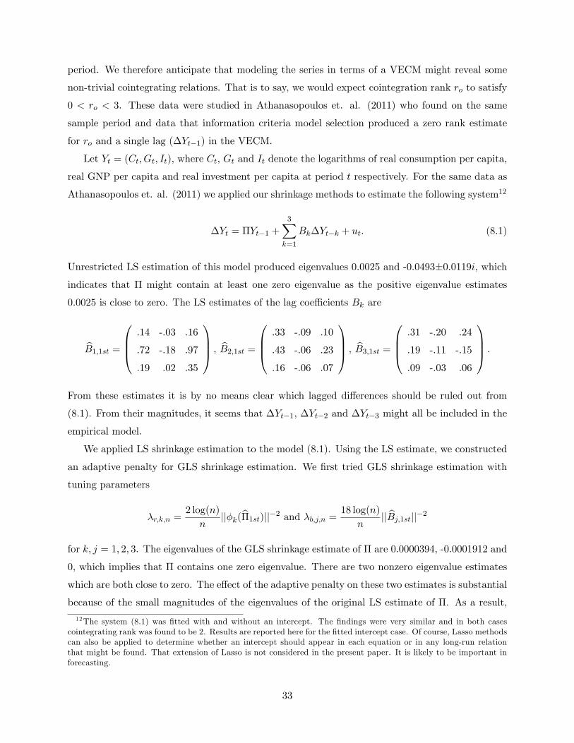
period. We therefore anticipate that modeling the series in terms of a VECM might reveal some

non-trivial cointegrating relations. That is to say, we would expect cointegration rank ro to satisfy

0 < ro < 3. These data were studied in Athanasopoulos et. al. (2011) who found on the same

sample period and data that information criteria model selection produced a zero rank estimate

for ro and a single lag (�Yt�1) in the VECM.

Let Yt = (Ct; Gt; It), where Ct, Gt and It denote the logarithms of real consumption per capita,

real GNP per capita and real investment per capita at period t respectively. For the same data as

Athanasopoulos et. al. (2011) we applied our shrinkage methods to estimate the following system12

�Yt = �Yt�1 +3Xk=1

Bk�Yt�k + ut. (8.1)

Unrestricted LS estimation of this model produced eigenvalues 0.0025 and -0.0493�0.0119i, whichindicates that � might contain at least one zero eigenvalue as the positive eigenvalue estimates

0.0025 is close to zero. The LS estimates of the lag coe¢ cients Bk are

bB1;1st =0BB@.14 -.03 .16

.72 -.18 .97

.19 .02 .35

1CCA , bB2;1st =0BB@.33 -.09 .10

.43 -.06 .23

.16 -.06 .07

1CCA , bB3;1st =0BB@.31 -.20 .24

.19 -.11 -.15

.09 -.03 .06

1CCA :From these estimates it is by no means clear which lagged di¤erences should be ruled out from

(8.1). From their magnitudes, it seems that �Yt�1, �Yt�2 and �Yt�3 might all be included in the

empirical model.

We applied LS shrinkage estimation to the model (8.1). Using the LS estimate, we constructed

an adaptive penalty for GLS shrinkage estimation. We �rst tried GLS shrinkage estimation with

tuning parameters

�r;k;n =2 log(n)

njj�k(b�1st)jj�2 and �b;j;n = 18 log(n)

njj bBj;1stjj�2

for k; j = 1; 2; 3. The eigenvalues of the GLS shrinkage estimate of � are 0.0000394, -0.0001912 and

0, which implies that � contains one zero eigenvalue. There are two nonzero eigenvalue estimates

which are both close to zero. The e¤ect of the adaptive penalty on these two estimates is substantial

because of the small magnitudes of the eigenvalues of the original LS estimate of �. As a result,

12The system (8.1) was �tted with and without an intercept. The �ndings were very similar and in both casescointegrating rank was found to be 2. Results are reported here for the �tted intercept case. Of course, Lasso methodscan also be applied to determine whether an intercept should appear in each equation or in any long-run relationthat might be found. That extension of Lasso is not considered in the present paper. It is likely to be important inforecasting.

33

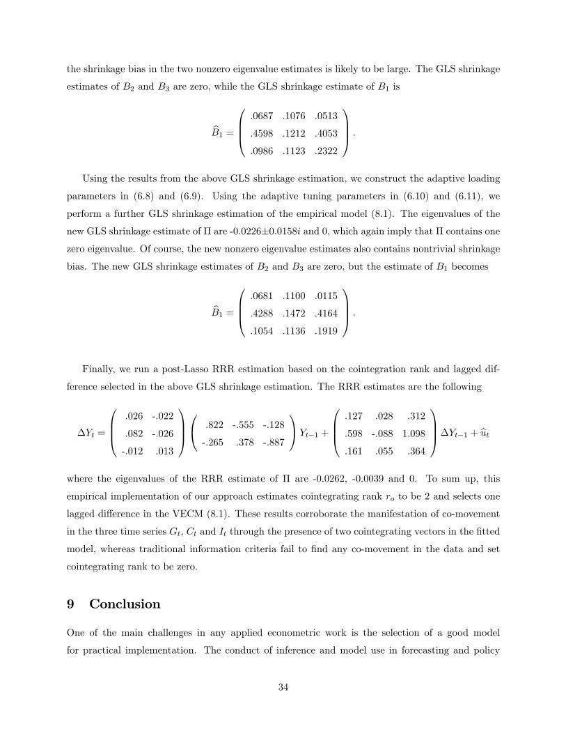
the shrinkage bias in the two nonzero eigenvalue estimates is likely to be large. The GLS shrinkage

estimates of B2 and B3 are zero, while the GLS shrinkage estimate of B1 is

bB1 =0BB@.0687 .1076 .0513

.4598 .1212 .4053

.0986 .1123 .2322

1CCA .Using the results from the above GLS shrinkage estimation, we construct the adaptive loading

parameters in (6.8) and (6.9). Using the adaptive tuning parameters in (6.10) and (6.11), we

perform a further GLS shrinkage estimation of the empirical model (8.1). The eigenvalues of the

new GLS shrinkage estimate of � are -0.0226�0.0158i and 0, which again imply that � contains onezero eigenvalue. Of course, the new nonzero eigenvalue estimates also contains nontrivial shrinkage

bias. The new GLS shrinkage estimates of B2 and B3 are zero, but the estimate of B1 becomes

bB1 =0BB@.0681 .1100 .0115

.4288 .1472 .4164

.1054 .1136 .1919

1CCA .

Finally, we run a post-Lasso RRR estimation based on the cointegration rank and lagged dif-

ference selected in the above GLS shrinkage estimation. The RRR estimates are the following

�Yt =

0BB@.026 -.022

.082 -.026

-.012 .013

1CCA0@ .822 -.555 -.128

-.265 .378 -.887

1AYt�1 +0BB@.127 .028 .312

.598 -.088 1.098

.161 .055 .364

1CCA�Yt�1 + butwhere the eigenvalues of the RRR estimate of � are -0.0262, -0.0039 and 0. To sum up, this

empirical implementation of our approach estimates cointegrating rank ro to be 2 and selects one

lagged di¤erence in the VECM (8.1). These results corroborate the manifestation of co-movement

in the three time series Gt, Ct and It through the presence of two cointegrating vectors in the �tted

model, whereas traditional information criteria fail to �nd any co-movement in the data and set

cointegrating rank to be zero.

9 Conclusion

One of the main challenges in any applied econometric work is the selection of a good model

for practical implementation. The conduct of inference and model use in forecasting and policy

34

analysis are inevitably conditioned on the empirical process of model selection, which typically leads

to issues of post-model selection inference. Adaptive Lasso and bridge estimation methods provide

a methodology where these di¢ culties may be partly attenuated by simultaneous model selection

and estimation to facilitate empirical research in complex models like reduced rank regressions

where many selection decisions need to be made to construct a satisfactory empirical model. On

the other hand, as indicated in the Introduction, the methods certainly do not eliminate post-

shrinkage selection inference issues in �nite samples because the estimators carry the e¤ects of the

in-built selections.

This paper shows how to use the methodology of shrinkage in a multivariate system to develop an

automated approach to cointegrated system modeling that enables simultaneous estimation of the

cointegrating rank and autoregressive order in conjunction with oracle-like e¢ cient estimation of the

cointegrating matrix and the transient dynamics. As such the methods o¤er practical advantages to

the empirical researcher by avoiding sequential techniques where cointegrating rank and transient

dynamics are estimated prior to model �tting.

As indicated in the Introduction, sequential methods can encounter obstacles to consistent order

estimation even when test size is driven to zero as the sample size n ! 1: For instance, in themodel (7.3) considered earlier

�Yt = �oYt�1 +Bo;1�Yt�1 +Bo;2�Yt�2 +Bo;3�Yt�3 + ut;

where kBo;2k = 0, kBo;1k 6= 0 and kBo;3k 6= 0. It is clear that in this model both upward and

downward sequential testing procedures either include the second lag di¤erence or exclude it to-

gether with the third lag di¤erence. As a result, the true model is never correctly selected by such

standard algorithms - much more intensive searches are required. In the more general model

�Yt = �oYt�1 +

pXj=1

Bo;j�Yt�j + ut

where p is large but �xed, the model selection limitations of standard sequential testing are in-

evitably worse, although these may be mitigated by orthonormalization, parsimonious encompass-

ing, and other automated devices (Hendry and Krolzig, 2005; Hendry and Johansen, 2013). The

methods of the present paper do not require any speci�c order or format of the lag di¤erences to

ensure consistent model selection. As a result, the approach is invariant to permutations of the

order of the lag di¤erences. Moreover, the method is easier to implement in empirical work, requires

no intensive cross lag search procedures, is automated with data-based tuning parameter selection,

35

and is computationally straightforward.

Various extensions of the methods developed here seem desirable. One rather obvious (and sim-

ple) extension is to allow for parametric restrictions on the cointegrating matrix which may relate

to theory-induced speci�cations. Lasso type procedures have so far been con�ned to parametric

models, whereas cointegrated systems are often formulated with some nonparametric elements re-

lating to unknown features of the model. A second extension of the present methodology, therefore,

is to semiparametric formulations in which the error process in the VECM is weakly dependent,

which is partly considered already in Section 4. Third, it will be interesting and useful, given the

growing availability of large dimensional data sets in macroeconomics and �nance, to extend the

results of the paper to high dimensional VEC systems where the dimension m of the matrix �o

and the length p of the lag order are large. The e¤ects of post-shrinkage inference issues also merit

detailed investigation. These matters and other generalizations of the framework will be explored

in future work.

10 Appendix

We start with some standard preliminary results and then prove the main results in each of the

sections of the paper in turn, together with various lemmas that are useful in those derivations.

Additional technical results are provided in the Supplemental Appendix.

10.1 Some Auxiliary Results

Denote

bS12 =nXt=1

Z1;t�1Z 02;t�1n

, S21 =nXt=1

Z2;t�1Z 01;t�1n

,

bS11 =

nXt=1

Z1;t�1Z 01;t�1n

and bS22 = nXt=1

Z2;t�1Z 02;t�1n

.

The following lemma is standard and useful.

Lemma 10.1 Under Assumptions 3.1 and 3.2, we have

(a) bS11 !p �z1z1;

(b) bS21 !d �RBw2dB

0w1(�

0o�o)

�1 + �w2z1;

(c) n�1 bS22 !d

RBw2B

0w2;

(d) n�12Pnt=1 utZ

01;t�1 !d N(0;u �z1z1);

(e) n�1Pnt=1 utZ

02;t�1 !d

�RBw2dB

0u

�0.36

The quantities in (b), (c), (d), and (e) converge jointly.

Proof of Lemma 10.1. See Johansen (1995) and Cheng and Phillips (2009).

10.2 Proofs of Main Results in Section 3

The unrestricted LS estimator b�1st of �o isb�1st = argmin

�2Rm�m

nXt=1

k�Yt ��Yt�1k2 =

nXt=1

�YtY0t�1

! nXt=1

Yt�1Y0t�1

!�1: (10.1)

The asymptotic properties of b�1st and its eigenvalues are described in the following result.Lemma 10.2 Under Assumptions 3.1 and 3.2, we have:

(a) recall Dn = diag(n�12 Iro ; n

�1Im�ro), then b�1st satis�es�b�1st ��o�Q�1D�1n !d (Bm;1; Bm;2) (10.2)

where Bm;1 and Bm;2 are de�ned in Theorem 3.5;

(b) the eigenvalues of b�1st satisfy �k(b�1st)!p �k(�o) for k = 1; :::;m;

(c) the last m� ro eigenvalues of b�1st satisfyn��1(b�1st); :::; �m�ro(b�1st)�!d

�e�o;1; :::; e�o;m�ro� ; (10.3)

where the e�o;j (j = 1; :::;m� ro) are solutions of the following determinantal equation������Im�r0 ��Z

dBw2B0w2

��ZBw2B

0w2

��1����� = 0: (10.4)

The proof of Lemma 10.2 is in the supplemental appendix of this paper. Lemma 10.2 is useful

because the OLS estimate b�1st and the related eigenvalue estimates can be used to construct adap-tive penalty in the tuning parameters. The convergence rates of b�1st and �k(b�1st) are importantfor delivering consistent model selection and cointegrated rank selection.

Let Pn be the inverse of Qn. We subdivide the matrices Pn and Qn as Pn = [P�;n; P�?;n] and

Q0n =�Q0�;n; Q

0�?;n

�, where Q�;n and P�;n are the �rst ro rows of Qn and �rst ro columns of Pn

respectively (Q�?;n and P�?;n are de�ned accordingly). By de�nition,

Q�?;nP�?;n = Im�ro , Q�;nP�?;n = 0ro�(m�ro) and Q�?;nb�1st = ��?;nQ�?;n (10.5)

37

where ��?;n is an diagonal matrix with the ordered last (smallest) m�ro eigenvalues of b�1st. Usingthe results in (10.5), we can de�ne a useful estimator of �o as

�n;f = b�1st � P�?;n��?;nQ�?;n: (10.6)

The estimator �n;f is infeasible because ro is unknown. �n;f may be interpreted as a modi�cation

to the unrestricted estimate b�1st which removes components in the eigen-representation of theunrestricted estimate that correspond to the smallest m� ro eigenvalues.

By de�nition

Q�;n�n;f = Q�;nb�1st �Q�;nP�?;n��?;nQ�?;n = ��;nQ�;n (10.7)

where ��;n is an diagonal matrix with the ordered �rst (largest) ro eigenvalues of b�1st, and moreimportantly

Q�?;n�n;f = Q�?;nb�1st �Q�?;nP�?;n��?;nQ�?;n = 0(m�ro)�m: (10.8)

From Lemma 10.2.(b), (10.7) and (10.8), we can deduce that Q�;n�n;f is a ro �m matrix which is

nonzero w.p.a.1 and Q�?;n�n;f is always a (m� ro)�m zero matrix for all n. Moreover

�n;f ��o = (b�1st ��o)� P�?;n��?;nQ�?;nand so under Lemma 10.2.(a) and (c),

(�n;f ��o)Q�1D�1n = Op(1): (10.9)

Thus, the estimator �n;f is at least as good as the OLS estimator b�1st in terms of its rate ofconvergence. Using (10.9) we can compare the LS shrinkage estimator b�n with �n;f to establishthe consistency and convergence rate of b�n.Proof of Theorem 3.1. De�ne

Vn(�) =

nXt=1

k�Yt ��Yt�1k2 + nXm

k=1�r;k;n k�n;k(�)k :

We can write

nXt=1

k�Yt ��Yt�1k2 =��y �

�Y 0�1 Im

�vec(�)

�0 ��y �

�Y 0�1 Im

�vec(�)

�

38

where �y = vec (�Y ), �Y = (�Y1; :::;�Yn)m�n and Y�1 = (Y0; :::; YT�1)m�n.

By de�nition, Vn(b�n) � Vn(�n;f ) and thusvec(�n;f � b�n)0 �Xn

t=1Yt�1Y

0t�1 Im

�vec(�n;f � b�n)

+2vec(�n;f � b�n)0vec�Xn

t=1Yt�1u

0t

�+2vec(�n;f � b�n)0 �Xn

t=1Yt�1Y

0t�1 Im

�vec(�o ��n;f )

� nmXk=1

�r;k;n

hjj�n;k(�n;f )jj � jj�n;k(b�n)jji : (10.10)

When ro = 0, �Yt is stationary and Yt is full rank I (1) ; so that

n�2nXt=1

Yt�1Y0t�1 !d

Z 1

0Bu(a)B

0u(a)da and n

�2nXt=1

Yt�1u0t = Op(n

�1): (10.11)

From the results in (10.10) and (10.11), we get

�n;minjjb�n ��n;f jj2 � 2(c1;n + c2;n)jjb�n ��n;f jj � dn � 0; (10.12)

where �n;min denotes the smallest eigenvalue of n�2Pn

t=1 Yt�1Y0t�1; which is positive w.p.a.1,

c1;n = jjn�2Xn

t=1Yt�1u

0tjj;

c2;n = m n�2Xn

t=1Yt�1Y

0t�1

jj�n;f ��ojj;and dn = n�1

mXk=1

�r;k;njj�n;k(�n;f )jj. (10.13)

Under (10.9) and (10.11), c1;n = op(1) and c2;n = op(1). Under (10.7), (10.8) and �r;k;n = op(1) for

all k 2 S�,

dn = n�1

roXk=1

�r;k;njj�n;k(�n;f )jj = op(n�1): (10.14)

From (10.12), (10.13) and (10.14), it is straightforward to deduce that jjb�n � �n;f jj = op(1). Theconsistency of b�n follows from the triangle inequality and the consistency of �n;f .

When ro = m, Yt is stationary and we have

n�1nXt=1

Yt�1Y0t�1 !p �yy = R(1)uR(1)

0 and n�1nXt=1

Yt�1u0t = Op(n

� 12 ). (10.15)

39

From the results in (10.10) and (10.15), we get

�n;minjjb�n ��n;f jj2 � 2n(c1;n + c2;n)jjb�n ��n;f jj � ndn � 0 (10.16)

where �n;min denotes the smallest eigenvalue of n�1Pn

t=1 Yt�1Y0t�1, which is positive w.p.a.1, c1;n,

c2;n and dn are de�ned in (10.14). It is clear that nc1;n = op(1) and nc2;n = op(1) under (10.15) and

(10.9), and ndn = op(1) under (10.14). So, consistency of b�n follows directly from the inequality

in (10.16), triangle inequality and the consistency of �n;f .

Denote Bn = (DnQ)�1, then when 0 < ro < m, we can use the results in Lemma 10.1 to deduce

that

nXt=1

Yt�1Y0t�1 = Q�1D�1n Dn

nXt=1

Zt�1Z0t�1DnD

�1n Q

0�1

= Bn

240@ �z1z1 0

0RBw2B

0w2

1A+ op(1)35B0n;

and thus

vec(�n;f � b�n)0

nXt=1

Yt�1Y0t�1 Im

!vec(�n;f � b�n) � �n;minjj(b�n ��n;f )Bnjj2; (10.17)

where �n;min is the smallest eigenvalue of DnPnt=1 Zt�1Z

0t�1Dn and is positive w.p.a.1. Next

observe that �����hvec(�n;f � b�n)i0 vec BnDn

nXt=1

Zt�1u0t

!����� � jj(b�n ��n;f )Bnjje1;n (10.18)

and �����vec(�n;f � b�n)0

nXt=1

Yt�1Y0t�1 Im

!vec(�o ��n;f )

����� � jj(b�n ��n;f )Bnjje2;n (10.19)

where

e1;n = jjDnXn

t=1Zt�1u

0tjj and e2;n = mjjDn

Xn

t=1Zt�1Z

0t�1Dnjj � jj(�n;f ��o)Bnjj: (10.20)

40

Under Lemma 10.1 and (10.9), e1;n = Op(1) and e2;n = Op(1). From (10.10), (10.17), (10.18),

(10.19), we have the inequality

�n;minjj(b�n ��n;f )Bnjj2 � 2(e1;n + e2;n)jj(b�n ��n;f )Bnjj � ndn � 0; (10.21)

which implies

(b�n ��n;f )Bn = Op(1 +pnd 12n ): (10.22)

By the de�nition of Bn, (10.9) and (10.22), we deduce that

b�n ��o = Op(n� 12 + d

12n ) = op(1);

which implies the consistency of b�n.Proof of Theorem 3.2. By the triangle inequality and (10.8), we have

mXk=1

�r;k;n

hjj�n;k(�n;f )jj � jj�n;k(b�n)jji

�roXk=1

�r;k;n

hjj�n;k(�n;f )jj � jj�n;k(b�n)jji

� romaxk2S�

�r;k;njjb�n ��n;f jj: (10.23)

Using (10.23) and invoking the inequality in (10.10) we get

vec(�n;f � b�n)0 �Xn

t=1Yt�1Y

0t�1 Im

�vec(�n;f � b�n)

+2vec(�n;f � b�n)0vec�Xn

t=1Yt�1u

0t

�+2vec(�n;f � b�n)0 �Xn

t=1Yt�1Y

0t�1 Im

�vec(�o ��n;f )

� nro�r;njjb�n ��n;f jj: (10.24)

When ro = 0, we use (10.13) and (10.24) to obtain

�n;minjjb�n ��n;f jj2 � 2(c1;n + c2;n + n�1ro�r;n)jjb�n ��n;f jj � 0 (10.25)

where under (10.11) c1;n = Op(n�1) and c2;n = Op(n

�1). We deduce from the inequality (10.25)

and (10.9) that b�n ��o = Op(n�1 + n�1�r;n): (10.26)

41

When ro = m, we use (10.24) to obtain

�n;minjjb�n ��n;f jj2 � 2n(c1;n + c2;n + n�1ro�r;n)jjb�n ��n;f jj � 0 (10.27)

where nc1;n = jj 1nPnt=1 Yt�1u

0tjj = Op(n�

12 ) and nc2;n = Op(n�

12 ) by Lemma 10.1 and (10.9). The

inequality (10.27) and (10.9) lead to

b�n ��o = Op(n� 12 + �r;n): (10.28)

When 0 < ro < m, we can use the results in (10.17), (10.18), (10.19), (10.20) and (10.24) to

deduce that

�n;minjj(�n;f � b�n)Bnjj2 � 2(e1;n + e2;n)jj(�n;f � b�n)Bnjj � ron�r;njj�n;f � b�njj (10.29)

where e1;n = kDnQPnt=1 Yt�1u

0tk = Op(1) and e2;n = Op(1) by Lemma 10.1 and (10.9). By the

de�nition of Bn,

jj(�n;f � b�n)BnB�1n jj � cn�12 jj(�n;f � b�n)Bnjj (10.30)

where c is some �nite positive constant. Using (10.29), (10.30) and (10.9), we get

(b�n ��o)Bn = Op(1 + n 12 �r;n) (10.31)

which �nishes the proof.

Proof of Theorem 3.3. To facilitate the proof, we rewrite the LS shrinkage estimation problem

as bTn = argminT2Rm�m

nXt=1

k�Yt � PnTYt�1k2 + nXm

k=1�r;k;n k�n;k(PnT )k : (10.32)

By de�nition, b�n = Pn bTn and bTn = Qnb�n for all n. Under (3.6) and (3.7),bTn =

0@ Q�;nb�nQ�?;n

b�n1A =

0@ Q�;nb�1stQ�?;n

b�1st1A+ op(1): (10.33)

Results in (3.8) follows if we can show that the last m�ro rows of bTn are estimated as zeros w.p.a.1.By de�nition, �n;k(PnT ) = Qn(k)PnT = T (k) and the problem in (10.32) can be rewritten as

bTn = argminT2Rm�m

nXt=1

k�Yt � PnTYt�1k2 + nXm

k=1�r;k;n kT (k)k ; (10.34)

42

which has the following Karush-Kuhn-Tucker (KKT) optimality conditions8<:1n

Pnt=1(�Yt � Pn bTnYt�1)0Pn(k)Y 0t�1 = �r;k;n

2

bTn(k)jjbTn(k)jj if bTn(k) 6= 0 1nPn

t=1(�Yt � Pn bTnYt�1)0Pn(k)Y 0t�1 � �r;k;n2 if bTn(k) = 0 ; (10.35)

for k = 1; :::;m. Conditional on the event fQn(ko)b�n 6= 0g for some ko satisfying ro < ko � m, weobtain the following equation from the KKT optimality conditions 1nXn

t=1(�Yt � Pn bTnYt�1)0Pn(ko)Y 0t�1 = �r;ko;n

2: (10.36)

The sample average in the left hand side of (10.36) can be rewritten as

1

n

nXt=1

(�Yt � Pn bTnYt�1)0Pn(ko)Y 0t�1=

1

n

nXt=1

[ut � (b�n ��o)Yt�1]0Pn(ko)Y 0t�1=

P 0n(ko)Pnt=1 utY

0t�1

n�P 0n(ko)(b�n ��o)Pn

t=1 Yt�1Y0t�1

n: (10.37)

Under Lemma 10.2, Lemma 10.1 and Theorem 3.2

P 0n(ko)Pnt=1 utY

0t�1

n= Op(1) (10.38)

and

P 0n(ko)(b�n ��o)Pnt=1 Yt�1Y

0t�1

n

= P 0n(ko)(b�n ��o)Q�1D�1n DnPnt=1 Zt�1Z

0t�1

nQ0�1 = Op(1): (10.39)

Using the results in (10.37), (10.38) and (10.39), we deduce that 1nXn

t=1(�Yt � Pn bTnYt�1)0Pn(ko)Y 0t�1 = Op(1): (10.40)

By the assumption on the tuning parameters, we have �r;ko;n2 !p 1, which together with the resultsin (10.36) and (10.40) implies that

Pr�Qn(ko)b�n = 0�! 1 as n!1:

43

As the above result holds for any ko such that ro < ko � m, this �nishes the proof.

Proof of Theorem 3.5. From Corollary 3.4, for large enough n the shrinkage estimator b�ncan be decomposed as b�nb�0n w.p.a.1, where b�n and b�n are some m� ro matrices. Without loss ofgenerality, we assume the �rst ro columns of �o are linearly independent. To ensure identi�cation,

we normalize �o as �o = [Iro ; Oro ]0 where Oro is some ro � (m� ro) matrix such that

�o = �o�0o = [�o; �oOro ]: (10.41)

Hence �o is the �rst ro columns of �o which is an m� ro matrix with full rank and Oro is uniquelydetermined by the equation �oOro = �o;2, where �o;2 denotes the last m � ro columns of �o.Correspondingly, for large enough n we can normalize b�n as b�n = [Iro ; bOn]0 where bOn is somero � (m� ro) matrix. Let �o;? = (�01;o;?; �02;o;?)0 where �1;o;? is a ro � (m� ro) matrix and �2;o;?is a (m� ro)� (m� ro) matrix. Then by de�nition

�01;o;? + �02;o;?O

0ro = 0 and �

01;o;?�1;o;? + �

02;o;?�2;o;? = Im�ro (10.42)

which implies that

�01;o;? = ��02;o;?O0ro and �2;o;? = (Im�ro +O0roOro)

� 12 : (10.43)

From Theorem 3.2 and n12 �r;n = op(1), we have

Op(1) = (b�n ��o)Q�1D�1n = (b�n ��o) �pn�o(�0o�o)�1; n�o;?(�0o;?�o;?)�1� (10.44)

which implies that

Op(1) =pn(b�n ��o)�o(�0o�o)�1

=pnh(b�n � �o) b�0n + �o(b�n � �o)0i�o(�0o�o)�1 (10.45)

and

nb�n �b�n � �o�0 �o;?(�0o;?�o;?)�1 = Op(1): (10.46)

By the de�nitions of b�n and �o;? and the result in (10.46), we getOp(1) = �

0ob�n hn( bOn �Oro)i�2;o;?(�0o;?�o;?)�1

44

which implies that

n( bOn �Oro) = ��0o�o + op(1)��1Op(1)(�0o;?�o;?)(Im�ro +O0roOro) 12 = Op(1) (10.47)

where �0ob�n = �0o�o+ op(1) is by the consistency of b�n. By the de�nition of b�n, (10.47) means thatn(b�n � �o) = Op(1), which together with (10.45) implies that

pn (b�n � �o) = hOp(1)� �opn(b�n � �o)0�oi ��0o�o + op(1)��1 = Op(1): (10.48)

From Corollary 3.4, we can deduce that b�n and b�n minimize the following criterion functionw.p.a.1

Vn(�; �) =nXt=1

�Yt � ��0Yt�1 2 + n roXk=1

�r;k;njj�n;k(��0)jj: (10.49)

De�ne U�1;n =pn (b�n � �o) and U�3;n = n�b�n � �o�0 = h0ro ; n� bOn �Oo�i � �0ro ; U�2;n�, then

�b�n ��o�Q�1D�1n =

�b�n �b�n � �o�0 + (b�n � �o)�0o�Q�1D�1n=

hn�

12 b�nU�3;n�o(�0o�o)�1 + U�1;n; b�nU�3;n�o;?(�0o;?�o;?)�1i :

De�ne

�n(U) =hn�

12 b�nU3�o(�0o�o)�1 + U1; b�nU3�o;?(�0o;?�o;?)�1i ;

where U3 = [0ro ; U2]. Then by de�nition, U�n =�U�1;n; U

�2;n

�minimizes the following criterion

function w.p.a.1

Vn(U) =

nXt=1

�k�Yt ��oYt�1 ��n(U)DnZt�1k2 � k�Yt ��oYt�1k2

�+n

roXk=1

�r;k;n [jj�n;k(�n(U)DnQ+�o)jj � jj�n;k(�o)jj] :

For any compact set K � Rm�ro �Rro�(m�ro) and any U 2 K, we have

�n(U)DnQ = Op(n� 12 ):

45

Hence, from the triangle inequality, we can deduce that for all k 2 S�

n j�r;k;n [jj�n;k(�n(U)DnQ+�o)jj � jj�n;k(�o)jj]j

� n�r;k;njj�n;k(�n(U)DnQ)jj = Op(n12�r;k;n) = op(1); (10.50)

uniformly over U 2 K.From (10.48),

�n(U)!p

�U1; �oU3�o;?(�

0o;?�o;?)

�1� � �1(U) (10.51)

uniformly over U 2 K. By Lemma 10.1 and (10.51), we deduce that

nXt=1

�k�Yt ��oYt�1 ��n(U)DnZt�1k2E � k�Yt ��oYt�1k

2E

�= vec [�n(U)]

0 Dn

nXt=1

Zt�1Z0t�1Dn Im

!vec [�n(U)]

�2vec [�n(U)]0 vec

nXt=1

utZ0t�1Dn

!

! d vec [�1(U)]0

240@ �z1z1 0

0RBw2B

0w2

1A Im35 vec [�1(U)]

� 2vec [�1(U)]0 vec [(V1;m; V2;m)] � V (U) (10.52)

uniformly over U 2 K, where V1;m � N(0;u �z1z1) and V2;m ��RBw2dB

0u

�0.By de�nition �1(U) =

hU1; �oU2�2;o;?(�

0o;?�o;?)

�1i, thus

vec [�1(U)] =�vec(U1)

0; vec(�oU2�2;o;?(�0o;?�o;?)

�1)0�0

and

vec(�oU2�2;o;?(�0o;?�o;?)

�1) =�(�0o;?�o;?)

�1�02;o;? �o�vec(U2):

Using above expression, we can rewrite V (U) as

V (U) = vec(U1)0 [�z1z1 Im] vec(U1)

+vec(U2)0��2;o;?(�

0o;?�o;?)

�1ZBw2B

0w2(�

0o;?�o;?)

�1�02;o;? �0o�o�vec(U2)

�2vec(U1)0vec (V1;m)� 2vec(U2)0vec��0oV2;m(�

0o;?�o;?)

�1�02;o;?�: (10.53)

46

The expression in (10.53) makes it clear that V (U) is uniquely minimized at

hU�1 ; U

�2 (�

0o;?�o;?)�

�12;o;?

iwhere

U�1 = Bm;1 and U�2 = (�

0o�o)

�1�0oBm;2. (10.54)

From (10.47) and (10.48), we can see that U�n is asymptotically tight. Invoking the Argmax Con-

tinuous Mapping Theorem (ACMT), we can deduce that

U�n = (U�1;n; U

�2;n)!d

hU�1 ; U

�2 (�

0o;?�o;?)�

�12;o;?

iwhich together with (10.51) and CMT implies that

�b�n ��o�Q�1D�1n !d

�Bm;1 �o(�

0o�o)

�1�0oBm;2

�:

This �nishes the proof.

Proof of Corollary 3.6. The consistency, convergence rate and super e¢ ciency of b�g;n can beestablished using similar arguments in the proof of Theorem 3.1, Theorem 3.2 and Theorem 3.3.

Under the super e¢ ciency of b�g;n, the true rank ro is imposed on b�g;n w.p.a.1. Thus for largeenough n, the GLS shrinkage estimator b�g;n can be decomposed as b�g;nb�0g;n w.p.a.1, where b�g;nand b�g;n are some m� ro matrices and they minimize the following criterion function w.p.a.1

nXt=1

��Yt � ��0Yt�1

�0 b�1u;n ��Yt � ��0Yt�1�+ n roXk=1

�r;k;njj�n;k(��0)jj: (10.55)

Using the similar arguments in the proof of Theorem 3.5, we de�ne

�o = �o�0o = [�o; �oOro ] and �o = [Iro ; Oro ]

0

where Oro is some ro � (m� ro) matrix uniquely determined by the equation �oOro = �o;2, where�o;2 denotes the last m� ro columns of �o.

47

De�ne U�1;n =pn (b�g;n � �o) and U�3;n = n(b�g;n � �o)0 = h0ro ; n� bOg;n �Oo�i � �0ro ; U�2;n�,

then

�b�n ��o�Q�1D�1n =

�b�g;n �b�g;n � �o�0 + (b�g;n � �o)�0o�Q�1D�1n=

hn�

12 b�g;nU�3;n�o(�0o�o)�1 + U�1;n; b�g;nU�3;n�o;?(�0o;?�o;?)�1i :

De�ne

�n(U) =hn�

12 b�g;nU3�o(�0o�o)�1 + U1; b�g;nU3�o;?(�0o;?�o;?)�1i ;

then by de�nition, U�n =�U�1;n; U

�2;n

�minimizes the following criterion function w.p.a.1

Vn(U) =nXt=1

h(ut ��n(U)DnZt�1)0 b�1u;n (ut ��n(U)DnZt�1)� u0tb�1u;nuti

+n

roXk=1

�r;k;n [jj�n;k(�n(U)DnQ+�o)jj � jj�n;k(�o)jj] : (10.56)

Following similar arguments in the proof of Theorem 3.5, we can deduce that for any k 2 S�

n j�r;k;n [jj�n;k(�n(U)DnQ+�o)jj � jj�n;k(�o)jj]j = op(1); (10.57)

and

nXt=1

(ut ��n(U)DnZt�1)0 b�1u;n (ut ��n(U)DnZt�1)� nXt=1

u0tb�1u;nut! d vec(U1)

0 ��z1z1 �1u � vec(U1)+vec(U2)

0��2;o;?(�

0o;?�o;?)

�1ZBw2B

0w2(�

0o;?�o;?)

�1�02;o;? �0o�1u �o�vec(U2)

�2vec(U1)0vec��1u V1;m

�� 2vec(U2)0vec

��0o

�1u V2;m(�

0o;?�o;?)

�1�02;o;?�

� V (U) (10.58)

uniformly over U in any compact subspace of Rm�ro �Rro�(m�ro). V (U) is uniquely minimized at�U�g;1; U

�g;2

�, where U�g;1 = B1;m�

�1z1z1 and

U�g;2 = (�0o

�1u �o)

�1 ��0o�1u V2;m��Z Bw2B0w2

��1(�0o;?�o;?)

�1��12;o;?:

48

Invoking the ACMT, we obtain

�b�g;n ��o�Q�1D�1n =

�b�g;n �b�g;n � �o�0 + (b�g;n � �o)�0o�Q�1D�1n! d

"V1;m�

�1z1z1 ; �o(�

0o

�1u �o)

�1 ��0o�1u V2;m��Z Bw2B0w2

��1#:

(10.59)

By the de�nition of w1 and w2, we can de�ne eu = QuQ0 such that

eu =0@ �w1w1 �w1w2

�w2w1 �w2w2

1A and �1eu =

0@ eu(11) eu(12)eu(21) eu(22)

1A :Note that

(�0o�1u �o)

�1�0o�1u = (�0oQ

0�1eu Q�o)�1�0oQ0�1eu Q=

�(�0o�o)eu(11)(�0o�o)��1 [(�0o�o); 0]�1eu Q

= (�0o�o)�1�1eu (11) �eu(11)�0o +eu(12)�0o;?� : (10.60)

Under eu(12) = �eu(11)�w1w2��1w2w2 ,(�0o

�1u �o)

�1�0o�1u = (�0o�o)

�1(�0o � �w1w2��1w2w2�0o;?): (10.61)

Now, using (10.59) and (10.61), we can deduce that

�b�g;n ��o�Q�1D�1n !d

�Bm;1 �o(�

0o�o)

�1 �R Bw2dB0u�w2�0 �R Bw2B0w2��1 � :This �nishes the proof.

10.3 Proofs of Main Results in Section 4

The following lemma is useful in establishing the asymptotic properties of the shrinkage estimator

with weakly dependent innovations.

Lemma 10.3 Under Assumption 3.2 and 4.1, (a), (b) and (c) of Lemma 10.1 are unchanged,

while Lemma 10.1.(d) becomes

n�12

nXt=1

�utZ

01;t�1 � �uz1(1)

�!d N(0; Vuz1); (10.62)

49

where �uz1(1) =P1j=0�uu(j)�o

�Rj�0<1 and Vuz1 is the long run variance matrix of utZ1;t�1;

and Lemma 10.1.(e) becomes

n�1nXt=1

utZ02;t�1 !d

�ZBw2dB

0u

�0+ (�uu � �uu)�o?: (10.63)

The proof of Lemma 10.3 is in the supplemental appendix of this paper. Let P1 = (P11; P12) be

the orthonormalized right eigenvector matrix of �1 and �1 be a r1� r1 diagonal matrix of nonzeroeigenvalues of �1, where P11 is an m� r1 matrix (of eigenvectors of nonzero eigenvalues) and P12is an m� (m� r1) matrix (of eigenvectors of zero eigenvalues). By the eigenvalue decomposition,

�1 = (P11; P12)

0@ �1 0

0 0m�r1

1A0@ Q11

Q12

1A = P11�1Q11 (10.64)

where Q0 = (Q011; Q012) and Q = P

�1. By de�nition0@ Q11

Q12

1A (P11; P12) =0@ Q11P11 Q11P12

Q12P11 Q12P12

1A = Im (10.65)

which implies that Q11P11 = Ir1 . From (10.64), without loss of generality, we can de�ne e�1 = P11and e�1 = Q011�1. By (10.65), we deduce that

e�01e�1 = �1Q11P11 = �1 and e�01e�1 = P 011Q011�1 = �1which imply that e�01e�1 and e�01e�1 are nonsingular r1 � r1 matrix. Without loss of generality, we lete�1? = P12 and e�1? = Q012, then e�01?e�1? = Im�r1 and under (10.65),

e�01?e�1 = Q12P11 = 0which implies that e�0?e�1 = 0 as e�1? = (e�?; �o?).

Let [�1(b�1st); :::; �m(b�1st)] and [�1(�1); :::; �m(�1)] be the ordered eigenvalues of b�1st and�1 respectively. For the ease of notation, we de�ne

N1 ��N(0; Vuz1) + �uz1(1)�

�1z1z1N(0; Vz1z1)

���1z1z1�

0o

50

where N(0; Vuz1) is a random matrix de�ned in (10.62) and N(0; Vz1z1) denotes the matrix limit

distribution ofpn�bS11 � �z1z1�. We also de�neN2 �

�ZdBuB

0u + (�uu � �uu)

��o?

�ZBw2B

0w2

��1�0o?:

The next lemma provides asymptotic properties of the OLS estimate and its eigenvalues when the

data is weakly dependent.

Lemma 10.4 Under Assumption 3.2 and 4.1, we have the following results:

(a) the OLS estimator b�1st satis�es�b�1st ��1�Q�1D�1n = Op(1) (10.66)

where �1 is de�ned in (4.2);

(b) the eigenvalues of b�1st satisfy �k(b�1st)!p �k(�1) for k = 1; :::;m;

(c) the last m� ro ordered eigenvalues of b�1st satisfyn[�ro+1(

b�1st); :::; �m(b�1st)]!d [e�0ro+1; :::; e�0m] (10.67)

where e�0j (j = ro + 1; :::;m) are the ordered solutions of����uIm�ro � �0o? �N2 +N1e�? �e�0?N1e�?��1 e�0?N2��o?���� = 0; (10.68)

(d) b�1st has ro � r1 eigenvalues satisfyingpn[�r1+1(

b�1st); :::; �ro(b�1st)]!d [e�0r1+1; :::; e�0ro ] (10.69)

where e�0j (j = r1 + 1; :::; ro) are the ordered solutions of���uIro�r1 � e�0?N1e�?��� = 0: (10.70)

The proof of Lemma 10.4 is in the supplemental appendix of this paper. Recall that Pn is

de�ned as the inverse of Qn. We divide Pn and Qn as Pn =�Pe�;n; Pe�?;n� and Q0n = hQ0e�;n; Q0e�?;ni,

where Qe�;n and Pe�;n are the �rst r1 rows of Qn and �rst r1 columns of Pn respectively (Qe�?;n andPe�?;n are de�ned accordingly). By de�nition,

Qe�?;nPe�?;n = Im�r1 , Qe�;nPe�?;n = 0r1�(m�r1) and Qe�?;nb�1st = �e�?;nQe�?;n (10.71)

51

where �e�?;n is an diagonal matrix with the ordered last (smallest) m�r1 eigenvalues of b�1st. Usingthe results in (10.71), we can de�ne a useful estimator of �1 as

e�n;f = b�1st � Pe�?;n�e�?;nQe�?;n: (10.72)

By de�nition

Qe�;ne�n;f = Qe�;nb�1st �Qe�;nPe�?;n�e�?;nQe�?;n = �e�;nQe�;n (10.73)

where �e�;n is an diagonal matrix with the ordered �rst (largest) ro eigenvalues of b�1st, and moreimportantly

Qe�?;ne�n;f = Qe�?;nb�1st �Qe�?;nPe�?;n�e�?;nQe�?;n = 0(m�r1)�m: (10.74)

From Lemma 10.4.(b), (10.73) and (10.74), we can deduce that Qe�;ne�n;f is a r1�m matrix which

is nonzero w.p.a.1 and Qe�?;ne�n;f is a (m � r1) �m zero matrix for all n. Using (10.71), we can

write

e�n;f ��1 = (b�1st ��1)� Pe�?;n�e�?;nQe�?;n= (b�1st ��1)� Pe�?;nQe�?;n(b�1st ��1)� Pe�?;nQe�?;n�1 (10.75)

where Lemma 10.4.(a), �b�1st ��1�Q�1D�1n = Op(1) (10.76)

and by Lemma 10.4.(a), (c) and (d)

Pe�?;nQe�?;n�1Q�1D�1n =pnPe�?;nQe�?;n�1Q�1

= �pnPe�?;nQe�?;n

�b�1st ��1�Q�1 +pnPe�?;nQe�?;nb�1stQ�1=

pnPe�?;n�e�?;nQe�?;nQ�1 +Op(1) = Op(1): (10.77)

Thus under (10.75), (10.76) and (10.77), we get

�e�n;f ��1�Q�1D�1n = Op(1): (10.78)

Comparing (10.76) with (10.78), we see that e�n;f is as good as the OLS estimate b�1st in terms ofits rate of convergence.

Proof of Corollary 4.1. First, when ro = 0, then �1 = e�o�0o = 0 = �o. Hence, the consistencyof b�n follows by the similar arguments to those in the proof of Theorem 3.1. To �nish the proof,

we only need to consider the scenarios where ro = m and ro 2 (0;m).

52

Using the same notation for Vn(�) de�ned in the proof of Theorem 3.1, by de�nition we have

Vn(b�n) � Vn(e�n;f ), which implieshvec(e�n;f � b�n)i0

nXt=1

Yt�1Y0t�1 Im

!hvec(e�n;f � b�n)i

+2hvec(e�n;f � b�n)i0 vec

"nXt=1

utY0t�1 � (�1 ��o)

nXt=1

Yt�1Y0t�1

#

�2hvec(e�n;f � b�n)i0

nXt=1

Yt�1Y0t�1 Im

!vec(e�n;f ��1)

� n

(mXk=1

�r;k;n

hjj�n;k(e�n;f )jj � jj�n;k(b�n)jji

): (10.79)

When ro = m, Yt is stationary and we have

1

n

nXt=1

Yt�1Y0t�1 !p �yy = R(1)uR(1)

0: (10.80)

From the results in (10.79) and (10.80), we get w.p.a.1,

�n;minjjb�n � e�n;f jj � jjb�n � e�n;f jj(c1n + c2n)� dn � 0; (10.81)

where �n;min denotes the smallest eigenvalue of1n

Pnt=1 Yt�1Y

0t�1, which is positive w.p.a.1,

c1n =

Pnt=1 utY

0t�1

n� (�1 ��o)

Pnt=1 Yt�1Y

0t�1

n

! p

�uy(1)� �uy(1)��1yy �yy = 0 (10.82)

by Lemma 10.3 and the de�nition of �1, and

c2n = m n�1Xn

t=1Yt�1Y

0t�1

jje�n;f ��1jj = op(1) (10.83)

by Lemma 10.3 and (10.78), and

dn =

mXk=1

�r;k;n

hjj�n;k(e�n;f )jj � jj�n;k(b�n)jji � r1X

k=1

�r;k;njj�n;k(e�n;f )jj = op(1) (10.84)

by Lemma 10.4, (10.74) and �r;k;n = op(1) for k = 1; :::; r1. So the consistency of b�n follows directlyfrom (10.78), the inequality in (10.81) and the triangle inequality.

53

When 0 < ro < m,

vec(b�n � e�n;f )0

nXt=1

Yt�1Y0t�1 Im

!vec(b�n � e�n;f )

= vec(b�n � e�n;f )0 BnDn

nXt=1

Zt�1Z0t�1DnB

0n Im

!vec(b�n � e�n;f )

� �n;minjj(b�n � e�n;f )Bnjj2 (10.85)

where �n;min denotes the smallest eigenvalue of DnPnt=1 Zt�1Z

0t�1Dn which is positive de�nite

w.p.a.1 under Lemma 10.3. Next, note that(nXt=1

utZ0t�1 �

�(�1 ��o)Q�1

� nXt=1

Zt�1Z0t�1

)Dn

=

24 n� 12Pnt=1 Z1;t�1u

0t

n�1Pnt=1 Z2;t�1u

0t

350 �24 n� 1

2Pnt=1 Z1;t�1Z

01;t�1�

�1z1z1�

0uz1(1)

n�1Pnt=1 Z2;t�1Z

01;t�1�

�1z1z1�

0uz1(1)

350 : (10.86)

From Lemma 10.3, we can deduce that

n�1nXt=1

Z2;t�1u0t = Op(1) and n

�1nXt=1

Z2;t�1Z01;t�1�

�1z1z1�

0uz1(1) = Op(1): (10.87)

Similarly, we get

n�12

nXt=1

�Z1;t�1u

0t � �0uz1(1)

�� n

12 [Sn;11 � �z1z1 ] ��1z1z1�

0uz1(1) = Op(1): (10.88)

De�ne e1n = �Pn

t=1 utZ0t�1 � (�1 ��o)Q�1

Pnt=1 Zt�1Z

0t�1Dn , then from (10.86)-(10.88) we

can deduce that e1n = Op(1). By the Cauchy-Schwarz inequality, we have���vec(b�n � e�n;f )0vec hXn

t=1utY

0t�1 � (�1 ��o)

Xn

t=1Yt�1Y

0t�1

i���=

���vec(b�n � e�n;f )0vec hnXn

t=1utZ

0t�1 � (�1 ��o)Q�1

Xn

t=1Zt�1Z

0t�1

oDnB

0n

i���� jj(b�n � e�n;f )Bnjje1n: (10.89)

54

Under Lemma 10.3 and (10.78),

e2n ������vec(e�n;f � b�n)0

nXt=1

Yt�1Y0t�1 Im

!vec(e�n;f ��1)

�����=

�����vec(e�n;f � b�n)0 BnDn

nXt=1

Zt�1Z0t�1DnB

0n Im

!vec(e�n;f ��1)

������ jj(b�n � e�n;f )Bnjj � jj(e�n;f ��1)Bnjj � jjDnXn

t=1Zt�1Z

0t�1Dnjj = Op(1):

(10.90)

From results in (10.79), (10.89) and (10.90), we get w.p.a.1

�n;minjj(b�n � e�n;f )Bnjj2 � 2jj(b�n � e�n;f )Bnjj2(e1n + e2n)� dn � 0 (10.91)

where dn = op(1) by (10.84). Now, the consistency of b�n follows by (10.91) and the same argumentsin Theorem 3.1.

Proof of Corollary 4.2. From Lemma 10.4 and Corollary 4.1, we deduce that w.p.a.1

mXk=1

�r;k;n

hjj�n;k(e�n;f )jj � jj�n;k(b�n)jji

�Xk2 eS�

�r;k;n

hjj�n;k(e�n;f )jj � jj�n;k(b�n)jji

� d eS� maxk2 eS� �r;k;njjb�n � e�n;f jj: (10.92)

Using (10.79) and (10.92), we have

hvec(e�n;f � b�n)i0

nXt=1

Yt�1Y0t�1 Im

!hvec(e�n;f � b�n)i

+2hvec(e�n;f � b�n)i0 vec

"nXt=1

utY0t�1 � (�1 ��o)

nXt=1

Yt�1Y0t�1

#

�2hvec(e�n;f � b�n)i0

nXt=1

Yt�1Y0t�1 Im

!vec(e�n;f ��1)

� cmaxk2 eS� �r;k;njjb�n � e�n;f jj (10.93)

where c > 0 is a generic positive constant. When ro = 0, the convergence rate of b�n could bederived using the same arguments in Theorem 3.2. Hence, to �nish the proof, we only need to

55

consider scenarios where ro = m or 0 < ro < m.

When ro = m, following similar arguments to those of Theorem 3.2, we get

�n;minjje�n;f � b�njj2 � cjje�n;f � b�njj�c1n + c2n + e�r;n� � 0; (10.94)

where

c1n =

n�1nXt=1

utY0t�1 � n�1(�1 ��o)

nXt=1

Yt�1Y0t�1

= n�

12

n� 12

nXt=1

�utY

0t�1 � �uy(1)

�� �uy(1)��1z1z1

hn12

�bS11 � �z1z1�i

= Op(n� 12 ) (10.95)

by Lemma 10.3, and

c2n = n�1Xn

t=1Yt�1Y

0t�1

e�n;f ��1 = Op(n� 12 ) (10.96)

by Lemma 10.3 and 10.78. From the results in (10.78), (10.94), (10.95) and (10.96), we deduce that

b�n ��1 = Op(n� 12 + e�r;n): (10.97)

When 0 < ro < m, we can use (10.89) and (10.90) in the proof of Corollary 4.1 and (10.93) and

to get w.p.a.1

�n;minjj(e�n;f � b�n)Bnjj2 � 2jj(e�n;f � b�n)Bnjj(e1;n + e2;n) � cn�njje�n;f � b�njj; (10.98)

where e1;n = Op(1) and e2;n = Op(1) as illustrated in the proof of Corollary 4.1. By the Cauchy-

Schwarz inequality,

jj(e�n;f � b�n)BnB�1n jj � cn�12 jj(e�n;f � b�n)Bnjj: (10.99)

Using (10.98) and (10.99), we obtain

�n;minjj(e�n;f � b�n)Bnjj2 � cjj(e�n;f � b�n)Bnjj(e1;n + e2;n + n 12e�r;n) � 0: (10.100)

From (10.78) and the inequality in (10.100), we obtain

(b�n ��1)Bn = (b�n � e�n;f )Bn + (e�n;f ��1)Bn = Op(1 + n 12e�r;n);

56

which �nishes the proof.

Proof of Corollary 4.3. Using similar arguments in the proof of Theorem 3.3, we can rewrite

the LS shrinkage estimation problem as

bTn = argminT2Rm�m

nXt=1

k�Yt � PnTYt�1k2 + nXm

k=1�r;k;n kT (k)k : (10.101)

Result in (4.6) is equivalent to bTn(k) = 0 for any k 2 fro + 1; :::;mg. Conditional on the eventfQn(ko)b�n 6= 0g for some ko satisfying ro < ko � m, we get the following equation from the KKT

optimality conditions, 1nXn

t=1(�Yt � Pn bTnYt�1)0Pn(ko)Y 0t�1 = �r;ko;n

2: (10.102)

The sample average in the left hand side of (10.102) can be rewritten as

Pnt=1(�Yt � Pn bTnYt�1)0Pn(ko)Y 0t�1

n=P 0n(ko)

Pnt=1[ut � (b�n ��o)Yt�1]Y 0t�1

n

=P 0n(ko)

n

"nXt=1

[ut � (�1 ��o)Yt�1]Y 0t�1 � (b�n ��1) nXt=1

Yt�1Y0t�1

#: (10.103)

From the results in (10.86), (10.87) and (10.88),

P 0n(ko)Pnt=1[ut � (�1 ��o)Yt�1]Y 0t�1

n= Op(1): (10.104)

From Corollary 4.2 and Lemma 10.3,

(b�n ��1)Pnt=1 Yt�1Y

0t�1

n=(b�n ��1)BnDnPn

t=1 Zt�1Z0t�1Q

0�1

n= Op(1): (10.105)

Using the results in (10.103), (10.104) and (10.105), we deduce that 1nXn

t=1(�Yt � Pn bTnYt�1)0Pn(ko)Y 0t�1 = Op(1): (10.106)

While by the assumption on the tuning parameters, �r;ko;n !p 1, which together with the resultsin (10.102) and (10.106) implies that

Pr�Qn(ko)b�n = 0�! 1 as n!1:

As the above result holds for any ko such that ro < ko � m, this �nishes the proof.

57

Let Pro;n and Qro;n be the �rst ro columns of Pn and the �rst ro rows of Qn respectively.

Let Pro�r1;n and Qro�r1;n be the last ro � r1 columns of Pro;n and the last ro � r1 rows of Qro;nrespectively. Under Lemma 10.4.(c),

Qro�r1;nb�nBn = Qro�r1;n(b�n � b�1st)Bn +Qro�r1;n(b�1st ��1)Bn +Qro�r1;n�1Bn=

pnQro�r1;n�1Q

�1 +Op(1)

=pnQro�r1;n(�1 � b�1st)Q�1 +pnQro�r1;nb�1stQ�1 +Op(1)

=pn�ro�r1;nQro�r1;nQ

�1 +Op(1) = Op(1) (10.107)

where �ro�r1;n is a diagonal matrix with the (r1+1)-th to the ro-th eigenvalues of b�1st. Let bT�;n bethe �rst ro rows of bTn = Qnb�n, then bT�;n = Qro;nb�n. De�ne T 0�;n = h�01Q0e�;n;0m�(ro�r1)i, then

�bT�;n � T�;n�Bn =24 Qe�;n �b�n ��1�Bn

Qro�r1;nb�nBn35 = Op(1) (10.108)

where the last equality is by Corollary 4.2 and (10.107).

Proof of Corollary 4.4. Using the results of Corollary 4.3, we can rewrite the LS shrinkage

estimation problem as

bTn = argminT2Rm�m

nXt=1

k�Yt � PnTYt�1k2 + nXro

k=1�r;k;n kT (k)k (10.109)

with the constraint T (k) = 0 for k = ro + 1; ::;m. Recall that bT�;n is the �rst ro rows of bTn, thenthe problem in (10.109) can be rewritten as

bT�;n = argminT�2Rro�m

nXt=1

k�Yt � Pro;nT�Yt�1k2 + nXro

k=1�r;k;n kT�(k)k (10.110)

where Pro;n is the �rst ro columns of Pn.

Let u�n = ( bT�;n � T�;n)Bn and note that the last ro � r1 rows of T�;n are zeros. By de�nition,u�n is the minimizer of

Vn(U) =nXt=1

h �Yt � Pro;n(UB�1n + T�;n)Yt�1 2 � k�Yt � Pro;nT�;nYt�1k2i

+ nXro

k=1�r;k;n

� UB�1n + T�;n)(k) � kT�;n(k)k�

= V1;n(U) + nXro

k=1�r;k;n

� UB�1n + T�;n)(k) � kT�;n(k)k� :

58

For any U in some compact subset of Rro�m, n12UDnQ = O(1). Thus n

12e�r;n = op(1) and

Lemma 10.4.d imply that

n�r;k;n�� (UB�1n + T�;n)(ko)

� kT�;n(ko)k�� � n 12�r;k;n

n 12 (UB�1n )(ko)

= op(1) (10.111)

for ko = 1; :::; r1. On the other hand, n12�r;k;n = op(1) implies that

n�r;k;n�� (UB�1n + T�;n)(ko)

� kT�;n(ko)k�� � n 12�r;k;n

n 12 (UB�1n )(ko)

= op(1) (10.112)

for any ko = 1; :::; ro. Moreover, we can rewrite V1;n(U) as

V1;n(U) = An;t(U)� 2Bn;t(U)

where

An;t(U) � vec (U)0�B�1n

Xn

t=1Yt�1Y

0t�1B

0�1n P 0ro;nPro;n

�vec (U)

and

Bn;t(U) � vec (U)0 vechP 0ro;n

Xn

t=1(�Yt � Pro;nT�;nYt�1)Y 0t�1B0�1n

i:

It is clear that V1;n(U) is minimized at

U�n = (P 0ro;nPro;n)�1P 0ro;n

nXt=1

(�Yt � Pro;nT�;nYt�1)Y 0t�1

nXt=1

Yt�1Y0t�1

!�1Bn

=h(P 0ro;nPro;n)

�1P 0ro;nb�1st � T�;niBn:

By de�nition, Pn = [Pro;n; Pm�ro;n], where Pro;n and Pm�ro;n are the right normalized eigenvec-

tors of the largest ro and smallest m � ro eigenvalues of b�1st respectively. From Lemma 10.4.(c)

and (d), we deduce that P 0ro;nPm�ro;n = 0 w.p.a.1. Thus, we can rewrite U�n as

U�n =h(P 0ro;nPro;n)

�1P 0ro;nPnQnb�1st � T�;niBn = �Qro;nb�1st � T�;n�Bn

w.p.a.1. Results in (10.111) and (10.112) imply that u�n = U�n+op(1). Thus the limiting distribution

of the last ro � r1 rows of u�n is identical to the limiting distribution of the last ro � r1 rows of U�n.Let U�ro�r1;n be the last ro � r1 rows of U

�n, then by de�nition

Qro�r1;nb�nBn = U�ro�r1;n + op(1) = �ro�r1;nQro�r1;nBn + op(1) (10.113)

59

where �ro�r1;n � diagh�r1+1(

b�1st); :::; �ro(b�1st)i. From (10.113) and Lemma 10.4, we obtain

n12Qro�r1;nb�n = n 1

2�ro�r1;nQro�r1;n + op(1) = �ro�r1(e�0)Qro�r1;o + op(1) (10.114)

where �ro�r1(e�0) � diag(e�0r1+1; :::; e�0ro) is a non-degenerated full rank random matrix, and Qro�r1;o

denotes the probability limit of Qro�r1;n and it is a full rank matrix. From (10.114), we deduce

that

lim supn!1

Pr�n12Qro�r1;nb�n = 0� = 0

which �nishes the proof.

10.4 Proofs of Main Results in Section 5

Lemma 10.5 Under Assumption 3.1 and Assumption 5.1, we have

(a) n�1Pnt=1 Z3;t�1Z

03;t�1 !p �z3z3;

(b) n�32Pnt=1 Z3;t�1Z

02;t�1 !p 0;

(c) n�2Pnt=1 Z2;t�1Z

02;t�1 !d

RBw2B

0w2;

(d) n�12Pnt=1 utZ

03;t�1 !d N(0;u �z3z3);

(e) n�1Pnt=1 utZ

02;t�1 !d

�RBw2dB

0u

�0;and the quantities in (c), (d), and (e) converge jointly.

Lemma 10.5 follows by standard arguments like those in Lemma 10.1 and its proof is omitted.

We next establish the asymptotic properties of the OLS estimator (b�1st; bB1st) of (�o; Bo) andthe asymptotic properties of the eigenvalues of b�1st. The estimate (b�1st; bB1st) has the followingclosed-form solution

�b�1st; bB1st� = � bSy0y1 bSy0x0 �0@ bSy1y1 bSy1x0bSx0y1 bSx0x0

1A�1 ; (10.115)

where

bSy0y1 =1

n

nXt=1

�YtY0t�1; bSy0x0 = 1

n

nXt=1

�Yt�X0t�1;

bSy1y1 =1

n

nXt=1

Yt�1Y0t�1; bSy1x0 = 1

n

nXt=1

Yt�1�X0t�1;

bSx0y1 = bS0y1x0 and bSx0x0 = 1

n

nXt=1

�Xt�1�X0t�1. (10.116)

60

Denote Y� = (Y0; :::; Yn�1)m�n, �Y = (�Y1; :::;�Yn)m�n and

cM0 = In � n�1�X 0 bS�1x0x0�X,where �X = (�X0; :::;�Xn�1)mp�n, then b�1st has the explicit partitioned regression representa-tion b�1st = ��Y cM0Y

0�

��Y�cM0Y

0�

��1= �o +

�UcM0Y

0�

��Y�cM0Y

0�

��1; (10.117)

where U = (u1; :::; un)m�n. Recall that [�1(b�1st); :::; �m(b�1st)] and [�1(�o); :::; �m(�o)] are theordered eigenvalues of b�1st and �o respectively, where �j(�o) = 0 (j = ro + 1; :::;m). Let Qn bethe normalized left eigenvector matrix of b�1st.Lemma 10.6 Suppose Assumption 3.1 and Assumption 5.1 hold.

(a) Recall Dn;B = diag(n�12 Iro+mp; n

�1Im�ro), thenh(b�1st; bB1st)� (�o; Bo)iQ�1B D�1n;B has the

following partitioned limit distribution

hN(0;u ��1z3z3);

RdBuB

0w2(RBw2B

0w2)

�1i; (10.118)

(b) The eigenvalues of b�1st satisfy �k(b�1st)!p �k(�o) for 8k = 1; :::;m;(c) For 8k = ro + 1; :::;m, the eigenvalues �k(b�1st) of b�1st satisfy Lemma 10.2.(c).The proof of Lemma 10.6 is in the supplemental appendix of this paper. Lemma 10.6 is useful,

because the �rst step estimator (b�1st; bB1st) and the eigenvalues of b�1st are used in the constructionof the penalty function.

Proof of Lemma 5.1. Let � = (�; B) and

Vn(�) =nXt=1

�Yt ��Yt�1 �Xp

j=1Bj�Yt�j

2+nXp

j=1�b;j;n kBjk+ n

Xm

k=1�r;k;n k�n;k(�)k :

Set b�n = (b�n; bBn) and de�ne an infeasible estimator e�n = (�n;f ; Bo), where �n;f is de�ned in

(10.6). Then by de�nition

(e�n ��o)Q�1B D�1n;B = (�n;f ��o; 0)Q�1B D�1n;B = Op(1) (10.119)

where the last equality is by (10.9).

61

By de�nition Vn(b�n) � Vn(e�n), so thatnvec

h(e�n � b�n)Q�1B D�1n;Bio0Wn

nvec

h(e�n � b�n)Q�1B D�1n;Bio

+2nvec

h(e�n � b�n)Q�1B D�1n;Bio0 nvec�Dn;BXn

t=1Zt�1u

0t

�o+2nvec

h(e�n � b�n)Q�1B D�1n;Bio0Wn

nvec

h(�o � e�n)Q�1B D�1n;Bio

� (d1;n + d2;n) (10.120)

where

Wn = Dn;B

nXt=1

Zt�1Z0t�1Dn;B Im(p+1);

d1;n = nX

j2SB�b;j;n

hkBo;jk � jj bBn;j jji ;

d2;n = nX

k2S��r;k;n

hk�n;k(�n;f )k � jj�n;k(b�n)jji :

Applying the Cauchy-Schwarz inequality to (10.120), we deduce that

�n

(b�n � e�n)Q�1B D�1n;B 2 � (b�n � e�n)Q�1B D�1n;B (c1;n + c2;n) � (d1;n + d2;n) ;

(10.121)

where �n denotes the smallest eigenvalue of Wn, which is bounded away from zero w.p.a.1,

c1;n = Dn;BXn

t=1Zt�1u

0t

and c2;n = kWnk (�o � e�n)Q�1B D�1n;B : (10.122)

By the de�nition of the penalty function, Lemma 10.6 and the Slutsky Theorem, we �nd that

d1;n � nX

j2SB�b;j;n kBo;jk = Op(n�b;n) and (10.123)

d2;n � nX

k2S��r;k;n k�n;k(�n;f )k = Op(n�r;n): (10.124)

Using Lemma 10.5 and (10.119), we obtain

c1;n = Op(1) and c2;n = Op(1): (10.125)

From the inequality in (10.121), the results in (10.123), (10.124) and (10.125), we deduce that

(b�n � e�n)Q�1B D�1n;B = OP (1 + n1=2�1=2b;n + n1=2�1=2r;n ):62

which implies jjb�n � e�njj = OP (n�1=2 + �1=2b;n + �1=2r;n ) = op(1). This shows the consistency of b�n.We next derive the convergence rate of the LS shrinkage estimator b�n. Using the similar

arguments in the proof of Theorem 3.2, we get

jd1;nj � cn12 �b;n

�b�n ��o�Q�1B D�1n;B (10.126)

and

jd2;nj � cn12 �r;n

�b�n ��o�Q�1B D�1n;B : (10.127)

Combining the results in (10.126)-(10.127), we get

jd1;n + d2;nj � cn12 �n

�b�n ��o�Q�1B D�1n;B (10.128)

where �n = �b;n + �r;n. From the inequality in (10.121) and the result in (10.128),

�n

(b�n � e�n)Q�1B D�1n;B 2 � (b�n � e�n)Q�1B D�1n;B (c1;n + c2;n + n 12 �n) � 0; (10.129)

which together with (10.125) implies that (b�n � e�n)Q�1B D�1n;B = Op(1+n 1

2 �n). This �nishes the

proof.

Proof of Theorem 5.1. The �rst result can be proved using similar arguments in the proof of

Theorem 3.3. Speci�cally, we rewrite the LS shrinkage estimation problem as

( bTn; bBn) = argminT;B1;:::;Bp2Rm�m

nXt=1

�Yt � PnTYt�1 �Xp

j=1Bj�Yt�j

2+nXm

k=1�r;k;n kT (k)k+ n

Xp

j=1�b;j;n kBjk : (10.130)

By de�nition, b�n = Pn bTn and bTn = Qnb�n for all n. Results in (5.8) follows if we can show thatthe last m� ro rows of bTn are estimated as zeros w.p.a.1.

The KKT optimality conditions for bTn are8>><>>:nPt=1(�Yt � b�nYt�1 �Pp

j=1bBn;j�Yt�j)0Pn(k)Y 0t�1 = n�r;k;n bTn(k)

2jjbTn(k)jj if bTn(k) 6= 0 n�1 nPt=1(�Yt � b�nYt�1 �Pp

j=1bBn;j�Yt�j)0Pn(k)Y 0t�1 < �r;k;n

2 if bTn(k) = 0 ;

63

for k = 1; :::;m. Conditional on the event fQ�;n(ko)b�n 6= 0g for some ko satisfying ro < ko � m,we obtain the following equation from the KKT optimality conditions n�1

nXt=1

(�Yt � b�nYt�1 �Xp

j=1bBn;j�Yt�j)0Pn(ko)Y 0t�1

= �r;k;n2

: (10.131)

The sample average in the left hand side of (10.36) can be rewritten as

1

n

nXt=1

(�Yt � b�nYt�1 �Xp

j=1bBn;j�Yt�j)0Pn(ko)Y 0t�1

=1

n

nXt=1

[ut � (b�n ��o)Q�1B Zt�1]0Pn(ko)Y 0t�1=

P 0n(ko)Pnt=1 utY

0t�1

n�P 0n(ko)(b�n ��o)Q�1B Pn

t=1 Zt�1Y0t�1

n= Op(1)

(10.132)

where the last equality is by Lemma 10.5 and Lemma 5.1. However, under the assumptions on the

tuning parameters �r;ko;n !p 1, which together with the results in (10.131) and (10.132) impliesthat

Pr�Q�;n(ko)b�n = 0�! 1 as n!1:

As the above result holds for any ko such that ro < ko � m, this �nishes the proof of (5.8).We next show the second result. The LS shrinkage estimators of the transient dynamic matrices

satisfy the following KKT optimality conditions:8>><>>:nPt=1(�Yt � b�nYt�1 �Pp

j=1bBn;j�Yt�j)�Y 0t�j = n�b;j;n bBn;j

2jj bBn;j jj if bBn;j 6= 0 1n nPt=1(�Yt � b�nYt�1 �Pp

j=1bBn;j�Yt�j)�Y 0t�j < �b;j;n bBn;j

2jj bBn;j jj if bBn;j = 0 ;

for any j = 1; :::; p. On the event f bBn;j 6= 0m�mg for some j 2 ScB, we get the following equationfrom the optimality conditions, n� 1

2

nXt=1

(�Yt � b�nYt�1 �Xp

j=1bBn;j�Yt�j)�Y 0t�j

= n12�b;j;n2

: (10.133)

64

The sample average in the left hand side of (10.133) can be rewritten as

n�12

nXt=1

(�Yt � b�nYt�1 �Xp

j=1bBn;j�Yt�j)�Y 0t�j

= n�12

nXt=1

[ut � (b�n ��o)Q�1B Zt�1]�Y 0t�j= n�

12

nXt=1

ut�Y0t�j � n�

12 (b�n ��o)Q�1B nX

t=1

Zt�1�Y0t�j = Op(1) (10.134)

where the last equality is by Lemma 10.5 and Lemma 5.1. However, by the assumptions on the

tuning parameters n12�b;j;n !1, which together with (10.133) and (10.134) implies that

Pr� bBn;j = 0m�m�! 1 as n!1

for any j 2 ScB, which �nishes the proof.

Proof of Theorem 5.2. Follow the similar arguments in the proof of Theorem 3.5, we normalize

�o as �o = [Iro ; Oro ]0 to ensure identi�cation, where Oro is some ro � (m � ro) matrix such that

�o = �o�0o = [�o; �oOro ]. From Lemma 5.1, we have

�n12 (b�n ��o)�o(�0o�o)�1 n

12 ( bBn �Bo) n(b�n ��o)�o;?(�0o;?�o;?)�1 � = Op(1);

which implies that

n� bOn �Oo� = Op(1); (10.135)

n12 ( bBn �Bo) = Op(1); (10.136)

n12 (b�n � �o) = Op(1); (10.137)

where (10.135) and (10.137) hold with similar arguments in showing (10.47) and (10.48) in the

proof of Theorem 3.5.

From the results of Theorem 5.1, we deduce that b�n, b�n and bBSB minimize the following

criterion function w.p.a.1,

Vn(�S) =

nXt=1

�Yt � ��0Yt�1 �Xj2SB

Bj�Yt�j

2

+nXk2S�

�r;k;n �n;k(��0) + n X

j2SB

�b;j;n kBjk :

65

De�ne U�1;n =pn (b�n � �o) and U2;n =

�0ro ; U

�2;n

�0, where U�2;n = n� bOn �Oo� and U�3;n =

pn� bBSB �Bo;SB�. Then

h�b�n ��o� ;� bBSB �Bo;SB�iQ�1S D�1n;S=

hn�

12 b�nU2;n�o(�0o�o)�1 + U�1;n; U�3;n; b�nU2;n�o;?(�0o;?�o;?)�1i :

Denote

�n(U) =hn�

12 b�nU2�o(�0o�o)�1 + U1; U3; b�nU2�o;?(�0o;?�o;?)�1i ;

then by de�nition, U�n =�U�1;n; U

�2;n; U

�3;n

�minimizes the following criterion function

Vn(U) =

nXt=1

� ut ��n(U)D�1n;SZS;t�1 2 � kutk2�+n

Xk2S�

�r;k;n

h �n;k h�n(U)D�1n;SQSL1 +�oi � k�n;k(�o)ki+n

Xj2SB

�b;j;n

h �n(U)D�1n;SQSLj+1 +Bo;j � kBo;jki :where Lj = diag(Aj;1; :::; Aj;dSB+1) with Aj;j = Im and Ai;j = 0 for i 6= j and j = 1; :::; dSB+1.

For any compact set K 2 Rm�ro �Rro�(m�ro) �Rm�mdSB and any U 2 K, there is

�n(U)D�1n;SQS = Op(n

� 12 ):

Hence using similar arguments in the proof of Theorem 3.5, we can deduce that

nXk2S�

�r;k;n

h �n;k h�n(U)D�1n;SQSL1 +�oi � k�n;k(�o)ki = op(1) (10.138)

and

nXj2SB

�b;j;n

h �n(U)D�1n;SQSLj+1 +Bo;j � kBo;jki = op(1) (10.139)

uniformly over U 2 K.Next, note that

�n(U)!p

�U1; U3; �oU2�o;?(�

0o;?�o;?)

�1� � �1(U) (10.140)

66

uniformly over U 2 K. By Lemma 10.5 and (10.140), we can deduce that

nXt=1

� ut ��n(U)D�1n;SZS;t�1 2 � kutk2�

! d vec [�1(U)]0

240@ �z3Sz3S 0

0RBw2B

0w2

1A Im35 vec [�1(U)]

�2vec [�1(U)]0 vec [(V3;m; V2;m)] � V (U) (10.141)

uniformly over U 2 K, where V3;m = N(0;u �z3Sz3S ) and V2;m =�RBw2dB

0u

�0.Using similar arguments in the proof of Theorem 3.5, we can rewrite V (U) as

V (U) = vec(U1; U3)0 (�z3Sz3S Im) vec(U1; U3)

+vec(U2)0��2;o;?(�

0o;?�o;?)

�1ZBw2B

0w2(�

0o;?�o;?)

�1�02;o;? �0o�o�vec(U2)

�2vec(U1; U3)0vec (V3;m)� 2vec(U2)0vec��0oV2;m(�

0o;?�o;?)

�1�02;o;?�: (10.142)

The expression in (10.142) makes it clear that V (U) is uniquely minimized at (U�1 ; U�2 ; U

�3 ), where

(U�1 ; U�3 ) = V3;m�

�1z3Sz3S and

U�2 = (�0o�o)

�1�0oV2;m

�ZBw2B

0w2

��1(�0o;?�o;?)�

�12;o;?. (10.143)

From (10.135), (10.136) and (10.137), we see that U�n is asymptotically tight. Invoking the ACMT,

we deduce that U�n !d U�. The results in (5.11) follow by applying the CMT.

10.5 Proofs of Main Results in Section 6

Proof of Lemma 6.1. (i) For any k 2 S�, by Lemma 10.2.(b), jj�k(b�1st)jj! !p jj�k(�o)jj! > 0,which implies that

n12 �r;n =

n12��r;k;n

jj�k(b�1st)jj! !p 0: (10.144)

On the other hand, for any k 2 Sc�, by Lemma 10.2.(c), jjn�k(b�1st)jj! !d jje�o;kjj! = Op(1), whichimplies that

�r;k;n =n!��r;k;n

jjn�k(b�1st)jj! !p 1: (10.145)

This �nishes the proof of the �rst claim.

(ii) We only need to show n1+!2 �r;k;n = op(1) for any k 2 fr1 + 1; :::; rog, because the other

two results can be proved using the same arguments showing (10.144)-(10.145). For any k 2

67

fr1 + 1; :::; rog, by Lemma 10.4.(d), jjn12�k(b�1st)jj! !d jje�0kjj! which is a non-degenerated and

continuous random variable. As a result, we can deduce that

n12�r;k;n =

n1+!2 ��r;k;n

jjn 12�k(b�1st)jj! = op(1) (10.146)

which �nishes the proof of the second claim.

(iii) The proof follows similar arguments to (i) and is therefore omitted.

References

[1] Anderson, T.W., "Reduced rank regression in cointegrated models", Journal of Econometrics,

106, pp. 203-216, 2002

[2] Athanasopoulos, G., Guillen, O.T.C., Issler, J.V., and Vahid, F., "Model selection, estimation

and forecasting in VAR models with short-run and long-run restrictions", Journal of Econo-

metrics, vol. 164, no. 1, pp. 116-129, 2011

[3] Belloni, A. and V. Chernozhukov, �Least squares after model selection in high-Dimensional

sparse models,�Bernoulli, 19, 521-547, 2013.

[4] Caner, M. and K. Knight, "An Alternative to Unit Root Tests: Bridge Estimators Di¤eren-

tiate between Nonstationary versus Stationary Models and Select Optimal Lag", Journal of

Statistical Planning and Inference, 143, pp. 691-715, 2013.

[5] Chao, J. and P.C.B. Phillips, "Model selection in partially nonstationary vector autoregressive

processes with reduced rank structure", Journal of Econometrics, vol. 91, no. 2, pp. 227-271,

1999.

[6] Cheng, X. and P.C.B. Phillips, "Semiparametric cointegrating rank selection", Econometrics

Journal, vol. 12, pp. S83-S104, 2009.

[7] Cheng, X. and P.C.B. Phillips, "Cointegrating rank selection in models with time-varying

variance", Journal of Econometrics, vol. 142, no. 1, pp. 201-211, 2012

[8] Fan J. and R. Li, "Variable selection via nonconcave penalized likelihood and its oracle prop-

erties", Journal of the American Statistical Association, vol. 96, no. 456, pp. 1348-1360, 2001.

[9] Hendry, D. F. and S. Johansen, "Model discovery and Trygve Haavelmo�s legacy", Econometric

Theory, forthcoming.

68

[10] Hendry, D. F. and H.-M. Krolzig, "The properties of automatic Gets modelling", Economic

Journal, 115, C32-C61, 2005.

[11] Johansen, S., "Statistical analysis of cointegration vectors", Journal of Economic Dynamics

and Control, vol. 12, no. 2-3, pp. 231.254, 1988.

[12] Johansen, S., Likelihood-based inference in cointegrated vector autoregressive models. Oxford

University Press, USA, 1995.

[13] Knight K. and W. Fu, "Asymptotics for lasso-type estimators", Annals of Statistics, vol. 28,

no. 5, pp. 1356.1378, 2000.

[14] Kock, A. and L. Callot, "Oracle inequalities for high dimensional vector autoregressions",

CREATES Research Paper 2012-16, 2012.

[15] Leeb, H. and B. M. Pötscher, "Model selection and inference: facts and �ction", Econometric

Theory, vol. 21, no. 01, pp. 21-59, 2005.

[16] Leeb, H. and B. M. Pötscher, "Sparse estimators and the oracle property, or the return of the

Hodges estimator", Journal of Econometrics, vol. 142, no. 1, pp. 201-211, 2008.

[17] Liao, Z. and P. C. B. Phillips, �Supplemental Material for �Automated Estimation of Vector

Error Correction Models��, unpublished paper, Yale University, 2013.

[18] Peng, J., Zhu, J., Bergamaschi, A., Han, W., Noh, D.-Y., Pollack, J. R., and Wang, P., "Regu-

larized multivariate regression for identifying master predictors with application to integrative

genomics study of breast cancer", Annals of Applied Statistics, vol. 4, pp. 53-77, 2010.

[19] Phillips, P. C. B., "Optimal inference in cointegrated systems", Econometrica, vol. 59, no. 2,

pp. 283-306, 1991a.

[20] Phillips, P. C. B., "Spectral regression for cointegrated time series", In W. Barnett, J. Pow-

ell and G. Tauchen (eds.), Nonparametric and Semiparametric Methods in Economics and

Statistics, 413-435. New York: Cambridge University Press, 1991b.

[21] Phillips, P. C. B., "Fully modi�ed least squares and vector autoregression", Econometrica, vol.

63, no. 5, pp. 1023-1078, 1995.

[22] Phillips, P. C. B., "Econometric model determination", Econometrica, vol. 64, no. 4, pp. 763-

812, 1996.

69

[23] Phillips, P. C. B., "Impulse response and forecast error variance asymtotics in nonstationary

VARs", Journal of Econometrics, 83, 21-56, 1998.

[24] Phillips, P.C.B. and J.W. McFarland, "Forward exchange market unbiasedness: The case of

the Australian dollar since 1984", Journal of International Money and Finance, vol. 16 pp.

885�907, 1997.

[25] Phillips, P. C. B. and V. Solo, "Asymptotics for linear processes", Annals of Statistics, vol.

20, no. 2, pp. 971-1001, 1992.

[26] Song, S. and P. Bickel (2009): "Large vector auto regressions", SFB 649 Discussion Paper

2011-048.

[27] Yuan, M., A. Ekici, and Z. Lu, and Monteiro, R, "Dimension reduction and coe¢ cient estima-

tion in multivariate linear regression", Journal Of the Royal Statistical Society Series B, vol.

69, pp. 329.346, 2007.

[28] Yuan, M. and Y. Lin, "Model selection and estimation in regression with grouped variables",

Journal of the Royal Statistical Society, Series B, 68, pp. 49-67, 2006

[29] Yuan M., and Y. Lin, "Model selection and estimation in the Gaussian graphical model",

Biometrika, vol. 94, pp. 19-35, 2007.

[30] Zou, H., "The adaptive lasso and its oracle properties", Journal of the American Statistical

Association, vol. 101, no. 476, pp. 1418-1429, 2006.

11 Tables and Figures

70

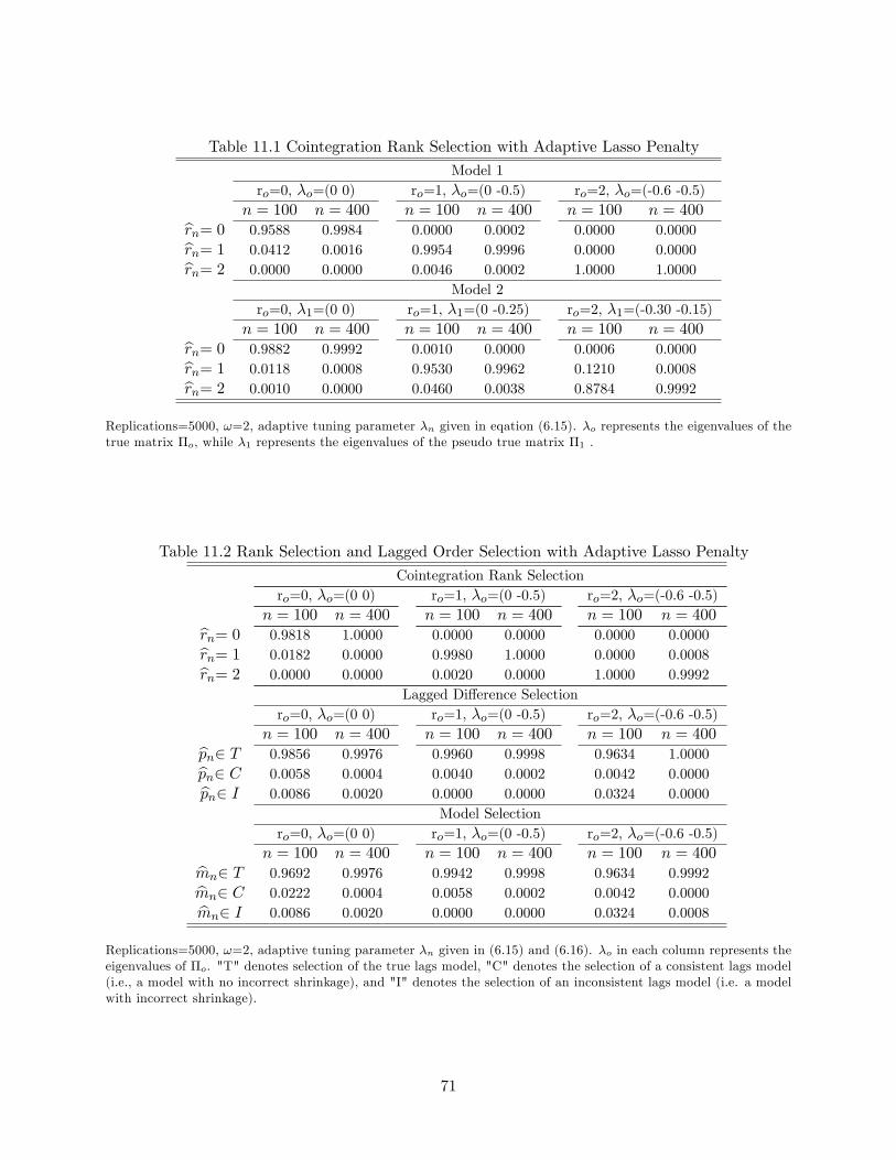
Table 11.1 Cointegration Rank Selection with Adaptive Lasso Penalty

Model 1ro=0, �o=(0 0) ro=1, �o=(0 -0.5) ro=2, �o=(-0.6 -0.5)

n = 100 n = 400 n = 100 n = 400 n = 100 n = 400brn= 0 0.9588 0.9984 0.0000 0.0002 0.0000 0.0000brn= 1 0.0412 0.0016 0.9954 0.9996 0.0000 0.0000brn= 2 0.0000 0.0000 0.0046 0.0002 1.0000 1.0000Model 2

ro=0, �1=(0 0) ro=1, �1=(0 -0.25) ro=2, �1=(-0.30 -0.15)n = 100 n = 400 n = 100 n = 400 n = 100 n = 400brn= 0 0.9882 0.9992 0.0010 0.0000 0.0006 0.0000brn= 1 0.0118 0.0008 0.9530 0.9962 0.1210 0.0008brn= 2 0.0010 0.0000 0.0460 0.0038 0.8784 0.9992

Replications=5000, !=2, adaptive tuning parameter �n given in eqation (6.15). �o represents the eigenvalues of thetrue matrix �o, while �1 represents the eigenvalues of the pseudo true matrix �1 .

Table 11.2 Rank Selection and Lagged Order Selection with Adaptive Lasso Penalty

Cointegration Rank Selectionro=0, �o=(0 0) ro=1, �o=(0 -0.5) ro=2, �o=(-0.6 -0.5)

n = 100 n = 400 n = 100 n = 400 n = 100 n = 400brn= 0 0.9818 1.0000 0.0000 0.0000 0.0000 0.0000brn= 1 0.0182 0.0000 0.9980 1.0000 0.0000 0.0008brn= 2 0.0000 0.0000 0.0020 0.0000 1.0000 0.9992Lagged Di¤erence Selection

ro=0, �o=(0 0) ro=1, �o=(0 -0.5) ro=2, �o=(-0.6 -0.5)n = 100 n = 400 n = 100 n = 400 n = 100 n = 400bpn2 T 0.9856 0.9976 0.9960 0.9998 0.9634 1.0000bpn2 C 0.0058 0.0004 0.0040 0.0002 0.0042 0.0000bpn2 I 0.0086 0.0020 0.0000 0.0000 0.0324 0.0000

Model Selectionro=0, �o=(0 0) ro=1, �o=(0 -0.5) ro=2, �o=(-0.6 -0.5)

n = 100 n = 400 n = 100 n = 400 n = 100 n = 400bmn2 T 0.9692 0.9976 0.9942 0.9998 0.9634 0.9992bmn2 C 0.0222 0.0004 0.0058 0.0002 0.0042 0.0000bmn2 I 0.0086 0.0020 0.0000 0.0000 0.0324 0.0008

Replications=5000, !=2, adaptive tuning parameter �n given in (6.15) and (6.16). �o in each column represents theeigenvalues of �o. "T" denotes selection of the true lags model, "C" denotes the selection of a consistent lags model(i.e., a model with no incorrect shrinkage), and "I" denotes the selection of an inconsistent lags model (i.e. a modelwith incorrect shrinkage).

71

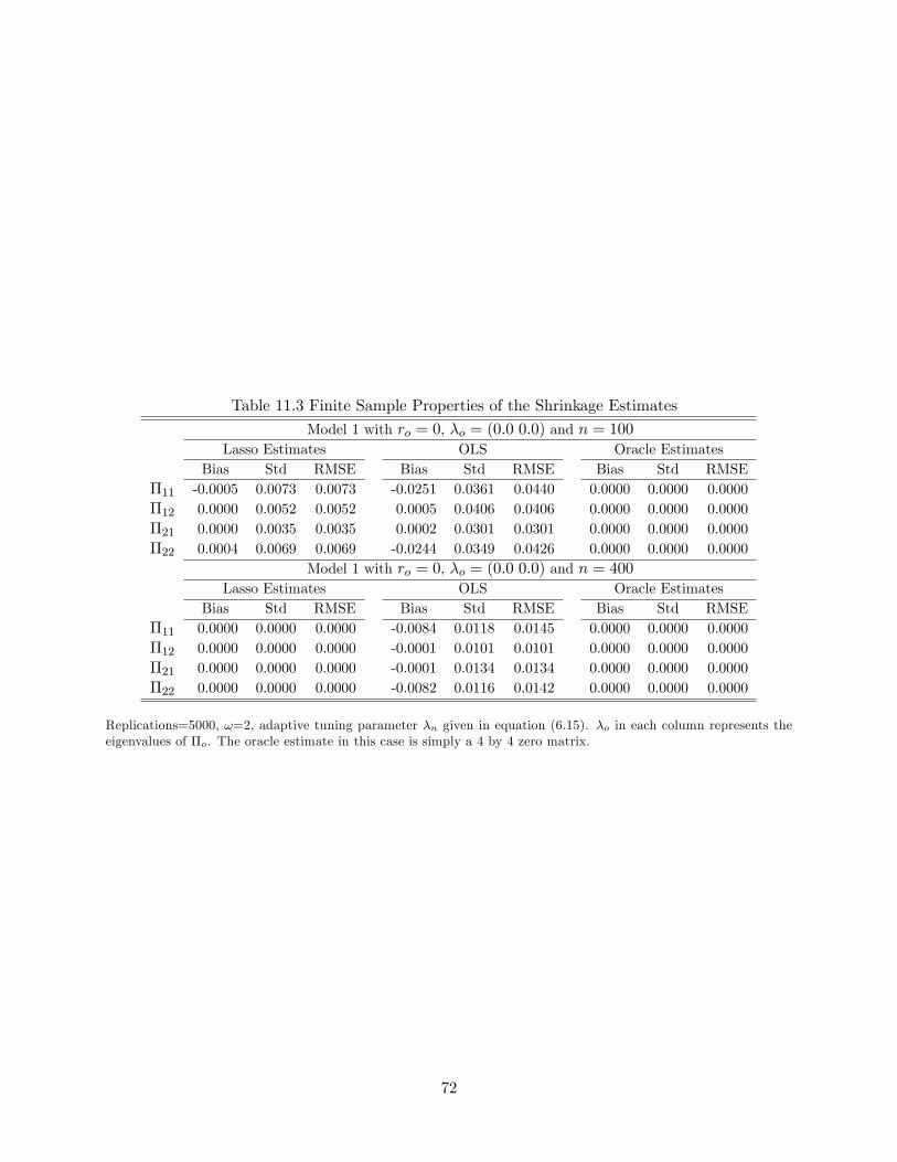
Table 11.3 Finite Sample Properties of the Shrinkage Estimates

Model 1 with ro = 0, �o = (0:0 0:0) and n = 100Lasso Estimates OLS Oracle Estimates

Bias Std RMSE Bias Std RMSE Bias Std RMSE�11 -0.0005 0.0073 0.0073 -0.0251 0.0361 0.0440 0.0000 0.0000 0.0000�12 0.0000 0.0052 0.0052 0.0005 0.0406 0.0406 0.0000 0.0000 0.0000�21 0.0000 0.0035 0.0035 0.0002 0.0301 0.0301 0.0000 0.0000 0.0000�22 0.0004 0.0069 0.0069 -0.0244 0.0349 0.0426 0.0000 0.0000 0.0000

Model 1 with ro = 0, �o = (0:0 0:0) and n = 400Lasso Estimates OLS Oracle Estimates

Bias Std RMSE Bias Std RMSE Bias Std RMSE�11 0.0000 0.0000 0.0000 -0.0084 0.0118 0.0145 0.0000 0.0000 0.0000�12 0.0000 0.0000 0.0000 -0.0001 0.0101 0.0101 0.0000 0.0000 0.0000�21 0.0000 0.0000 0.0000 -0.0001 0.0134 0.0134 0.0000 0.0000 0.0000�22 0.0000 0.0000 0.0000 -0.0082 0.0116 0.0142 0.0000 0.0000 0.0000

Replications=5000, !=2, adaptive tuning parameter �n given in equation (6.15). �o in each column represents theeigenvalues of �o. The oracle estimate in this case is simply a 4 by 4 zero matrix.

72

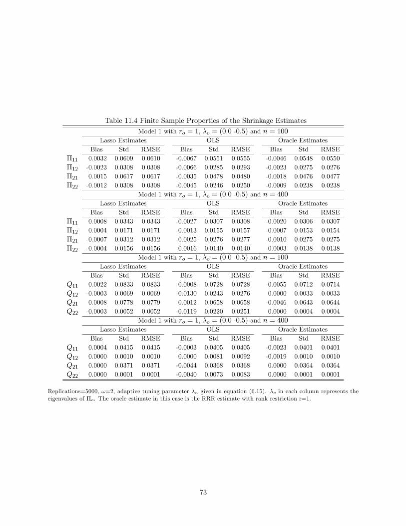
Table 11.4 Finite Sample Properties of the Shrinkage Estimates

Model 1 with ro = 1, �o = (0:0 -0:5) and n = 100Lasso Estimates OLS Oracle Estimates

Bias Std RMSE Bias Std RMSE Bias Std RMSE�11 0.0032 0.0609 0.0610 -0.0067 0.0551 0.0555 -0.0046 0.0548 0.0550�12 -0.0023 0.0308 0.0308 -0.0066 0.0285 0.0293 -0.0023 0.0275 0.0276�21 0.0015 0.0617 0.0617 -0.0035 0.0478 0.0480 -0.0018 0.0476 0.0477�22 -0.0012 0.0308 0.0308 -0.0045 0.0246 0.0250 -0.0009 0.0238 0.0238

Model 1 with ro = 1, �o = (0:0 -0:5) and n = 400Lasso Estimates OLS Oracle Estimates

Bias Std RMSE Bias Std RMSE Bias Std RMSE�11 0.0008 0.0343 0.0343 -0.0027 0.0307 0.0308 -0.0020 0.0306 0.0307�12 0.0004 0.0171 0.0171 -0.0013 0.0155 0.0157 -0.0007 0.0153 0.0154�21 -0.0007 0.0312 0.0312 -0.0025 0.0276 0.0277 -0.0010 0.0275 0.0275�22 -0.0004 0.0156 0.0156 -0.0016 0.0140 0.0140 -0.0003 0.0138 0.0138

Model 1 with ro = 1, �o = (0:0 -0:5) and n = 100Lasso Estimates OLS Oracle Estimates

Bias Std RMSE Bias Std RMSE Bias Std RMSEQ11 0.0022 0.0833 0.0833 0.0008 0.0728 0.0728 -0.0055 0.0712 0.0714Q12 -0.0003 0.0069 0.0069 -0.0130 0.0243 0.0276 0.0000 0.0033 0.0033Q21 0.0008 0.0778 0.0779 0.0012 0.0658 0.0658 -0.0046 0.0643 0.0644Q22 -0.0003 0.0052 0.0052 -0.0119 0.0220 0.0251 0.0000 0.0004 0.0004

Model 1 with ro = 1, �o = (0:0 -0:5) and n = 400Lasso Estimates OLS Oracle Estimates

Bias Std RMSE Bias Std RMSE Bias Std RMSEQ11 0.0004 0.0415 0.0415 -0.0003 0.0405 0.0405 -0.0023 0.0401 0.0401Q12 0.0000 0.0010 0.0010 0.0000 0.0081 0.0092 -0.0019 0.0010 0.0010Q21 0.0000 0.0371 0.0371 -0.0044 0.0368 0.0368 0.0000 0.0364 0.0364Q22 0.0000 0.0001 0.0001 -0.0040 0.0073 0.0083 0.0000 0.0001 0.0001

Replications=5000, !=2, adaptive tuning parameter �n given in equation (6.15). �o in each column represents theeigenvalues of �o. The oracle estimate in this case is the RRR estimate with rank restriction r=1.

73

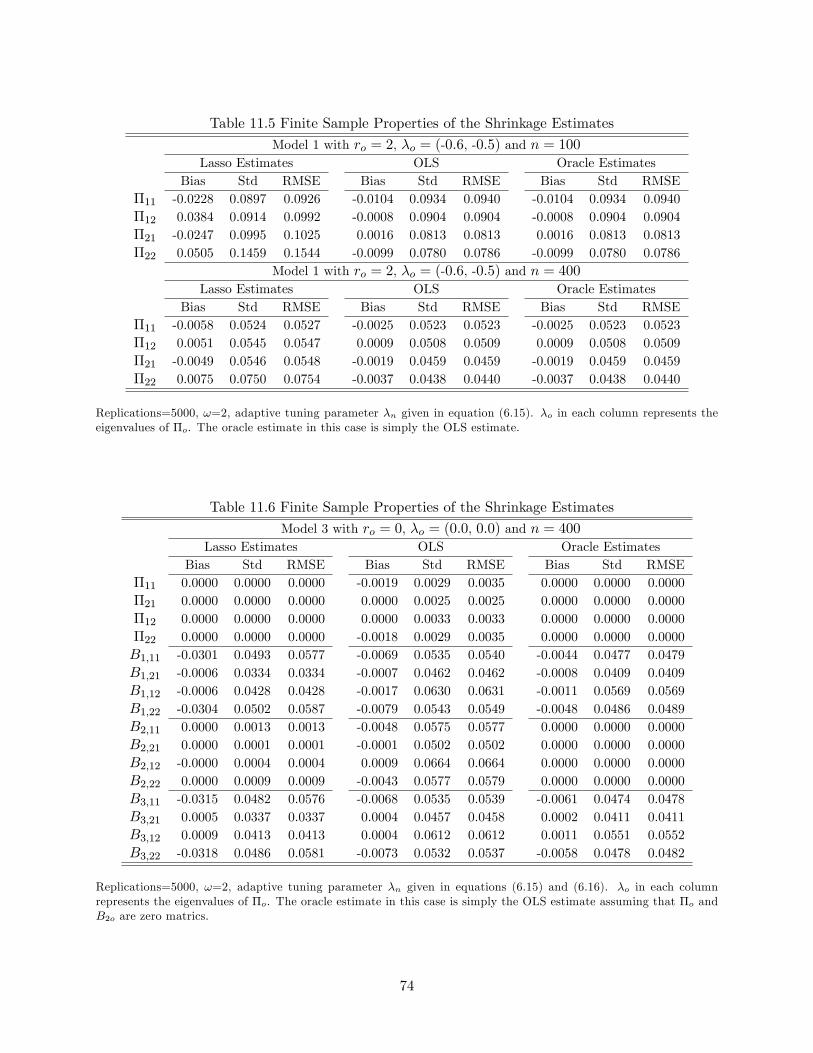
Table 11.5 Finite Sample Properties of the Shrinkage Estimates

Model 1 with ro = 2, �o = (-0:6, -0:5) and n = 100Lasso Estimates OLS Oracle Estimates

Bias Std RMSE Bias Std RMSE Bias Std RMSE�11 -0.0228 0.0897 0.0926 -0.0104 0.0934 0.0940 -0.0104 0.0934 0.0940�12 0.0384 0.0914 0.0992 -0.0008 0.0904 0.0904 -0.0008 0.0904 0.0904�21 -0.0247 0.0995 0.1025 0.0016 0.0813 0.0813 0.0016 0.0813 0.0813�22 0.0505 0.1459 0.1544 -0.0099 0.0780 0.0786 -0.0099 0.0780 0.0786

Model 1 with ro = 2, �o = (-0:6, -0:5) and n = 400Lasso Estimates OLS Oracle Estimates

Bias Std RMSE Bias Std RMSE Bias Std RMSE�11 -0.0058 0.0524 0.0527 -0.0025 0.0523 0.0523 -0.0025 0.0523 0.0523�12 0.0051 0.0545 0.0547 0.0009 0.0508 0.0509 0.0009 0.0508 0.0509�21 -0.0049 0.0546 0.0548 -0.0019 0.0459 0.0459 -0.0019 0.0459 0.0459�22 0.0075 0.0750 0.0754 -0.0037 0.0438 0.0440 -0.0037 0.0438 0.0440

Replications=5000, !=2, adaptive tuning parameter �n given in equation (6.15). �o in each column represents theeigenvalues of �o. The oracle estimate in this case is simply the OLS estimate.

Table 11.6 Finite Sample Properties of the Shrinkage Estimates

Model 3 with ro = 0, �o = (0:0, 0:0) and n = 400Lasso Estimates OLS Oracle Estimates

Bias Std RMSE Bias Std RMSE Bias Std RMSE�11 0.0000 0.0000 0.0000 -0.0019 0.0029 0.0035 0.0000 0.0000 0.0000�21 0.0000 0.0000 0.0000 0.0000 0.0025 0.0025 0.0000 0.0000 0.0000�12 0.0000 0.0000 0.0000 0.0000 0.0033 0.0033 0.0000 0.0000 0.0000�22 0.0000 0.0000 0.0000 -0.0018 0.0029 0.0035 0.0000 0.0000 0.0000B1;11 -0.0301 0.0493 0.0577 -0.0069 0.0535 0.0540 -0.0044 0.0477 0.0479B1;21 -0.0006 0.0334 0.0334 -0.0007 0.0462 0.0462 -0.0008 0.0409 0.0409B1;12 -0.0006 0.0428 0.0428 -0.0017 0.0630 0.0631 -0.0011 0.0569 0.0569B1;22 -0.0304 0.0502 0.0587 -0.0079 0.0543 0.0549 -0.0048 0.0486 0.0489B2;11 0.0000 0.0013 0.0013 -0.0048 0.0575 0.0577 0.0000 0.0000 0.0000B2;21 0.0000 0.0001 0.0001 -0.0001 0.0502 0.0502 0.0000 0.0000 0.0000B2;12 -0.0000 0.0004 0.0004 0.0009 0.0664 0.0664 0.0000 0.0000 0.0000B2;22 0.0000 0.0009 0.0009 -0.0043 0.0577 0.0579 0.0000 0.0000 0.0000B3;11 -0.0315 0.0482 0.0576 -0.0068 0.0535 0.0539 -0.0061 0.0474 0.0478B3;21 0.0005 0.0337 0.0337 0.0004 0.0457 0.0458 0.0002 0.0411 0.0411B3;12 0.0009 0.0413 0.0413 0.0004 0.0612 0.0612 0.0011 0.0551 0.0552B3;22 -0.0318 0.0486 0.0581 -0.0073 0.0532 0.0537 -0.0058 0.0478 0.0482

Replications=5000, !=2, adaptive tuning parameter �n given in equations (6.15) and (6.16). �o in each columnrepresents the eigenvalues of �o. The oracle estimate in this case is simply the OLS estimate assuming that �o andB2o are zero matrics.

74

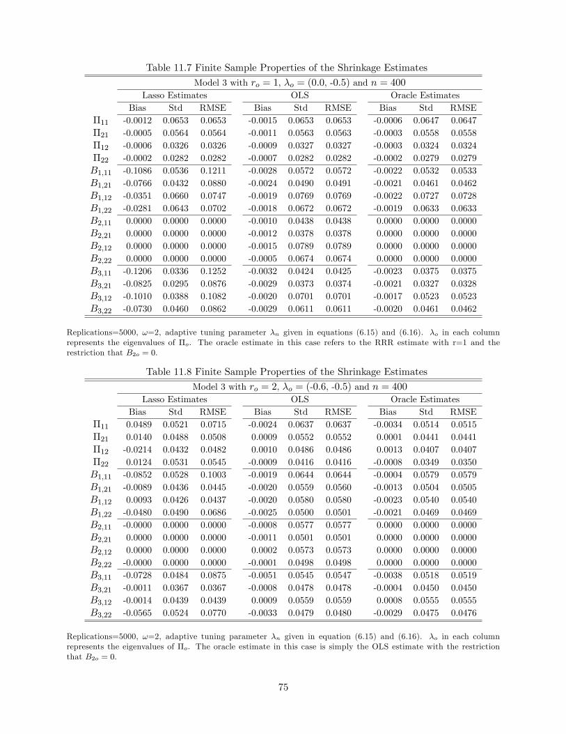
Table 11.7 Finite Sample Properties of the Shrinkage Estimates

Model 3 with ro = 1, �o = (0:0, -0:5) and n = 400Lasso Estimates OLS Oracle Estimates

Bias Std RMSE Bias Std RMSE Bias Std RMSE�11 -0.0012 0.0653 0.0653 -0.0015 0.0653 0.0653 -0.0006 0.0647 0.0647�21 -0.0005 0.0564 0.0564 -0.0011 0.0563 0.0563 -0.0003 0.0558 0.0558�12 -0.0006 0.0326 0.0326 -0.0009 0.0327 0.0327 -0.0003 0.0324 0.0324�22 -0.0002 0.0282 0.0282 -0.0007 0.0282 0.0282 -0.0002 0.0279 0.0279B1;11 -0.1086 0.0536 0.1211 -0.0028 0.0572 0.0572 -0.0022 0.0532 0.0533B1;21 -0.0766 0.0432 0.0880 -0.0024 0.0490 0.0491 -0.0021 0.0461 0.0462B1;12 -0.0351 0.0660 0.0747 -0.0019 0.0769 0.0769 -0.0022 0.0727 0.0728B1;22 -0.0281 0.0643 0.0702 -0.0018 0.0672 0.0672 -0.0019 0.0633 0.0633B2;11 0.0000 0.0000 0.0000 -0.0010 0.0438 0.0438 0.0000 0.0000 0.0000B2;21 0.0000 0.0000 0.0000 -0.0012 0.0378 0.0378 0.0000 0.0000 0.0000B2;12 0.0000 0.0000 0.0000 -0.0015 0.0789 0.0789 0.0000 0.0000 0.0000B2;22 0.0000 0.0000 0.0000 -0.0005 0.0674 0.0674 0.0000 0.0000 0.0000B3;11 -0.1206 0.0336 0.1252 -0.0032 0.0424 0.0425 -0.0023 0.0375 0.0375B3;21 -0.0825 0.0295 0.0876 -0.0029 0.0373 0.0374 -0.0021 0.0327 0.0328B3;12 -0.1010 0.0388 0.1082 -0.0020 0.0701 0.0701 -0.0017 0.0523 0.0523B3;22 -0.0730 0.0460 0.0862 -0.0029 0.0611 0.0611 -0.0020 0.0461 0.0462

Replications=5000, !=2, adaptive tuning parameter �n given in equations (6.15) and (6.16). �o in each columnrepresents the eigenvalues of �o. The oracle estimate in this case refers to the RRR estimate with r=1 and therestriction that B2o = 0.

Table 11.8 Finite Sample Properties of the Shrinkage Estimates

Model 3 with ro = 2, �o = (-0:6, -0:5) and n = 400Lasso Estimates OLS Oracle Estimates

Bias Std RMSE Bias Std RMSE Bias Std RMSE�11 0.0489 0.0521 0.0715 -0.0024 0.0637 0.0637 -0.0034 0.0514 0.0515�21 0.0140 0.0488 0.0508 0.0009 0.0552 0.0552 0.0001 0.0441 0.0441�12 -0.0214 0.0432 0.0482 0.0010 0.0486 0.0486 0.0013 0.0407 0.0407�22 0.0124 0.0531 0.0545 -0.0009 0.0416 0.0416 -0.0008 0.0349 0.0350B1;11 -0.0852 0.0528 0.1003 -0.0019 0.0644 0.0644 -0.0004 0.0579 0.0579B1;21 -0.0089 0.0436 0.0445 -0.0020 0.0559 0.0560 -0.0013 0.0504 0.0505B1;12 0.0093 0.0426 0.0437 -0.0020 0.0580 0.0580 -0.0023 0.0540 0.0540B1;22 -0.0480 0.0490 0.0686 -0.0025 0.0500 0.0501 -0.0021 0.0469 0.0469B2;11 -0.0000 0.0000 0.0000 -0.0008 0.0577 0.0577 0.0000 0.0000 0.0000B2;21 0.0000 0.0000 0.0000 -0.0011 0.0501 0.0501 0.0000 0.0000 0.0000B2;12 0.0000 0.0000 0.0000 0.0002 0.0573 0.0573 0.0000 0.0000 0.0000B2;22 -0.0000 0.0000 0.0000 -0.0001 0.0498 0.0498 0.0000 0.0000 0.0000B3;11 -0.0728 0.0484 0.0875 -0.0051 0.0545 0.0547 -0.0038 0.0518 0.0519B3;21 -0.0011 0.0367 0.0367 -0.0008 0.0478 0.0478 -0.0004 0.0450 0.0450B3;12 -0.0014 0.0439 0.0439 0.0009 0.0559 0.0559 0.0008 0.0555 0.0555B3;22 -0.0565 0.0524 0.0770 -0.0033 0.0479 0.0480 -0.0029 0.0475 0.0476

Replications=5000, !=2, adaptive tuning parameter �n given in equation (6.15) and (6.16). �o in each columnrepresents the eigenvalues of �o. The oracle estimate in this case is simply the OLS estimate with the restrictionthat B2o = 0.

75