Automated Analysis of Spatial Grids: Introduction

L AK S H M AN @ O U . E D U

3. Data Structures for Image

Analysis

Different formulations

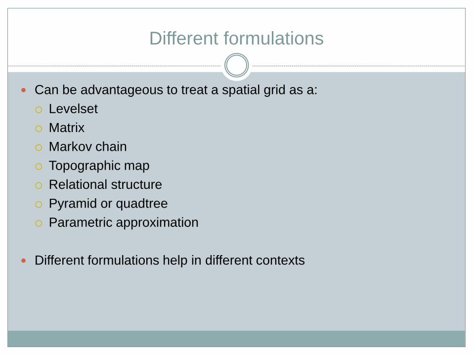
Can be advantageous to treat a spatial grid as a:

Levelset

Matrix

Markov chain

Topographic map

Relational structure

Pyramid or quadtree

Parametric approximation

Different formulations help in different contexts

Level set

Organizes the pixels in a grid by pixel value

Associative array

Between pixel value

And list of pixels that have that value

A “level” is a key-value pair

Could also use a random-access array if range is known

Creating a level set

To create a level set, traverse the grid once

How would you use the level set to find top 10 pixels?

Top 10 using a level set

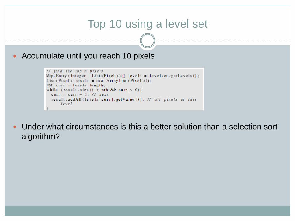
Accumulate until you reach 10 pixels

Under what circumstances is this a better solution than a selection sort

algorithm?

Topographic Grids

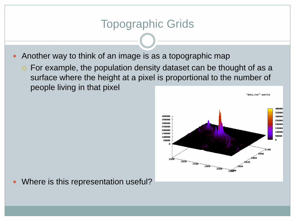
Another way to think of an image is as a topographic map

For example, the population density dataset can be thought of as a

surface where the height at a pixel is proportional to the number of

people living in that pixel

Where is this representation useful?

Thresholding

Thresholding an image implicitly treats the image topographically

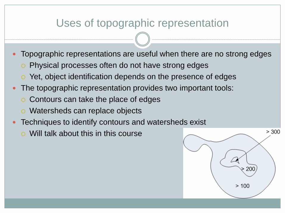
Uses of topographic representation

Topographic representations are useful when there are no strong edges

Physical processes often do not have strong edges

Yet, object identification depends on the presence of edges

The topographic representation provides two important tools:

Contours can take the place of edges

Watersheds can replace objects

Techniques to identify contours and watersheds exist

Will talk about this in this course

Topographic distances

You might want to consider distances taking into account topography

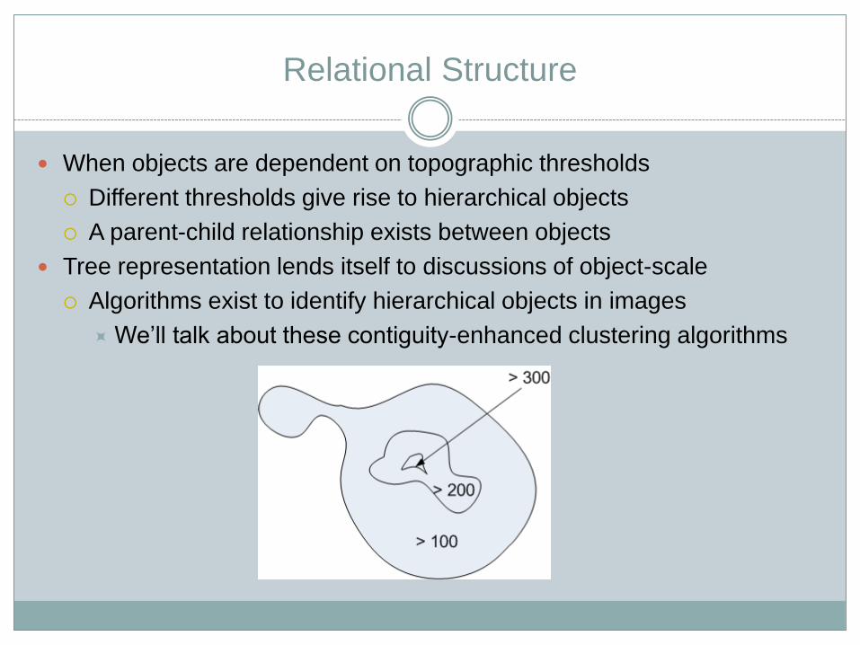
Relational Structure

When objects are dependent on topographic thresholds

Different thresholds give rise to hierarchical objects

A parent-child relationship exists between objects

Tree representation lends itself to discussions of object-scale

Algorithms exist to identify hierarchical objects in images

We’ll talk about these contiguity-enhanced clustering algorithms

Markov Chain

What’s a 1st order Markov Random Field?

A field where the value at x_k depends on x_{k-1} but not on x_{k-2},

etc. other than indirectly

Spatial dependence is of the 1st order only

Greatly simplifies many image processing operations if we assume

that the grid follows Markov properties

Enough to just consider the neighbors of a pixel

In most of this course, we’ll assume that your spatial grids were formed

by a 1st order Markov process

Rationale behind many of the techniques that we’ll discuss

What’s not Markov?

Your data are not Markov if:

You have gaps within your grid

Have to fill in (interpolate) the gaps before applying any image processing technique

You have speckle noise in your data

Speckle is uncorrelated with neighboring points

Need to speckle-filter your data first

Most common speckle filter: a median filter

Second order effects predominate in your data

Such as shadows caused by overshooting tops in satellite visible imagery

Remember that most image processing operations assume Markov

Think carefully about where the Markov assumption fails and fix them before doing any automated analysis

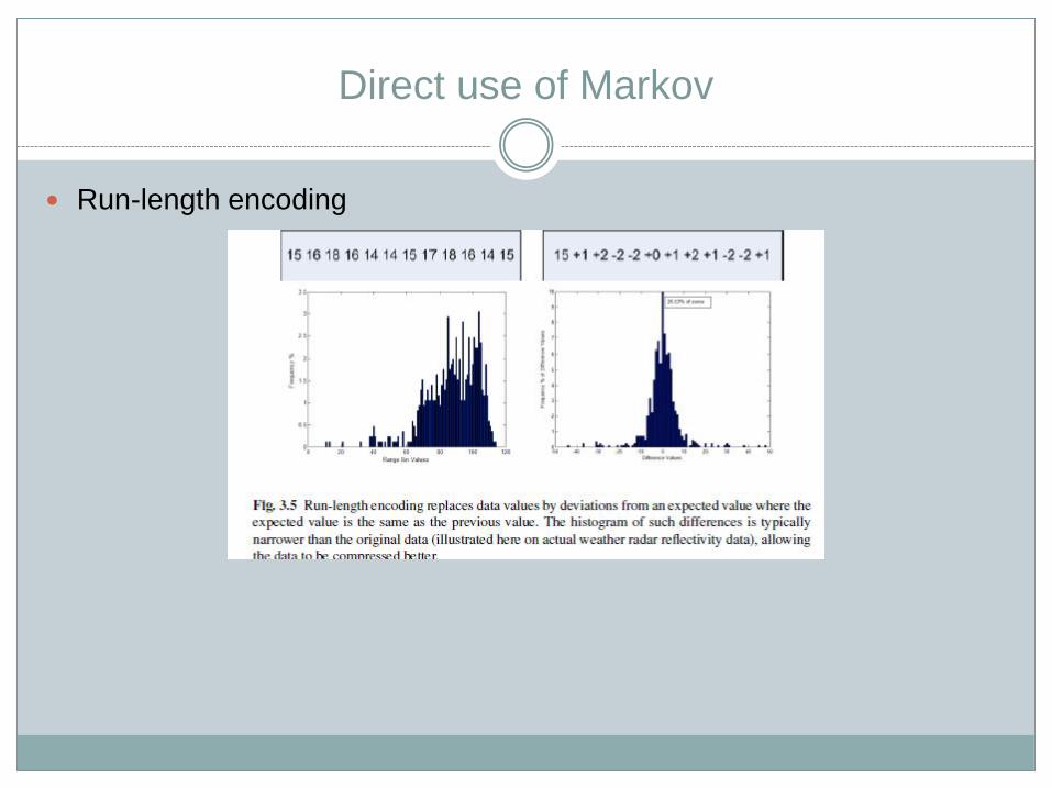
Direct use of Markov

Run-length encoding

Matrix formulation

Can think of a spatial grid as a matrix X

Useful for simple scalar operations built into statistical packages

max(X), sumRows(X), etc.

Any other use for matrix notation?

Matrix formulation

Recall that in objective analysis the resulting value at a grid point is the

weighted average of the inputs

Can think of the resulting grid as

X = a1 X1 + a2 X2 + … + an Xn

The left-hand-side “X” is the final image as a matrix

What does Xk look like?

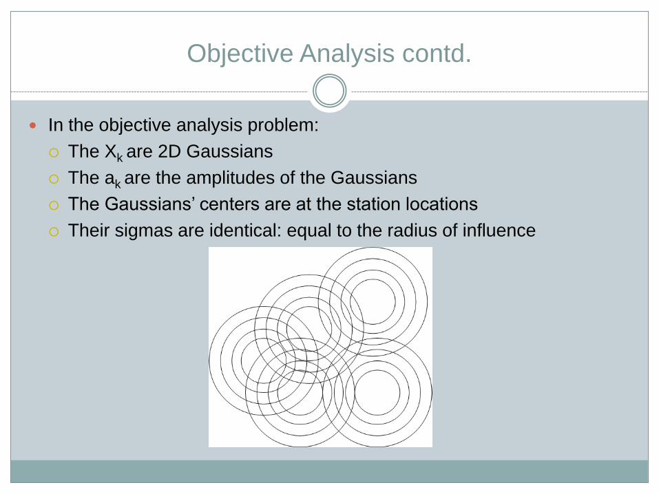
Objective Analysis contd.

In the objective analysis problem:

The Xk are 2D Gaussians

The ak are the amplitudes of the Gaussians

The Gaussians’ centers are at the station locations

Their sigmas are identical: equal to the radius of influence

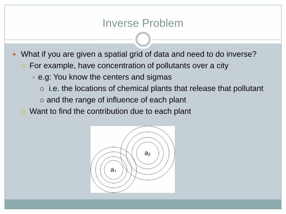
Inverse Problem

What if you are given a spatial grid of data and need to do inverse?

For example, have concentration of pollutants over a city

e.g: You know the centers and sigmas

i.e. the locations of chemical plants that release that pollutant

and the range of influence of each plant

Want to find the contribution due to each plant

Radial Basis Functions

Can treat the X’s as basis functions

X = a1 X1 + a2 X2 + … + an Xn

The final grid is then a linear combination of Radial Basis Functions

If the X’s are known, the least-squares optimal amplitudes can be found

using singular value decomposition

RBF Formulation

Treat the result image (‘y’) as a matrix with p rows and 1 column

p is the number of pixels in the image

The 2D Gaussian function (x is a 2x1 vector)

h(x) = exp(-(x-c)T(x-c)/r2)

The center and r of each Gaussian is known

y at the row corresponding to x = [ a1h1(x) + … + amhm(x) ]

m is the number of Gaussians

The optimal amplitudes to minimize the least squares error is:

a = (HTH)-1 HT y

Introduction to Radial Basis Function Networks by MJL Orr

Do a Google search and download from psu.edu

Read pages 6-12 in order to do assignment

Parametric Approximation

If you identify objects using the topographic formulation, you throw

away data outside the peaks

The data corresponding to low values do not form part of the object

Can approximate an image by a 2D function

The RBF was an attempt at doing this

But limited to Gaussians of known centers and sigmas

Not all that applicable

Gamma functions and Gaussian Mixture Models are more flexible

Parametric approximations permit some interesting forms of analyses

Will look at ways to do the approximation and what can be achieved

with those

Assignment Part 1: Radial Basis Functions

Simulate and solve the 2-source pollutant problem:

Simulate a spatial grid by objectively analyzing two point sources

Starting with the known locations and sigmas, determine the

amplitude of the Gaussians using RBFs

How close do you get?

Extra credit: How does this change with noise?

Extending a RBF

Can you think of a spatial inverse problem where a RBF can be used?

Recall that the RBF has an optimal solution only if you know the

centers and sigmas apriori

Will the centers and sigmas be known apriori?

How could you address this issue?

Projection Pursuit

An iterative procedure that is not optimal, but usually “good enough”

Find centers and sigmas one-by-one

1. Find first center and sigma

2. Compute amplitude of the RBFs

3. Compute image approximation from RBF and compute error

4. If error > error-threshold or number-of-RBF < max-no-of-RBF

Find next center and sigma; Add to list of centers and sigmas

Go to step 2

How to find a “good-enough” center and sigma?

Could find spatial mean (centroid) and spatial variance

Or use peak of error code to locate center and use distance from peak to half-its-value to come up with a variance estimate

Better approach since RBFs are “local” estimators

Projection Pursuit on Simulated Input

RBF#0 center: [24,32 20] sigmax=6.0 sigmay=10.0




true RBF#0 center: [25,33 20] sigmax=8.0 sigmay=12.0

true RBF#1 center: [33,50 10] sigmax=12.0 sigmay=8.0

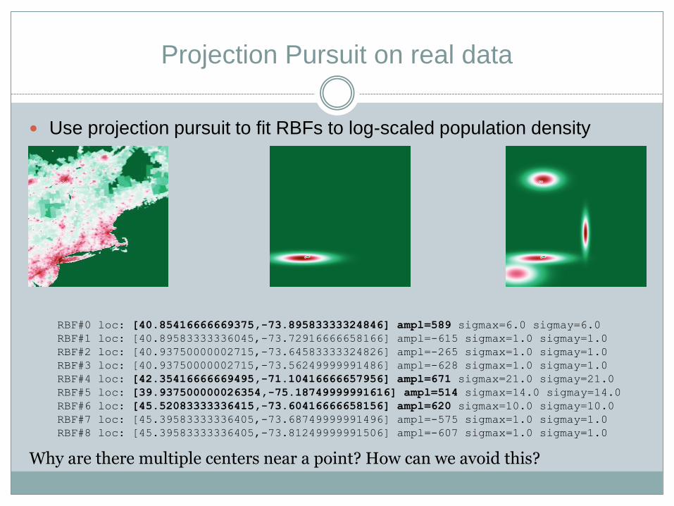
Projection Pursuit on real data

Use projection pursuit to fit RBFs to log-scaled population density

RBF#0 loc: [40.85416666669375,-73.89583333324846] ampl=589 sigmax=6.0 sigmay=6.0

RBF#1 loc: [40.89583333336045,-73.72916666658166] ampl=-615 sigmax=1.0 sigmay=1.0








Why are there multiple centers near a point? How can we avoid this?

Assignment Part 2: Top 5 population centers

Find the top 5 population centers in North America

Mark the approximate metropolitan area of each

Parametric approximation

RBF:

Have to know centers and sigmas

Projection pursuit:

Heuristic ways to choose centers and amplitudes

Tends to put centers displaced from true values

Because first center is a “’weighted average”

Gaussian Mixture Model

Parametric approximation of a spatial grid

Gaussian Mixture Model

GMM => Probability

The GMM scaling has been chosen to add up to 1

Images will not sum up to one

But you can normalize the image so that it does

Then, approximate it with a GMM

Procedure to approximate a GMM is expectation-minimization

What is EM?

Do you know any EM procedure?

GMM E-step

Assume an initial choice of parameters

Then, compute the likelihood of the set of parameters (E step)

GMM M-step

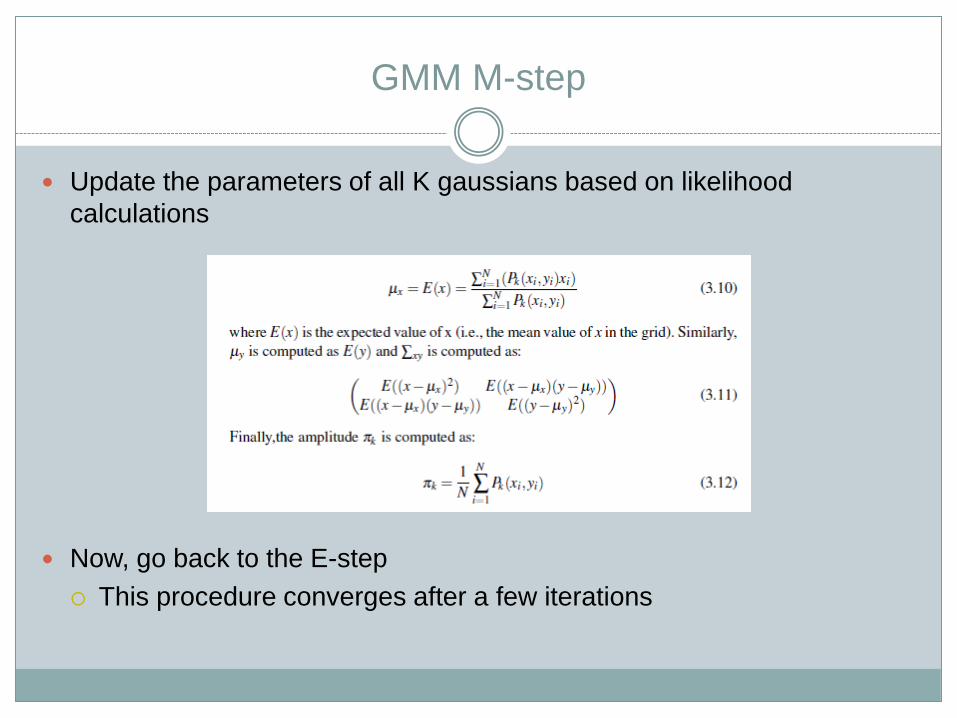
Update the parameters of all K gaussians based on likelihood

calculations

Now, go back to the E-step

This procedure converges after a few iterations

GMM considerations: stopping

How do we stop?

Look for improvement to be less than some threshold

Use GMM to approximate spatial grid

Computer error and stop when error falls below threshold

Problem: our threshold may be unrealistic for our K value

More common: look for percent improvement to be below

threshold (from iteration to next iteration)

Common to define improvement based on log(likelihood) as error

measure

GMM consideration: initializing

How do we initialize GMM?

The number of Gaussians?

The initial means of the Gaussians?

Could start from level set and top N pixels as long as these are

spaced reasonably far apart

Note that the GMM (unlike RBF) will move the centers

Not stuck with these centers

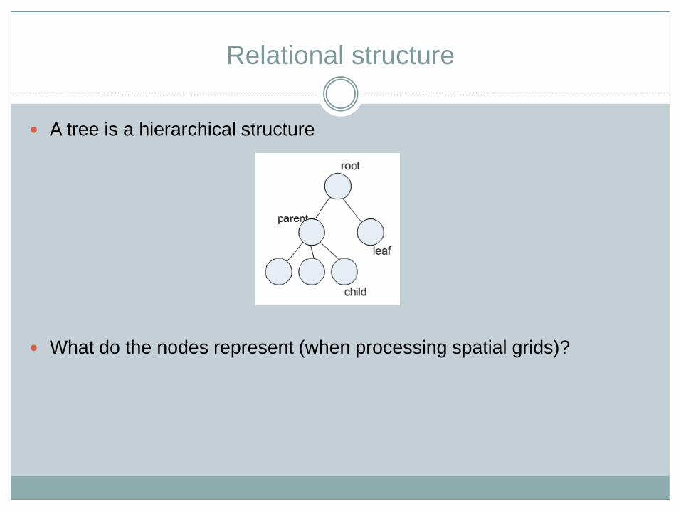
Relational structure

A tree is a hierarchical structure

What do the nodes represent (when processing spatial grids)?

Nodes in tree

Nodes could represent:

Objects

Multi-scale approaches

Objects at different sizes

Coarser resolution spatial grids

Multi-resolution approaches

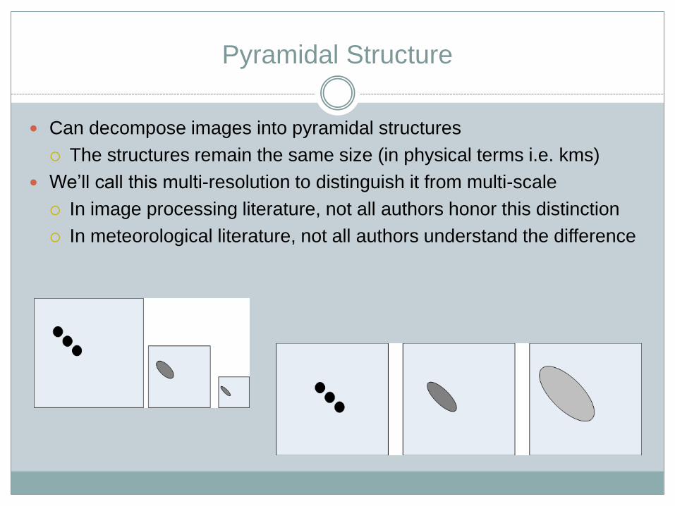
Pyramidal Structure

Can decompose images into pyramidal structures

The structures remain the same size (in physical terms i.e. kms)

We’ll call this multi-resolution to distinguish it from multi-scale

In image processing literature, not all authors honor this distinction

In meteorological literature, not all authors understand the difference

Wavelets and Multi-resolution

Can be advantageous to be able to reconstruct an image from the

pyramid decomposition of the image

Smoothing the image with Gaussians of different scales and

resampling will not allow you to do this

Wavelets are special functions that give you this ability

Wavelets solve the multi-resolution reconstruction problem

Usually inappropriate to solve the multi-scale problem!

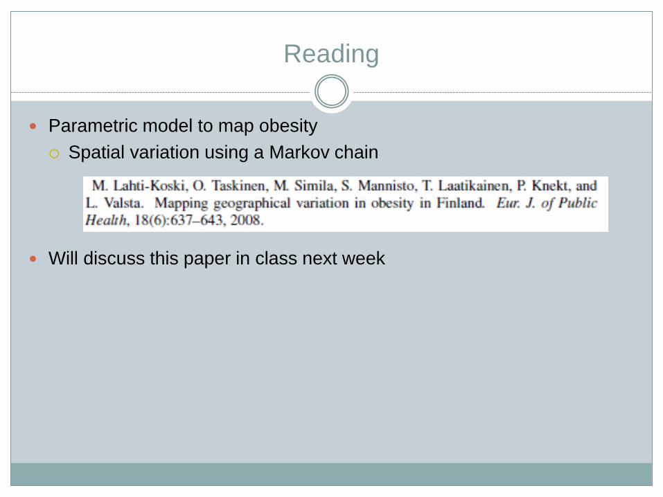
Reading

Parametric model to map obesity

Spatial variation using a Markov chain

Will discuss this paper in class next week

Automated Analysis of Spatial Grids: Introduction

Documents

Transcript of Automated Analysis of Spatial Grids: Introduction