AUTODEVS: A METHODOLOGY FOR AUTOMATING...
196
AUTODEVS: A METHODOLOGY FOR AUTOMATING SYSTEMS DEVELOPMENT by Manuel C. Salas _____________________________ Copyright © Manuel C. Salas 2008 A Thesis Submitted to the Faculty of the DEPARTMENT OF ELECTRICAL AND COMPUTER ENGINEERING In Partial Fulfillment of the Requirements For the Degree of MASTER OF SCIENCE WITH A MAJOR IN COMPUTER ENGINEERING In the Graduate College THE UNIVERSITY OF ARIZONA 2008
Transcript of AUTODEVS: A METHODOLOGY FOR AUTOMATING...

AUTODEVS: A METHODOLOGY FOR AUTOMATING SYSTEMS DEVELOPMENT
by
Manuel C. Salas
_____________________________ Copyright © Manuel C. Salas 2008
A Thesis Submitted to the Faculty of the
DEPARTMENT OF ELECTRICAL AND COMPUTER ENGINEERING
In Partial Fulfillment of the Requirements
For the Degree of
MASTER OF SCIENCE
WITH A MAJOR IN COMPUTER ENGINEERING
In the Graduate College
THE UNIVERSITY OF ARIZONA
2008

STATEMENT BY AUTHOR
This thesis has been submitted in partial fulfillment of requirements for an advanced degree at the University of Arizona and is deposited in the University Library to be made available to borrowers under rules of the Library.
Brief quotations from this thesis are allowable without special permission, provided that accurate acknowledgment of source is made. Requests for permission for extended quotation from or reproduction of this manuscript in whole or in part may be granted by the head of the major department or the Dean of the Graduate College when in his or her judgment the proposed use of the material is in the interests of scholarship. In all other instances, however, permission must be obtained from the author.
SIGNED: Manuel C. Salas
APPROVED BY THESIS DIRECTOR
This thesis has been approved on the date shown below: ________________________________ _____________________ Bernard P. Zeigler Date Professor of Electrical and Computer Engineering

ACKNOWLEDGEMENTS
I would like to thank my advisor Dr. Bernard Zeigler, for his support, encouragement, mentoring and invaluable guidance. He gave me the freedom to develop an original line of thinking and pursue independent ideas.
I express my thanks to the committee members Dr. Jonathan Sprinkle, and Dr. Salim Hariri for providing suggestions; enhancing the content of this thesis.
I would also like to express thanks to my colleagues at ACIMS lab, Chungman Seo, Dr. Saurabh Mittal, Ho Jun Lee and Xiaoyan Wei for helping out over the elaboration of my thesis.
Last but not least, my mother Graciela, my father Rene, my brother Rene and friends who stood by me during this endeavor. Many thanks to them for their continuous support, understanding and encouragement.

To my parents: Graciela Cardenas and Rene Salas
To my brother: Rene Salas

5
TABLE OF CONTENTS
LIST OF FIGURES..........................................................................8
LIST OF FIGURES - Continued......................................................9
LIST OF FIGURES - Continued....................................................10
LIST OF TABLES ......................................................................... 11
ABSTRACT................................................................................... 12
CHAPTER 1. INTRODUCTION............................................. 13
1.1 System Development ......................................................................................... 13
1.2 Modeling & Simulation Based Development .................................................... 17
1.3 Automatic Programming.................................................................................... 22
1.4 Real-Time Systems Development...................................................................... 23
1.5 Distributed Systems Development..................................................................... 26
1.6 M&S Development Tools .................................................................................. 28
1.7 Service Oriented Architecture............................................................................ 34
1.8 Summary of Contributions................................................................................. 37
1.9 Thesis Organization ........................................................................................... 38
CHAPTER 2. DISCRETE EVENT SYSTEM SPECIFICATION (DEVS)…………………………………………………………..40
2.1 DEVS Framework.............................................................................................. 40
2.2 DEVS Concepts Review .................................................................................... 43
2.3 Modeling Using DEVS ...................................................................................... 52
2.4 DEVS Activity ................................................................................................... 57
2.5 Simulation and Execution of DEVS Models ..................................................... 59
CHAPTER 3. DEVS & MODEL CONTINUITY....................63

6
TABLE OF CONTENTS - Continued
3.1 Model Continuity in Software Development ..................................................... 63
3.2 Modeling, Simulation, Execution, and Model Continuity ................................. 66
3.2.1 Model Continuity for Non-Distributed Real-time Systems ........................ 66
3.2.2 Model Continuity for Distributed Real-time Systems ................................ 70
3.3 Simulation-based Test for Real-time Systems ................................................... 73
3.3.1 A Virtual Test Environment........................................................................ 73
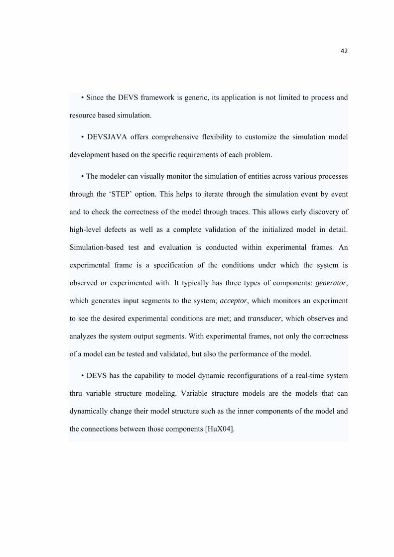
3.3.2 Incremental Simulation and Test for Non-Distributed Real-time System.. 74
3.3.3 Incremental Simulation and Test for Distributed Real-time Systems ........ 77
3.4 DEVS Development Process.............................................................................. 81
3.5 abstractActivity .................................................................................................. 84
CHAPTER 4. DEVS-BASED TOOLS ....................................87
4.1 SES & SESBuilder............................................................................................. 87
4.2 Finite Deterministic DEVS (FDDEVS) ............................................................. 95
4.2.1 Working with FD-DEVS GUI .................................................................... 99
4.3 DEVS/SOA ...................................................................................................... 105
CHAPTER 5. AUTODEVS ................................................... 111
5.1 Background ...................................................................................................... 111
5.2 Motivation ........................................................................................................ 114
5.3 General Description ......................................................................................... 115
5.4 AutoDEVS & Model Continuity...................................................................... 125
CHAPTER 6. AUTODEVS TO AUTONOMOUS ROAD SURVEY SYSTEM DEVELOPMENT....................................... 138
6.1 Autonomous Road Survey System................................................................... 138
6.2 ARS Process..................................................................................................... 140
6.3 Developing ARS Models using AutoDEVS .................................................... 146
6.3.1 CentralSystem........................................................................................... 153

7
TABLE OF CONTENTS - Continued
6.4 Adding more Behavior Aspects to the ARS Models ....................................... 167
6.5 Stepwise Simulation, Deployment, and Execution .......................................... 169
6.5.1 Central Simulation .................................................................................... 169
6.5.2 Distributed Simulation .............................................................................. 171
6.5.3 Deployment and Execution....................................................................... 175
6.5.4 Results and Discussions............................................................................ 175
CHAPTER 7. CONCLUSIONS AND FUTURE WORK...... 179
7.1 Conclusions ...................................................................................................... 179
7.2 Future Work ..................................................................................................... 183
APPENDIX A: Runner Artificial Intelligence............................. 186
APPENDIX B: CentralSystem Artificial Intelligence ................. 187
APPENDIX C: Data Structures used in ARS .............................. 189
APPENDIX D: DEVS/SOA Installation...................................... 190
REFERENCES............................................................................. 191

8
LIST OF FIGURES
Figure 1.1 SDLC Waterfall Model ................................................................................... 13 Figure 1.2 SDLC V-Shaped Model .................................................................................. 14 Figure 1.3 SDLC Incremental Model ............................................................................... 15 Figure 1.4 SDLC Spiral Model......................................................................................... 16 Figure 2.1 Basic Entities and Relations ............................................................................ 44 Figure 2.2 Discrete event time segments. ......................................................................... 45 Figure 2.3 Interpretation of DEVS structure..................................................................... 48 Figure 2.4 A “leader-follower” system modeled by a DEVS coupled model .................. 53 Figure 2.5 Timed state diagram of a screen saver program.............................................. 54 Figure 2.6 Time patterns modeled in DEVS..................................................................... 56 Figure 2.7 DEVS model, activity and the external environment...................................... 58 Figure 2.8 Simulate/Execute DEVS model in centralized and distributed environment.. 59 Figure 2.9 Hierarchical distributed simulation or execution topology ............................. 62 Figure 3.1 Modeling, Simulation and Execution of Non-distributed Real-time System.. 67 Figure 3.2 Modeling, Simulation and Execution of Distributed Real-time System ......... 71 Figure 3.3 Step-wise Simulations of Non-distributed Real-time System......................... 75 Figure 3.4 Simulation-based test of Distributed Real-time System.................................. 78 Figure 3.5Development Process of the Methodology....................................................... 82 Figure 3.6 Environment, models, activity, and abstractActivity ...................................... 85 Figure 4.1Mapping aspects to composite models ............................................................. 89 Figure 4.2 Mapping multiAspects to composite models .................................................. 90 Figure 4.3 Mapping multiAspects to composite models .................................................. 91 Figure 4.4 Interpreting multiple aspects as alternative decompositions ........................... 92 Figure 4.5 SESBuilder Natural Language View............................................................... 94 Figure 4.6 SESBuilder Tree View .................................................................................... 95 Figure 4.7 GUI to generate DEVS models ..................................................................... 100 Figure 4.8 Snapshot to consturct state-TimeAdvance pairs............................................ 101 Figure 4.9 Snapshot to construct internal behavior as Delta-int function....................... 102 Figure 4.10 Snapshot to construct external input behavior as Delta-ext function .......... 103 Figure 4.11 Snapshot showing generated XML FD-DEVS model for proc' .................. 104 Figure 4.12 Snapshot showing generated Java FD-DEVS model for 'proc' ................... 105 Figure 4.13 DEVS/SOA distributed architecture............................................................ 107 Figure 4.14 GUI snapshot of DEVS/SOA client hosting distributed simulation ........... 109 Figure 4.15 Server Assignment To Models .................................................................... 110 Figure 5.1 AutoDEVS Graphical User Interface ............................................................ 116

9
LIST OF FIGURES - Continued Figure 5.2 AutoDEVS: Requirements Specification ...................................................... 117 Figure 5.3 AutoDEVS: Automated PES......................................................................... 120 Figure 5.4 AutoDEVS: tree representation of the PES created. ..................................... 121 Figure 5.5 AutoDEVS: PES user selection..................................................................... 122 Figure 5.6 DEVSJAVA SimView running system under development ......................... 123 Figure 5.7 Agent Development Example: Define Requirements ................................... 126 Figure 5.8 Agent Development Example: Define Structural Aspects ............................ 127 Figure 5.9 Agent Development Example: Define Behavioral Aspects .......................... 128 Figure 5.10 Agent Development Example: Capture Spreadsheet Data.......................... 129 Figure 5.11 Agent Development Example: Generate FDDEVS .................................... 130 Figure 5.12 Agent Development Example: Generate MicroSESRepresentation ........... 131 Figure 5.13 Agent Development Example: SES Tree View........................................... 132 Figure 5.14 Agent Development Example: Choosing a PES ......................................... 133 Figure 5.15 Agent Development Example: Generate Test Models ................................ 134 Figure 5.16 Agent Development Example: Verifying models in SES, FDDEVS, and SimView ......................................................................................................................... 135 Figure 5.17 Agent Development Example: Running models in SimView..................... 136 Figure 5.18 AutoDEVS Life-Cycle Process ................................................................... 137 Figure 6.1Gold Mine in Canada...................................................................................... 139 Figure 6.2 AutonomousRoadSurvey Main Abstraction Components ............................ 141 Figure 6.3 ARS User Interface Map Generator .............................................................. 142 Figure 6.4 ARS Persistence Storage File........................................................................ 143 Figure 6.5 ARS 2D Cell Grid Plot .................................................................................. 144 Figure 6.6 ARS Report Generated by CentralSystem .................................................... 146 Figure 6.7 ARS Requirement Specifications .................................................................. 147 Figure 6.8 ARS Models Produced by AutoDEVS: Structural Aspects .......................... 149 Figure 6.9 ARS Models Produced by AutoDEVS: Behavioral Aspects ........................ 150 Figure 6.10 ARS PES Produced by AutoDEVS............................................................. 151 Figure 6.11 ARS SES Tree View produced by the AutoDEVS. .................................... 152 Figure 6.12 ARS CentralSystem Model ......................................................................... 153 Figure 6.13 CentralSystem State Diagram...................................................................... 154 Figure 6.14 WirelessAdapter State Diagram .................................................................. 156 Figure 6.15 ARS Runners Model.................................................................................... 157 Figure 6.16 Runner State Diagram ................................................................................. 158 Figure 6.17 GpsReceiver State Diagram ........................................................................ 159 Figure 6.18 SurfaceSensor State Diagram...................................................................... 160

10
LIST OF FIGURES - Continued Figure 6.19 ARS SurveyEF Model................................................................................. 161 Figure 6.20 SEFCoordinator State Diagram................................................................... 162 Figure 6.21 mapCoord State Diagram ............................................................................ 163 Figure 6.22 Abstract Activity Classes ............................................................................ 165 Figure 6.23 JobT_Transducer State Diagram ................................................................. 166 Figure 6.24 ARS Distributed Simulation........................................................................ 171 Figure 6.25 GUI snapshot of DEVSV/SOA client hosting distributed simulation......... 172 Figure 6.26 Assigning IP addresses to Models............................................................... 173 Figure 6.27 DEVS/SOA: ARS Distributed Simulation .................................................. 174 Figure 6.28 MineMap of study (left) and AutonomousRoadSurvey output (right)........ 175 Figure 6.29 MineMap II of study (left) and AutonomousRoadSurvey output (right). ... 176 Figure 6.30 MineMap III of study (left) and AutonomousRoadSurvey output (right)... 177

11
LIST OF TABLES
Table 4-1 Mapping SES elements to simulation model elements .................................... 88 Table 4-2 FDDEVS to DEVS mapping ............................................................................ 98 Table 5-1 Rules for Restricted NLP based Requirement Specifications ........................ 118

12
ABSTRACT
The need to improve productivity, quality and complexity hiding during systems
development has always been an important objective for the success of an organization.
The constant pressure to deliver systems within minimum time and reduced cost, the
rapid generation of prototypes to enhance testing and detect flaws at early stages, and the
need to reduce development cycles and growing design complexity without
compromising quality are challenges that organizations face when trying to be more
successful than their competitors.
Originally introduced as formalism for discrete event modeling and simulation,
the DEVS (Discrete Event System Specification) methodology has become an engine for
advances within the wider area of information technology.
In this work, a distributed simulation-based system for an autonomous robotic
survey is developed to show how this new DEVS-based tool called “AutoDEVS”
automates the systems development and exploits “model continuity” to maintain
coherence through the development process.

13
CHAPTER 1. INTRODUCTION
1.1 System Development
The objective of systems development is to find solutions to problems. These
problems may entail the development of simple or complex systems that involve software,
hardware, procedures and organizations. System development is typically accomplished
by using a set of systematic methodologies that divide large, complex tasks into smaller
and more easily managed phases, allowing management to elaborate more accurate plans,
verify the successful completion of a phase, and improve the allocation of resources for
subsequent phases.
Traditionally, many organizations make use of the Systems Development Life Cycle
(SDLC) methodology to assist in developing systems, as it ensures that all functional and
non-functional requirement goals and objectives are met. SDLC provides a set of models
or methodologies such as waterfall, v-shaped, incremental, spiral, build and fix, and
synchronize and stabilize. The waterfall model defines a sequence of stages in which the
output of each stage becomes the input for the next.
Figure 1.1 SDLC Waterfall Model

14
As seen in Figure 1.1, the waterfall model contains the following stages: project planning,
feasibility study, systems analysis, requirements definition, systems design,
implementation, integration and testing, acceptance, installation, deployment, and
maintenance [Wri08]. This model allows phases to be processed and completed one at a
time but it is very rigid and changes to requirements can potentially have a negative
impact on the system. The v-shaped model is similar to the waterfall model with the
difference that testing procedures are developed before starting the implementation phase,
see Figure 1.2.
Figure 1.2 SDLC V-Shaped Model
The V-shaped model has more probability for success than the waterfall model due to the
development of test plans early on during the life cycle process. On the other hand, no
early prototypes of the system are produced [Lew08]. As seen in Figure 1.3, the
incremental model consists of dividing the waterfall model into smaller, more easily
managed iterations.

15
Figure 1.3 SDLC Incremental Model
The incremental model allows having a base working version of the system, where flaws
are detected quickly and early in the process. On the other hand, system architecture
problems may arise due to changes in requirements in later iterations [Lew08]. The spiral
model is most often used in large, complex and expensive systems. This model is similar
to the incremental model, with more emphases on risk analysis.

16
Figure 1.4 SDLC Spiral Model
As seen in Figure 1.4, the spiral model includes high amount of risk analysis that allows
evaluating different alternatives to mitigate a specific problem and then choose the best
fit for the system in development. On the other hand, the project success is highly
dependent on the risk analysis phase. In the build and fix model a system is built with
minimal requirements and specifications, no design or testing is executed. The build and
fix model is usually effective in very small projects where the complexity is very limited.
However, maintenance could become an issue since no documentation is produced and
when this model is applied to highly-complex systems it can result in a low quality,
delayed and costly system [Lew08]. In the synchronize and stabilize model, teams work
concurrently on individual application modules, executing frequent code synchronization

17
between the teams, and allowing to stabilize the system regularly throughout the
development process. Since the synchronize and stabilize model allows changes at any
point throughout the process, it is inherently more flexible, and allows responsiveness to
changing business requirements.
There are alternatives to the SDLC models such as Joint Applications Design
(JAD) and Rapid Application Development (RAD). The JAD technique allows end users
to participate in the requirements development process to better understand their needs
and set up the desired system. When the size of the group and the system is too large, the
JAD technique could become expensive and cumbersome; however it reduces the
ambiguity produced during the system requirements elaboration phase [Woo95]. The
RAD model involves iterative development and construction of prototypes that allow
emulating and provide the ability to quickly build working systems to test their
usefulness. This model provides the ability to rapidly change system design as demanded
by users. Following the rapid prototyping model can lead to a succession of prototypes
that never culminate in a satisfactory production application [Mar91]. More speed and
lower cost may lead to lower overall quality. Potential for inconsistent designs within and
across systems and the difficulty with model reuse for future systems are some of the
most common weaknesses of the RAD model [Cms08].
1.2 Modeling & Simulation Based Development
Computer system users, administrators, and designers usually have a goal of highest
performance at lowest cost. Modeling and Simulation during system development is good

18
preparation for design and engineering decisions in real world jobs. Modeling and
Simulation helps to better understand and optimize performance and/or reliability of
systems and verify the correctness of designs. Many organizations go thru an extensive
simulation process before deploying their systems to identify and correct design errors.
Simulation early in the design cycle is important because the cost to repair mistakes
increases dramatically the later in the product life cycle that the error is detected. Another
important application of simulation is in developing virtual environments, e.g., for
training. Simulations generate dynamic environments with which users can interact as if
they were really there. Such simulations are used extensively today to train military
personnel for battlefield situations, at a fraction of the cost of running exercises involving
real tanks, aircraft, etc.
Dynamic modeling in organizations is the collective ability to understand the
implications of change over time. This skill lies at the heart of successful strategic
decision process. The availability of effective visual modeling and simulation enables the
analyst and the decision-maker to boost their dynamic decision by rehearsing strategy to
avoid hidden pitfalls.
System Simulation is the mimicking of the operation of a real system, such as the
day-to-day operation of a bank, the value of a stock portfolio over a time period, the
running of an assembly line in a factory, the staff assignment of a hospital or a security
company, in a computer. Instead of requiring various kinds of experts to build extensive
mathematical models using decision variables, input variables, state variables, and output
variables, there exists available simulation software that makes it possible to model and

19
analyze the operation of a real system by non-experts, who are managers but not
programmers [HuX04].
“Model-based Software Engineering process is commonly referred as Model Driven
Architecture (MDA) or Model Driven Engineering. The basic idea behind this approach
is to develop a model before the actual artifact or product is designed and then transform
the model itself to the actual product. MDA approach defines system functionality using
platform-independent model (PIM) using an appropriate domain-specific language. Then
given a Platform Definition Model (PDM), the PIM is translated to one or more platform-
specific models (PSMs). MDA is a collection of various standards such as the Unified
Modeling Language (UML), the Meta-Object Facility (MOF), the XML Metadata
Interchange (XMI), and Common Warehouse Model (CWM). OMG focuses model-
driven architecture on forward engineering i.e. producing code from abstract, human-
elaborated specifications” [Mit07].
A simulation is the execution of a model, represented by a computer program that
gives information about the system being investigated. The simulation approach is
usually performed when measures of performance and effectiveness of interest cannot be
obtained using the analytical approach. The simulation approach provides a rapid way to
explore a system’s behavioral traces for particular sets of initial conditions and user
inputs. The activities of the model consist of events, which are activated at certain points
in time and in this way affect the overall state of the system. The points in time that an
event is activated are randomized, so no input from outside the system is required. Events

20
exist autonomously and they are discrete so between the executions of two events nothing
happens.
In the field of simulation, the concept of "principle of computational equivalence" has
beneficial implications for the decision-maker. Simulated experimentation accelerates
and replaces effectively the "wait and see" anxieties in discovering new insight and
explanations of future behavior of the real system.
Consider the following scenario. You are the designer of a new switch for
asynchronous transfer mode (ATM) networks, a new switching technology that has
appeared on the marketplace in recent years. In order to help ensure the success of your
product in this highly competitive field, it is important that you design the switch to yield
the highest possible performance while maintaining a reasonable manufacturing cost.
How much memory should be built into the switch? Should the memory be associated
with incoming communication links to buffer messages as they arrive, or should it be
associated with outgoing links to hold messages competing to use the same link?
Moreover, what is the best organization of hardware components within the switch?
These are just a few of the questions that developers must answer in coming up with a
design.
With the integration of artificial intelligence, agents and other modeling techniques,
simulation becomes an effective and appropriate decision supporter for the managers.
Using such integration technologies, companies are able to build systems that allow
senior management to safely play out "what if" scenarios in artificial worlds. For example,

21
in a consumer retail environment it can be used to find out how the roles of consumers
and employees can be simulated to achieve peak performance.
IEEE defines computer simulation as “the discipline of designing a model of an
actual or theoretical physical system, executing the model on a digital computer, and
analyzing the execution output” [Lou08]. This definition leaves out the purpose of
conducting a simulation study. A more comprehensive characterization of simulation is
provided by Oren where simulation is defined as “goal-directed experimentation with
dynamic systems… The abstractions employed in a model associated with a simulation
study are generally bounded by the stated goals of the study” [Öre05]. Models are used in
industry commerce and military: it is very costly, dangerous and often impossible to
conduct experiments with real systems. Provided that models are adequate descriptions of
reality (they are valid), experimenting with them can save money, suffering and even
time. Dynamic systems are objects whose behavior and/or structure change with time and
often involve randomness. “It is well known that formulating a unique and sufficiently
accurate mathematical model for a complex dynamical system may be very difficult or
even impossible in some cases. For this reason, it may be more efficient to formulate a set
of mathematical models that approximate the local behavior of the dynamical system for
different parameter regions” [Cas99].
The approach of using simulation-based software design and implementation
combined with hardware-in-the-loop simulation techniques greatly accelerate the
development and integration processes of systems. Effective use of these techniques

22
results in a faster product development cycle, lower development costs, and higher
overall product quality [HuX04].
1.3 Automatic Programming
Recent advances in automated software development may increase the use of code
generators as a way of bringing enterprise software to market extremely quickly [citation].
“Increased use of design patterns can only lead to more robust code and faster time to
market. Meanwhile, the developer is left to concentrate on the parts of the system that
matter - the business logic, the very reason that the application is being written. The
“guts” of the system are left to the server vendors to implement, and are supplemented
with proven design patterns. The reality, of course, is that enterprise code has suddenly
become rather tedious to write and time-consuming. To implement a system, the
developer must face the chore of creating an endlessly repetitive number of session and
business objects in a persistent storage mechanism. When the project is finished, the
developer must start all over again on a new venture. This seemingly endless cycle of
repetitive coding leads to wonder that repetitive tasks are what computers are supposed to
be good at” [Ste02]. This is where automatic programming comes in. “In computer
science, the term automatic programming identifies a type of computer programming in
which some mechanism generates a computer program rather than have human
programmers write the code. Generative programming is a style of computer
programming that uses automated source code creation through generic classes,
prototypes, templates, aspects, and code generators to improve programmer productivity.

23
It is often related to code-reuse topics such as component-oriented programming. Source
code generation is the act of generating source code basing on an ontological model such
as a template and is accomplished with a programming tool such as a template processor
or an IDE. These tools allow the generation of source code through any of various means.
The simplest form of source code generator is a macro processor, such as the C
preprocessor, which replaces patterns in source code according to relatively simple rules.
Integrated Development Environments (IDE) such as Microsoft Visual Studio have more
advanced forms of source code generation, with which the programmer can interactively
select and customize "snippets" of source code. Program "wizards", which allow the
programmer to design graphical user interfaces interactively while the compiler invisibly
generates the corresponding source code, are another common form of source code
generation” [Wiki]. However, it should be stressed that code generation doesn’t
necessarily guarantee the success of the project. Generated code still requires quality
personnel to evaluate, to design and to code the areas that are not covered by the
generator. Very often, things that are repetitive can be automated. The gain in
development speed via code generation significantly increases productivity.
1.4 Real-Time Systems Development
The systematic development of execution control, time constraint, safety and fault-
tolerant real-time systems requires appropriate system architecture and a rigorous design
methodology. Typically, at the heart of a methodology lies the system modeling
specification, which is based on one or more computation models. Various real-time

24
software development methodologies have been developed such as Multi-Thread Graph
(MTG) for heterogeneous models such as discrete even, data flow, finite state machines
for system modeling, i.e. Ptolemy II [Pto08], and Real-Time Object Oriented TMO
method that uses the Time-triggered Message Object (TMO) model which allows the
system designer to explicitly specify timing characteristics of data and function
components of an object to do system design and modeling [Sho98]. Some methods,
especially those that are commercially supported by industry companies, also provide
highly integrated developing environment (IDE) and CAD tools. These environments and
tools aim to automate the development process, thus greatly speeding up the development
time. Ideally, a methodology should span across different abstraction levels, supporting
the full path from system-level specification down to code implementation. For real-time
systems, it is also desirable for the specification to support timeliness modeling explicitly
and systematically. Other desired features of a specification include supporting
modularity for model reuse; allowing implementation independent specification to
enhance portability; incorporating formal model-based modeling to enable automated
model checking and synthesis; etc. The current state of art is that most methods only
support some, not all, of these features such as the tools that follow UML-RT models
[HuX04].
Although the hardware capabilities for real-time systems have been improved greatly,
the implementation of their functionalities has steadily shifted to the software. This is
driven by the fact that software has much more flexibility to cope with system varieties
and requirement changes. This encourages the development of software methods to

25
develop real-time systems. Real-time developers face unique challenges beyond those of
classical software development. These challenges include timelines, reliability
requirements, real environment, scalability, dynamic configuration, and power and
memory constraints.
To address the importance and complexity of real-time software development,
various models and development methods have been proposed. However, so far none of
them fits very well in supporting the design, test, and execution of real-time software in a
systematic way. In studying the literature of current real-time software development
methods, we notice the following common deficiencies [HuX04]:
• In the software development lifecycle, different stages are disconnected from each
other, thus resulting in inherent inconsistency among analysis, design, test, and
implementation artifacts. For example, in the analysis stage for large-scale complex
systems, mathematical models are usually built to analyze the control algorithms. Such
models may be difficult to integrate with other components in later design and
implementation stages. This transformation is an error prone process. Furthermore, it
makes it very difficult, if not impossible, to maintain a consistent view of the artifacts
from different development stages.
• Software test for distributed real-time systems is largely ad hoc and at a low level.
Although control algorithms can be developed and tested in the analysis stage, once they
are transformed into implementation codes, extensive tests are still needed because of the
discontinuity problem mentioned above. For this reason, a lot of tests are meaningful
only after the actual code is generated, and in some cases, has to be conducted with the

26
real hardware. These kinds of low-level activities results in later detection of
inconsistencies with the system specification.
• There is continuous need for software to dynamically reconfigure itself in order to
adapt to new situations or new environments, however, at this time there is no effective
and systematic way to design and analyze these kinds of self-adaptive software [Rob00].
As real-time systems usually operate in dynamic real environments, “they tend to exhibit
dynamic reconfiguration to change their structures and operation modes according to
different situations”. Thus it is desirable if a real-time software development method
provides a systematic way to model dynamic reconfiguration of systems.
• Scalability becomes a more important issue as real-time embedded systems are
increasingly networked. To ensure scalability, component based technology [Ras01] and
suitable software structures and physical topologies are needed. Meanwhile, computer-
based modeling and simulation (M&S) methodology is required since the scale of
systems is well beyond what analytical tools alone can handle and there is limited ability
to do controlled experiments.
1.5 Distributed Systems Development
One of the most important recent developments in computing is the growth in
distributed and parallel applications. There are many different types of distributed
computing systems and many challenges to overcome in successfully designing one.
Distributed systems are applications that execute a collection of protocols to coordinate
the actions of multiple processes on a single processor or a network, such that all

27
components cooperate together to perform a single or small set of related tasks. The main
goal of a network distributed system is to connect users and resources in a transparent,
open, and scalable way. Because of the complexity of the interactions between
simultaneous running components, a distributed system must be reliable, i.e. fault-
tolerant, highly available, recoverable, consistent, scalable, predictable performance.
Designing and implementing a program that simultaneously runs on several
computers also introduces many new challenges to software developers, such as
maintaining consistency across machines, evaluating performance, and detecting and
recovering from errors. To better understand these challenges, distributed systems
development can be grouped into three distinct task phases: design and implementation,
large-scale testing and evaluation, and wide-area deployment. The design and
implementation phase involves writing code that accomplishes the goals of the target
system. Next, the testing and evaluation phase looks for potential problems with the
initial system design and corrects any bugs that may hinder performance. It is important
to thoroughly test the code in a variety of settings that represent several different potential
usage models of the system. After determining that the code behaves as expected and
achieves high performance in the test cases, the final step is to deploy the program across
a network and evaluate its performance.
Since most distributed systems are designed to run on computers connected to a
network, the developed system must be robust enough to accommodate volatility.
Network-connected computers are often failure-prone, and wide area conditions tend to
vary at high rates. There exist tools such as Mace and ModelNet that help software

28
developers address these issues; such tools are described in the next section. After
building the system, the next step is to perform large-scale tests in realistic conditions.
The goal of this phase is to evaluate performance without actually running the code on
the network, because many immeasurable and uncontrollable factors make it especially
challenging to draw conclusions based on testing and evaluation. It is easier to perform
initial tests in controlled environments, where developers can isolate and measure
specific components of their programs separately. As a result, many developers resort to
network simulators for testing their systems in large-scale settings. Simulators give
developers complete control over their environment. However, simulators often require
developers to modify their code, which could introduce new bugs or hide problems that
exist in the actual code. The unpredictability and volatility of the Internet often uncover a
variety of new problems and bugs in programs. In the past, it was difficult to obtain
access to hundreds of machines for testing purposes, and many developers were unable to
complete the wide-area deployment final phase of development. However, tools such as
Plush, described in next section, provide a simple terminal interface where users can
deploy, run, monitor, and debug their distributed applications running on hundreds of
remote machines through basic terminal commands [Plu08].
1.6 M&S Development Tools
The need to improve productivity, quality and complexity hiding during systems
development has always been an important mission to be concerned for the success of an
organization. There exist many challenges that organizations face when willing to be

29
more successful than their competitors. Such challenges refer to the constant pressure to
deliver systems within minimum time and reduced cost, the rapid generation of
prototypes to enhance testing and detect flaws in early stages, and the need to shrink
development cycles and growing design complexity without compromising quality
[Mbd08]. Engineers have begun addressing some of these challenges with the
introduction of sophisticated tools that provide systematic modeling methodologies and
design to facilitate modelers/designers to capture the properties of a system under
development. Some of these most popular tools include Rational Rose RealTime, Matlab,
Eclipse Modeling Framework and Arena.
Rational Rose RealTime is a complete lifecycle Unified Modeling Language (UML)
development environment intended for modeling and component construction of
enterprise-level software applications that are highly event driven, concurrent and
distributed. Rose RealTime unifies the project team by providing an extensive set of tool
integrations to meet the needs of the entire team, from requirements capture through
high-performance code generation and debugging for real-time operating system targets.
Rose RealTime helps in reducing development risk as its UML model compiler generates
complete C and C++ applications for Unix, Windows and real-time operating system
targets; eliminating the need for manual translation and avoiding costly design
interpretation errors. In addition, this tool contains a UML model debugger that enables
observation and validation of host and target applications; allowing early design
refinement and continuous quality verification [Acc00]. However, Rose RealTime is still
suffering from several problems. First, the tool focuses on design and it is not fully suited

30
for requirements modeling. Secondly, Rose RealTime does not support concurrency in
Statechart Diagrams, which is a disadvantage during requirements and analysis phases.
Finally, the tool doesn’t support activity diagrams at all [Ant01], such as the verification
of properties (safety, utility, liveness), the simulation of the system, and the generation of
test cases.
Matlab is a high-level technical computing language and interactive environment for
algorithm development, data visualization, data analysis, and numeric computation.
Using the Matlab tool, developers can solve technical computing problems faster than
with traditional programming languages, such as C, C++, and Fortran. Matlab is currently
being used by a wide range of applications, including signal and image processing,
communications, control design, test and measurement, financial modeling and analysis,
and computational biology. In addition, this tool provides a number of features for
documenting and sharing developers work. Matlab can be integrated with other languages
and applications. Simulink, is integrated with Matlab and it is an environment for
multidomain simulation and Model-Based Design for dynamic and embedded systems. It
provides an interactive graphical environment and a customizable set of block libraries
that let you design, simulate, implement, and test a variety of time-varying systems,
including communications, controls, signal processing, video processing, and image
processing. The Matlab environment for Model-Based Design (MBD) allows engineers
to mathematically model the behavior of the physical system, design the software and
model its behavior, and then simulate the entire system model to accurately predict and
optimize performance. The system model becomes a specification from which you can

31
automatically generate real-time software for testing, prototyping, and embedded
implementation, thus avoiding manual effort and reducing the potential for errors.
[Mat08]. The major drawbacks of this environment are its size and relative complexity; it
takes some time to become familiar with its language and become familiar with several of
the main routines needed for basic simulations. Equations must be handled in certain
form and sequence, requiring the user to understand the assumptions underlying the tool,
in addition to the system’s phenomena being analyzed. Furthermore, good
comprehension of numerical analysis, linear algebra and linear systems is required
[Can97].
Eclipse Modeling Framework (EMF) is a powerful framework and code-generation
facility for building Java applications based on simple model definitions. EMF unifies
three important technologies: Java, XML, and UML. Models can be defined using a
UML modeling tool, an XML Schema, or by specifying simple annotations on Java
Interfaces, whereby programmers write the abstract interfaces and the rest is generated
automatically and merged back into their existing code. EMF bridges the gap between
modelers and Java programmers as it relates modeling concepts to the simple
representation of those models by automating plenty of Java coding. An important feature
of EMF is that it provides the foundation for interoperability with other EMF-based tools
and applications. Three levels of code generation are supported by EMF [EMF08]:
- Model - provides Java interfaces and implementation classes for all the classes
in the model, plus a factory and package (meta data) implementation class.

32
- Adapters - generates implementation classes (called ItemProviders) that adapt
the model classes for editing and display.
- Editor - produces a properly structured editor that conforms to the recommended
style for Eclipse EMF model editors and serves as a point from which to start
customizing.
Arena simulation software uses a combination of process simulation and optimization
technologies to meet customer’s needs. Arena helps demonstrate, predict and measure
system performance – specifically the effectiveness and efficiency of new strategies –
and let users test new business rules and scenarios. The test runs occur in a controlled
(simulated) environment, allowing users to experiment with various conditions and
decision criteria before implementing changes to live operations. Arena provides
dynamic analysis, capturing the effect of variability. Models step through time in fast-
forward mode, tracking each event and status change in a system. By collapsing time, a
simulation can capture the effect of multiple events more quickly than real-world testing.
Dynamic analysis can also accurately capture and predict the effects of random
downtimes, demand and loss on system performance by tracking operations and flow
over time. Such dynamic capabilities give simulation another advantage over
spreadsheets and other static modeling tools. Static approaches typically use averages or
deterministic values in their mathematics, causing the solutions to be optimistic
performance assessments. The greater the variability in the system, the greater the error
in static modeling approaches [Bap01]. Arena is a comprehensive system that addresses
all phases of a simulation project from input data analysis to the analysis of simulation

33
output data. Building on the capabilities of Systems Modeling's earlier products, SIMAN
and Cinema, Arena uses a hierarchical approach to provide the user with the power of a
simulation language and the flexibility of a simulator. The object-oriented approach that
was central to Arena's development, coupled with the hierarchical architecture, enables
the professional user to define the personality of the system for the end-user. The
professional user can actually build his or her own simulation system by combining
SIMAN and Arena constructs into modules for the end-user. Arena is focused on
bringing the use of simulation to broad new classes of users. Its application focus
addresses the needs of manufacturing as well as decision support for many other areas
including, business process reengineering, medical systems, transportation, logistics, and
data communications [Ham95].
There exist tools such as Mace, ModelNet and Plush that enhance the development of
distributed systems. These tools provide a powerful, event-based framework for dealing
with both networking and event handling. Mace is a C++ language extension and source-
to-source compiler that translates a concise but expressive distributed system
specification into a C++ implementation. Mace overcomes the limitations of low-level
languages by providing a unified framework for networking and event handling, and the
limitations of high-level languages by allowing programmers to write program
components in a controlled and structured manner in C++. By imposing structure and
restrictions on how applications can be written, Mace supports debugging at a higher
level, including support for efficient model checking and causal-path debugging. Because
Mace programs compile to C++, programmers can use existing C++ tools, including

34
optimizers, profilers, and debuggers to analyze their systems [Kil07]. ModelNet is a
scalable Internet emulation environment that enables researchers to deploy unmodified
software prototypes in a configurable Internet-like environment and subject them to faults
and varying network conditions. Edge nodes running user-specified OS and application
software are configured to route their packets through a set of ModelNet core nodes,
which cooperate to subject the traffic to the bandwidth, congestion constraints, latency,
and loss profile of a target network topology. The current ModelNet prototype is able to
accurately subject thousands of instances of a distributed application to Internet-like
conditions with gigabits of bisection bandwidth [Vah02]. Plush is a distributed system
management framework that automates many of the tasks needed to execute during
distributed system development, simplifying error detection and recovery. Plush provides
several different user interfaces for interacting with programs running in a network to
visualize their program’s execution. To detect the machines for running distributed
systems, Plush uses remote procedure calls (RPC) implemented via XML-RPC to
interface directly with resource management services such as SWORD [Alb08].
1.7 Service Oriented Architecture
Service Oriented Architecture (SOA) is a philosophy of how to connect systems and
exchange data based on solving real business problems, not just a specific task or
transaction. SOA addresses how to use data from various sources to solve the larger
problem as a business-level service, reduce human work and/or incorporate more

35
effective human participation into the process, and mitigate the effects of change in the
process and its supporting systems.
If SOA defines the services to be provided by the connection infrastructure, then Web
Services are today’s means to implement them. As opposed to previous methods, which
have a greater affinity to a platform or operating system like Microsoft’s Distributed
Component Object Model (DCOM) or the Common Object Request Broker Architecture
(CORBA), a Web Service is a platform neutral technology. Web Services are gaining
popularity in many companies that need to connect multiple systems in a flexible manner.
Software vendors are also building Web services directly into their products. The key
benefit of their platform neutrality is that Web Services can connect systems in such a
way that helps insulate a SOA from changes to underlying systems.
Web Services work by answering requests for information and returning well defined,
structured XML documents. Because XML is just text and Web Services can be invoked
via the hypertext transfer protocol (HTTP), the same protocol all Web browsers use to
retrieve information, it doesn’t matter what platform runs the Web Service, or what
platform receives the XML document. That means your UNIX system could host a Web
Service and a Microsoft.NET based application could request and use the XML data
retuned to it from the UNIX box.
A SOA’s resilience to change is accomplished by adhering to good Web Services
design practices. These practices recommend building Web Services that perform a
specific task and have a rigid “contract” for the data. Web Services will tell the requester
exactly how to ask for the information. This feature is called “self-description” and Web

36
Services use an XML document to describe the service it will perform and how to form
the request for its data. This XML document is written using the “Web Services
Description Language” or WSDL for short. Each Web Service will have an associated
WSDL document so that developers and applications will know what to expect from a
Web Service, and how to invoke it.
The design and implementation provisions of Web Services allow the actual function
and results of a Web Service to be decoupled from the operating system, database, or
programming interface beneath the Web Service. The emphasis of a Web Service is
delivering its data to its destination rather than how to interact with the underlying system
to get the data you need. This data-centric approach allows companies to change out a
system with less impact on their operations. Developing a SOA is both an iterative and
evolutionary process. Because Web Services can adapt to new situations and can be
reused to answer new questions (which are implemented as new business services in a
SOA), many of the benefits of using Web Services won’t appear overnight. However,
once a SOA starts to contain useful services, these services can be arranged together in a
workflow that automates a business process.
There are few challenges faced in SOA adoption. One obvious and common is that
SOA-based environments can include many services which exchange messages to
perform tasks. Depending on the design, a single application may generate millions of
messages. Managing and providing information on how services interact is a complicated
task. Another big challenge is the lack of testing in SOA space. There are no
sophisticated tools that provide testability of all headless services (including message and

37
database services along with web services) in a typical architecture. Lack of horizontal
trust requires that both producers and consumers test services on a continuous basis. One
other challenge is providing appropriate levels of security. Security models built into an
application may no longer be appropriate when the capabilities of the application are
exposed as services that can be used by other applications. That is, application-managed
security is not the right model for securing services. A number of new technologies and
standards are emerging to provide more appropriate models for security in SOA [Soa08].
1.8 Summary of Contributions
Overall, the main contribution of this research is the demonstration of a practical
methodology to automate the development of complex, distributed, real-time systems.
This methodology, based on discrete event system specification (DEVS), overcomes the
“incoherence problem” between different design stages by emphasizing “model
continuity” through the development process. Specifically, techniques have been used so
that the same control models that are designed can be tested and analyzed by simulation
methods and then easily deployed to the distributed target system for execution. To
improve the traditional software testing process where real-time embedded software
needs to be hooked up with real sensor/actuators and tested in a physical environment, a
virtual test environment is developed that allows software to be effectively tested and
analyzed in a virtual environment, using virtual sensor/actuators. Within this environment,
stepwise simulation-based test methods have been used so that different aspects, such as
logic and behaviors, of a real-time system can be tested and analyzed incrementally.

38
Based on this methodology, a simulation and testing environment for distributed
autonomous robotic road survey is developed. This environment applies stepwise
simulation based testing methods to test distributed autonomous robotic road survey
system. In particular, the work on distributing the simulation of the CentralSystem and
Runner (robot) into different computers allows the simulation environment and results to
be closer to reality.
In conjunction with demonstrating how this new methodology enhances the
development process of systems, this thesis provides an autonomous solution for
detecting and surveying roads, reducing risks and costs of human interaction in a mine.
1.9 Thesis Organization
The remaining of this thesis is organized as follows: Chapter 2 discusses DEVS as a
simulation-based design framework for real-time systems. Specifically it introduces the
DEVS and RTDEVS formalism and discusses how DEVS can be applied to model a real-
time system’s structure, behavior and timeliness in a systematic way. Based on Chapter 2,
Chapter 3 presents the “model continuity” methodology for distributed real time software
development. It discusses the different stages for developing real-time software and
illustrates in detail how stepwise simulation-based test methods can be applied to
incrementally test the software under development. Chapter 4 provides a brief review of
the most advanced tools that are based on DEVS formalisms and methodologies for the
development of systems. Chapter 5 introduces AutoDEVS as the next generation tool to
automate the development of systems, going from natural language to a real time

39
executing system; exploiting the “model continuity” concept through the stages of a
development process. Chapter 6 brings in AutonomousRoadSurvey (ARS) as an example
application for developing real-life, real-time, distributed systems using AutoDEVS and
DEVS/SOA. Chapter 6 also illustrates how simulation-based methods can be applied to
analyze/evaluate the performance of a system under development. Finally, Chapter 7
concludes this thesis research and provides some future research directions.

40
CHAPTER 2. DISCRETE EVENT SYSTEM SPECIFICATION (DEVS)
2.1 DEVS Framework
Discrete Event System Specification (DEVS) is a unified framework for developing
real-time software systems in which logical analysis, performance evaluation, and
implementation can be performed, all based on the DEVS formalism [Sar01]. DEVS
framework is based on systems engineering principles and is used for modeling and
simulation in many application domains. This framework supports a number of important
features such as component based hierarchical simulation model development, scalability,
reusability and distributed simulation. DEVS has a well-defined concept of systems
modularity and component coupling to form composite models. It enjoys the property of
closure under coupling which justifies treating coupled models as components and
enables hierarchical model composition constructs.
DEVS framework was introduced in 1972 by Zeigler. This framework was later
extended to support parallel model specification and execution, hierarchical model
development and modularity, and object orientation in 2003, namely Communicating
DEVS for logical analysis and Real-time DEVS for implementation. DEVS framework
was implemented as a simulation environment called “DEVSJAVA” using the Java
programming language. Over the years, DEVS’s simulation infrastructures have been
implemented using various programming languages such as DEVSC++, DEVSJAVA,
and over various middleware such as DEVS/CORBA, DEVS/HLA and DEVS/SOA
[HuX04].

41
The DEVS framework and DEVSJAVA simulation environment have a number of
important features for modeling and simulation: They are summarized as follows [Pal06]:
• DEVS framework is founded on system-theoretic principles including component
based hierarchical modeling using input/output ports and couplings. The framework
defines two types of models – atomic model and coupled model; atomic models are the
basic modeling constructs whereas coupled model represents a group of atomic and/or
coupled models. The behavior aspects of a system can be specified in the atomic models
which have well defined state, state transition functions (external and internal), activity,
time advance function, etc. The structure aspects of the system can be specified by the
coupled models which allow hierarchical composition of models by coupling input ports
and output ports between models. It supports feedback loops; the process logic of a
component can be customized as function of the property of an incoming entity. This
helps to develop simple and effective simulation model without any repetitions as in case
of ‘feed forward’ model.
• The framework supports scalability and reusability through the use of one coupled
model as a basic component in another coupled model. It supports hierarchical simulation
model development. This enables to build and test large complex simulation models in an
incremental fashion.
• DEVS framework supports distributed simulation of models thereby allowing
development and deployment of very large-scale complex models.
42
• Since the DEVS framework is generic, its application is not limited to process and
resource based simulation.
• DEVSJAVA offers comprehensive flexibility to customize the simulation model
development based on the specific requirements of each problem.
• The modeler can visually monitor the simulation of entities across various processes
through the ‘STEP’ option. This helps to iterate through the simulation event by event
and to check the correctness of the model through traces. This allows early discovery of
high-level defects as well as a complete validation of the initialized model in detail.
Simulation-based test and evaluation is conducted within experimental frames. An
experimental frame is a specification of the conditions under which the system is
observed or experimented with. It typically has three types of components: generator,
which generates input segments to the system; acceptor, which monitors an experiment
to see the desired experimental conditions are met; and transducer, which observes and
analyzes the system output segments. With experimental frames, not only the correctness
of a model can be tested and validated, but also the performance of the model.
• DEVS has the capability to model dynamic reconfigurations of a real-time system
thru variable structure modeling. Variable structure models are the models that can
dynamically change their model structure such as the inner components of the model and
the connections between those components [HuX04].

43
2.2 DEVS Concepts Review
Figure 2.1 depicts the conceptual framework underlying the DEVS formalism [Zei03].
The modeling and simulation enterprise concerns four basic objects:
• real system, in existence or proposed, which is regarded as fundamentally a
source of data.
• model, which is a set of instructions for generating data comparable to that
observable in the real system. The structure of the model is its set of instructions.
The behavior of the model is the set of all possible data that can be generated by
faithfully executing the model instructions.
• simulator, which exercises the model's instructions to actually generate its
behavior.
• experimental frame, which captures how the modeler’s objectives impact on
model construction, experimentation and validation. In DEVJAVA, experimental
frames are formulated as model objects in the same manner as the models that are
of primary interest. In this way, model/experimental frame pairs form coupled
model objects with the same properties as other objects of this kind. This uniform
treatment yields immediate benefits in terms of modularity and system entity
structure representation.
The basic objects are related by two relations:
• modeling relation linking real system and model, defines how well the model
represents the system or entity being modeled. In general terms, a model can be

44
considered valid if the data generated by the model agrees with the data produced
by the real system in an experimental frame of interest.
• simulation relation, linking model and simulator, represents how faithfully the
simulator is able to carry out the instructions of the model.
Figure 2.1 Basic Entities and Relations
The basic data items produced by a system or model are time segments. These time
segments are mappings from intervals defined over a specified time base to values in the
ranges of one or more variables. An example of a data segment is shown in Figure. 2.2.

45
Figure 2.2 Discrete event time segments.
The structure of a model may be expressed in a mathematical language called a
formalism. The discrete event formalism focuses on the changes of variable values and
generates time segments that are piecewise constant. Thus an event is a change in a
variable value that occurs instantaneously.
In essence the formalism defines how to generate new values for variables and the
times the new values should take effect. An important aspect of the DEVS formalism is
that the time intervals between event occurrences are variable (in contrast to discrete time
where the time step is generally a constant number).
In the DEVS formalism, one must specify 1) basic models from which larger ones are
built, and 2) how these models are connected together in hierarchical fashion.
To specify modular discrete event models requires that we adopt a different view than
that fostered by traditional simulation languages. As with modular specification in
general, we must view a model as possessing input and output ports through which all

46
interaction with the environment is mediated. In the discrete event case, events determine
the values appearing on such ports. More specifically, when external events, arising
outside the model, are received on its input ports, the model description must determine
how it responds to them. Also, internal events arising within the model change its state,
as well as manifesting themselves as events on the output ports, which in turn are to be
transmitted to other model components.
A basic model contains the following information:
• the set of input ports through which external events are received,
• the set of output ports through which external events are sent,
• the set of state variables and parameters: two state variables are usually present,
“phase” and “sigma” (in the absence of external events the system stays in the
current “phase” for the time given by “sigma”),
• the time advance function which controls the timing of internal transitions – when
the “sigma” state variable is present, this function just returns the value of
“sigma”,
• the internal transition function which specifies to which next state the system will
transit after the time given by the time advance function has elapsed,
• the external transition function which specifies how the system changes state
when an input is received – the effect is to place the system in a new “phase” and
“sigma” thus scheduling it for a next internal transition; the next state is computed
on the basis of the present state, the input port and value of the external event, and

47
the time that has elapsed in the current state,
• the confluent transition function which is applied when an input is received at the
same time that an internal transition is to occur – the default definition simply
applies the internal transition function before applying the external transition
function to the resulting state and
• the output function which generates an external output just before an internal
transition takes place.
A Discrete Event System Specification (DEVS) is a structure
M = <X, S, Y, δint, δext, δcon, λ, ta> where,
X : set of external input events;
S : set of sequential states;
Y : set of outputs;
δint: S → S : internal transition function
δext : Q × Xb → S : external transition function
δcon: Q × Xb → S : confluent transition function
Xb is a set of bags over elements in X,
λ : S → Yb : output function generating external events at the output;
ta : S → R, 0∞ : time advance function;
Q = { (s,e) | s S, 0 ≤ e ≤ ta(s) } is the set of total states where e is the elapsed

48
time since last state transition.
Figure 2.3 Interpretation of DEVS structure
The interpretation of these elements is illustrated in Figure. 2.3. At any time the
system is in some state, s. If no external event occurs the system will stay in state s for
time ta(s). Notice that ta(s) could be a real number and it can also take on the values 0
and ∞. In the first case, the stay in state s is so short that no external events can intervene
– we say that s is a transitory state. In the second case, the system will stay in s forever
unless an external event interrupts its slumber. We say that s is a passive state in this case.
When the resting time expires, i.e., when the elapsed time, e = ta(s), the system outputs
the value, λ(s), and changes to state δint(s). Note that output is only possible just before
internal transitions.

49
If an external event x Xb occurs before this expiration time, i.e., when the system is
in total state (s, e) with e ≤ ta(s), the system changes to state δext(s,e,x). Thus the internal
transition function dictates the system’s new state when no events have occurred since
the last transition. While the external transition function dictates the system’s new state
when an external event occurs – this state is determined by the input, x, the current state,
s, and how long the system has been in this state, e, when the external event occurred. In
both cases, the system is then is some new state s′ with some new resting time, ta(s′) and
the same story continues.
Note that an external event x Xb is a bag of elements of X. This means that one or
more elements can appear on input ports at the same time. This capability is needed since
Parallel DEVS allows many components to generate output and send these to input ports
all at the same instant of time.
The above explanation of the semantics (or meaning) of a DEVS model suggests, but
does not fully describe, the operation of a simulator that would execute such models to
generate their behavior. Nevertheless, the behavior of a DEVS is well defined and can be
depicted as we mentioned earlier in Figure. 2.2. In that figure, the input trajectory is a
series of events occurring at times such as t0 and t2. In between such event times may be
those, such as t1, which are times of internal events. The latter are noticeable on the state
trajectory, which is a step-like series of states, which change at external and internal

50
events (second from top). The elapsed time trajectory is a saw-tooth pattern depicting the
flow of time in an elapsed time clock that gets reset to 0 at every event. Finally, at the
bottom, the output trajectory depicts the output events that are produced by the output
function just before applying the internal transition function at internal events.
Basic models may be coupled in the DEVS formalism to form a coupled model. A
coupled model tells how to couple (connect) several component models together to form
a new model. This latter model can itself be employed as a component in a larger coupled
model, thus giving rise to hierarchical construction.
A coupled model is defined as follows:
DN = <X, Y, D, {Mi}, {Ii}, {Zi,j}>
where,
X : set of external input events;
Y : a set of outputs;
D : a set of components names;
for each i in D,
Mi is a component model
Ii is the set of influences for i
for each j in Ii,
Zi,j is the i-to-j output translation function
A coupled model template captures the following information:
• the set of components
• for each component, its influences

51
• the set of input ports through which external events are received
• the set of output ports through which external events are sent the coupling
specification consisting of:
o the external input coupling (EIC) connects the input ports of the coupled
to one or more of the input ports of the components.
o the external output coupling (EOC) connects the output ports of the
components to one or more of the output ports of the coupled model.
o internal coupling (IC) connects output ports of components to input ports
of other components.
Real-Time DEVS (RTDEVS) formalism extends the classic DEVS formalism in
atomic DEVS models. The RTDEVS formalism for coupled models remains the same as
the original. An atomic RTDEVS model, RTAM, is defined as follows:
RTAM = < X, S, Y, δint, δext, δcon, λ, ta, A, ψ>
where,
X, S, Y, δint, δext, δcon, λ: remains the same as conventional DEVS;
ta : S → I, 0 ∞ : time advance function,
where I, 0 ∞ is the non-negative integers with ∞ adjoined;
A : a set of activities with the constraints
ψ: S → A : an activity mapping function
In the classic DEVS formalism, simulation time advances only when a simulator calls
the time advance function ta of the associated model. The time advance function ta in the

52
RTDEVS formalism behaves the same as that in the classic DEVS formalism except that
here the time is an integer, while in classic DEVS, time is a real number. The time
calculated by the time advance function also synchronized with the wall clock time. This
is because a simulation clock in RTDEVS is no longer a virtual clock but a real-time
clock. An activity is an operation that takes a certain amount of time to complete the
assigned task [Hon97]. This was adopted by [Hon97] to represent some time-consuming
operations such as waiting for a message, processing a job, and so forth.
2.3 Modeling Using DEVS
This section gives an informal introduction of using DEVS to model a real-time
system’s structure, behavior, and timeliness. For each of them, a simple example with the
corresponding DEVSJAVA code is given.
The structure of a system identifies the entities that are to be modeled and the
relationships between them (e.g., communication relationships, containment
relationships). DEVS coupled models are used to model a system’s structure.
Corresponding to a system with multiple subsystems, a DEVS coupled model contains
several component models (DEVS atomic model or couple model). Each model has its
own input/output ports. DEVS coupling can be established between the output/input ports
to enable inter-communication between models. Within this framework, a system that
exhibits inter-communication relationship as well as hierarchical containment
relationship between its entities can be naturally modeled using DEVS coupled model.

53
Figure 2.4 A “leader-follower” system modeled by a DEVS coupled model
Figure 2.4 shows a “leader-follower” multi-agent system that is modeled using a
DEVS coupled model. As can be seen, this hierarchical coupled model clearly models the
hierarchical relationship between different components of the system. From the figure we
can see that this system has two agents: a leader and a follower. They communicate
directly with each other. The follower agent has sensors, controller, and actuators,
among which the controller is further decomposed to several sub-components such as
PID, bang-bang, etc. The DEVSJAVA code that describes the leader_follower coupled
model is shown below. Note that in this code, the Follower itself is a coupled model,
whose subcomponents are not shown in this code.
public class leader_follower extends digraph{ public leader_follower ( ){
Leader leader = new Leader(); Follower follower = new Follower(); add(leader); add(follo

54
wer); addCoupling(leader, ”outputPort”, follower, “inputPort”); addCoupling(follower, “outputPort”, leader, “inputPort”);
} }
While the structure of a system is modeled by DEVS coupled models, the behavior of
a system can be modeled by DEVS atomic models. A DEVS atomic model has well-
defined state, state transition functions (triggered by external or internal events), time
advance function, output function, etc. From the design point of view, an atomic model
can be viewed as a timed state machine. The transition from one state to another is
triggered by external or internal events. The external event is an external message
received from the model’s input ports; the internal event is a time out event generated
internally. The model can generate output and send it out through its output ports.
external event
Internal event Figure 2.5 Timed state diagram of a screen saver program
Figure 2.5 shows an example that exhibits the dynamic behavior of a simple screen saver
program. This program has 5 seconds watching time, meaning the screen will be turned
off if there is no input from mouse or keyboard in 5 seconds. When the screen is off, any
input from mouse or keyboard will turn it on; when the screen is on, any input will keep

55
it on, while resetting the watching time starting from zero.
The above behavior can be modeled by a DEVS atomic model with the following
DEVSJAVA code.
public class screen_saver extends atomic{ …… public void initialize(){
holdIn("on", 5); // 5 seconds --- 5 minutes } public void deltext(double e,message x){
Continue(e); for (int i = 0; i < x.getLength(); i++) { if
(messageOnPort(x, "keyboard", i)) holdIn("on", 5); if (messageOnPort(x, "mouse", i)) holdIn("on", 5);
} } public void deltint( ){
holdIn(“off”, INFINITE); } public message out( ){ message m = new message(); return m; }
}
Timeliness is an essential property of any real-time system. DEVS handles time
explicitly by defining the time advance function in atomic models. Whenever an atomic
model transits to a new state, its time advance function specifies how long the model will
stay at that state. During this period of time, if there are external events, a model
responses in its external transition function deltext(), which may change the model to a

56
new state with a new time period; otherwise an “internal” time out event will be
generated and the model responses it in its internal transition function deltint(). Figure 2.6
shows some time patterns that can be easily modeled in DEVS.
Periodic Model Delay Model
begin wait until satisfied
time window
Watchdog Model Condition Model Figure 2.6 Time patterns modeled in DEVS
To give an example, the corresponding DEVSJAVA code for a Periodic model (with
period equals to 10) is given below:
public class periodic_model extends atomic{ double period = 10; …… public void initialize(){
holdIn("active", period); } public void deltext(double e,message x){
Continue(e); } public void deltint( ){
holdIn("active", period); }

57
public message out( ){
message m = new message(); return m;
} }
Based on these patterns, models with more advanced behaviors can be built. For
example, by adding output message in the out(), the Periodic model is extended to a
generator model which generates output periodically. It can be further extended to a
more advanced generator with variable periods during different time segments [HuX04].
2.4 DEVS Activity
A real-time system continuously interacts with an external environment through
sensors, actuators, or other hardware interfaces. Sometimes, it also uses software
packages from third-party vendors for special computation purpose. For example, a real-
time system may use an image-processing package to process images. To model these
hardware or software interfaces in DEVS, DEVS activity has been utilized through to
allow models to interact with their external environment. A DEVS activity is a thread
which has been wrapped into DEVS domain; it essentially can be any kind of
computational tasks. For example, in the context of real time systems, an activity could
be hardware (sensor/actuators) interfaces, network proxies, special software computation
packages, and so on. Each activity belongs to an atomic model, which decides when to
start or kill the activity. An activity may or may not return result to the atomic model. If
an activity returns result to the atomic model, the result will be put on a reserved input

58
port (the "outputFromActivity" port) as an external event and then processed by the
model’s external transition function. Figure 2.7 shows the relationship between a DEVS
model, activity, and the external environment. Note that depending on the context of the
system, this external environment could be a real physical environment, a third-party
software component, or any other entities outside the boundary of the DEVS model.
Figure 2.7 DEVS model, activity and the external environment
As shown by Figure 2.7, the DEVS activity acts as a bridge between DEVS models
and the external environment. Specifically, a DEVS model can start an activity by calling
holdIn() or startActivity() methods. The difference between them is that the second
method only starts an activity, while the first one also changes the state and sigma of the
model. For example, with the holdIn() method, a model can start an activity and in the

59
meantime specify a time window to watch if a desired result returns. A model can stop an
activity by calling activity’s kill() method. An activity returns computation results to the
DEVS model by method returnTheResult(), which sends the result as a message to the
DEVS model’s reserved input port outputFromActivity. This message, as an external
event, triggers the model’s external transition function deltext(), which processes the
message and gets the result from activity [HuX04].
2.5 Simulation and Execution of DEVS Models
Figure 2.8 Simulate/Execute DEVS model in centralized and distributed environment
To simulate DEVS models, DEVS simulators are used. While DEVS models model
the structure, behavior, and timeliness of a system, DEVS simulators drive the execution
of these models. The clear separation between DEVS models and simulators makes it
possible for the same model to be simulated by different simulators appropriate to
different design stages or different simulation environments. Figure 2.8 shows the

60
simulation of the same DEVS model (which has subcomponents M1, and M2) in a
centralized and distributed environment. In centralized simulation, the model is simulated
by a centralized simulator on a computer. In distributed simulation, subcomponents (M1
and M2) of the model are deployed to different computers, although the couplings among
them are still kept the same as those in centralized simulation. Each subcomponent is
simulated by a distributed simulator. If a model sends a message to another model, saying
M1 sends a message to M2, the message is actually passed across the network. Thus one
of the important roles of a distributed simulator is to establish network connection and to
enable distributed message passing between models. Note that in distributed simulation
or execution, the time for message passing between distributed models is significantly
longer than that in centralized simulation or execution. This is because there exists
network latency between two computers.
Two approaches are available to apply a DEVS model to real execution. First, a
model can be transformed into executable code based on the target executing platform.
This is an approach adopted by most software development methods. It usually results in
fast execution of the code. However, the compiler, which transforms the model into
executable code and optimizes the code, is typically expensive to develop. On the other
hand, a DEVS model itself can be viewed as an implementation and executed by a real-
time execution engine; stripped-down version of a real-time simulator. In this case,
transformation is not needed and the model remains unchanged from the design stage to
implementation stage. Although this approach may sacrifice execution speed dependent
on the efficiency of the underline real-time execution engine, it brings several advantages.

61
First, it easies the transfer of model between different execution platforms, centralized
execution and distributed execution. In fact, the model is kept unchanged and different
execution engines are chosen for different execution environments. For example, in
Figure 2.8, the same model can be executed in both centralized and distributed
environments, by centralized and distributed executors respectively. Secondly, from the
design point of view, as the model is kept unchanged, the designer works on the same set
of models from design, to simulation-based test and finally to the execution. Different
simulators and real-time executors can be chosen for the same model based on different
stages of a development process. In the thesis, this second approach is called the “model
execution” approach. This is the approach that is employed from simulation-based design
to real execution of a model.
While a coupled model can be distributed to multiple computers for simulation or
execution, its subcomponents (assuming the subcomponent is a coupled model too) can
also be distributed on multiple computers. This results in a hierarchical distributed
topology as shown in Figure 2.9.
62
Figure 2.9 Hierarchical distributed simulation or execution topology
In this example, the “leader-follower” system described in Figure 2.4 is simulated or
executed in an environment with hierarchical distributed topology. Specifically, the two
models leader and follower are distributed on two different computers. Furthermore, the
three components of the follower model: sensors, controller, and actuators are distributed
on different computers too. Note that the hierarchical structure of computers as shown in
Figure 2.9 only reflects the logic topology between computers; it doesn’t mean the actual
physical topology (such as a bus topology) of computers. As this hierarchical distributed
topology keeps the same structure as that of the model, it shares the same hierarchical
modular properties possessed by the model. For example, the leader model only sees its
peer model follower. It doesn’t know, and doesn’t care either, that the components of
follower are actually distributed on three different computers [HuX04].
63
CHAPTER 3. DEVS & MODEL CONTINUITY
3.1 Model Continuity in Software Development
The wide acceptance of software engineering has made software development a
process including analysis, design, implementation, test, and maintenance stages. At each
stage, numerous methods and tools have been developed. Breaking a software
development process into multiple stages improves the manageability and productivity of
software development in general, as these stages break down the problem into smaller
more manageable pieces. On the other hand, although each of these stages focuses on its
own problems, they belong to the same unified process and are not separated from each
other. For example, it’s very common for a project to go back and forth among different
stages to change or to refine the design. Thus one of the most challenging tasks for
software development is to maintain coherence, or model continuity, among different
development stages. This is becoming more important as today’s software systems
become more and more complex. Model continuity refers to the ability to transition as
much as possible of a model specification through the stages of a development process. It
manages the complexity of software development by emphasizing “coherence” between
different design stages, thus resulting in a more “fluent flow” along the development
process. Unfortunately, existing frameworks tend to support only one phase of the
development process. They do not work together coherently, i.e., allowing the output of a
framework used on one phase to be consumed by a different framework used in the next
phase [Ger02], [Sch00], [Ran02]. This discontinuity between different development

64
stages results in inherent inconsistency among design, test, and implementation artifacts.
In reality, for example, most executing code is not derived by any formal means from the
specification or design models. As a consequence, these design models very often
become outdated and in most cases lose their value. The lack of model continuity also
tends to lead to errors that are not caught until well into the implementation phase. Since
the cost of redesign increases as the design moves through development stages, redesign
is the most expensive when performed in implementation phase, thus making the
incoherent methodology costly [Pre97]. The feature of model continuity becomes ever
more important as software systems become more and more complex. For example, a
distributed real-time system might include hundreds of computing nodes, smart sensors
and actuators, and needs to fulfill very complex tasks in an uncertain or even hostile
environment. Without the feature of model continuity, it’s very hard to design and test the
software that controls these large-scale complex systems.
This chapter presents a software development methodology that supports model
continuity for distributed real-time software development. This methodology is based on
the DEVS modeling and simulation framework [Zei76], [Zei00]. Corresponding to the
general “Design—Test—Execute” development procedure, this approach provides a
“Modeling—Simulation—Execution” process which includes several stages to develop
real-time software. During these stages, model’s continuity is maintained because the
same control models that are designed will be tested by simulation methods and then
deployed to the target system for execution. This approach increases system
engineers’ confidence that the final system in operation is the system they wanted to

65
design and will carry out the functions as tested by simulation methods.
Ensuring consistency among different development stages has been a research
issue in various areas. In software engineering, traceability, in the form of requirements
traceability [Ram01] or design-code traceability [Ant00], has been advocated to ensure
consistency among software artifacts of subsequent phases of the development cycle.
Boyd [Boy93] shows how traceability can be achieved when designing reactive systems.
In hardware/software co-design, Janka et al. [Jan02] described a methodology that allows
the specification stage and design stage to work together coherently when designing
embedded real-time signal processing systems. While the preceding approaches use
different artifacts in different stages, the approach presented in this chapter allows the
same simulation models to be used in the design and implementation stages (the same
simulation models become the software to control the system in real execution). The
following research efforts are more closely related to this proposed approach by applying
simulation-based design. Bagrodia and Shen [Bag91] describe an approach called
MIDAS that supports the design of distributed systems via iterative refinement of a
partially implemented design where some components exist as simulation models and
others as operational subsystems. Gonzalez and Davis [Gon02] present a simulation and
control tool that provides the capability to model as well as to control real-world systems.
The work presented in this chapter shows the applicability of simulation-based design to
support variable structure modeling. Furthermore, it adopts stepwise simulation methods
to allow the control model of a real-time system to be tested and analyzed incrementally
[HuX04].

66
3.2 Modeling, Simulation, Execution, and Model Continuity
In general, model continuity refers to the ability to transition as much as possible
of a model specification through the stages of a development process. Specifically in the
context of this thesis, it means the control models of a distributed real-time system can be
designed, analyzed, and tested in DEVS-based modeling and simulation frameworks, and
then migrated with minimal additional effort to be executed in a distributed environment
[Cho01], [Hu02], [Cho03]. Below describes how this is achieved for non-distributed and
distributed real-time systems respectively.
3.2.1 Model Continuity for Non-Distributed Real-time Systems
Real-time Systems are computer systems that monitor, respond to, or control, an
external environment. This environment is connected to the computer system through
sensors, actuators, and other input-output interfaces [Sha01]. A real-time system from
this point of view consists of sensors, actuators and the real-time control and information-
processing unit. For simplicity, we call this last one the control unit. The sensors get
inputs from the environment and feed them to the control unit. The actuators get
commands from the control unit and perform corresponding actions to affect the
environment. The control unit processes the input from sensors and makes decisions
based on its control logic. Depending on the complexity of the system, the control unit
could have one component or it could have multiple subcomponents, which in turn may
have their own sub-control components hierarchy.

67
Figure 3.1 Modeling, Simulation and Execution of Non-distributed Real-time System
Once a view of a real-time system as shown in Figure 3.1(a) is established, modeling it
becomes simple. In the approach used, previously described, sensors and actuators are
modeled as DEVS activities, which is a concept introduced by RT-DEVS for real-time
system specification [Hon97]. A DEVS activity can be any kind of computer task.
However, in this thesis only sensor/actuator activities are considered. The control unit is
modeled as a control model that might have a set of subcomponents. These
subcomponents are coupled together so they can communicate and cooperate. With this
approach, the control model acts as the brain to process data and make decisions. It could
be a simple atomic model or a complex hierarchical coupled model. Sensor/actuator
activities act as hardware interfaces providing a set of APIs for the control model to use.
To give an example, let us consider the design of a mobile robot. A motor activity that
drives the robot’s motors may be developed. Some typical functions for this motor

68
activity could be move(), stop(), turn(), etc. How to define an activity and its APIs is
dependent on how the designer delineates the “control model—activity” boundary. For
example, we can model a sensor module that may have its own control logic as a sensor
activity. Or we can include that part of logic into our control model and only model the
sensor hardware as an activity. The clear separation between control model and activity’s
functions makes it possible for the designer to focus on his design interest. In the context
of real-time systems, the control logic is typically very complex, as the system usually
operates in a dynamic, uncertain or even hostile environment. As such, the control model
is the main interest of design and test. In our approach, simulation methods are applied to
test the correctness and evaluate the performance of this model. The “continuity” of this
model is emphasized during the whole process of the methodology, thus model continuity
actually means this control model’s continuity.
To test and analyze the control model using simulation methods, a virtual testing
environment is developed. To build this virtual testing environment, we model the real
physical environment as an environment model, which is a reflection of how the real
environment affects or is affected by the system under design. Meanwhile, a “simulated”
sensor/actuator hardware interface is also provided for the control model to interact with
the environment model. This “simulated” sensor/actuator interface is implemented by the
abstractActivity concept. In contrast to an activity, which drives real hardware and is
running in real execution, an abstractActivity imitates an activity’s interface/behavior and
is only used during simulation. A sensor abstractActivity gets input from the environment
model just as a sensor activity gets input from the real environment. An actuator

69
abstractActivity does similar things as an actuator activity. Note that it is important for an
activity and its abstractActivity to have the same interface functions, which are used by
the control model in both simulation and real execution. By imposing this restriction, the
control model can remain unchanged in the transition from simulation to execution (it
interacts with the environment model and real environment using the same interface
functions). In this manner, model continuity is supported.
With all the models being developed as shown in Figure 3.1(b), different simulation
strategies can be employed to test the control model. Meanwhile, different design
alternatives and system configurations can be applied to experiment and exercise the
system under design. Step-wise simulation methods have been developed so that a model
can be simulated and tested incrementally before its real execution. During the simulation
stage, if we find the simulated result is not correct, the model can be revised and then re-
simulated. This “modeling-simulation-revising” cycle repeats until the developer is
satisfied with the result or nothing more can be learned in the simulation stage. A more
detailed description of how to use these simulation methods is given in section 3.3.
After the model has been tested through simulations, it is mapped (deployed) to the
real hardware for execution as shown in Figure 3.1(c). For a non-distributed application,
the mapping mainly is the “activity mapping” to associate the sensor/actuator activities to
the corresponding sensor/actuators hardware. For a distributed application, an extra
“model mapping” is needed to map a set of cooperative models to a set of networked
nodes. By associating the models and activities to their corresponding hardware, the
system can be executed in a real environment. In execution, the control logic is governed

70
by the control model, which has been tested in step-wise simulations. If the real
environment has been modeled in adequate detail by the environment model, this control
model will carry out the control logic during execution just the same as it did when
simulated. In practice, one may not be able to capture every aspect of the real
environment in the environment model in adequate detail, and there will be potential for
design problems to surface in real execution. When this happens, re-iteration through the
stages can be more easily achieved with the model continuity approach [HuX04].
3.2.2 Model Continuity for Distributed Real-time Systems
A distributed real-time system consists of a set of subsystems. Each subsystem, like a
stand-alone system, has its own control and information processing unit and it interacts
with the real environment through sensor/actuators. However, these subsystems are not
“alone”. They are physically connected by a network, and they communicate to each
other and cooperate to finish wide tasks. Figure 3.2(a) shows a distributed real-time
system example with three computing nodes (subsystems). Distributed real-time systems
are much harder to design and test because one subsystem’s behaviors may affect one or
all of the other subsystems. These subsystems influence each other not only by explicit
communication, but also by implicit environment change as they all share the same
environment. For example, in Figure 3.2(a), if Node1 changes the environment through
its actuators, this change will be seen by the sensors of Node2, thus affecting Node2’s
decision making. With this kind of influence property, it’s not practical to design and test
each subsystem separately and then integrate them. Instead, the system as a whole needs

71
to be designed and tested together from the very beginning.
Figure 3.2 Modeling, Simulation and Execution of Distributed Real-time System
In our approach, a distributed real-time system is modeled as a coupled model that
consists of several subcomponents. Each subcomponent is corresponding to a subsystem
of the distributed real-time system. As described in section 3.2.1, these subsystems are
also modeled as DEVS models, which consist of control models and sensor/actuator
activities. The control model of each subsystem interacts with the real world through
sensor/actuator activities. These subsystem models are coupled together (by connect one
model’s output port to another model’s input port) so they can communicate. The
couplings among the models correspond to the communication connections among the
subsystems in the real world.
As shown in Figure 3.2(b), to test the models of distributed real-time systems,

72
environment model and sensor/actuator abstractActivities are developed to provide a
virtual testing environment. Again, abstractActivities should have the same interface
functions as their corresponding activities so the model using them can remain unchanged
from simulation to execution. Different simulation methods can be employed to simulate
and test the models incrementally. A more detailed description of simulation-based test
and analysis will be given in section 3.3. Note that each subcomponent can also be
tested/simulated independently because DEVS has a well-defined concept of system
modularity.
After the models are tested by simulation methods, they are mapped to the real
hardware for execution. Similar to a stand-alone system, each subsystem needs to
conduct an “activity mapping” to associate the sensor/actuator activities to the
corresponding sensor/actuator hardware. In addition, as the models are actually executed
on different computers, the “model mapping” is needed to map the models to their
corresponding host computers. As shown in Figure 3.2(c), these computers are physically
connected by the network and they execute the models that are logically coupled together
by DEVS couplings. Model continuity for distributed real-time systems means not only
the control model of each subsystem remains unchanged but also the couplings among
the component models are maintained from the simulation to distributed execution.
In real execution, the control model of each subsystem makes decisions based on its
control logic. It interacts with the real environment through sensor/actuator activities. If a
model sends out a message, based on the coupling, this message will be sent across the
network and put on another model’s input port [HuX04].

73
3.3 Simulation-based Test for Real-time Systems
3.3.1 A Virtual Test Environment
Testing real-time software is a very challenging task. This is because real-time
software interacts with a real environment through sensor/actuator hardware.
Traditionally, the software has to be hooked up with the sensor/actuators and placed in
the physical field for a meaningful test. This results in a very costly, time consuming, and
inefficient process. To improve this process, a virtual testing environment is developed to
allow real-time software to be tested in a virtual environment, using virtual
sensor/actuators. Within this virtual testing environment, step-wise simulation methods
have been used to incrementally test and evaluate the software under development.
This virtual testing environment consists of the environment model, abstractActivities,
and the network delay model. The environment model imitates the execution
environment of the system and abstractActivities act as abstract sensors or actuators. To
simulate the network latency for distributed real-time systems, network delay models are
developed so that a distributed real-time system can be tested by central simulation in a
more realistic way. Note that all these models can be modeled at different abstraction
levels dependent on the test or analysis goals. To maintain model continuity, special
implementation techniques, such as the same interface functions between an
abstractActivity and its activity, are developed so that the control model can be easily
migrated from simulation to execution.
The core of this virtual testing environment is the stepwise simulation methods that
have been utilized to allow different aspects, such as the logic and temporal properties, of

74
a system to be tested incrementally. Simulation technology is increasingly recognized in
the industry as a useful means to assess the quality of design choices [Son01], [Sch02],
[Wel01]. In this thesis, simulation is viewed in the following three-fold perspective: a) as
a means of verifying the functionality of the proposed solutions by executing the model’s
dynamics, b) as a way of assessing how well performance requirements are met by the
proposed design solution, and c) as a means of experimenting and exercising the system
under design to obtain a better understanding of the system and therefore develop a better
solution for the problem [HuX04].
3.3.2 Incremental Simulation and Test for Non-Distributed Real-time System
For a non-distributed real-time system, four different simulation steps can be applied
to test the model under design. They are fast-mode simulation, real-time simulation,
hardware-in-the-loop simulation, and real system test. As shown in Figure 3.3, these
simulation methods apply different simulation configurations to test different aspects of
the model being tested.
In fast-mode simulation, the control model is configured to interact with the
environment model through sensor/actuator abstractActivities. These models stay in one
computer and a DEVS fast-mode simulator is chosen to simulate them. As fast-mode
simulation runs in logical time (not connected to a wall-clock), it generates simulation
results as fast as it can. Based on these results, the designer can analyze the data to see if
the system under test fulfills the logical behavior as desired.

75
Step3: Hardware-in-the-
LoopSimulation
Figure 3.3 Step-wise Simulations of Non-distributed Real-time System
After fast-mode simulation, a real-time simulator is employed to run simulation in a
“timely” fashion. This real-time simulator can take a timeScale factor, which determines
how “fast” a real-time simulation will run as opposed to the wall clock time. For example,
timeScale being 1 means the simulation will run at the same speed as wall clock;
timeScale being 0.5 means the simulation will run twice as fast as the wall clock, and so
on. By employing the real-time simulator with different timeScale factors, the speed of
simulation can be controlled. Real-time simulation provides the flexibility to test and
analyze a model “online”.
In fast-mode and real-time simulations, the model under test and the simulators reside
in one computer. This computer is not the same computer as the one in which the model
is executed. It is known that for real-time embedded systems, the hardware on which
simulations are executed, can have significant impact on how well a model’s functions
can be carried out. For example, processor speed and memory capacity are two typical

76
factors that can affect the performance of an execution. Thus, to make sure that the
control model, having been tested in fast-mode and in real-time simulation, can also be
executed correctly and efficiently in the real hardware, hardware-in-the-loop (HIL)
simulation [Gom01], [Son01], [Wel01] is adopted. As shown in step 3 of Figure 3.3, in
HIL simulation, the environment model is simulated by a DEVS real-time simulator on
one computer. The control model under test is executed by a DEVS real-time execution
engine on the real hardware. This DEVS real-time execution engine is a stripped-down
version of DEVS real-time simulator. It provides a compact and high-performance
runtime environment to execute DEVS models [HuX01]. In HIL simulation, the model
under test interacts with the environment model through abstractActivities. These
abstractActivities act as abstract sensors or actuators. Real sensors or actuators can also
be included into HIL simulation by using sensor/actuator activities. The decision of
which sensors/actuators will be real and which sensors/actuators will be abstract is
dependent on the test engineer’s testing objectives. With different testing objectives,
different combinations of real sensors/actuators and abstract sensors/actuators can be
chosen to conduct an exhaustive test of the control model. Notice that in HIL simulation,
as the control model and environment model reside on different computers, a bi-
directional connection must be established between the two computers. To serve this
purpose, the LAN connection based on WebServices and SOA protocol is used because it
is widely used in industry, can sustain high-speed data transfer, and is very portable. This
connection is taken care of by the DEVS real-time simulator and execution engine so it is
transparent to the model.

77
Once we pass hardware-in-the-loop simulation, we are ready to leave the simulation
stages for real system tests. As shown in step 4 of Figure 3.3, in real system tests, DEVS
real-time execution engine executes the control model. There is no environment model
because the control model will interact with the real environment through sensor/actuator
activities. Note this is also the same setup as that in final execution where the control
model interacts with the real environment through sensor/actuator activities.
One of the basic rules to conduct these stepwise simulation-based test methods is to
put as much as possible of the test in the early steps. This is because the later the step is
the more costly and time consuming it is to set up the test environment. Unfortunately, in
reality most engineers start their test directly from step 4 [HuX04].
3.3.3 Incremental Simulation and Test for Distributed Real-time Systems
Distributed real-time systems are inherently complex because the functions of the
systems are carried out by distributed computers over network. Four simulation-based
test steps have been developed to incrementally test these systems. These steps are central
simulation, distributed simulation, hardware-in-the-loop simulation, and real system test.
To help to understand these steps, an example system with two network computing nodes
(two component models) is shown in Figure 3.4.

78
Figure 3.4 Simulation-based test of Distributed Real-time System
The first step in the process is central simulation (step 1 of Figure 3.4). In central
simulation, the two models and the environment model are all in one computer. The
control models interact with the environment model through sensor/actuator
abstractActivity. As will be further discussed later, special couplings between
abstractAcitivity and the environment model are established to allow them to exchange
messages. To model the network latency between the two models that are actually
executed on different computers in real execution, network delay models are inserted into
the couplings between models. As the delay model holds on received messages for a
period of delay time, messages sent from Model1 won’t reach Model2 immediately, thus
the network latency is simulated. In central simulation, fast-mode simulator and real-time

79
simulator can be chosen to simulate and test the models. As fast-mode simulation runs in
logical time (not connected to a wall-clock), it generates simulation results as fast as it
can. Based on these results, the designers can analyze the data to see if the system under
test fulfills the dynamic behavior as desired. In real-time simulation, the simulation speed
is synchronized with the wall-clock time. This provides designers the flexibility to trace
the simulation trajectory in real time. For example, a graphic user interface is used to
display the state changing of each model in real time.
While in central simulation, network delay models are used to model the network
latency between different subsystems, in distributed simulation, the control models are
tested on the real network. As shown in step 2 of Figure 3.4, in distributed simulation,
two models reside on two different computers. The environment model may reside on
another computer or on the same computer with one of the models. The couplings
between these computers remain the same, but happen across the network. All of these
models are simulated by real time distributed simulators. These real time simulators take
care of the underlying network synchronization/coordination and make it transparent to
the models. The network delay models are no longer needed because the models are
tested in a real network. Note that in step 2, distributed simulation has to run in a real-
time fashion. This is because part of the real physical world, the real network, is involved
in this simulation-based test.
In distributed simulation, the real network is included so the system is simulated and
tested over the real network. To further this test, real hardware on which the model will
be executed can also be included into the simulation-based test. This is the hardware-in-

80
the-loop (HIL) simulation as shown in step 3 of Figure 3.4. In HIL simulation, one or
more models can be deployed to their hardware to be simulated and tested. In the
example of Figure 3.4, Model1 along with its real-time execution engine stay on the real
hardware. Model2, the environment model, and their real-time simulators stay on other
computers. These models still keep the same couplings. However, the model on the real
hardware may use some or all of its sensors/actuators to interact with the real world.
Similar to the description of section 3.3.2, different configurations can be applied to test
different aspects of the model. Another valuable benefit of HIL simulation is that it
allows a subsystem to be tested without waiting for all other subsystems to be completely
built. This is because the HIL simulation still works within the virtual testing
environment that may provide virtual subsystems. As a result, in HIL simulation, real and
virtual subsystems can work together to conduct a meaningful system-wide test. To give
an example let’s consider the design of a distributed robotic system that includes
hundreds of mini mobile robots. With this HIL simulation approach, one or several real
robots can be tested and experimented with other hundreds of virtual robots that are
simulated on computers.
The final step is real system test, where all models are tested on the real hardware
within the real environment. As shown in step 4 of Figure 3.4, DEVS real-time execution
engines execute the models and take care of the underlying network
synchronization/coordination. The environment model is no longer needed as the system
is tested in the real environment. This is also the same setup as that in real execution
where all models interact with the real environment through sensor/actuator activities

81
[HuX04].
3.4 DEVS Development Process
While the preceding sections present how model continuity can be achieved and how
step-wise simulation-based test methods can be applied, this section describes the whole
development process of the DEVS methodology. This process is useful to provide a map
that guide designers to develop real-time software step-by-step. Figure 3.5 shows this
process. The development process starts from an early system requirement analysis.
Based on that, the first step is to identify the system and its external environment. This
includes identify which part belonging to the system that need to be designed, and which
part belonging to the external environment within which the system will operate. By
clearly separating the system from its environment, the designers can go ahead to develop
the environment model as shown by the yellow box in Figure 3.5. Note that the question
of at what abstract level to model the environment is dependent on the test objectives,
which come from the system requirement analysis and can be refined iteratively through
the development process. For the system to be designed, the next step is to identify
subsystems (non-distributed systems do not need this step). The goal of this step is to
identify how many subsystems the system has, how these subsystems are connected to
each other, and what kind of network supports the communication between subsystems,
etc. Based on this analysis, the designers can go ahead to develop the network delay
models, which will be used in central simulation-based test.

82
Figure 3.5 Development Process of the Methodology
For each subsystem, the next step is to define the control model boundary. This is
because the methodology clearly separates the control model from the hardware
interfaces (sensor/actuator interfaces). The control model is the one that will maintain
continuity from simulation-based design to real execution; the sensor/actuator interfaces
are the interfaces between the control model and external environment. Once the

83
boundary of the control model is determined and the interface functions of
sensors/actuators are defined, the designers can start to develop the control model. In the
meantime, the designers can start to develop real and virtual sensors/actuators. The real
sensors/actuators are the ones that drive the real hardware and will be used in real
execution; the virtual sensors/actuators are the ones that imitate the behavior of real
sensors/actuators and will be used in simulation-based test. To support model continuity,
the interface functions of a real sensor/actuator and its corresponding virtual
sensor/actuator should be the same.
After the models for each subsystem are developed, the next step is to construct the
system model by constructing models (control model and virtual sensors/actuators) for
each subsystem and then adding couplings between these subsystems. This step needs to
use the system structure information from the “identify subsystems” step. Then based on
the system model, the environment model, and the network delay models that have been
developed, the stepwise simulation-based test process is applied to test the models
incrementally. This process includes four testing steps.
The first testing step is central simulation where all models are simulated and tested on
a central computer. The second testing step is distributed simulation where models of
subsystems are deployed to different computers and simulated/tested in a distributed
environment. Note that going from central simulation to distributed simulation, the
network delay models are replaced by the real network. The third testing step is
hardware-in-the-loop simulation where some of the subsystem models are deployed and
tested on the real target hardware. In hardware-in-the-loop simulation, the model on the

84
real target hardware may replace some of its virtual sensors/actuators with real
sensors/actuators. The fourth testing step is real system test where all the models are
deployed to their target hardware and tested in the real physical environment. In this case,
the environment model is replaced by the real physical environment. A more detailed
description of this stepwise simulation-based test process is given in section 3.3.
At the end of each testing step, the designers may need to go back to the early steps to
change the design or to refine the models. So multiple iterations may be needed before
reaching the final step, which is system in execution.
3.5 abstractActivity
As mentioned in section 2.4, an activity can be any kind of computation tasks for real-
time execution. In the model continuity methodology, activities act as sensor/actuator
interfaces that allow the control models to interact with the real environment. These
sensor/actuator activities are only used in real execution. To allow the control models to
be tested by simulation methods in a virtual testing environment, abstractActivities are
developed. The basic idea of abstractActivity is to provide an interface so that the control
model can interact with the environment model in simulation. To support model
continuity, this interaction should be the same as that when the control model interacts
with the real environment through activity in real execution. To make sure that a DEVS
model can treat abstractActivity and activity in the same way, ActivityInterface is
developed to be implemented by both activity and abstractActivity. Below is this
ActivityInterface:

85
public interface ActivityInterface{ public void setActivitySimulator(CoupledSimulatorInterface sim); public String getName(); public void kill(); public void start(); public void returnTheResult(entity myresult);
}
A brief description of these methods is given below. For simplicity, below Activity is
referred to both activity and abstractActivity. . • Method setActivitySimulator(): set the atomic model’s simulator in Activity. . • Method getName(): get the name of an Activity. . • Method kill(): stop an Activity. . • Method start(): start an Activity. . • Method returnTheResult(): returns result to the DEVS model.
With ActivityInterface, the relationship among the environment, the control model,
activity, and abstractActivity is shown in Figure 3.6.
Figure 3.6 Environment, models, activity, and abstractActivity
Figure 3.6 shows that both activity and abstractActivity have the same interfaces with
the DEVS control model. Specifically, a DEVS model can start an Activity by calling

86
holdIn() or startActivity() methods. It can stop an Activity by calling Activity’s kill()
method. An Activity can return computation result to the DEVS model by calling method
returnTheResult(). This method sends the result as a message to the DEVS model’s
reserved input port outputFromActivity. This message, as an external event, triggers the
model’s external transition function deltext(), which processes the message and gets the
result from Activity. Besides these standard-defined methods, Figure 3.6 also shows that
an activity can have user-defined methods, such as move(), stop(), etc. This is because an
activity is a thread (not a DEVS model) that can have arbitrarily defined methods. These
same user-defined methods should also be defined by the corresponding abstractActivity.
In the current implementation, both an abstractActivity and the environment model
are DEVS models. To allow interaction between abstractActivity and the Environment
model, a method addActivityCoupling() is specially used to add couplings between an
abstractActivity and the Environment model so they can exchange messages. By calling
this function, an abstractActivity establishes a “direct” communication channel with the
Environment model so the message exchange between them does not interfere with the
control models, which are the ones that need to be maintained with model continuity. To
allow an abstractActivity to imitate the behavior of those user-defined methods that are
defined by an activity, auxiliary functions sendInstantOutput() and putInstantInput() are
used. These two functions allow abstractActivity to generate and pass DEVS messages to
the Environment model. They provide the flexibility for an abstractActivity to imitate the
behavior of its corresponding activity [HuX04].

87
CHAPTER 4. DEVS-BASED TOOLS
4.1 SES & SESBuilder
Simulation-based systems design employs a plan-generate-evaluate process. The plan
phase organizes all the models of design alternatives within the chosen system boundary
and design objectives. The generate phase synthesizes a candidate design model intended
to meet the set of design objectives. Finally, the evaluate phase evaluates behavior and/or
performance of the generated model through simulation an appropriate experimental
frame derived from the design objectives. The overall design cycle repeats the generation
and evaluation phases until an acceptable design is found. A System Entity Structure
(SES) represents not a single model structure, but a family of model structures from
which a candidate structure called a pruned entity structure can be selected. Thus, the
system entity structure/model base framework supports the plan-generate-evaluate
process in systems design [Zei00].
SES specifies a family of hierarchical, modular simulation models, each of which
corresponds to a complete pruning of the SES. Thus, the SES formalism can be viewed as
ontology with the set of all simulation models as its domain of discourse. Table 4.1
summarizes the mapping of SES elements to simulation model elements [Zei00].
SES element Maps to
Entity component in a composite model
Aspect decomposition of a composite model into components corresponding to the aspect’s children

88
multiAspect decomposition of a composite model into components, each of which is derived from the aspect’s single child entity
coupling of an aspect specifies the routing paths for information flow among the components corresponding to the aspect’s children
specialization a family of alternative “plug-ins” for a component corresponding to the parent entity
variables of an entity variables, including state variables and parameters, of the component corresponding to the entity
Table 4-1 Mapping SES elements to simulation model elements
This mapping is illustrated in the figures that follow. Figure 4.1 illustrates how an
aspect is interpreted as a recipe for constructing a composite model. The components of
the composite model correspond to the entity children of the aspect. A coupling slot is
associated with the aspect which specifies the routing paths for information flow among
the components corresponding to the aspect’s children. In the DEVS interpretation, these
paths are specified as connections of input and output ports and the composite is called a
coupled model. The construction is hierarchical and modular as enabled by a proof of
closure under coupling. As illustrated, if an entity of an aspect itself has an aspect, this
leads to replacing the corresponding component with the composite model specified by
the second aspect.

89
aspect
composite
components
~ coupling
aspect
composite
components
~ coupling
~ var iables
composite
variab les
coupling
component
Figure 4.1Mapping aspects to composite models
The mapping of a multiAspect is illustrated in Figure 4.2. The mapping is similar to that
for an aspect except that all components correspond to the entities generated by
multiAspect’s generating entity.

90
multiAspect
composite
~ coupling
composite
component
Figure 4.2 Mapping multiAspects to composite models
The entities of a specialization provide a family of alternatives for a component
corresponding to the parent entity. As depicted in Figure 4.3, each of the entities of a
specialization map to a component that can be plugged into the slot of the parent entity of
the specialization.

91
aspect
composite
components
~ coupling
specialization
component
variants
~ variables
~ variables
composite
variables
composite
variables
green choice
yellow choice
Figure 4.3 Mapping multiAspects to composite models
Figure 4.4 portrays the meaning of more than one aspect under the same entity.
These aspects offer alternative decompositions that can be employed to construct a
composite model corresponding to the parent entity.

92
aspect
compos ite
components
~ couplingcomposite
aspect
components
~ coupling
composite
Figure 4.4 Interpreting multiple aspects as alternative decompositions
The SES is a high level ontology framework targeted to modeling, simulation,
systems design and engineering. Its expressive power, both in strength and limitation,
derive from that domain of discourse. An SES is a formal structure governed by a small
number of axioms that provide clarity and rigor to its models. The structure supports
hierarchical and modular compositions allowing large complex structures to be built in
stepwise fashion from smaller, simpler ones. Tools have been developed to transform
SESs back and forth to XML allowing many operations to be specified in either SES
directly or in its XML guise. The axioms and functionally based semantics of the SES
promote pragmatic design and are easily understandable by data modelers. Together with
the availability of appropriate tool support, this makes development of XML Schema
transparent to the modeler. Finally, SES structures are compact relative to equivalent

93
Schema and automatically generate associated executable simulation models [Mit07].
SESBuilder is a powerful stand alone application which supports operations on
System Entity Structures (SES), see Figure 4.5. SESBuilder employs the XML to create
Pruned Entity Structures (PES) that represents the logically possible set of world state
descriptions consistent with the SES. At the implementation level, an SES is represented
by a schema or DTD whose instance documents represent possible prunings. The
SESBuilder supports convenient specification of SESs, pruning to create PESs, and
transformation to XML representations, all through natural language and graphical
interfaces [Sae08]. Thus, it can be used to do serious data engineering with a powerful
multi-tab graphic user interface. It supports local file system to load and save
intermediate and final results for different purposes. SESBuilder is built on Java Standard
Widget Toolkit (SWT) and could be deployed on either Windows or Unix/Linux based
operating system [Rts08].

94
Figure 4.5 SESBuilder Natural Language View
Some of the highlights of the SESBuilder tool are [Ses08]:
• Efficient Information Exchange Framework in the context of System Entity
Structure framework.
• SES is an effective way of Knowledge Representation and data engineering in
support of ontology development languages and environments based on SES
Axioms.
• SES Builder provides data engineering Work Space based in XML for syntax and

95
validity check.
• Modeling and Simulation based Data Engineering supported by SES & PES at
ontology level implemented in XML Schemata and XML instances.
• With Modeling & Simulation Based Data Engineering approach, SESBuilder
implements the framework for information exchange for Net-centric environment.
Figure 4.6 SESBuilder Tree View
4.2 Finite Deterministic DEVS (FDDEVS)
Finite Deterministic DEVS (FDDEVS) was first introduced as Schedule-

96
Controllable DEVS in 2005. FDDEVS motivation was to overcome the problem of
ODNR (once it dies, it never returns) that refers to the situation when the next schedule is
infinite time which prevents the simulation from returning to any of the states that have a
finite time [Jar08]. FDDEVS is aimed towards development of DEVS models using
template-based design. The semantics of an FDDEVS specification are given by showing
how an FDDEVS description specifies a DEVS model. This approach replicates that
employed to prescribe the semantics of the DEVS itself, as a specification of a subclass
within the broader class of I/O Dynamic systems. An FDDEVS is specified by a structure
[Mit08]:
FDDEVS = <incomingMessageSet, outgoingMessageSet, StateSet,
TimeAdvanceTable, InternalTransitionTable,
ExternalTransitionTable,OutputTable>
where:
incomingMessageSet, outgoingMessageSet, StateSet are finite sets
TimeAdvanceTable: StateSet → R0,∞+ (the positive reals with zero and infinity)
InternalTransitionTable: StateSet → StateSet
ExternalTransitionTable: StateSet × incomingMessageSet → StateSet, and
OutputTable: StateSet → 2outgoingMsgSet ( = the set of subsets of
outgoingMsgSet)
The mapping from an FDDEVS to a DEVS model is given in the following table:
FDDEVS Parameter DEVS Specifications Comment
incomingMessageSet x = {(inMsg, Msg):Msg € for each incoming message,

97
incomingMessageSet} Msg, we construct an input port inMsg and allow Msg as the only value on it
outgoingMsgSet Y = {(inMsg,Msg): Msg € outgoingMessageSet}b
For each outgoing message, Msg we construct an output port outMsg and allow Msg as the only value on it. Bags of such message output are allowed. They can be constructed by providing rows in the internal transition table having different output paths for the same transition
StateSet S = {(phase,sigma):phase € StateSet and sigma € R0,∞
+ } States in FDDEVS become phases in DEVS and have an associated time advance value, sigma
TimeAdvanceTable: StateSet → R0,∞
+ ta: S→ R0,∞
+ ,where ta(phase,sigma) = sigma.
The TimeAdvanceTable in FDDEVS is used to assign initial sigma values in DEVS as is seen below.
InternalTransitionTable: StateSet → StateSet
δint: S→ S ,where
δint (phase,sigma) = (phase’, TimeAdvanceTable(phase’)).
where phase’ = InternalTransitionTable(phase)
The InternalTransitionTable in FDDEVS determines the phase of the next phase in DEVS while the TimeAdvanceTable determines the initial value of sigma in this phase.
ExternalTransitionTable: StateSet × incomingMessageSet →
StateSet
δext: Q×X → S ,where
δext (phase,sigma,e,(inMsg,Msg)) = (phase’,TimeAdvanceTable(phase’)).
where phase’ = ExternalTransitionTable(phase,Msg) provided that ExternalTransitionTable(phase,Msg) is defined. otherwise,
δext (phase,sigma,(inMsg,Msg)) = (phase, sigma – e)
When it is defined, the ExternalTransitionTable in FDDEVS determines the phase of the next state in DEVS while the TimeAdvanceTable determines the initial value of sigma in this state. We say that the ExternalTransitionTable is defined for a state and incoming message when there is an entry in the table for that

98
pair. Thus, when you don’t provide a next state for a particular combination of states and inputs in FDDEVS, it is interpreted in the DEVS model as an order to ignore the input and continue in the state to the original transition time.
δcon: Q×X → S is not specified by FDDEVS
The confluent function must be specified by the modeler in the DEVS model constructed from FDDEVS
OutputTable: StateSet → 2outgoingMsgSet
<!--[if !vml]--> ŷ:S → Yb where
<!--[if !vml]-->ŷ<!--[endif]-->(phase,sigma) = {(outMsg,Msg): Msg € OutputTable(phase)}
The output in the DEVS model is obtained by applying the FDDEVS output table to the phase component of the DEVS model state. The resulting value could be the empty set, in which case no output is emitted, a single value, or multiple values, in which case, a bag of values is constructed.
Table 4-2 FDDEVS to DEVS mapping
Note: FDDEVS does not specify a unique DEVS since the confluent transition function
is not specified.
Note: While the output of an FDDEVS can be a bag, the input is always a single element
of the incomingMsgSet, not a bag.
It is sometimes useful to retain the same time of next event even when a phase
change is specified. To do this, an input may be distinguished as schedule preserving with
the following effect on its DEVS.

99
Schedule preserving incoming message, Msg
δext: Q×X → S ,where
δext (phase,sigma,e,(inMsg,Msg)) = (phase’, sigma – e)
where phase’ = ExternalTransitionTable(phase,Msg) provided that ExternalTransitionTable(phase,Msg)is defined. otherwise,
δext (phase,sigma,(inMsg,Msg)) = (phase, sigma – e)
When it is defined for a schedule preserving input, the ExternalTransitionTable in FDDEVS determines an immediate transition to the phase of the next state in DEVS with the next transition scheduled at the original transition time. Otherwise, it is interpreted in the DEVS model as an order to ignore the input and continue in the state to the original transition time.
4.2.1 Working with FD-DEVS GUI

100
Figure 4.7 GUI to generate DEVS models
Let’s construct a processor, called proc. First type “proc” into the ModelName field and
hit the Create button. Then hit the Finite Sate Time Advance Functions button and fill in
the table that opens up as in Figure 4.8. After hitting the “Done” button, you can go on to
use the entries that you have inserted into the table as states (or phases) in other tables.

101
Figure 4.8 Snapshot to consturct state-TimeAdvance pairs
You can define internal transitions for any of the defined states by hitting the Default
Internal State Machine Specifications button, as shown in Figure 4.9. The drop down
menus displays such states (that were defined in the Time Advance Table). Enter the
transition from passive to passive first. This makes the initial state of the model
passive. In general, the starting state of the row in the table having the number 1 will be
taken as the model’s initial state.

102
Figure 4.9 Snapshot to construct internal behavior as Delta-int function
Finally, Figure 4.10 shows how external input transitions are specified. You can enter an
incoming message name and select a start state, an end state, and optionally, an output
message for the end state. Note that you can also enter output messages for transitions in
the internal transition table for any states not covered in the external transition table. For
example, when the model is in passive, an incoming job message will send it to
processing where it will stay for the prescribed time and then output the job. You will
have already prescribed the residence time the Time Advance table since the latter

103
table only include states in the drop down menus that have been entered in that table.
The transition out of processing is prescribed in the internal transition table, e.g.,
processing to passive, and the output message after processing can be entered there as
well, but both have to agree.
Figure 4.10 Snapshot to construct external input behavior as Delta-ext function
Figures 4.11 and 4.12 show the XML and Java codes that are generated when the
Generate FDDevs button is pressed. The XML specification, proc.xml, corresponds to the

104
formal specification of the model and contains all the information you have entered in a
form that is easily understood and processed. The Java model, proc.java, is ready to run
in package Models.java within DEVSJAVA.
Figure 4.11 Snapshot showing generated XML FD-DEVS model for proc'

105
Figure 4.12 Snapshot showing generated Java FD-DEVS model for 'proc'
4.3 DEVS/SOA
DEVS/SOA is a prototype simulation framework that has been implemented
using web services technology. The central point resides in executing the simulator as a
web service. The development of this framework helps to solve large-scale problems and
guarantees interoperability among different networked systems and specifically DEVS-
validated models.

106
Discrete event system specification (DEVS) is one of the most suitable
formalisms for the representation of real world systems. Simulating a model involves the
implementation of a behavioral model and running it in the simulator. A simulator is
defined as a piece of program that executes the model. DEVS/SOA makes the simulation
process transparent in the model-design cycle, allowing the modeler not to worry on the
simulator compatibility or any platform issues as in earlier developments like DEVS/C++,
DEVSJAVA, DEVS/RMI, DEVS/CORBA and other. With this Simulation Service
platform the designer is able to execute the model over Internet through web services,
using SOA as the communication protocol. This framework is able to execute
DEVSJAVA models, and despite the reader will see that the web services have been
developed using the adapter pattern, the framework is extensible to other simulation
platforms.
Figure 4.13 shows the DEVS/SOA framework for distributed simulation using
SOA. The complete setup requires more than one server that is capable of running DEVS
Simulation Service. The capability to run the simulation service is provided by the server
side design of DEVS Simulation protocol supported by the latest DEVSJAVA Version.

107
Figure 4.13 DEVS/SOA distributed architecture.
The Simulation Service framework is two layered framework. The top-layer is the user
coordination layer that oversees the lower layer. The lower layer is the true simulation
service layer that executes the DEVS simulation protocol as a Service. The lower layer is
transparent to the modeler and only the top-level is provided to the user [Mit07].
The DEVS/SOA client takes the DEVS models package and through the
dedicated servers hosting simulation services, it performs the following operations:
1. Upload the models to specific IP locations
2. Run-time compile at respective sites

108
3. Simulate the coupled-model
4. Receive the simulation output at client’s end
The DEVS/SOA client as shown in Figure 4.14 below operates in the following
sequential manner:
1. The user selects the DEVS package folder at his machine
2. The top-level coupled model is selected as shown in Figure 4.14
3. Various available servers are selected. Any number of available servers can be selected.
Figure 4.15 shows how Servers are allocated on per-model basis. The user can
specifically assign specific IP to specific models at the top-level coupled domain. The
localhost is chosen using debugging sessions.
4. The user then uploads the model by clicking the Upload button. The models are
partitioned in a round-robin mechanism and distributed among various chosen servers
5. The user then compiles the models by clicking the Compile button at server’s end
6. Finally, Simulate button is pressed to execute the simulation using the Simulation
service hosted by these services.
7. Once the simulation is over, the console output window displays the aggregated
simulation logs from various servers at the client’s end.

109
Figure 4.14 GUI snapshot of DEVS/SOA client hosting distributed simulation

110
Figure 4.15 Server Assignment To Models
111
CHAPTER 5. AUTODEVS
5.1 Background
The development of systems requires a set of systematic methodologies to ensure that
all functional and non-functional requirements goals and objectives are met. As described
in Chapter 1, many organizations make use of the SDLC, JAD and RAD methodologies,
to assist in developing systems following models or methodologies such as waterfall, v-
shaped, incremental, spiral, build and fix, and synchronize and stabilize.
Despite the fact that these methodologies follow a highly structured and systematic
process, and perform a thorough definition of requirements, they might still ignore
evolving requirements during the development of the system, consequently turning the
development cycle into a time-consuming and costly process. Requirements are an often
cited cause of difficulties for projects; requirements gathering, requirements
documentation, and requirements management often carry ambiguity that turns into
different implementations of the overall system causing significant delays. For instance,
the waterfall model assumes that the only role for users is in specifying requirements, and
that all requirements can be specified in advance. Unfortunately, requirements grow and
change throughout the development process and beyond, calling for considerable
feedback and iterative consultation.
In addition, SDLC models such as waterfall, v-shaped, and spiral don’t provide
functioning software until later in the development life cycle, consequently, users don’t
always have a good understanding on the final system. Models such as spiral and JAD
could become expensive and cumbersome when no multifaceted preparation prior to the
112
discussion sessions are made, causing the professionals to easily waste time. In the case
of RAD methodologies, the quality of systems may be sacrificed for speed and the rapid
prototyping model can lead to a succession of prototypes that never culminate in a
satisfactory production application.
As one can notice, none of these methodologies take advantage of the Modeling
and Simulation techniques to develop systems. As described in previous chapters,
Modeling and Simulation helps to better understand and optimize performance and/or
reliability of systems and verify the correctness of designs. In addition, it allows detecting
flaws early in the design cycle reducing costs caused by mistakes encountered later in the
product life cycle. Simulation allows for the development of “virtual environments”.
These virtual environments permit speeding up the development process by validating the
system as possible, early on the development cycle, before the actual hardware is ready,
thus reducing risks and costs caused by testing, i.e. inadequate use of sensors/actuators
due to flaws in the system. Also, simulations help predict how the system will behave
under a variety of scenarios, facilitating developers to observe and better understand they
are system developing.
Many phases in the development process of a system involve endlessly repetitive
number of session and entity beans. This causes the developers to spend less time on the
parts of the system that matter - the business logic, the very reason that the application is
being written. This is where automatic programming mechanisms are introduced to
increases productivity. However, it is very difficult to find and trust tools that exploit
automatic programming and reusability of systems turning the user back to

113
implementation of models all over again.
The systematic development of execution control, time constraint, safety and fault-
tolerant real-time systems requires appropriate system architecture and a rigorous design
methodology. As mentioned in Chapter 1, various real-time software development
methodologies have been developed. However, so far none of them fits very well in
supporting the design, test, and execution of real-time software from a systematic way, i.e.
development lifecycle stages are disconnected to each other, test for distributed real-time
systems is largely ad hoc and at a low level, design and analyze of self-adaptive software
is not effective or systematic. These methodologies don’t provide enough structures and
physical topologies to ensure scalability when executing experiments or deploying the
system.
One of the most challenging tasks in developing systems is to maintain coherence, or
model continuity, among different development stages. As described in Chapter 3, model
continuity refers to the ability to transition as much as possible of a model specification
through the stages of a development process. Unfortunately, existing frameworks tend to
support only one phase of the development process. These frameworks do not work
coherently, i.e. allowing the output of a framework used on one phase to be consumed by
a different framework used in the next phase. This causes discontinuity between different
development stages which results in inherent inconsistency among design, test, and
implementation artifacts. In addition, the lack of model continuity does not allow the
developer to catch certain errors until later in the implementation phase. Some of these
errors may cause the developer to redesign some of the product, costing the project both

114
time and money.
5.2 Motivation
Several needs motivated the development of "AutoDEVS", a tool that brings new
methodologies based on DEVS modular and hierarchical formalism:
• improve systems development to reduce human effort, time constraints, and
production costs between different design stages,
• unify every step of development and integration from business modeling through
architectural and application modeling to development, maintenance and
evolution,
• overcome the "incoherence problem" between different stages of the development
process,
• close gaps and reduce ambiguity between acquirers and developers and avoid
traps in stating requirements,
• develop applications sooner without compromising quality,
• develop software that is event driven, highly concurrent, and distributed, which
meets requirements such as latency, throughput and dependability,
• help developers spend most of their time on the parts of the system that really
matter and reduce as much overhead as possible on repetitive activities,
• introduce automation in the development of systems to increase productivity and
produce high-quality, structured solutions to complex problems,
115
• organize a family of alternative models from which a candidate model can be
selected, generated, and evaluated,
• meet the needs of the entire team, from requirements capture to deploying high-
performance, real-time distributed executing models,
• solve large-scale problems and guarantee interoperability among different
networked systems,
• make the simulation process transparent in the model-design cycle.
5.3 General Description
AutoDEVS has been created to increase productivity in systems development by
automating the life cycle process of a system in all the different phases. The name,
AutoDEVS, comes from the automation of generating DEVSJAVA models. It is
currently being developed by Dr. Zeigler and the ACIMS members and is based on the
DEVS modular and hierarchical formalism. It provides methodologies to develop
systems, generating models and test models from a spreadsheet containing requirements
specification that turn into an executing real-time system, see Figure 5.1.

116
Figure 5.1 AutoDEVS Graphical User Interface
AutoDEVS uses Natural Language (English Language) Specification of an SES as
the preferred means of specifying discrete event systems and defining the structural
aspects of the models being developed; see Figure 5.2 “SESMicroRepresentation”
column. This Natural Language is bounded by rules that encompass all the possible
interactions related to any message type. These rules also limit the way English language

117
is used in terms of removing ambiguous statements.
Figure 5.2 AutoDEVS: Requirements Specification
The basic idea is as follows. The entity is considered as a collection of various
message streams. It has been observed in complex systems that an entity node can act as
receiver and sender simultaneously. It is logical to consider that a node may be
processing more than one messages at a given instant. Consequently, developing a
framework where the entity node model can operate with multiple message streams is the
objective of this type of requirement specifications [Mit07].
The rules that provide a binding to this type of requirement specifications are
provided in Table 5.1. The designer can specify each node’s behavior as a sender and a

118
receiver with respect to any specific message type.
Rules: 1 Copula "is" and "are" are treated the same.
2 Compounds
x and y; x, y, and z; NOTE: the commas are mandatory for 3 or more constituents x, y, z, and w; x or y; x, y, or z; x, y, z, or w;
3 Determiners “a”,”the”,… are removed from the input before processing
4 End of Sentence use “!” instead of “.”
5 Sentence Order
· The entity mentioned first in the first sentence becomes the root of the SES. · A variable must be attached to an entity before giving it a range specification (see below). · Otherwise sentences can be in any order.
6 Forms
In the following, CAPITALs indicate variables, lower case indicate mandatory key words in the order shown.
7 Specialization
THING can be VARIANT1, VARIANT2, or VARIANT3 in CLASSFAMILY!
8 Aspect
From VIEW perspective, THING is made of COMPONENT1, COMPONENT2, and COMPONENT3 !
9 MultiAspect From multiple perspective, THINGS are made of more than one THING !
10 Attached Variables THING has VAR1, VAR2, and VAR3!
11 Range specifications of variables The range of THING's VAR1 is RANGE!
Table 5-1 Rules for Restricted NLP based Requirement Specifications

119
AutoDEVS then uses Finite-Deterministic DEVS Natural Language to describe
the behavior aspect of the system being developed. This FD-DEVS Natural Language
defines the different states, internal and external transitions between the models being
developed. FD-DEVS Natural Language is a constraint natural language input that has
the following statement forms [Mit08]:
to start hold in PHASE for time SIGMA ! hold in PHASE for time SIGMA ! after PHASE then output MSG ! from PHASE go to PHASE’ ! when in PHASE and receive MSG go to PHASE’ !
For convenience, some of these statements can be compounded as phrases in the
following statements:
hold in PHASE for time SIGMA then output MSG and go to PHASE' ! hold in PHASE for time SIGMA then go to PHASE' !
See the FD-DEVSRepresentation column of Figure 5.2. It contains the behavioral
aspects of the system under development. AutoDEVS makes use of this column to
automate the development of the behavioral aspects for the DEVS models being created.
After constructing the structural and behavior aspects of the system, AutoDEVS
then executes automatic pruning on the models created based on the different
specialization identified, see Figure 5.3. The PES can be transformed into a composition
tree, see Figure 5.4 and eventually synthesized into a simulation model. AutoDEVS also
provides the capability to modify the PES created by the tool and then simulate it to
validate the models pruned, see Figure 5.5.

120
Figure 5.3 AutoDEVS: Automated PES

121
Figure 5.4 AutoDEVS: tree representation of the PES created.

122
Figure 5.5 AutoDEVS: PES user selection
After AutoDEVS has created all the models from the derived requirement
specifications, it allows the user to automatically create DEVS test models for the system
being developed. These test models are created with the objective to verify the
correctness of the DEVS models. The test methodology is based on minimal testable I/O
pairs restricted to messages, and assuming they are the only automatable observables
available for testing. The DEVS test models are in the form of an experimental frame
and allow the developer to perform experiments against the System Under Test (SUT).
The test engineer analyzes the requirements (from the spreadsheet) and creates the test
scenarios which describe the behaviors of the SUT. The requirements are written in
minimal testable input/output representation, and the test models are created by applying
the model mirroring concept that reverse the minimal testable I/O pairs. Both the minimal
testable file and test models are written in XML format and represented by SES, allowing
for the transformation between the two XML files. The inputs/output pairs are now
represented by three primitive atomic models: holdSend, waitReceive, and
waitNotReceive. Since the input/output are in sequential order, only one atomic model is
active each time, and the rest of the atomic models are passive. In order to try out these
test models against the real system, they are converted to software programming source
code, refer to [Mit07] for more details. This testing methodology is still under
development and will be available soon in the AutoDEVS tool.
Finally, the AutoDEVS tool provides an interface to the FD-DEVS tool,
SESBuilder, and DEVSJAVA SimView. Refer to Chapter 4 for the description of FD-

123
DEVS and SESBuilder tools. The DEVSJAVA SimView is a program included in the
DEVSJAVA framework to view and check that all the models and couplings are built as
expected. In addition, SimView allows the developers to run, observe and evaluate the
real-time execution of the system under development, see Figure 5.6.
Figure 5.6 DEVSJAVA SimView running system under development
As seen in Figure 5.6, SimView allows the user to stop, run and restart the

124
execution of the model being simulated. This facilitates the developers to detect flaws
easily when simulating and testing the system, as it shows the transactions and state
transitions for each of the models that are being executed. SimView provides the
flexibility to choose and run the desired model and simulate different models without
having to reopen the SimView application. In addition, DEVSJAVA SimView allows the
developer to simulate hierarchical models. These models are coupled models with
components that may be atomic or coupled models that constitute a part of the entire
system. This permits to simplify the scope of testing and find problems at different stages
of the development, i.e. execute unit simulation to analyze models more concretely.
One very useful feature of the AutoDEVS tool is that it displays the model’s
debugging messages into an execution log textbox which is integrated in the tool. This
permits the developer to quickly debug the system and resolve any bugs encountered
during simulation or just monitor the application in execution. SimView also provides the
capability to adjust the simulation speed of the models by increasing or decreasing the
execution time by a scale factor. For example, a scale factor equals 1 means the
simulation will run at the same speed as a wall clock; time scale factor equals to 0.5
means the simulation will run twice as fast as the wall clock, and so on. This allows the
designer to analyze the data to determine if the system under test fulfills the logical
behavior as desired.

125
5.4 AutoDEVS & Model Continuity
AutoDEVS is a software development methodology that supports model continuity
for distributed real-time software development. This methodology is based on the DEVS
modeling and simulation framework. Corresponding to the general “Design-Test-
Execute” development procedure, this tool provides a “Modeling-Simulation-Execution”
process which includes several stages to develop real-time software. During these stages,
a model’s continuity is maintained because the same control models that are created will
be tested by simulation methods and then deployed to the target system for execution.
Next, is a description of the different stages that AutoDEVS methodology utilized to
develop systems showing model continuity. The first stage of the AutoDEVS
methodology is defining user requirements for the system:

126
Figure 5.7 Agent Development Example: Define Requirements
As seen in Figure 5.7, the requirements for the new system are collected and organized in
spreadsheet table, i.e. “RequirementText” column.

127
The second stage is describing the structural aspects for each of the requirements,
i.e. fill the “SESMicroRepresentation” column, refer to Figure 5.8.
Figure 5.8 Agent Development Example: Define Structural Aspects

128
The third stage is describing the behavioral aspects for each of the requirements,
i.e. fill the “FDDEVSRepresentation” column, refer to Figure 5.9.
Figure 5.9 Agent Development Example: Define Behavioral Aspects
The fourth stage is defining the multi-aspect coupling for the coupled models, see
Figure 5.9. This is defined in the “MultiCouplingTest” column and automates the
coupling generation for multi-aspect models.
The fifth stage is running the AutoDEVS tool to capture the spread sheet data, i.e.
agentDevelop.xls, see Figure 5.10.

129
Figure 5.10 Agent Development Example: Capture Spreadsheet Data
Notice that the user needs to set the folder and spreadsheet file to be captured in
the AutoDEVS tool, i.e. “Set Folder” and “Select File” buttons. In addition, notice that
subsequent to capturing the data from the spreadsheet, AutoDEVS encodes the captured
data into an XML schema/document type definition (XSD or DTD), i.e.
Sheet1agentDevelopRowsSchema.xsd, ses.dtd.

130
The sixth stage is to generate FDDEVS models based on the schema type
definition and the captured XML data from previous stage, i.e. behavioral aspects of the
system (FDDEVSRepresentation column).
Figure 5.11 Agent Development Example: Generate FDDEVS
As seen in Figure 5.11 and Figure 5.12, DEVS java models are automatically generated,
including an XML representation of those models, i.e. observer.java, observer.xml.

131
Figure 5.12 Agent Development Example: Generate MicroSESRepresentation
Based on the MicroSESRepresentation column defined in the spreadsheet, the seventh
stage is to add the structural aspects on the DEVS models created in the previous stage.
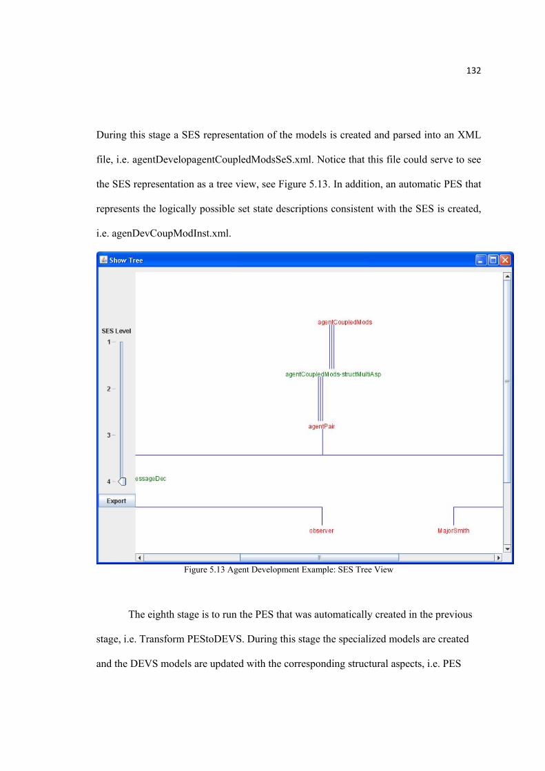
132
During this stage a SES representation of the models is created and parsed into an XML
file, i.e. agentDevelopagentCoupledModsSeS.xml. Notice that this file could serve to see
the SES representation as a tree view, see Figure 5.13. In addition, an automatic PES that
represents the logically possible set state descriptions consistent with the SES is created,
i.e. agenDevCoupModInst.xml.
Figure 5.13 Agent Development Example: SES Tree View
The eighth stage is to run the PES that was automatically created in the previous
stage, i.e. Transform PEStoDEVS. During this stage the specialized models are created
and the DEVS models are updated with the corresponding structural aspects, i.e. PES

133
transformed into DEVSJAVA models. This PES can also be modified by the developer to
create his own pruning and analyze the models of interest. The AutoDEVS tool allows
choosing the PES desired and then run it in the system, as shown in Figure 5.14.
Figure 5.14 Agent Development Example: Choosing a PES

134
The ninth stage is to create a set of test models to validate the system under
development, see Figure 5.15.
Figure 5.15 Agent Development Example: Generate Test Models
As seen in Figure 5.15, AutoDEVS lets the developer to choose the test models to create
from a list given. As described previously, these test models are based on minimal
testable I/O pairs restricted to messages and are created with the objective to verify the
correctness of the DEVS models. This feature is being developed and shall be available
in the near future.

135
The tenth stage is to verify the models created in the FDDEVS Models and SES
Builder DEVSJAVA SimView applications, i.e. Figure 5.16. Then modify the models
accordingly to the desired needs and start simulation.
Figure 5.16 Agent Development Example: Verifying models in SES, FDDEVS, and SimView

136
Figure 5.17 Agent Development Example: Running models in SimView
AutoDEVS process is iterative allowing return to modify the reference master
DEVS-model and the requirement’s specifications. Model continuity minimizes the
artifacts that have to be modified as the process proceeds. The design methodology
provides a process to transform the requirement’s specifications to a DEVS
representation supporting evaluation and recommendations for a feasible design.

137
Figure 5.18 AutoDEVS Life Cycle Process
As seen in Figure 5.18, AutoDEVS life cycle process combines system theory,
M&S framework, and model-continuity concepts. As illustrated, the tool bifurcates the
process into two main streams – system development and test suite development – that
converge in the system testing phase. The system development includes the definition of
requirements, capture of specifications to map formalized DEVS model components and
create a reference master model, and use of model continuity to execute model in the
DEVS real-time execution protocol, i.e. SimView. The test suite development includes
development of test models, and execution of test models against the system under test to
provide a feasible design from simulation and analysis results [Mit07].

138
CHAPTER 6. AUTODEVS TO AUTONOMOUS ROAD SURVEY SYSTEM DEVELOPMENT
6.1 Autonomous Road Survey System
The lack of constant road supervision within a mine increases the costs spent on
unexpected events, during operation. Examples of unexpected events include detection of
new paths or obstacles on roads. Such events, force the mine operation to stop executing
and either replan a route, or stop executing a specific task all together, thus halting
production and significantly affecting productivity. Improving the mine road supervision
to minimize costs caused by down-time of operation and optimizing the overall
performance is of significant importance to a mine operation. In terms of project
elaboration, the lack of designing structured information hierarchically and efficiently
could result in a complex, overwhelming project that complicates the analysis of the
system. Also, the development of intelligent systems involves the tedious task of
conducting intensive experimentation. To locate flaws in the behavior of multi-agent
system communication, simulation is proved to be a helpful and affordable tool in the
process of evaluating intelligent systems. On the other hand, it has been observed that
computers continue to become faster and increase in memory but they are still not enough
advanced to make sufficiently realistic models.
Autonomous Road Survey (ARS) demonstrates the effective application of
AutoDEVS and DEVS/SOA tool-based modeling and distributed simulation
methodologies in analytic studies of autonomous road survey within a standard mine.
This chapter discusses how ARS exploits both AutoDEVS methodologies and

139
DEVS/SOA framework to automate the development process of a system using the
model continuity methodology presented in Chapter 5. In addition, this chapter shows
how the tool provides high performance distributed simulation allowing developers to
make more realistic models. It is also shown how ARS provides an autonomous solution
for detecting and surveying roads, reducing risks and costs of human interaction in a
mine. The system presented in this chapter assumes that the real environment follows the
standards of creating roads within the mine and that there are a finite number of roads.
Some of these standards relate to how wide a road is, how roads are separated by borders
and how the vehicle can move to different levels thru open roads within a loop in the
mine, see Figure 6.1.
Figure 6.1Gold Mine in Canada

140
The ARS System follows the centralized approach where each robot communicates with
a CentralSystem. The CentralSystem coordinates each of the robots and helps them detect
roads in the mine. Though this system only includes one robot at this time, it can be
modified to include more robots that will essentially function as a team. This “team” of
robots can optimize the work and significantly decrease the amount of time it takes to
detect roads.
6.2 ARS Process
This example consists of a set of coupled models named CentralSystem, Runners and
SurveyEF as shown in Figure 6.2 below.

141
Figure 6.2 AutonomousRoadSurvey Main Abstraction Components
The ARS system intends to show how with the coordination of CentralSystem and
Runners operations, roads can be detected in a mine. As mentioned before, Runners has
only one Runner or robot at this time. The development of this example demonstrates
how modeling and simulation methodologies, based on the DEVS formalism, can support
model continuity and handle the development complexity for distributed robotic systems,
in addition to automating the development process of a system.

142
In this example, a user interface application is provided to allow the user to create
a virtual environment of the mine map, see Figure 6.3.
Figure 6.3 ARS User Interface Map Generator
As seen in Figure 6.3, this interface allows the user to load, create and save the map
desired for study. When the map has been saved, a file with all relevant coordinates is
created, i.e. Figure 6.4.

143
Figure 6.4 ARS Persistence Storage File
Once the virtual environment has been defined, the ARS System can be started. One of
the very first tasks of the system is to read the persistence storage file, i.e.
CustomRoadMap.txt, to load it into the SurveyEF (Experimental Frame) model and start
sending virtual data (position, surface state and wireless status) to the Runner and the
CentralSystem. When the Runner and CentralSystem models are started, they start
receiving data from all its couple models. For instance, the Runner receives data from the
SurveyEF model to know about the position, the surface state and the wireless status
from the current location and its neighbor cells. In this example, a cell corresponds to a
determined piece of road within a mine, i.e. a road is composed of multiple cells. The
Runner, on the other hand, surveys the road and sends data to the CentralSystem model to
update the current runner’s position, surface data and wireless status of the current

144
Runner. In addition, the Runner might receive data from the CentralSystem when the
Runner requests information, i.e. Runner finds an endless loop. The Runner uses an
artificial intelligence algorithm to move to the next position, depending on the surface
data from the neighbors. See Appendix A for more details on this algorithm.
The CentralSystem stores all the information received from the Runner and
processes all necessary information to produce the best approximation for the map of
interest. In order to show the users the current results of the ARS System, a 2D cell grid
plot is provided to show the output/results produced by the system during run-time
execution, see Figure 6.5.
Figure 6.5 ARS 2D Cell Grid Plot

145
As mentioned earlier, the CentralSystem receives data from the SurveyEF to update its
wireless adapter virtual component while the CentralSytem sends commands to the
Runner when this last has reached an endless loop road, i.e. all neighbor cells have been
surveyed already but not all expected cells have been surveyed yet. See Appendix B for
the artificial intelligence used by the CentralSystem model.
The SurveyEF main objective is to provide a virtual environment for the system
being developed. In addition, it contains a transducer model that stores relevant
information related to total time of execution and throughput for the jobs done by the
Runner. This transducer (JobT_Transducer) also records the data processed by the
CentralSystem related to map coordinates.
Finally, the CentralSystem produces a report that contains data produced by the
JobT_Transducer model containing data related to the cells surveyed, total time of
execution and throughput for the Runner completion task or job, see Figure 6.6.

146
Figure 6.6 ARS Report Generated by CentralSystem
6.3 Developing ARS Models using AutoDEVS
AutoDEVS was used during the elaboration of the ARS to automate the overall
development of the system. All of the structural aspects of the ARS system were
automatically developed and a great majority of the behavioral aspects were produced by
the tool, see Figure 6.7 for some of the requirement specifications for the ARS system.

147
Figure 6.7 ARS Requirement Specifications
Figure 6.8 illustrates the ARS model after following the AutoDEVS methodology as
described in Chapter 5, i.e. requirement specifications to a distributed real-time running
system. As said before, it covers all the structural aspects and a great majority of the
behavioral aspects as seen in Figure 6.9 for some of the models created.

148

149
Figure 6.8 ARS Models Produced by AutoDEVS: Structural Aspects

150
Figure 6.9 ARS Models Produced by AutoDEVS: Behavioral Aspects
ARS PES was defined using the AutoDEVS tool turning into the system desired to
analyze, see Figure 6.10. In this PES the number of runners, the generators, transducers
and the cells space for the ARS experimental frame were specified.

151
Figure 6.10 ARS PES Produced by AutoDEVS
Figure 6.11 shows part of the SES produced by the AuroDEVS tool.

152
Figure 6.11 ARS SES Tree View produced by the AutoDEVS.
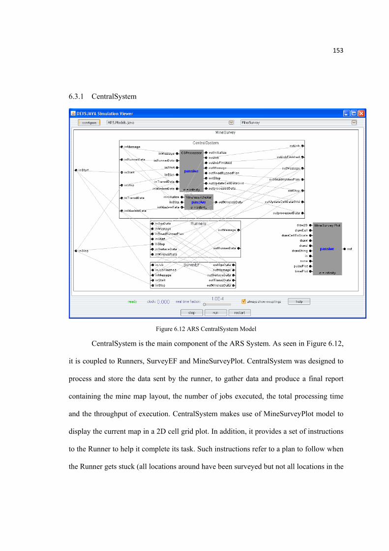
153
6.3.1 CentralSystem
Figure 6.12 ARS CentralSystem Model
CentralSystem is the main component of the ARS System. As seen in Figure 6.12,
it is coupled to Runners, SurveyEF and MineSurveyPlot. CentralSystem was designed to
process and store the data sent by the runner, to gather data and produce a final report
containing the mine map layout, the number of jobs executed, the total processing time
and the throughput of execution. CentralSystem makes use of MineSurveyPlot model to
display the current map in a 2D cell grid plot. In addition, it provides a set of instructions
to the Runner to help it complete its task. Such instructions refer to a plan to follow when
the Runner gets stuck (all locations around have been surveyed but not all locations in the

154
mine surface have been examined). See Appendix B for logic behind CentralSystem to
send the plan to the Runner.
Figure 6.13 CentralSystem State Diagram
Figure 6.13, shows the state’s flow of the CentralSystem. It initially starts in “passive”
state and as soon as it gets a “start” external message it changes to “active” state. From
the “active” state, the CentralSystem transitions to the “receive” state and simultaneously
outputs “initialize” to its components. At this point, the CentralSystem obtains data from
the Runner or sends a notification message specifying that it needs a plan in order to
continue moving. When receiving data from the Runner, the CentralSystem will
transition to state “processData”, where it will process the data received and update the
map being built at the CentralSystem. On the other hand, if receiving a message from the

155
Runner requesting a plan to continue, the CentralSystem will analyze the current data so
far obtained and come up with a new plan for the Runner or just finalize its execution.
When finalizing execution, the CentralSystem outputs a report with the total number of
jobs executed, map layout, the total processing time and the throughput of execution, i.e.
C:\AutonomousRoadSurvey. Note that every time the CentralSystem sends a new plan to
the Runner, a new job is could be created.
WirelessAdapter is coupled with the CentralSystem’s CSProcessor and is
responsible for sending the current wireless status of the wireless adapter to the
CentralSystem at a specified frequency. As seen in Figure 6.14, as soon as
WirelessAdapter gets a “start” external input” it goes to “active” state. From “active” it
receives WirelessData from the WirelessDataGenerator (SurveyEF) and sends this data to
the CSProcessor, remaining in the “active” state. Anytime the WirelessAdapter receives a
“stop” command it immediately passivates.

156
Figure 6.14 WirelessAdapter State Diagram
See Appendix C for the data structures used by the CentralSystem.
6.2.1 Runners

157
Figure 6.15 ARS Runners Model
Figure 6.15, represents the ARS Runners coupled model which contains
Runner_1. This Runner (Robot) is responsible for surveying the mine map and sending
all relevant information to the CentralSystem. This relevant information comes from the
Runner’s components, i.e. GpsReceiver which reads the current position of the Runner
and allows the Runner to learn about the points or locations already surveyed;
SurfaceSensor, which provides data read from the surface and helps the Runner detect
barriers within the road; and WirelessAdapter, which provides the status of the wireless
adapter to the Runner and this last to decide whether to send the information to the
CentralSytem or wait until there is better communication. Externally, the Runner receives
data from the generators located in the SurveyExperimentalFrame component, i.e. GPS

158
data, surface data and wireless adapter data. In addition, the Runner receives data from
CentralSystem to help the Runner determine where shall it should move or if a task has
been completed.
Figure 6.16 Runner State Diagram
Figure 6.16, illustrates the Runner state diagram. The Runner starts in “passive” state and
remains in this state until receiving a “start” command. As soon as the Runner receives
the “start” command, it initializes GpsReceiver, WirelessAdapter and SurfaceSensor.
After the Runner is done initializing, it passivates into “receive” state where it waits until
it has received the corresponding data from its components. From the “receive” state, the
Runner changes to the “sendData” state, where it process the data and outputs to the
CentralSystem. After sending the data, the Runner internally changes to the “receive”
state where the cycle continues until getting a “stop” external event and the Runner goes
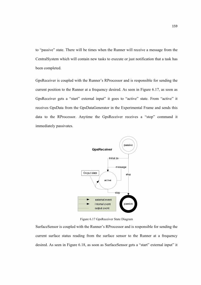
159
to “passive” state. There will be times when the Runner will receive a message from the
CentralSystem which will contain new tasks to execute or just notification that a task has
been completed.
GpsReceiver is coupled with the Runner’s RProcessor and is responsible for sending the
current position to the Runner at a frequency desired. As seen in Figure 6.17, as soon as
GpsReceiver gets a “start” external input” it goes to “active” state. From “active” it
receives GpsData from the GpsDataGenerator in the Experimental Frame and sends this
data to the RProcessor. Anytime the GpsReceiver receives a “stop” command it
immediately passivates.
Figure 6.17 GpsReceiver State Diagram
SurfaceSensor is coupled with the Runner’s RProcessor and is responsible for sending the
current surface status reading from the surface sensor to the Runner at a frequency
desired. As seen in Figure 6.18, as soon as SurfaceSensor gets a “start” external input” it

160
goes to “active” state. From “active” it receives surface sensor data from the
SurfaceDataGenerator (Experimental Frame) and sends this data to the Rprocessor,
remaining in the “active” state.
Anytime the SurfaceSensor receives a “stop” command it immediately passivates.
Figure 6.18 SurfaceSensor State Diagram
See Figure 6.14 for the WirelessAdapter State Diagram, Appendix C for the data
structures used by the Runner and Appendix A for the Runner’s Artificial Intelligence to
make decisions and move to the next point.
6.2.2 SurveyEF
Simulation methods are applied to test the correctness and efficiency of the ARS
system. In order to simulate and test the system, a simulation and testing environment is
developed, i.e. SurveyEF.

161
Figure 6.19 ARS SurveyEF Model
As seen in Figure 6.19, the SurveyEF Model is constituted of SEFCoordinator, MineMap,
Generators, Transducers and MineMap Plot. The SurveyEF provides the operational
formulation of the objectives that motivate the MineSurvey System.
The SEFCoordinator is the model responsible for coordinating and processing the
data coming from MineMap, Generators and Transducers and send it to CentralSystem
and Runners. SEFCoordinator puts together messages that contain the current position of

162
the Runner, the surface state at that location, the neighbor cells around the current
position and the wireless status at that point. It then sends these messages to the
CentralSystem’s WirelessAdapter and Runner’s GpsReceiver, SurfaceSensor and
WirelessAdapter. This model also sends data to the MineMapPlot when the custom road
map file is read during initialization, i.e. CustomRoadMap.txt.
Figure 6.20 SEFCoordinator State Diagram
Figure 6.20 represents a state diagram for the SEFCoordinator. As seen, the
model is started by an initialize command; it is in this time then that the SEFCoordinator
reads the file that contains data related to the environment or experimental frame of study.
After this model is initialized, it receives data from generators, transducers ,mineMap,
and message from other models such as CentralSystem and Runner. Notice that whenever
the model receives a stop command, the SEFCoordinator terminates execution.

163
The mineMap coupled model as seen in Figure 6.19 is composed of mapCoord
and Cells. The mapCoord coordinates the information coming from cells and
SEFCoordinator to create messages containing the current runner position and neighbor
cells. This model serves as a filter for the SEFCoodinator model since it parses the data
received from all cells and returns only the most relevant information to the
SEFCoordinator, i.e. current runner position and neighbor cells.
Figure 6.21 mapCoord State Diagram
Figure 6.21 shows the state diagram for the mapCoord model. This model is started by a
“start” external event; it then goes to the “active” state where it receives messages
coming from cells and SEFCoordinator, followed by parsing the data to then send
messages back to the SEFCoordinator. Anytime the model receives a “stop” commands,
it finishes execution.

164
GpsDataGenerator, SurfaceDataGenerator and WirelessDataGenerator were
developed to feed the GpsReceiver, SurfaceSensor and WirelessReceiver models used by
the Runner and the CentralSystem. These generators help test the correctness and
efficiency of the system and help detect flaws and improvements to the ARS. In addition,
these models were extended to include hardware interface abstract activity (gpsActivity,
surfaceActivity, wirelessActivity classes), which act as an abstract sensor/actuator
hardware interface to bridge between control models (CentralSystem and Runner) and the
environment model, i.e. mineMap. These abstract activity classes imitate the behavior
and interface functions of the hardware activity, so the control models can treat them in
simulation the same way as they treat the hardware activity in real execution. Similar to
the hardware activity, the abstract hardware activity regularly passes sensor data from the
mineMap environmental model, see Figure 6.22.

165
Figure 6.22 Abstract Activity Classes
Here is a code fragment for the GpsDataGenerator using the gpsActivity class:
public void deltint() { if (phaseIs("active")) { if (gpsActivity != null) { gpsActivity.kill(); } gpsActivity = new gpsActivity(AutonomousRoadSurvey.POLLING_INTERVAL); holdIn("active", AutonomousRoadSurvey.POLLING_INTERVAL, gpsActivity); }
...
public void deltext(double e, message x) { Continue(e); for (int i = 0; i < x.getLength(); i++) { if (this.messageOnPort(x, "outputFromActivity", i)) { ensembleBag messagesReceivedBag = x.valuesOnPort("outputFromActivity"); if(messagesReceivedBag.size() > 0) { gpsData = processMessages(messagesReceivedBag); }

166
}
As seen in the code fragment, the GpsDataGenerator is actually an atomic model. Its
internal transition function deltint starts or kills the gpsActivity which contains a thread
that returns GPS simulated data. Its external transition function deltext() handles the
receiver data sent from the environment model (gpsActivity class) and then passes this
receiver data to the SEFCoordinator which distributes the data to the GpsReceiver model
in the Runner coupled model.
Finally, a transducer is developed to calculate the total processing time and
throughput for the jobs executed by the Runner.
Figure 6.23 JobT_Transducer State Diagram
167
As seen in Figure 6.23, JobT_Transducer starts in the “passive” state until receiving a
“start” external input to then change the state to “active”. It remains in the “active” state
during the completion of the Transducer time. When the transducer time expires, it
outputs the number of jobs completed, the total processing time and the throughput of the
entire process. After finishing sending the data, the JobT_Transducer internally changes
to the “passive” state. Anytime it receives a “stop” message the JobT_Transducer is
changed to the final, “passive” state. In other words, the JobT_Transducer passivates. The
data sent by the transducer model is received by the CentralSystem and then stored in a
file, i.e. AutonomousRoadSurvey.txt.
6.4 Adding more Behavior Aspects to the ARS Models
Many of the behavioral aspects were developed using the AutoDEVS tool. However,
there was a need to modify these automated models to extend the functionality and
complete the ARS system. Such modifications include the following:
1) Add logic to mapCoord to request for start/end position and then request
neighbors (cellsData) from the start point.
2) Add logic to cells to respond to messages, i.e. request start/end/cellsData cells
from mapCoord.
3) Add logic to mapCoord to parse and filter data coming from cells and send it to
SEFCoordinator.
4) Add logic to SEFCoordinator sends corresponding data for the generators, i.e. use
data coming from the mapCoord.

168
5) Generators will parse data coming from SEFCoordinator and send it back.
6) SEFCoordinator will send the corresponding data coming from the generators out
to SurveyEF.
7) Add logic to GpsReceiver, SurfaceSensor and WirelessAdapter to parse data
coming from SurveyEF.
8) Add logic to RProcessor to parse data from components, i.e. GpsReceiver,
SurfaceSensor and WirelessAdapter.
9) Add logic to RProcessor to determine the next point to move depending on the
data received from its components.
10) Add logic in RProcessor to send runner data or request for roadRunnerPlan to
CentralSystem, i.e. messagesToSendQueue.
11) Add logic to RProcessor to process roadRunnerPlan.
12) Add logic to RProcessor to process Messages received from the CentralSystem,
i.e. processMessages.
13) Add logic to RProcessor to update MineMap as the Runner moves on.
14) Add logic to CSProcessor to process RoadRunner data.
15) Add logic to CSProcessor to process data from Transducers.
16) Add logic to CSProcessor to receive table dimensions and start and end point.
17) Add logic to CSProcessor to keep track of the cells already surveyed.
18) Add logic to CSProcessor to redirect runner when this last has found an endless
road.

169
19) Add logic to JobT_Transducer to calculate throughput and total processing time
for each job the runner needs to do.
20) Add logic to JobT_Transducer to send data to CSProcessor thru SEFCoord.
21) Add MACROS to ARS.
6.5 Stepwise Simulation, Deployment, and Execution
Different steps were applied to incrementally simulate and test the ARS system
before deploying the models to real hardware execution. These steps include central
simulation and distributed simulation.
6.5.1 Central Simulation
In central simulation, all the models, CentralSystem, Runner, SurveyEF
(including their abstract activities) reside in a single computer. DEVSJAVA SimView,
described in Chapter 5, allowed running and verifying the simulation of the ARS system.
Fast mode simulation was utilized first to simulate and test the Runner model. Based on
the simulation results, problems were traced and corrected. Two examples include, the
decisions made by the Runner to move to the next location depending on the current
position and its neighbor’s surface statuses, and path calculated by the CentralSystem and
followed by the Runner when the existence of an endless loop road within the mine has
been detected. After fast-mode simulation, real-time simulator is employed to run
simulation in a “timely” fashion. Within real-time simulation, a Graphic User Interface
(DEVSJAVA SimView) was used to show the model’s transactions, including the
exchange of messages, the transitions produced by internal/external events, and the

170
outputs produced by the models. In addition, adjusting the time scale for running the
models was very useful to speed up and quickly locate abnormal behaviors of the system.
The pseudo code to start fast-mode simulation and launch real-time simulation is
shown below.
//FAST-MODE SIMULATION /* Create a coordinator and pass RoadQualityMonitor (Diagraph model) */ coordinator coord = new coordinator(new AutonomousRoadSurvey()); /* Initialize coordinator */ coord.setTimeScale(0.0001); coord.initialize(); /* Produce external input */ coord.simInject(1, "inStart", new entity("start")); /* Provide the number of iterations to execute */ coord.simulate(1000000);
//REAL-TIME SIMULATION RTCoordinator rtCoord = new RTCoordinator(new AutonomousRoadSurvey()); rtCoord.initialize(); rtCoord.simInject(1, "inStart", new entity("start")); rtCoord.simulate(1000000);

171
6.5.2 Distributed Simulation
Figure 6.24 ARS Distributed Simulation
Figure 6.24 illustrates a DEVS simulation on SOA which is applied to a mine
space survey analysis which is the case that a client wants to see what the results are
coming out from the MineSurvey server to evaluate and take decisions. Deploying
workloads into multiple machines reduces the computational burden of servers as in the
case of a MineSurvey server, simulating the CentralSystem and ExperimentalFrame, and
Runner server, running the simulation for an independent runner. This approach allows
the users to make more realistic models and obtain simulation results quickly and
efficiently since the workloads are distributed among different servers.
DEVS/SOA was used to automate and make transparent distributed simulation for
the ARS system, as described in Chapter 4.

172
Figure 6.25 GUI snapshot of DEVSV/SOA client hosting distributed simulation
LocalHost simulation was first executed to ensure that the models were properly
modified to run in the DEVS/SOA environment. Some of these modifications include:
1) Make model to run as soon as it starts, i.e. no need of inject inputs.
2) Remove CellGridDataPlot logic.
3) Exclude having to read from an external file, i.e. hardcode roadmap.

173
4) Remove override statements.
5) Rename ViewableAtomic to atomic.
6) Rename ViewableDigraph to digraph.
7) Use strings for exchanging messaging between models.
8) Use getValOnPort and valuesOnPort to receive messages from ports.
9) Remove package line from each of the models.
10) Remove any code related to “simView” library.
11) Copy Java models to DEVSOA tool.
12) Follow the steps described in Chapter 4 for the DEVS/SOA tool.
Followed by the localhost simulation, distributed simulation was made, choosing one
server for the CentralSystem and SurveyEF, and another server for the Runner, see
Figure 6.27.
Figure 6.26 Assigning IP addresses to Models

174
Figure 6.27 DEVS/SOA: ARS Distributed Simulation
As seen in Figure 6.27, distributed simulation was made possible thanks to the
DEVS/SOA tool.
With a very limited change to the DEVS models, easy, transparent and fast
transition to distributed simulation was made. Despite the fact that this simulation took a
longer time to execute and finalize, it represented a more realistic simulation of the real
Autonomous Road Survey System.

175
6.5.3 Deployment and Execution
After passing these stepwise simulation-based tests, the final models are deployed
to the hardware execution environment. The basic task of the deployment stage is to
download models to their execution hardware. Runner models are downloaded to a real
robot and the CentralSystem models are downloaded to a wireless desktop, server or
laptop. For the Runner, real sensor/actuator interfaces are used. The SurveyEF,
environment model, is not needed anymore since the Runner now operates in the real
world. The final execution of the ARS system shall be relatively the same as that in the
simulation test.
6.5.4 Results and Discussions
Figure 6.28 MineMap of study (left) and AutonomousRoadSurvey output (right).

176
Figure 6.28 shows the first experiment executed, a simple square representing the
mine map layout. As seen, there is an open area inside the map, which represents the start
and the end of the map, the black cells represent the borders within the mine and the
white cells represent mine road cells. On the other hand, on the right figure the black cells
represent the border cells and the gray cells represent the cells that the Runner surveyed.
As illustrated, the expected results were successfully obtained.
Figure 6.29 MineMap II of study (left) and AutonomousRoadSurvey output (right).
Figure 6.29 shows the second experiment executed, two squares together with an
intersection representing the mine map layout of study. As seen, there is a green cell (top)
and a red cell (bottom) in the map, which represents the start and the end of the map
respectively, the black cells represent the borders within the mine and the white cells
represent mine road cells. On the other hand, on the right figure the black cells represent

177
the border cells and the gray cells represent the cells that the Runner surveyed. As
illustrated, the expected results were successfully obtained.
Figure 6.30 MineMap III of study (left) and AutonomousRoadSurvey output (right).
Figure 6.30 shows the third experiment executed, loading areas with intersections
representing the mine map layout of study. As seen, there is a green cell and a red cell in
the map, which represents the start and the end of the map respectively. The black cells
represent the borders within the mine and the white cells represent mine road cells. On
the other hand, in the right figure, the black cells represent the border cells and the gray
cells represent the cells that the Runner surveyed. As illustrated, the expected results
were successfully obtained.
As mentioned before, the simulation-based test methods can not only test the
correctness of control models, but also evaluate and analyze the performance of the
system to be developed. For example, the execution of the Runner while surveying the

178
mine map was totally dependent on the sensors/actuators. The more accurate data from
the sensors, the better performance and execution the Runner would have, i.e. GPS data
from receiver.
AutoDEVS was a key tool to develop the ARS system more effectively and in a
reduced amount of time as it allowed the development automation of the models used by
the ARS system. DEVS/SOA also played an important role for the development of
distributed simulation of the ARS system as it facilitated the development with small
modification to make this available.
These tools saved a huge amount of overhead by reducing the learning curve
needed when having to learn about models using DEVS methodologies. Similarly, the
time spent developing the ARS system was also significantly reduced and most of this
time was used on key behavioral aspects of the system such as the algorithm to follow
when surveying roads, i.e Runner moveNext.

179
CHAPTER 7. CONCLUSIONS AND FUTURE WORK
7.1 Conclusions
The need to improve productivity, quality and complexity hiding during systems
development has always been an important mission to be concerned for the success of an
organization. There exist many challenges that organizations face when willing to be
more successful than their competitors. Such challenges refer to the constant pressure to
deliver systems within minimum time and reduced cost, the rapid generation of
prototypes to enhance testing and detect flaws on early stages, and the need to shrink
development cycles and growing design complexity without compromising quality.
Originally introduced as formalism for discrete event modeling and simulation, the
DEVS (Discrete Event System Specification) methodology has become an engine for
advances within the wider area of information technology.
In this work, a distributed simulation-based system for an autonomous robotic survey
has been developed to show how this new DEVS-based tool called “AutoDEVS”
automates the systems development and exploits “model continuity” to maintain
coherence through the development process. It is shown that the methodology used by the
AutoDEVS tool, overcomes the “incoherence problem” through the development process.
Specifically, the methodology allows starting from system’s requirements in a
methodological way then produce designed control models which are tested and analyzed
by simulation methods and then easily deployed to the distributed target system for
execution. This was achieved by separating a system’s sensor/actuators interfaces from

180
its control model, which is the main design and test interest. During the process, virtual
sensor/actuators were developed for simulation-based test and ready for replacement by
real sensors/actuators during real system execution. By restricting virtual
sensors/actuators to sharing the same interface functions with their corresponding real
sensors/actuators to sharing the same interface functions with their corresponding real
sensors/actuators, the continuity of the control models was supported from simulation-
based design to real system execution.
SDLC Alternatives to SDLC AutoDEVS
Pros
1.Process and complete phases one at a time. 2.Test plans developed early on during life cycle. 3.Generates working software quickly and early. 4.High amount of risk analysis. 5.Customer interaction throughout development. 6.Teams have design freedom.
1.Allows the participation of end users. 2.Reduces the ambiguity produced in the elaboration phase. 3. Brings domain expert ideas together. 4.Prototypes allow emulating and building working systems. 5.Ability to rapidly change system design.
1.Flexible: changes in requirements do not impact the system. 2.Automates the development of models. 3.Allows developers to focus on the most critical parts of the system. 4.Alternative models can be selected, generated and evaluated. 5.Goes from requirements to a running real-time system. 6.Allows the creation of structured information hierarchically and efficiently. 7.Generates system test models. 8.Reduces the "incoherence problem" by introducing model continuity during the life cycle process. 9.Working software is provided on early stages. 10. Follows the Modeling, Simulation and Execution approach.

181
Cons
1.All requirements need to be explicitly defined. 2.No early prototypes are produced. 3.Each phase is rigid. 4.Project's success is highly dependent on risk analysis. 5.Relies heavily on the expertise of members. 6.Money and creative freedom can do a lot to boost the team productivity.
1.Big groups could become expensive and cumbersome. 2.Non-prepared sessions could waste professionals time. 3.Can lead to a succession of prototypes that never culminate in a satisfactory production application. 4.Potential for inconsistent designs. 5.Difficulty model reuse.
1. Limited to FD-DEVS domain. (However, this provides a skeleton for further elaboration into full DEVS.) 2. Requires understanding FD-DEVS and SES formalisms. To complete the design often requires in-depth understanding of full DEVS and the underlying system’s theory.
Table 7-1 AutoDEVS vs Other Methodologies.
As seen in Table 7-1, The AutoDEVS methodology employs simulation-based
methods to test the software under development. Specifically, to improve the traditional
software testing process where real-time embedded software needs to be hooked up with
real sensor/actuators and placed in a physical environment for system-level test and
analysis, a virtual testing environment was developed and allowed the software to be
effectively simulated and tested in a virtual environment, using virtual sensor/actuators.
Within this environment, a stepwise simulation-based test process was used so that
different aspects of a real-time software system could be tested and analyzed
incrementally.
It is demonstrated that the AutoDEVS methodology provides a natural and effective
way to model distributed real-time systems’ structure, behavior and timeliness. DEVS
Activity was employed to develop and allow models to interact with the external
environment. Within the AutoDEVS modeling, simulation and real-time execution

182
framework, models were and can be developed, simulated/tested by simulation methods,
and then executed in a distributed environment.
AutoDEVS together with DEVS formalism, FDDEVS, DEVSJAVA and DEVS/SOA
provided a robust and generic environment to build the AutonomousRoadSurvey discrete
event models, simulate and analyze the behavior of these models. In addition, AutoDEVS
and DEVSJAVA SimView allowed perceiving the flow of communications between
models and visually see its internal/external transitions and predict results before merging
the system to the real world. DEVS/SOA made the remote model execution and
distributed simulation available within a SOA framework, facilitating the deployment of
workloads into multiple servers, to increase the overall performance of the system and
make realistic models. The use of AutoDEVS methodology raised the importance of
simulation during the construction phase since it shows its usefulness using simulation to
detect and correct errors within the models, without having to wait until implementing the
system in a real hardware, increasing productivity in the system under development.
Furthermore, using the AutoDEVS tool permits to save lots of time and allow moving
further up faster on the core development.
From the ARS system behavior perspective, it can be seen that the faster the Runner
receives information from the sensors and adapters, the faster it will take decisions and
move to the next position. By using the ARS system, the costs spent in mines to survey
the road will be reduced and the human risk will be lowered. The ARS system provides a
solution and area of interest to automate the surveying done within a mine to increase
183
productivity and human risk. Using distributed simulation, the model could be developed
to reflect a more realistic system and validate every aspect of the system. In addition, this
system provides extensibility for different algorithms for the Runner and CentralSystem
to detect roads and scalability to simulate more Runners within the system. The
AutoDEVS methodology facilitated the design of structured information hierarchically
and efficiently for the AutonomousRoadSurvey system, allowing model reusability, i.e.
wirelessAdapter.
7.2 Future Work
The present research work has the following scope for future development:
• Towards DEVSJAVA framework
The DEVSJAVA and Simulation framework currently consumes a significant
amount of memory in the system being run. Improvements to enhance the
performance for large-scale cellular models can made, i.e. reduce cycle routine for
DEVSJAVA simulator. On the other hand, a toolbox similar to UML could be
provided to facilitate the developer to modify the models quicker, i.e. create
atomic model, coupled model, couplings, and define states and transitions. The
DEVSJAVA SimView simulation application could be improved to allow
backward simulation and detecting flaws more easily without having to restart the
entire simulation.
• Towards AutoDEVS framework

184
The AutoDEVS framework could be extended to automate the integration with
FD-DEVS and SESBuilder applications, i.e. automatic update to models when
these are modified in the other applications can be provided. Integration with the
DEVS/SOA environment could be extended on the AutoDEVS tool to automate
the conversion between DEVSJAVA and DEVS/SOA models. Extensions to the
tool to increase the automation of behavioral aspects to atomic models could be
made. An interface to easily execute stepwise simulation could be provided, i.e.
centralized simulation, decentralized simulation. distributed simulation, fast-mode
simulation, and real-time simulation. Allow AutoDEVS to accept new
spreadsheet requirements without compromising current models created.
• Towards the SESBuilder framework
Provide a toolbox to facilitate the creation of the SES tree directly and then follow
the top-down approach to create DEVSJAVA models automatically.
• Towards the ARS System
Future improvements to the ARS model can be made to the algorithms used for
the Runner and CentralSystem to survey the mine road. This system can be
extended to provide custom information when the runner is surveying the map,
for example where the “blind areas” (network communication) are within the
mine, what the quality of the surface road is while surveying, different types of
materials found around the area. In addition, it can be extended to allow the
system to function periodically to keep the CentralSystem and operators updated
with the latest information about the mine. Furthermore, this system could be

185
extended to make use of different number of Runners to survey and execute
operations in more effective and reduced time.
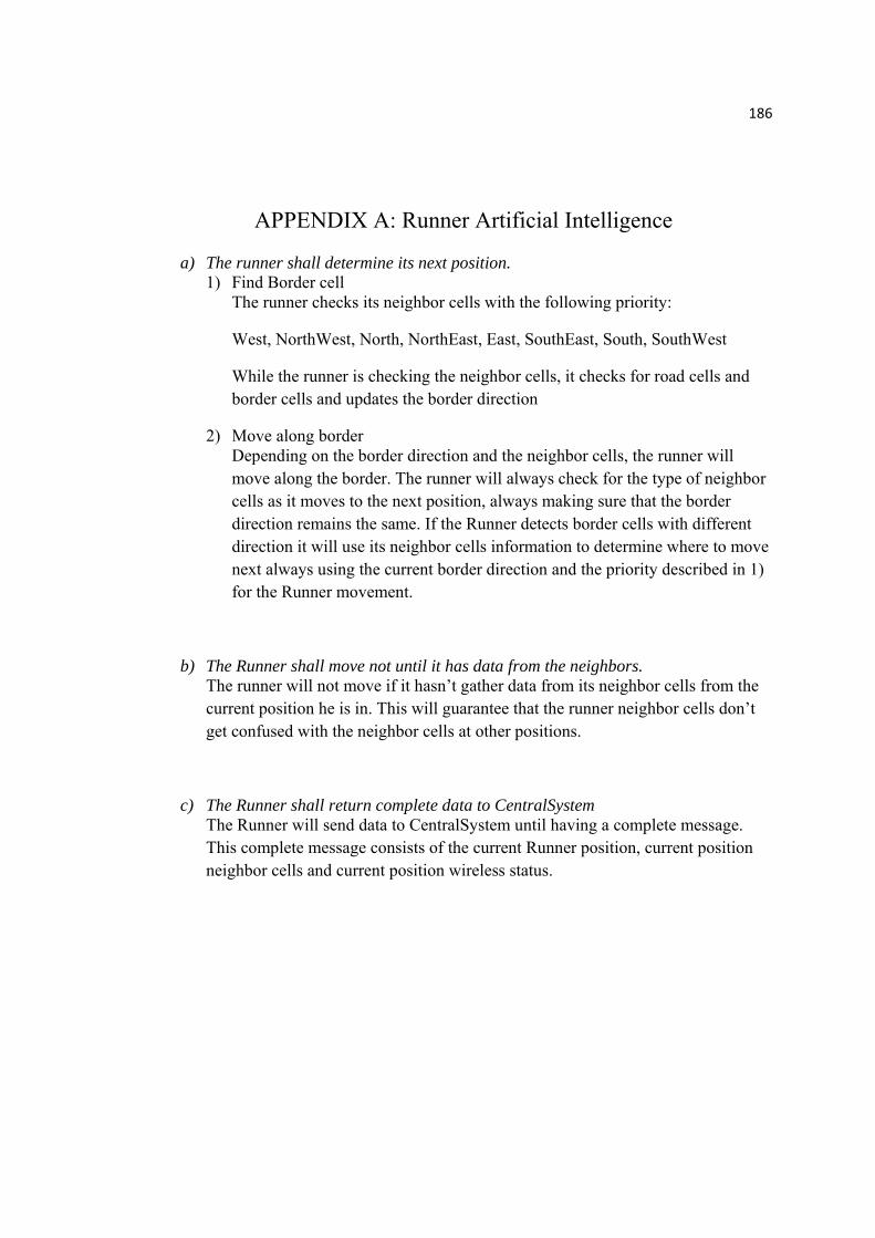
186
APPENDIX A: Runner Artificial Intelligence
a) The runner shall determine its next position. 1) Find Border cell
The runner checks its neighbor cells with the following priority:
West, NorthWest, North, NorthEast, East, SouthEast, South, SouthWest
While the runner is checking the neighbor cells, it checks for road cells and border cells and updates the border direction
2) Move along border Depending on the border direction and the neighbor cells, the runner will move along the border. The runner will always check for the type of neighbor cells as it moves to the next position, always making sure that the border direction remains the same. If the Runner detects border cells with different direction it will use its neighbor cells information to determine where to move next always using the current border direction and the priority described in 1) for the Runner movement.
b) The Runner shall move not until it has data from the neighbors. The runner will not move if it hasn’t gather data from its neighbor cells from the current position he is in. This will guarantee that the runner neighbor cells don’t get confused with the neighbor cells at other positions.
c) The Runner shall return complete data to CentralSystem The Runner will send data to CentralSystem until having a complete message. This complete message consists of the current Runner position, current position neighbor cells and current position wireless status.

187
APPENDIX B: CentralSystem Artificial Intelligence
a) Every Cell in the Mine Map must be surveyed before ending execution.
The way ARS makes sure every cell in the Mine Map is surveyed is by keeping track of the cells the Runner has surveyed in a table and the neighbor cells around the Runner position in a different table, i.e. if the Runner current position is 26, 8 then the tables will be filled as follows:
SurveyedCellsTable ExpectedCellsToSurveyTable Direction
26,8 26,7 west
25,7 northWest
25,8 north
25,9 northEast
26,9 east
27,9 southEast
27,8 south
27,7 southWest
Everytime the CentralSystem receives the position of the Runner, it updates the tables mentioned before. This will allow the CentralSystem to send the Runner to the corresponding pending cell that hasn’t been surveyed yet. This will happen everytime the Runner reaches an “endless point” position where all neighbor cells have been already surveyed until no cells are contained in the “ExpectedCellsToSurveyTable”.
b) CentralSystem shall send a plan to the Runner, to arrive to the nearest cell.
The way the CentralSystem creates the plan for the Runner when it has reached an “endeless point” is

188
1) Get the nearest cell from the ExpectedCellsToSurveyTable: return the cell that has the last minimum x coordenate absolute difference, i.e.
Runner Position
Cell
Expected Cells Table
abs(fromPoint- ExpectedPoint)
30,28 30,31 0,3
30,32 0,4
29,33 1,5
29,32 1,4
Therefore the nearest cell will be 30,32 because is the latest cell with minimum x coordenate difference.
2) Find shortest path from current Runner position to nearest cell: Find a border cell from the neigbors and move along the border, always checking if there are new cells in the way. If a new cell is detected, while going thru the nearest cell, then the shortest path algorithm will stop and return the path from the Runner position to the new cell detected in the way. Otherwise, it will use the SurveyCellsTable information to move along the border found.
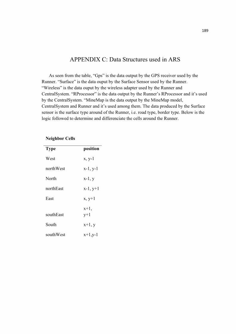
189
APPENDIX C: Data Structures used in ARS
As seen from the table, “Gps” is the data output by the GPS receiver used by the Runner. “Surface” is the data ouput by the Surface Sensor used by the Runner. “Wireless” is the data ouput by the wireless adapter used by the Runner and CentralSystem. “RProcessor” is the data output by the Runner’s RProcessor and it’s used by the CentralSystem. “MineMap is the data output by the MineMap model, CentralSystem and Runner and it’s used among them. The data produced by the Surface sensor is the surface type around of the Runner, i.e. road type, border type. Below is the logic followed to determine and differenciate the cells around the Runner.
Neighbor Cells
Type position
West x, y-1
northWest x-1, y-1
North x-1, y
northEast x-1, y+1
East x, y+1
southEast x+1, y+1
South x+1, y
southWest x+1,y-1

190
APPENDIX D: DEVS/SOA Installation
DEVS/SOA Environment (All the instructions MUST be followed) 1. Install Tomcat6.0: http://mirrors.isc.org/pub/apache/tomcat/tomcat-6/v6.0.14/bin/apache-tomcat-6.0.14.exe when jre dialog box appears during installation: Choose jre within jdk folder (C:\Program Files\Java\jdk1.6.0\jre) 2. Download Axis 2 binary distribution from http://ws.apache.org/axis2/download/1_3/download.cgi 3. Unzip Axis2 binary at C:/Axis2-1.3 4. Create environment variables: AXIS_HOME: C:/Axis2-1.3 JAVA_HOME: C:\Program Files\Java\jdk1.6.0 (Make sure it is jdk) CATALINA_HOME: C:\Program Files\Apache Software Foundation\Tomcat 6.0 5. Please perform the following replacements:
1. Replace the new Catalina.properties file at Tomcat6.0/conf 2. Replace the webapps folder at Tomcat 6.0/ (Unzip and replace) 3. Replace the temp folder at Tomcat6.0/ (Unzip and replace)
6. Run Tomcat6.0

191
REFERENCES
[Acc00] Accelerating Embedded e-development, Rational Rose Real Time, http://www.ghs.com/partners/rational/rose-rt.pdf
[Alb08] Jeannie Albrecht, Ryan Braud, Charles Killian, Priya Mahadevan, Kashi Vishwanath, and Amin Vahdat, An integrated software environment for distributed systems development, http://sysnet.cs.williams.edu/~jeannie/papers/plush-spie.pdf
[Ant00] G. Antoniol, B. Caprile, A. Potrich, P. Tonella, “Design-code traceability for object-oriented systems”. Annals of Software Engineering vol. 9: 35-58 (2000)
[Ant01] Magnus Antonson, Pernilla Hansson, Modeling of Real-Time Systems in UML with Rational Rose and Rose Real-Time based on RUP, http://www.google.com/url?sa=U&start=6&q=http://rise.uni.lu/tiki/se2c-bib_download.php%3Fid%3D455&usg=AFQjCNFqw153nT_4kw1OJ8hdmvqJ7D123w
[Ars08] Arsham Hossein, Systems Simulation, http://home.ubalt.edu/ntsbarsh/simulation/sim.htm#rnass
[Bag91] R. L. Bagrodia, C. Shen, “MIDAS: integrated design and simulation of distributed systems”, Software Engineering, IEEE Transactions on, Volume: 17, Issue: 10 , Oct. 1991
[Bap01] Bapat Vivek, Models of Packaging Efficiency, http://www.cadmen.com/sec_page/product_solve/Arena/Models.pdf 2001.
[Boy93] J. L. Boyd, Designing reactive systems for strong traceability, Carleton University, Ottawa, Ont., Canada, 1993
[Cas99] Castillo, O. Melin, P. , Modelling complex dynamical systems with a new fuzzy inferencesystem for differential equations: the case of robotic dynamic systems, South Korea, 1999, Volume 2.
[Cho01] Y. K. Cho, "RTDEVS/CORBA: A Distributed Object Computing Environment For Simulation-Based Design Of Real-Time Discrete Event Systems." Ph.D. thesis, University of Arizona, Tucson, AZ 2001

192
[Cho03] Y. K. Cho, X. Hu, and B. P. Zeigler: The RTDEVS/CORBA Environment for Simulation-Based Design Of Distributed Real-Time Systems, Simulation: Transactions of The Society for Modeling and Simulation International, 2003, Volume 79, Number 4
[Can97] Claudio A. Cañizares, Advantages and Disadvantages of Using Various Computer Tools in Electrical Engineering Courses, http://www.power.uwaterloo.ca/~claudio/papers/trace.pdf
[Cms08] CMS, Selecting a Development Approach,
http://www.cms.hhs.gov/SystemLifecycleFramework/Downloads/SelectingDevelopmentApproach.pdf
[EMF08] Eclipse Modeling Framework, http://www.eclipse.org/modeling/emf/
[Ger02] E. Gery, D. Harel, and E. Palachi, Rhapsody, "A Complete Life-Cycle Model-Based Development System", Integrated Formal Methods, Third International Conference, IFM 2002
[Gon02] F. G. Gonzalez, W. J. Davis, “A New Simulation Tool for the Modeling and Control of Distributed Systems”, SIMULATION: Transactions of the Society for Modeling and Simulation International, Volume 78, Number 9, 2002
[Gom01] M. Gomez., "Hardware-in-the-Loop Simulation", Embedded Systems Programming, December, 2001
[Ham95] Hammann, J.E.; Markovitch, N.A., Introduction to Arena [simulation software], http://ieeexplore.ieee.org/Xplore/login.jsp?url=/iel2/3475/10228/00478785.pdf?temp=x, 1995
[Hon97] J.S. Hong, and T.G. Kim, "Real-time Discrete Event System Specification Formalism for Seamless Real-time Software Development," Discrete Event Dynamic Systems: Theory and Applications, vol. 7, pp.355-375, 1997.
[HuX01] X. Hu, and B. P. Zeigler: An Integrated Modeling and Simulation Methodology for Intelligent Systems Design and Testing. Performance Metrics for Intelligent Systems Workshop, August, 2002.
[HuX02] X. Hu, and B. P. Zeigler: An Integrated Modeling and Simulation Methodology for Intelligent Systems Design and Testing. Performance Metrics for Intelligent Systems Workshop, August, 2002

193
[HuX04] Hu Xiaolin, A Simulation-based software development methodology for distributed real-time systems, http://acims.arizona.edu/PUBLICATIONS/PDF/Xiaolin_dissertation.pdf.
[Jan02] R. S. Janka, L. M. Wills, L. B. Baumstark, “Virtual Benchmarking and Model Continuity in Prototyping Embedded Multiprocessor Signal Processing Systems”, IEEE Transactions on Software Engineering, September 2002 (Vol. 28, No. 9)
[Jar08] Moath Jarrah, an automated methodology for negotiation behaviors in multi-agent engineering applications. Ph. D. Dissertation, Univ. of Arizona, 2008
[Kil07] C. Killian, J. W. Anderson, R. Braud, R. Jhala, A. Vahdat, Mace: language support for building distributed systems, Proc. Program. Lang. Design Implem., 2007. (accessed 21 Mar 2008) http://mace.ucsd.edu
[Lew08] http://codebetter.com/blogs/raymond.lewallen/archive/2005/07/13/129114.aspx
[Lou08] Technical Committee on Simulation, “Body of Knowledge on Simulation”, http://louisville.edu/speed/emacs/mrl/research/simulation/simulation/frame2.html
[Mar91] Martin, James, “Rapid Application Development”, Macmillan Publishing Co., Inc., 1991.
[Mat08] The MathWorks, http://www.mathworks.com/
[Mbd08] Model based design, http://en.wikipedia.org/wiki/Model_based_design
[Mit07] Saurabh Mittal, Devs unified process for integrated development and testing of service and testing fo service oriented architectures, Ph. D. Dissertation, Univ. of Arizona, 2007.
[Mit08] Saurabh Mittal, Bernard P. Zeigler, Moon Ho Hwang , XFD-DEVS, http://www.saurabh-mittal.com/fddevs/
[Öre05] Ören Tuncer, “Maturing Phase of the Modeling and Simulation Discipline”, Ottawa, Ontario, Canada, 2005, http://www.site.uottawa.ca/~oren/pubs-pres/2005/pub-0512-maturing.pdf
[Osi05] SOA Development,
http://www.osisoft.com/Resources/Newsletters/SOA+Development.htm, 2005.

194
[Pal06] Palaniappan, S., Sawheny, A., Sarjoughian, H.S., "Application of DEVS Framework in Construction Simulation", Winter Simulation Conference, Monterey, CA, http://acims.arizona.edu/PUBLICATIONS/PDF/constructionSim.pdf
[Plu08] Plush, http://plush.cs.williams.edu/index.html
[Pre97] R.S. Pressman, Software Engineering: A Practitioner's Approach, fourth ed. New York: McGraw-Hill, 1997.
[Pto08] The Ptolemy project, http://ptolemy.eecs.berkeley.edu/
[Ram01] B. Ramesh, M. Jarke, “Toward reference models for requirements traceability”, Software Engineering, IEEE Transactions on , Volume: 27, Issue: 1 , Jan. 2001
[Ran02] Randall S. Janka, Linda M. Wills, Lewis B. Baumstark, Jr., Virtual Benchmarking and Model Continuity in Prototyping Embedded Multiprocessor Signal Processing Systems, IEEE Transactions on Software Engineering, September 2002 (Vol. 28, No. 9)
[Ras01] Rastofer, U.; Bellosa, F., Component-based software engineering for distributed embedded real-time systems, Software, IEE Proceedings, Volume: 148 Issue: 3, June 2001
[Rob00] Paul Robertson, Robert Laddaga, and Howie Shrobe, "Introduction: the first international workshop on self-adaptive software", Lecture Notes in Computer Science, 2000, pp. 1-10
[Rts08] SESBuilder, http://www.rtsync.com/services/SESBuilder.html
[Sae08] Saehoon Cheon, Doohwan Kim, Bernard P Zeigler, System Entity Structure For XML Meta Data Modeling; Application to the US Climate Normals, IEEE International Conference on Information Reuse and Integration, Las Vegas, NV, July 2008.
[Sar01] Hessam S. Sarjoughian, Francois E. Cellier, Discrete Event Modeling and Simulation Technologies: A Tapestry of Systems and AI-Based Theories and Methodologies, p.31, Springer 2001.
[Ses08] http://www.sesbuilder.com/
[Sho98] Shokri, E.; Crane, P.; Kim, K., An implementation model for time-triggered message-triggered objectsupport mechanisms in CORBA-compliant COTS

195
platforms, http://ieeexplore.ieee.org/Xplore/login.jsp?url=/iel4/5419/14648/00666764.pdf?temp=x, 1998
[Sch00] W. Schulte, "Why Doesn't Anyone Use Formal Methods?", Integrated Formal Methods, Second International Conference, IFM 2000
[Sch02] Schulz, S.; Buchenrieder, K.J.; Rozenblit, J.W.: Multilevel testing for design verification of embedded systems. IEEE Design & Test of Computers Volume: 19 Issue: 2 , March-April 2002
[Sla01] Slan C. Shaw: Real-time Systems and Software, 2001, John Wiley & Sons
[Soa08] Service-oriented architecture, http://en.wikipedia.org/wiki/Service-oriented_architecture
[Son01] Feijun Song; Folleco, A.; An, E.: High fidelity hardware-in-the-loop simulation development for an autonomous underwater vehicle. OCEANS, 2001. MTS/IEEE Conference and Exhibition, Volume: 1 , 2001
[Ste02] Stephens Matt, Automated Code Generation, http://www.softwarereality.com/programming/code_generation.jsp,2002
[Vah02] A. Vahdat, K. Yocum, K. Walsh, P. Mahadevan, D. Kostic, J. Chase, D. Becker, Scalability and accuracy in a large-scale network emulator, Proc. 5th USENIX OSDI Symp., 2002. (Accessed 21 Mar 2008) http://modelnet.ucsd.edu
[Wel01] Wells, R.B.; Fisher, J.; Ying Zhou; Johnson, B.K.; Kyte, M.: Hardware and software considerations for implementing hardware-in-the-loop traffic simulation. Industrial Electronics Society, 2001. IECON '01. The 27th Annual Conference of the IEEE , Volume: 3 , 2001
[Wel01] Wells, R.B.; Fisher, J.; Ying Zhou; Johnson, B.K.; Kyte, M.: Hardware and software considerations for implementing hardware-in-the-loop traffic simulation. Industrial Electronics Society, 2001. IECON '01. The 27th Annual Conference of the IEEE , Volume: 3 , 2001
[Wiki] Automatic Programming, http://en.wikipedia.org/wiki/Automatic_programming [Wel01] Wells, R.B.; Fisher, J.; Ying Zhou; Johnson, B.K.; Kyte, M.: Hardware and software considerations for implementing hardware-in-the-loop traffic simulation. Industrial Electronics Society, 2001. IECON '01. The 27th Annual Conference of the IEEE , Volume: 3 , 2001

196
[Woo95] Wood, Jane and Silver, Denise; Joint Application Development, John Wiley & Sons Inc, ISBN 0-47104-299-4
[Wri08] http://www.garywwright.com/sdlc.php
[Zei76] Zeigler, B.P., Theory of Modelling and Simulation, Wiley, N.Y., 1976
[Zei00] B.P. Zeigler, T.G.Kim and H. Praehofer, “Theory of Modeling and Simulation: Integrating Discrete Event and Continuous Complex Dynamic Systems,” second edition Academic Press, Boston, 2000.
[Zei03] Bernard P.Zeigler, DEVS Today: Recent Advances in Discrete Event-based Information Technology, MASCOTS' 03, Orlando, FL, October 2003.