Autoassociative Memory Retrieval and

Spontaneous Activity Bumps in Small-World

Networks of Integrate-and-Fire Neurons

Anastasia Anishchenko

Department of Physics and Brain Science Program

Brown University, Providence RI 02912, USA

Elie Bienenstock

Division of Applied Mathematics,

Department of Neuroscience, Brain Science Program

Brown University, Providence RI 02912, USA

Alessandro Treves

Cognitive Neuroscience

SISSA - International School for Advanced Studies

Via Beirut 4, 34014 Trieste, Italy

March 3, 2004

1

Abstract

The metric structure of synaptic connections is obviously an important

factor in shaping the properties of neural networks, in particular the ca-

pacity to retrieve memories, with which are endowed autoassociative nets

operating via attractor dynamics. Qualitatively, some real networks in the

brain could be characterized as ’small worlds’, in the sense that the structure

of their connections is intermediate between the extremes of an orderly ge-

ometric arrangement and of a geometry-independent random mesh. Small

worlds can be defined more precisely in terms of their mean path length

and clustering coefficient; but is such a precise description useful to better

understand how the type of connectivity affects memory retrieval?

We have simulated an autoassociative memory network of integrate-

and-fire units, positioned on a ring, with the network connectivity varied

parametrically between ordered and random. We find that the network

retrieves when the connectivity is close to random, and displays the char-

acteristic behavior of ordered nets (localized ’bumps’ of activity) when the

connectivity is close to ordered. These two behaviors tend however to be

mutually exclusive, and the transition between the two occurs for values of

the connectivity parameter which are not simply related to the notion of

small worlds.

2

1 Introduction

Autoassociative memory retrieval is often studied using neural network models,

in which connectivity does not follow any geometrical pattern, – i.e. it is either

all-to-all or, if sparse, randomly assigned. Such networks can be characterized by

their storage capacity, expressed as the maximum number of patterns that can

be retrieved, which turns out to be proportional to the number k of connections

per unit. Networks with a regular geometrical rule informing their connectivity,

instead, can often display geometrically localized patterns of activity, i.e. stabilize

into activity profile ’bumps’ of width proportional to k. Recently, applications

in various fields have used the fact that small-world networks, characterized by

a connectivity intermediate between regular and random, have different graph

theoretic properties than either regular or random networks. In particular, small-

worlds have both a high clustering coefficient C and a short characteristic path

length L at the same time [1].

Here we consider a family of 1D networks of integrate-and-fire units, where

changing the parameter of randomness q allows to go from a regular network

(q = 0) in which all connections are relatively short-range, to a spatially random

network (q = 1) in which all connections can be considered to be long-range.

Intermediate values of q correspond to a biologically plausible combination of

long- and short-range connections. For q = 0 such a network spontaneously forms

3

activity bumps [16], and this property is expected to be preserved at least for

small values of q. For q = 1 the network behaves as an ordinary autoassociative

net [15, 10], and likewise this is expected to hold also for q < 1, as it does with a

simpler binary-unit model [7].

Can activity bumps and retrieval coexist?

We first explore how both the ability to retrieve, and to form bumps, change

with the degree of randomness q in the connectivity. We can then address the

question of whether the two abilities can coexist, at least in an intermediate regime

between q ' 0 and q ' 1.

Is the transition between the different regimes related to small worlds?

Since the ability to form bumps depends on the mutual support among active

units through excitatory feedback loops, one can expect it to persist as long as the

clustering coefficient C remains large, even as q grows above 0. Conversely, since

pattern retrieval depends on the propagation of the retrieval signal to all units

in the network independently of their location, one can expect robust retrieval to

require that the mean path length from one unit to any other one is still short,

even if q is below 1. Thus, one can expect an intermediate small-world regime of

coexistence between bumps and retrieval.

Can they coexist in more realistic networks, with integrate-and-fire dynamics?

Bohland and Minai [6], and more recently McGraw and Menziger [8] and

Morelli et al [7] have considered somewhat related issues with model networks

4

of binary neurons. Since the essential questions relate however to the stability

of bump states and of retrieval states, and the stability properties of attractor

networks are strongly affected by their dynamics [15, 14], we believe that to discuss

results in connection to real brain networks one has to consider integrate-and-fire

units. This is what we report here, presenting the result of computer simulations.

2 Model

2.1 Integrate-and-Fire Model

We consider a family of 1D networks of N integrate-and-fire units [17], arranged

on a ring. In the integrate-and-fire model we adopt, the geometry of a neuron is

reduced to a point, and the time evolution of the membrane potential Vi of cell i,

i = 1..N during an interspike interval follows the equation

dVi(t)

dt= −Vi(t) − V res

τm

+Rm

τm

(Isyn(t) + I inh(t) + Ii(t)

)(1)

where τm is the time constant of the cell membrane, Rm its passive resistance, and

V res the resting potential. The total current entering cell i consists of a synaptic

current Isyni (t) due to the spiking of all other cells in the network that connect to

cell i, an inhibitory current I inh(t), which depends on the network activity, and a

small external current Ii(t), which represents all other inputs into cell i.

The last, external component of the current can be expressed through a di-

5

mensionless variable λi(t) as

Ii(t) = λi(t)(Vth − V res)/Rm (2)

We use a simplified model for the inhibition, where it depends on the excitatory

activity of the network. The inhibitory current is the same for all neurons at a

given moment of time, and changes in time according to the equation

dI inh(t)

dt= − 1

τinhI inh(t) + λinh (V th − V res)

NRmr(t) (3)

where λinh is a dimensionless inhibitory parameter of the model and r(t) is a rate

function characterizing the network activity up to time t:

r(t) =∑

i

∑

{ti}

∫ t

−∞K(t − t′)δ(t′ − ti)dt′ (4)

The kernel K(t − t′) we use for our simulations is a square wave function lasting

one time step ∆t of the integration, so that r(t) is just a total number of spikes

in the time interval ∆t.

As Vi reaches a threshold value V thr, the cell emits a spike, after which the

membrane potential is reset to its resting value V res and held there for the duration

of an absolute refractory period τref . During this time the cell cannot emit further

spikes no matter how strongly stimulated.

2.2 Synaptic Inputs

All synapses between neurons in the network are excitatory, and the synaptic

conductances are modeled as a difference of two exponents with time constants

6

τ1 and τ2, such that τ2 is of the order of τm and τ1 >> τ2. The synaptic current

entering cell i at time t then depends on the history of spiking of all cells that

have synapses on i:

Isyni (t) =

τm

Rm

∑

j 6=i

∑

{tj}

∆Vji

τ1 − τ2

(e−

t−tjτ1 − e

−t−tjτ2

)(5)

where {tj} are all the times before time t when neuron j produced a spike and

∆Vji is a size of the excitatory postsynaptic potential (EPSP) in neuron i evoked

by one presynaptic spike of neuron j.

The relative size of the evoked EPSP determines the efficacy of synapse ji:

∆Vji = λsyn (V th − V res)

Ncji[1 + Jji] (6)

where λsyn is the model parameter characterizing synaptic excitation, cji is 0 or 1

depending on the absence or presence of the connection from neuron j to neuron

i, and Jij is modification of synaptic strength due to Hebbian learning, which will

be described later (Section 2.4).

2.3 Connectivity

In our model, all connections in the network are uni-directional, so the connectivity

matrix is not symmetrical. We use a special procedure for creating connections,

after [1]: the probability of one neuron to make a connection to another depends

on a parameter q in such a way, that changing q from 0 to 1 allows one to go from

a regular to a spatially random network.

7

A regular network (q = 0) in this case is a network where connections are

formed based on a Gaussian distribution. The probability to make a connection

from neuron i to neuron j in such a metwork is

P0(cij) = e−|i−j|2

2σ2 (7)

where |i − j| is the minimal distance between neurons i and j on the ring. This

results in an average number of connections per neuron k ≈√

2πσ (actually,

k <√

2πσ because of the finite length of the ring).

In a random network (q = 1), the probability of creating a connection does

not depend on the distance between neurons:

P1(cij) = k/N (8)

Intermediate values of q thus correspond to a biologically plausible combination

of long- and short-range connections:

Pq(cij) = (1 − q)e−|i−j|2

2σ2 + qk

N(9)

The parameter q is referred to as the ‘randomness’ parameter, following Watts

and Strogatz, who used a similar procedure for interpolating between regular and

random graphs.

As originally analyzed by Watts and Strogatz[1], the average path length and

clustering coefficient in a graph wired in this way both decrease with q, but their

functional dependence takes different shapes. Thus, there is a range of q where

8

the clustering coefficient still remains almost as high as it is in a regular graph,

while the average path length already approaches values as low as for random

connectivity. Graphs that fall in this range are called small-world graphs, referring

to the fact that for the first time this type of connectivity was explored in a context

of social networks [4]. In this context the average (or characteristic) path length L

can be thought of as the average number of friends in the shortest chain connecting

two people, and the clustering coefficient C as the average fraction of one’s friends

who are also friends of each other.

In a neural network, L corresponds to the average number of synapses that

need to be passed in order to transmit a signal from one neuron to another, and

thus depends on the number and distribution of long-range connections. The

clustering coefficient C characterises the density of local connections, and can be

thought of as the probability of closing a trisynaptic loop (the probability that

neuron k is connected to i, given that some neuron j which receives from i connects

to k).

2.4 Hebbian plasticty

Associative memory in the brain can be thought of as mediated by the Hebbian

modifiable connections. Modifying connection strength corresponds to modifying

the synaptic efficacy of Eq. 6:

9

Jij =1

M

p∑

µ=1

(ηµ

i

〈η〉 − 1

)(ηµ

j

〈η〉 − 1

)(10)

where ηµi is the firing rate of neuron i in the µth memory pattern, 〈η〉 is the

average firing rate, the network stores p patterns with equal strength, and M is

a normalization factor. The normalization factor should be chosen to maximally

utilize the useful range of synaptic efficacy, which could be done by equalizing its

variance with its mean. In order to preserve the non-negativity of each efficacy,

in Eq. 6 we set Jij = −1 whenever (1 + Jij) < 0.

We draw patterns of sparseness a from a binary distribution, so that ηµi = 1/a

with probability a and ηµi = 0 with probability 1−a. The ’average firing rate’ 〈η〉

in this case is equal to 1.

2.5 Experimental Paradigm

After the connections have been assigned and the synaptic efficacies modified by

storing memory patterns, we randomize the starting membrane potentials for all

the neurons:

V sti = V res + β(V th − V res)ni (11)

where β = 0.1 is a constant and ni is a random number between 0 and 1, generated

separately for each neuron i. We then let the network run its dynamics.

After a time t0, a cue for one of the p patterns (for instance, pattern µ) is given,

in the form of an additional cue current injected into each cell. The cue current is

10

injected at a constant value up to the time t1, and then decreased linearly to 0 so

that it becomes 0 at time t2. Thus, for the dimensionless current in (2) we have

λi(t) = λ0 + λcuef(t)(ηµi − 1) (12)

where λ0 > 0 is a constant, dimensionless external current flowing into all cells,

λcue is a dimensionless cue current parameter, and

f(t) =

0 : t < t0 or t2 ≤ t

1 : t0 ≤ t < t1

1 − t−t1t−t2

: t1 ≤ t < t2

(13)

If the cue is partial – for example, the cue quality ρ = 25% – then a continuous

patch of the network, comprised of 25% of the length along the network ring,

receives the cue for pattern µ, whereas the rest of the network receives a random

pattern. (In the simulations, the random pattern on the rest of the network has a

higher average activity than the original patterns, which makes the overall network

activity rise slightly during application of the cue.)

During the time tsim of the simulation, spike counts (numbers of spikes fired

by each neuron), are collected in sequential time windows of length twin:

ri(t) =∑

{ti}

∫ t

t−twin

δ(t′ − ti)dt′ (14)

We then look at the geometrical shape of the network activity profile in each

window, and at the amount of overlap of this activity with each of the patterns

stored.

11

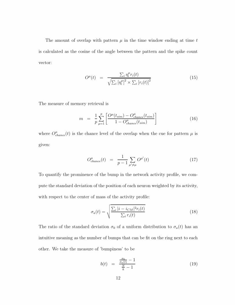
The amount of overlap with pattern µ in the time window ending at time t

is calculated as the cosine of the angle between the pattern and the spike count

vector:

Oµ(t) =

∑i η

µi ri(t)√∑

i [ηµi ]2 ×∑

i [ri(t)]2

(15)

The measure of memory retrieval is

m =1

p

p∑

µ=1

[Oµ(tsim) − Oµ

chance(tsim)

1 − Oµchance(tsim)

](16)

where Oµchance(t) is the chance level of the overlap when the cue for pattern µ is

given:

Oµchance(t) =

1

p − 1

∑

µ′ 6=µ

Oµ′(t) (17)

To quantify the prominence of the bump in the network activity profile, we com-

pute the standard deviation of the position of each neuron weighted by its activity,

with respect to the center of mass of the activity profile:

σa(t) =

√√√√∑

i |i − iCM |2ri(t)∑i ri(t)

(18)

The ratio of the standard deviation σ0 of a uniform distribution to σa(t) has an

intuitive meaning as the number of bumps that can be fit on the ring next to each

other. We take the measure of ’bumpiness’ to be

b(t) =

σ0

σa(t)− 1

Nk− 1

(19)

12

For an easier comparison with the memory retrieval measure, we compute the

’bumpiness’ of a particular network in the last time window of the simulation

(t = tsim), and then average over simulations with different cues.

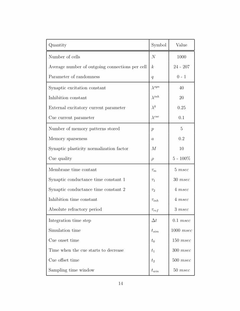
Table 1: Parameters Used for the Simulations.

13

Quantity Symbol Value

Number of cells N 1000

Average number of outgoing connections per cell k 24 - 207

Parameter of randomness q 0 - 1

Synaptic excitation constant λsyn 40

Inhibition constant λinh 20

External excitatory current parameter λ0 0.25

Cue current parameter λcue 0.1

Number of memory patterns stored p 5

Memory sparseness a 0.2

Synaptic plasticity normalization factor M 10

Cue quality ρ 5 - 100%

Membrane time contant τm 5 msec

Synaptic conductance time constant 1 τ1 30 msec

Synaptic conductance time constant 2 τ2 4 msec

Inhibition time constant τinh 4 msec

Absolute refractory period τref 3 msec

Integration time step ∆t 0.1 msec

Simulation time tsim 1000 msec

Cue onset time t0 150 msec

Time when the cue starts to decrease t1 300 msec

Cue offset time t2 500 msec

Sampling time window twin 50 msec

14

Note: Ranges are indicated for quantities that varied within runs.

3 Results

3.1 Graph-Theoretic Properties of the Network

Finding an analytical approximation for the characteristic path length L is not

a straightforward calculation. Estimating the clustering coefficient C for a given

network is, however, quite easy. In our case, integrating connection probabilities

(assuming, for the sake of simplicity, an infinite network) yields the analytical

estimate

C(q) =

[1√3− k

N

](1 − q)3 +

k

N(20)

or, after normalization,

C ′(q) =C(q) − Cmin

Cmax − Cmin= (1 − q)3 (21)

which does not depend either on the network size N , or on the number k of

connections per neuron.

Once connections have been assigned, both L and C can be calculated nu-

merically. Keeping the number of connections per neuron k > ln N ensures that

the graph is connected [3], i.e. that the number of synapses in the shortest path

between any two neurons does not diverge to infinity.

15

The results of numerical calculations are shown in Fig. 1A. The characteristic

path length and the clustering coefficient both decrease monotonically with q,

taking their maximal values in the regular network and minimal values in the

random network. Similar to what was described by Watts and Strogatz[1][2], L

and C decrease in different fashions, with L dropping down faster than C. For

example, for q = 0.1, C ′ is at 52% of its maximal value C ′(0) ≡ 1, while L−Lmin

has already dropped to 8% of L(0) − Lmin.

Comparing the clustering coefficient estimated analytically with the simplified

formula (20) and the one calculated numerically shows some minor discrepancy

(Fig. 1B), which is due to the fact that analytical calculations were performed for

an infinite network.

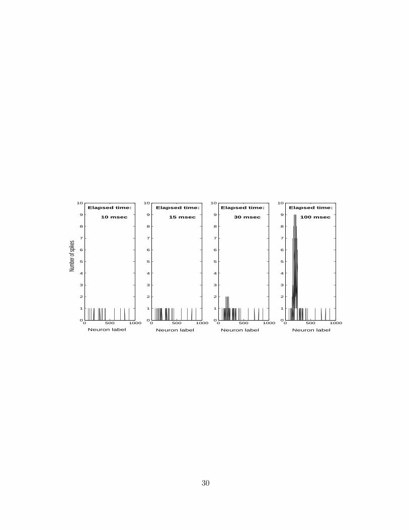
3.2 Bumps Formation in a Regular Network

Networks whose connectivity follows a strict geometrical order spontaneously form

bumps in their activity profile, as shown in Fig. 2. Bumps are formed before the

presentation of a pattern specific cue, and can either persist, or be temporarily

or permanently altered or diplaced after cue onset. Robust bumps, which remain

after the cue has been introduced and then removed, tend to form only for regular

or nearly regular connectivity (small values of q). Fig. 3A exemplifies this behavior

for a network with k = 41 connections per unit, and different values of q. In the

example, a robust single bump forms for q = 0 and q = 0.2. A double bump forms

16

for q = 0.4, and is relocated to a different section of the ring following the cue.

A very noisy triple bump is barely noticeable towards the end of the simulation

for q = 0.6, and no bumps can be really observed for random or nearly random

nets, q = 0.8 and q = 1. Thus bump formation appears to be strongly favored by

a regular connectivity, as expected.

3.3 Memory Retrieval in a Random Network

Fig. 3B shows the overlaps with the different memory patterns in the same simu-

lations used for Fig. 3A, with k = 41. The cue which is presented after 150msec

is correlated with the second pattern along one fourth of the ring, and it reliably

enhances the overlap with the second pattern during cue presentation, whatever

the value of q. By chance, the second (and to some extent the fifth) pattern tends

to have an elevated initial overlap also before the presentation of the cue, a be-

haviour often observed in autoassociative nets and due to fluctuations. Despite

this early ’advantage’, once the pattern specific cue has been completely removed

(after 500msec, that is after the first 10 frames in the Figure) the overlap with the

cued pattern returns to chance level, except in the case of a fully random (q = 1)

or nearly random (q = 0.8) connectivity. Thus the randomness in the connectivity

appears to favor memory retrieval, as expected, presumably by ensuring a more

rapid propagation of the retrieval signal to the whole network, along shorter mean

paths.

17

3.4 Bumps and Memory in Networks of Different Degrees

of Order

Fig. 4 summarizes the results of simulations like those of Fig. 3, for k = 41. The

spontaneous activity bumps, which are formed in the regular network, can be

observed, somewhat reduced, up to q = 0.4. For larger values of q the bumpiness

measure drops to a value close to zero. Storing random binary patterns on the

network does not affect the bumps, but the retrieval performance appears to be

very poor for small q. However, as the randomness increases (q ≥ 0.6), robust

retrieval can be observed even for partial cues. For these reference values of the

number of connections (k = 41) and cue quality (ρ = 25%) the transitions from

bumps to no bumps and from no retrieval to retrieval are both fairly sharp, and

both occur between q = 0.4 and q = 0.6.

Results are not always so clear cut, as shown in Fig. 5, which reports the

measures of retrieval averaged over the 5 cued patterns but for each of 3 network

realizations, and as a function of cue quality. It is apparent that there is consid-

erable variability in performance, which is reduced by taking a further average

over the 3 network realizations, as in Fig. 5D. In this panel, retrieval performance

appears to depend smoothly on q and ρ. For sufficiently large cues, ρ ≥ 25%

the network retrieves reasonably well when it is regular or nearly regular, q = 1

or q = 0.8, although the normalized overlap is far from its maximum at 1. The

18

overlap is reduced for q = 0.6, and drastically reduced, but not down to zero, for

more regular networks, q ≤ 0.4. For lower cue quality, ρ = 15%, 10%, all average

overlap values are reduced, and they are around zero for regular or nearly regular

nets. For even lower cue quality, ρ = 5%, no retrieval really occurs.

The non-zero overlap measures reached with large cues reflect what may be

called remnant magnetization in a spin system, and make the distinction between

retrieval and no retrieval somewhat fuzzier. Nevertheless, whatever the size of the

cue, it is apparent that there is a well defined transition between two behaviors,

bump formation and retrieval, which for k = 41 is concentrated between q = 0.4

and q = 0.6. The region of coexistence, if it exists, is in this case limited.

Changing k does not affect the qualitative network behavior, as shown in Fig. 6,

in that whatever k there is a transition between bump formation in nearly regular

networks (on the left in each panel) and retrieval in nearly random networks(on

the right). The transition is not always as sharp as in Fig. 4, in part because

there is no averaging over 3 different realizations, and in some cases one could

describe an individual network as able to both form bumps and retrieve memory

patterns to some extent. When the number of connections is very limited (k = 24),

both retrieval and bump formation are weak, when they at all occur. For more

extensive connections the degree of bumpiness, as quantified by our measure, stays

constant at a value close to 0.6 for regular networks. The range of the parameter

of randomness, over which bump formation occurs, shrinks with increasing k, and

19

in the case of k = 207 the bumpiness for q = 0.2 is already down to roughly 1/3

of its value for the regular network.

The retrieval measure, instead, reaches higher values the larger is k, reflecting

the larger storage capacity of networks with more connections per unit. In our

simulations the number of patterns is fixed at p = 5, but the beneficial effect of

a more extensive connectivity is reflected in higher values for the overlap with

the retrieved patterns. In parallel to bump formation, the range of q values over

which the network retrieves well appears to increase with k, so that for k = 207

essentially only regular networks fail to retrieve properly. Overall the transition

from no retrieval to retrieval appears to occur in the same q-region as the transition

from bumps to no bumps, and this q-region shifts leftward, to lower q values, for

increasing k, as is evident in Fig. 5.

This result contradicts the expectation that one or both of these transitions be

simply related to the small-world property of the connectivity graph. As shown

above, the normalized value of the clustering coefficient, whose decrease marks

the right flank of the small-world regime, is essentially independent of k, as it is

well approximated, in our model, by the simple function (1 − q)3. The transition

between a bump regime and a retrieval regime, instead, to the extent that it

can be defined, clearly depends on k, and does not, therefore, simply reflect a

small-world related property.

20

4 Discussion

Although small-world networks have been recently considered in a variety of stud-

ies, the relevance of a small-world type of connectivity for associative memory

networks has been touched upon only in a few papers. Bohland and Minai [6]

compare the retrieval performance of regular, small-world and random networks

of an otherwise classic Hopfield model with binary units. They conclude that

small-world networks with sufficiently large q approach the retrieval performance

of random networks, but at the cost of a reduced total wire length. Note that wire

length is measured taking the physical distance between connected nodes into ac-

count, while path length is just the number of nodes to be hopped on in order to

connect from one to another node of a pair. This result of reduced wire length for

similar performance is likely quite general, but it relies on the small-world prop-

erty of the connectivity graph only in the straightforward sense of using up less

wiring (which is true also for values of q above those of the small-world regime);

and not in the more non-trivial sense of using also the high clustering coefficient

of small-world networks. The second result obtained by Bohland and Minai is

that small-world nets can ’correct’ localized errors corresponding to incomplete

memory patters quicker than more regular networks (but slower than more ran-

dom network). This again illustrates behavior intermediate between the extremes

of a well performing associative memory network with random connections, and

21

of a poorly performing associative memory network with regular connections.

McGraw and Menziger [8] similarly compare the final overlap reached by asso-

ciative networks of different connectivity, when started from a full memory pattern

(this they take to be a measure of pattern stability) and from a very corrupted

version of a memory pattern (this being a measure of the size of a basin of attrac-

tion). In terms of both measures small worlds again perform intermediate between

regular and random nets, and in fact more similarly to random nets for values of

q ' 0.5, intermediate between 0 and 1. They go on to discuss the property of an-

other type of connectivity, the scale-free network, in which a subset of nodes, the

’hubs’, receive more connections than the average, and therefore unsurprisingly

performs better on measures of associative retrieval restricted to the behavior of

the hubs themselves.

In summary, neither of these studies indicates a genuine non-trivial advantage

of small-world connectivity for associative memories.

In our study, we considered integrate-and-fire units instead of binary units,

so as to make somewhat more direct contact with cortical networks. More cru-

cially, we also investigated, besides associative memory, another behavior, bump

formation, which can also be regarded as a sort of emergent network computa-

tion. Morelli et al in a recent paper [7] study an analogous phenomenon, i.e. the

emergence, in an associative memory with partially ordered connectivity, of dis-

crete domains, in each of which a different memory pattern is retrieved. Although

22

broadly consistent with our findings insofar as retrieval goes, the phenomenon

they study is almost an artefact of the binary units used in their network, while

we preferred to consider emergent behavior relevant to real networks in the brain.

We wondered whether connectivity in the small-world regime might be reflected

in an advantage not in performing associative retrieval alone, but in the coexis-

tence of retrieval and bump formation. We failed to observe this coexistence in

practice, as networks go, with increasing q, from a bump forming regime with no

(or very poor) retrieval - to a retrieving regime with no bumps. Further, we found

that the critical transition q values are not simply related to the boundaries of the

small-world region, in that they also depend, at least, on the average connectivity

k.

Because of its simulational character, our study cannot be taken to be exhaus-

tive. For example, the partial retrieval behavior occurring for small q might in fact

be useful when sufficiently few patterns are stored, p small. In our simulations,

p = 5, but then the whole network was limited in size and connectivity. More-

over, a 2D network, which models cortical connectivity better than our 1D ring,

might behave differently. Further, memory patterns defined over only parts of the

network, which again brings one closer to cortical systems, might lead to entirely

different conclusions about the coexistence of bump formation and associative re-

trieval. These issues are left for further work, and in part they are addressed in

an analytical study of networks of threshold-linear units by Roudi and Treves (in

23

preparation).

Acknowledgments

We are grateful to Francesco P. Battaglia and Haim Sompolinsky for their help

at the early stage of the project; to the EU Advanced course in Computational

Neuroscience (Obidos, 2002) for the inspiration and opportunity to develop the

project; and to the Burroughs Wellcome Fund for partial financial support.

24

References

[1] D. J. Watts, S. H. Strogatz, Collective dynamics of ’small-world’ networks,

Nature 393 (1998) 440-442

[2] D. J. Watts, The dynamics of networks between order and randomness,

Princeton University Press, Princeton NJ (1999)

[3] B. Bollobas, Random Graphs, Academic Press, New York (1985)

[4] S. Milgram, The small-world problem, Psychol. Today 2 (1967) 60-67

[5] E. Bienenstock, On the dimensionality of cortical graphs, J Physiology-Paris

90 (3-4) (1996) 251-25

[6] J. W. Bohland, A. A. Minai, Efficient associative memory using small-world

architecture, Neurocompution 38-40 (2001) 489-496

[7] L. G. Morelli, G. Abramson, M. N. Cuperman, Associative memory on a

small world neural network, arXiv:nlin.AO/0310033 v1 (2003)

[8] P. N. McGraw, M. Menzinger, Topology and computational performance of

attractor neural networks, arXiv:cond-mat/0304021 (2003)

[9] J. J. Hopfield, Neural networks and physical systems with emergent collective

computational abilities, Proc Natl Acad Sci USA 79 (1982) 2554-2558

25

[10] B. Derrida, E. Gardner, A. Zippelius, An exactly soluble asymmetric neural

network model, Europhysics Letters 4 (1987) 167-174

[11] M. V. Tsodyks, M. V.Feigel’man, The enhanced storage capacity in neural

networks with low activity level, Europhysics Letters 6 (1988) 101-105

[12] F. P. Battaglia, A. Treves, Attractor neural networks storing multiple space

representations: A model for hippocampal place fields, Physical Review E 58

(1998a) 7738-7753

[13] F. P. Battaglia, A. Treves, Stable and rapid recurrent processing in realistic

autoassociative memories, Neural Computation 10 (1998b) 431-450

[14] A. Treves, Mean-field analysis of neuronal spike dynamics, Network 4 (1993)

259-284

[15] D. J. Amit, N. Brunel, Dynamics of a recurrent network of spiking neurons

before and following learning, Network 8 (1997) 373-404

[16] R. Ben-Yishai, R. Lev Bar-Or, H. Sompolinsky, Theory of orientation tunign

in visual cortex, Proc Natl Acad Sci USA 92 (1995) 3844-3848

[17] H. C. Tuckwell, Introduction to theoretical neurobiology, Cambridge Univer-

sity Press, New York NY (1988)

26

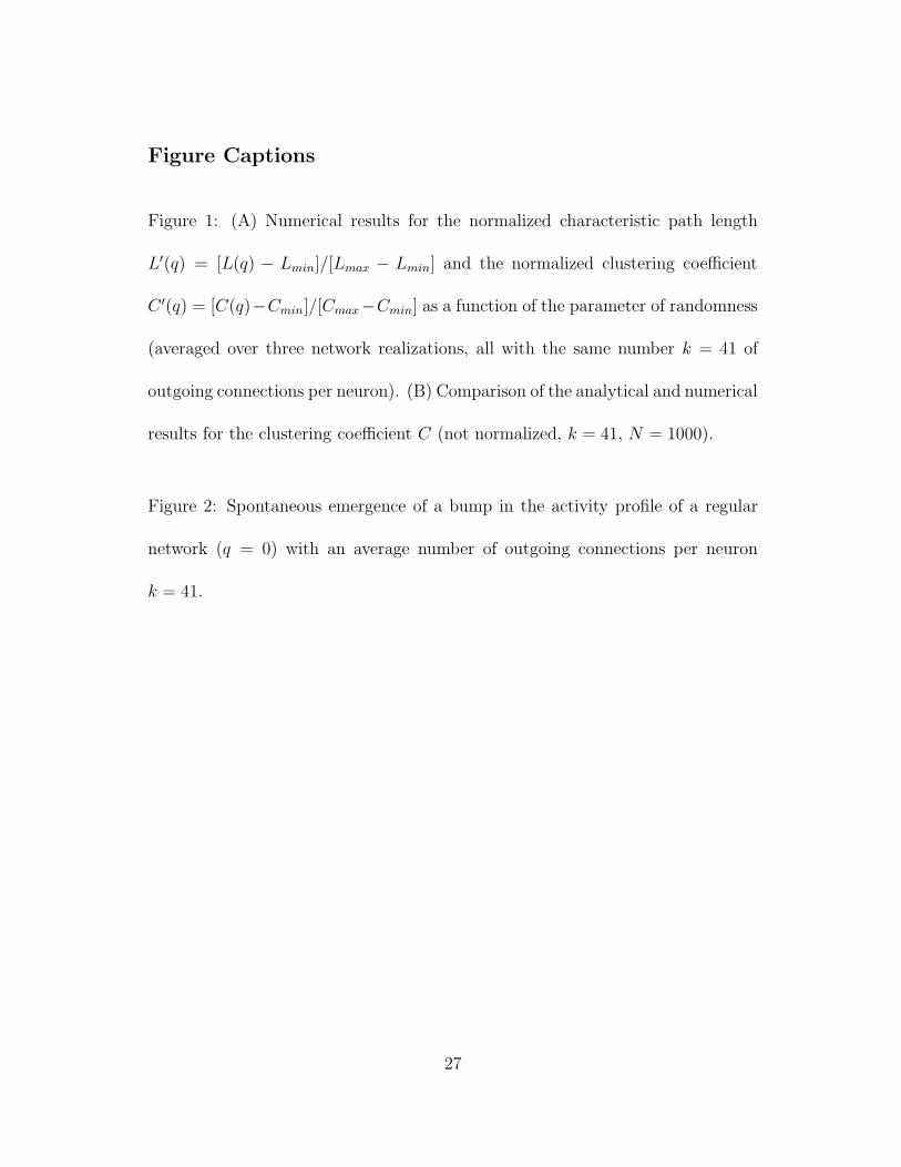
Figure Captions

Figure 1: (A) Numerical results for the normalized characteristic path length

L′(q) = [L(q) − Lmin]/[Lmax − Lmin] and the normalized clustering coefficient

C ′(q) = [C(q)−Cmin]/[Cmax−Cmin] as a function of the parameter of randomness

(averaged over three network realizations, all with the same number k = 41 of

outgoing connections per neuron). (B) Comparison of the analytical and numerical

results for the clustering coefficient C (not normalized, k = 41, N = 1000).

Figure 2: Spontaneous emergence of a bump in the activity profile of a regular

network (q = 0) with an average number of outgoing connections per neuron

k = 41.

27

Figure 3: (A) Activity profiles during the simulation for different values of the

parameter of randomness. Shown is the number of spikes ri (vertical axis) that

each neuron (horizontal axis) has fired in a sliding 50 msec time window. (B)

Overlaps Oµ (vertical axis) of the network activity shown in A with each of the

p = 5 previously stored memory patterns (horizontal axis) - before, during, and

after a 25%-quality cue for the pattern µ = 2 has been given.

Figure 4: Bumpiness of the activity profile (A) and retrieval performance (B) as

a function of the parameter of randomness for three network realizations and the

average (k = 41).

Figure 5: The effect of the cue quality ρ (displayed in the legend) on the retrieval

performance for three network realizations with k = 41 (A - C) and the average

(D). (Note the scale change in D).

Figure 6: The effect of changing the number k of connections per neuron on the

retrieval performance (triangles) and on the bumpiness (dots).

28

0 0.2 0.4 0.6 0.8 10

0.1

0.2

0.3

0.4

0.5

0.6

0.7

0.8

0.9

1

Parameter of randomness

Clu

ster

ing

coef

ficie

nt a

nd p

ath

leng

thA

L (normalized)C (normalized)

0 0.2 0.4 0.6 0.8 10

0.1

0.2

0.3

0.4

0.5

0.6

Parameter of randomness

Clu

stre

ing

coef

ficie

nt

B

Numerical

Analytical

29

0 500 10000

1

2

3

4

5

6

7

8

9

10

0 500 10000

1

2

3

4

5

6

7

8

9

10

0 500 10000

1

2

3

4

5

6

7

8

9

10

0 500 10000

1

2

3

4

5

6

7

8

9

10

Elapsed time:

10 msec

Elapsed time:

15 msec

Elapsed time:

30 msec

Elapsed time:

100 msec

Numb

er of

spike

s

Neuron label Neuron label Neuron label Neuron label

30

Trial Time

q = 0

q = 0.4

q = 0.2

q = 0.6

q = 0.8

q = 1

A

Trial Time

q = 0

q = 0.8

q = 1

q = 0.2

q = 0.4

B

q = 0.6

31

0 0.2 0.4 0.6 0.8 1

0

0.2

0.4

0.6B

Parameter of randomness

Ret

rieva

l per

form

ance

0 0.2 0.4 0.6 0.8 10

0.2

0.4

0.6

A

Parameter of randomness

"Bum

pine

ss"

of th

e ac

tivity

pro

file

Networks

Average

Networks

Average

32

0 0.2 0.4 0.6 0.8 1

0

0.4

0.8

Parameter of randomness

Ret

rieva

l per

form

ance

0 0.2 0.4 0.6 0.8 1

0

0.4

0.8

Parameter of randomness

Ret

rieva

l per

form

ance

0 0.2 0.4 0.6 0.8 1

0

0.4

0.8

Ret

rieva

l per

form

ance

0 0.2 0.4 0.6 0.8 1

0

0.2

0.4

B

Ret

rieva

l per

form

ance

Parameter of randomness

Parameter of randomness Parameter of randomness

Parameter of randomness

A

C D

5 %10 %15 %25 %50 %75 %100 %

33

0 0.5 10

0.2

0.4

0.6

0.8

1

Parameter of randomness

RetrievalBumpiness

0 0.5 10

0.2

0.4

0.6

0.8

1

Parameter of randomness0 0.5 1

0

0.2

0.4

0.6

0.8

1

Parameter of randomness

0 0.5 10

0.2

0.4

0.6

0.8

1

Parameter of randomness0 0.5 1

0

0.2

0.4

0.6

0.8

1

Parameter of randomness0 0.5 1

0

0.2

0.4

0.6

0.8

1

Parameter of randomness

k = 24 k = 57 k = 82

k = 123 k = 166 k = 207

34