Auto-Encoding Variational Bayesrrtammy/DNN/StudentPresentations/AutoEncoderOrZalman.pdf · Diederik...
39
Auto-Encoding Variational Bayes Diederik P Kingma, Max Welling June 18, 2018 Diederik P Kingma, Max Welling Auto-Encoding Variational Bayes June 18, 2018 1 / 39
Transcript of Auto-Encoding Variational Bayesrrtammy/DNN/StudentPresentations/AutoEncoderOrZalman.pdf · Diederik...

Auto-Encoding Variational Bayes
Diederik P Kingma, Max Welling
June 18, 2018
Diederik P Kingma, Max Welling Auto-Encoding Variational Bayes June 18, 2018 1 / 39

Outline
1 Introduction
2 Variational Lower Bound
3 SGVB Estimators
4 AEVB algorithm
5 Variational Auto-Encoder
6 Experiments and results
7 VAE Examples
8 References
Diederik P Kingma, Max Welling Auto-Encoding Variational Bayes June 18, 2018 2 / 39

Introduction
Motivation
Deep learning using Autoencoder shows great success on featureextraction.
Scaling variational inference to large data set.
Approximating the intrtactable posterior can be used for multiplytasks:
RecognitionDenoisingRepresentationVisualiationGenerative Model
Diederik P Kingma, Max Welling Auto-Encoding Variational Bayes June 18, 2018 3 / 39

Introduction
Motivation - Intuition
How to move from our sample xi to latent space zi , and reconstruct x̃i .
Diederik P Kingma, Max Welling Auto-Encoding Variational Bayes June 18, 2018 4 / 39

Introduction
Problem
Intractability: the case where the integral of the marginal likelihoodpθ(x) =
∫pθ(z)pθ(x |z)dz is intractable (we cannot evaluate or
differentiate the marginal likelihood), where the true posterior density
pθ(z |x) = pθ(x |z)pθ(z)oθ(x)
is intractable (so the EM algorithm cannot be
used), and where the required integrals for any reasonable mean-fieldVB algorithm are also intractable.
A large dataset: we have so much data that batch optimization is toocostly; we would like to make parameter updates using smallminibatches or even single datapoints. Sampling based solutions, e.g.Monte Carlo EM, would in general be too slow, since it involves atypically expensive sampling loop per datapoint.
Diederik P Kingma, Max Welling Auto-Encoding Variational Bayes June 18, 2018 5 / 39

Variational Lower Bound
Bayesian inference
θ: Distribution parameters
α: Hyper-parameters of the parameters distribution, e.g. θ ∼ p(θ|α),our prior.
X: Samples
p(X|a) ∼∫p(X|θ)p(θ|α)dθ: Marginal likelihood
p(θ|X, α) ∝ p(X|θ)p(θ|α): Posterior distribution.
MAP -Maximum a posteriori : θ̂MAP(X) = argmax︸ ︷︷ ︸θ
p(X|θ)p(θ|α)
Sample x is sampled by initially sampling θ from θ ∼ p(θ|α), andthen sampling x from x ∼ p(x |θ)
Diederik P Kingma, Max Welling Auto-Encoding Variational Bayes June 18, 2018 6 / 39

Variational Lower Bound
Bayesian inference - Intuition
Let z ∈ θ be an animal generator. with
z ∼ p(α) =
0.3 CatGenerator
0.2 DogGenerator
0.5 ParrotGenerator
Given our sample x = , what is the chances that z is a catgenerator?
p(z = CG |x , α) =p(x |z = CG )p(z = CG |α)∑
Gen∈θ p(x |z = Gen)p(z = Gen|α)
Diederik P Kingma, Max Welling Auto-Encoding Variational Bayes June 18, 2018 7 / 39
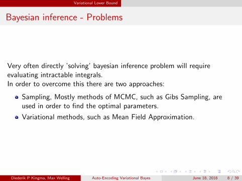
Variational Lower Bound
Bayesian inference - Problems
Very often directly ’solving’ bayesian inference problem will requireevaluating intractable integrals.In order to overcome this there are two approaches:
Sampling, Mostly methods of MCMC, such as Gibs Sampling, areused in order to find the optimal parameters.
Variational methods, such as Mean Field Approximation.
Diederik P Kingma, Max Welling Auto-Encoding Variational Bayes June 18, 2018 8 / 39

Variational Lower Bound
Variational Lower Bound
Instead of evaluating intractable distibution P, we will find a simplerdistribution Q, and use it instead of P where needed:
Diederik P Kingma, Max Welling Auto-Encoding Variational Bayes June 18, 2018 9 / 39

Variational Lower Bound
Variational Lower Bound 1
How can we choose our Q?
Pick some tractable Q which can explain our data well.
Optimize its parameters, using P and our given data.
For example, we could pick Q ∼ N (µ, σ2) and optimize its parametersµ, σ.
Diederik P Kingma, Max Welling Auto-Encoding Variational Bayes June 18, 2018 10 / 39

Variational Lower Bound
Variational Lower Bound 2
Looking at the log probability of the observations X:
logp(X ) = log
∫Zp(X ,Z ) = log
∫Zp(X ,Z )
q(Z )
q(Z )= log(Eq[
p(X ,Z )
q(Z )]) ≥
*Jensen’s inequality
Eq[logp(X ,Z )
q(Z )] = Eq[log(p(X ,Z ))−log(q(Z ))] = Eq[log(p(X ,Z ))]+H(Z )
L = Eq[log(p(X ,Z ))] + H(Z ))
L is the Variational Lower Bound.
Diederik P Kingma, Max Welling Auto-Encoding Variational Bayes June 18, 2018 11 / 39

Variational Lower Bound
Kullback–Leibler divergence
KL Divergence is a measure of how one probability distribution divergesfrom another.
DKL(P||Q) = −∑i
P(i)logQ(i)
P(i)=
∑i
P(i)logP(i)
Q(i)
DKL(P||Q) =
∫P(x)log
P(x)
Q(x)dx
when P(x) = Q(x) for all x ∈ X → DKL(P||Q) = 0DKL(P||Q) is always non-negative.
Diederik P Kingma, Max Welling Auto-Encoding Variational Bayes June 18, 2018 12 / 39

Variational Lower Bound
Variational Lower Bound 3
DKL(q(Z )||p(Z |X )) =
∫q(Z )log
q(Z )
P(Z |X ))dZ = −
∫q(Z )log
P(Z |X )
Q(Z ))dZ =
= −(
∫q(Z )log
p(X ,Z )
q(Z )dZ −
∫q(Z )log(p(X )dZ ) =
= −∫
q(Z )logp(X ,Z )
q(Z )dZ + log(p(X ))
∫q(Z )︸ ︷︷ ︸=1
= −L+ log(p(X )⇒
log(p(X )) = L+ DKL(q(Z )||p(Z |X ))
As KL Divergence is always non negative, we get that log(p(X )) ≥ L, andeither maximizing L or minimizing DKL(q(Z )||p(Z |X )) will optimize q.
Diederik P Kingma, Max Welling Auto-Encoding Variational Bayes June 18, 2018 13 / 39

SGVB Estimators
Stochastic search variational Bayes
Let ψ be distibution q variational parameters. We will want to optimize Lw.r.t both Z (generative parameters) and ψ.Seperate L into Ef and h, where h(X , ψ) contains everything in L exceptfor Ef .
OψL = OψEq[f (z)] + Oψh(X , ψ)
Oψh(X , ψ) is tractable, while for intractable OψEq[f (z)] we willapproximate it using Monte Carlo integration:
OψEq[f (z)] ≈ 1
S
S∑s=1
f (z(s))Oψ ln q(z(s)|ψ)
where z(s) ∼iid q(z |ψ) for s = 1...,S . denote the above approximation asζ. and we recieve the gardient step:
ψt+1 = ψt + ρtOψh(X , ψ(t)) + ρtζt
Diederik P Kingma, Max Welling Auto-Encoding Variational Bayes June 18, 2018 14 / 39

SGVB Estimators
SGVB Estimator
The above method exibits very high variance, may converge very slow, andis impractical for our purpose.We will reparametrize the random variable z̃ ∼ qψ(z |x) using adiffrentiable transformation gψ(ε, x) of an auxilary noise variable ε:
z̃ = gψ(ε, x) with ε ∼ p(ε)
We can now form Monte Carlo estimation of expection of function f (z)w.r.t qψ(z |x):
Eqψ(z|x(i))[f (z)] = Ep(ε)[f (gψ(ε, x (i))] ' 1
S
S∑s=1
f (gψ(ε(s), x (i)))
where ε(s) ∼ p(ε)
Diederik P Kingma, Max Welling Auto-Encoding Variational Bayes June 18, 2018 15 / 39

SGVB Estimators
Estimator A
Applying the above technique to the Variational lower bound L, we yieldour generic SGVB estimator L̃A(θ, ψ; x (i)) ' L(θ, ψ; x (i)):
L̃A(θ, ψ; x (i)) =1
S
S∑s=1
log pθ(x (i), z(i ,s))− log qψ(z(i ,s)|x (i))
where z(i ,l) = gψ(ε(i ,l), x (i)) and ε(l) ∼ p(ε)
Diederik P Kingma, Max Welling Auto-Encoding Variational Bayes June 18, 2018 16 / 39

SGVB Estimators
Estimator B
Alternitivly, we can use the above technique on the KL divergence, therecieve another version of our SGVB estimator:
L̃B(θ, ψ; x (i)) = −DKL(qψ(z |x (i))||pθ(z)) +1
S
S∑s=1
log pθ(x (i)|z(i ,s)))
where z(i ,l) = gψ(ε(i ,l), x (i)) and ε(l) ∼ p(ε)
Diederik P Kingma, Max Welling Auto-Encoding Variational Bayes June 18, 2018 17 / 39

SGVB Estimators
Reparameterization trick - intuition
By adding the noise, we reduce the variance, and pay for it with accuracy:
Diederik P Kingma, Max Welling Auto-Encoding Variational Bayes June 18, 2018 18 / 39

AEVB algorithm
Auto Encoding Variational Bayes
Given multiple data points from data set X with N data points, we canconstruct an estimator of the marginal likelihood of the data set, based onmini-batches:
L(θ, ψ; x (i)) ' L̃M(θ, ψ; xM) =N
M
M∑i=1
L̃(θ, ψ; x (i))
Both estimators A and B can be used.
Diederik P Kingma, Max Welling Auto-Encoding Variational Bayes June 18, 2018 19 / 39

AEVB algorithm
Minibatch AEVB algorithm
1 θ, ψ ← Initialize parameters2 repeat
1 XM ← Random minibatch of M datapoints (drawn from the fulldataset)
2 ε← Random samples from noise distibution p(ε)3 g ← Oψ,θL̃M(θ, ψ;XM , ε) (Gardients of minibatch estimator)4 ψ, θ ← Update parameters using gardients g (SGD or Adagrad)
3 until convergence of parameters θ, ψ
4 Return θ, ψ
Diederik P Kingma, Max Welling Auto-Encoding Variational Bayes June 18, 2018 20 / 39

Variational Auto-Encoder
Variational Auto-Encoder
Variational autoencoders (VAEs) were defined in 2013 by Kingma etal. (This article) and Rezende et al. (Google, simulationsly).
A variational autoencoder consists of an encoder, a decoder, and aloss function:
Diederik P Kingma, Max Welling Auto-Encoding Variational Bayes June 18, 2018 21 / 39
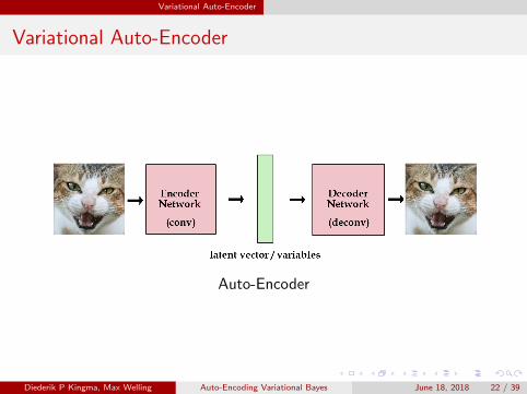
Variational Auto-Encoder
Variational Auto-Encoder
Auto-Encoder
Diederik P Kingma, Max Welling Auto-Encoding Variational Bayes June 18, 2018 22 / 39

Variational Auto-Encoder
Variational Auto-Encoder
Variational Auto-Encoder
Diederik P Kingma, Max Welling Auto-Encoding Variational Bayes June 18, 2018 23 / 39

Variational Auto-Encoder
Variational Auto-Encoder
The encoder is a neural network. Its input is a datapoint x, its outputis a latent (hidden) representation z, and it has weights and biases ψ:
The encoder ‘encodes’ the data which is N-dimensional into a latent(hidden) representation space z which is much less than N dimensions.The lower-dimensional space is stochastic: the encoder outputsparameters to qψ(z |x).
Diederik P Kingma, Max Welling Auto-Encoding Variational Bayes June 18, 2018 24 / 39

Variational Auto-Encoder
Variational Auto-Encoder
The decoder is another neural network. Its input is the representationz , it outputs the parameters to the probability distribution of thedata, and has weights and biases θ:
The decoder outputs parameters to pθ(x |z)The decoder ‘decodes’ the real-valued numbers in z into N real-valuednumbers.
The decoder loosing information. Information is lost because it goesfrom a smaller to a larger dimensionality:
How much information is lost?It measured using the reconstruction log-likelihood log(pθ(x |z)).
Diederik P Kingma, Max Welling Auto-Encoding Variational Bayes June 18, 2018 25 / 39

Experiments and results
Experiments
Using a neural network for our encoder qψ(z |s) (the approximation ofpθ(x , z)).
Optimizing ψ, θ by the AEVB algorithm.
Assume pθ(x |z) is a MV Gaussian/Bernouli, computed from z with aMLP ⇒ pθ(z |x) is intractable.
Let qψ(z |x) be a Gaussian with diagonal covariance:
log qψ(z |x (I )) = logN (z ;µ(i), σ2(i)I )
µ(i), σ2(i)I are outputs of the encoding MLP, i.e. nonlinear functions
of x (i)
Maximizing the objective function:
L(θ, ψ; x (i)) ' 1
2
J∑j=1
(1+log((σ(i)j )2)−µ(i)j
2−σ(i)j
2)+
1
L
L∑l=1
log pθ(x (i)|z(i ,l))
Diederik P Kingma, Max Welling Auto-Encoding Variational Bayes June 18, 2018 26 / 39

Experiments and results
Experiments
Diederik P Kingma, Max Welling Auto-Encoding Variational Bayes June 18, 2018 27 / 39

Experiments and results
Experiments
Trained generative models of images from the MNIST and Frey Facedatasets and compared learning algorithms in terms of the variationallower bound, and the estimated marginal likelihood.
The encoder and decoder have an equal number of hidden units.
For the Frey Face data used decoder with Gaussian outputs, identicalto the encoder, except that the means were constrained to the interval(0,1) using a sigmoidal activation function at the decoder output.
The hidden units are the hidden layer of the neural networks of theencoder and decoder.
Compared performance of AEVB to the wake-sleep algorithm
Diederik P Kingma, Max Welling Auto-Encoding Variational Bayes June 18, 2018 28 / 39

Experiments and results
Experiments
Likelihood lower bound:
Trained generative models (decoders) and corresponding encodershaving 500 hidden units in case of MNIST , and 200 hidden units incase of the Frey Face data.
Marginal likelihood:
For very low-dimensional latent space it is possible to estimate themarginal likelihood of the learned generative models using an MCMCestimator. For the encoder and decoder used neural networks, this timewith 100 hidden units, and 3 latent variables.
Diederik P Kingma, Max Welling Auto-Encoding Variational Bayes June 18, 2018 29 / 39

Experiments and results
Experiments
Comprasion of AEVB method to the wake-sleep algorithm, in terms ofoptimizing the lower bound, for different dimensionality of latent space.
Vertical axis is the estimated avg Variational Lower Bound per data point,Horizontal axis is the amount of training points evaluated
Diederik P Kingma, Max Welling Auto-Encoding Variational Bayes June 18, 2018 30 / 39

Experiments and results
Experiments
Comparison of AEVB to the wake-sleep algorithm and Monte Carlo EM, interms of the estimated marginal likelihood, for a different number of
training points. Monte Carlo EM is not an on-line algorithm, and (unlikeAEVB and the wake-sleep method) can’t be applied efficiently for the full
MNIST dataset.
Diederik P Kingma, Max Welling Auto-Encoding Variational Bayes June 18, 2018 31 / 39

Experiments and results
Experiments
Learned MNIST manifold, on a 2d latent space.
Diederik P Kingma, Max Welling Auto-Encoding Variational Bayes June 18, 2018 32 / 39

VAE Examples
SketchRNN
Schematic of sketch-rnn.
Diederik P Kingma, Max Welling Auto-Encoding Variational Bayes June 18, 2018 33 / 39

VAE Examples
SketchRNN
Latent space interpolations generated from a model trained on pigsketches.
Diederik P Kingma, Max Welling Auto-Encoding Variational Bayes June 18, 2018 34 / 39

VAE Examples
SketchRNN
Learned relationships between abstract concepts, explored using latentvector arithmetic.
Diederik P Kingma, Max Welling Auto-Encoding Variational Bayes June 18, 2018 35 / 39

VAE Examples
MusicVAE
Schematic of MusicVAE
Diederik P Kingma, Max Welling Auto-Encoding Variational Bayes June 18, 2018 36 / 39

VAE Examples
MusicVAE
Beat blender
Diederik P Kingma, Max Welling Auto-Encoding Variational Bayes June 18, 2018 37 / 39

References
References I
Musicvae.https://magenta.tensorflow.org/music-vae.
Teaching machines to draw.https://ai.googleblog.com/2017/04/
teaching-machines-to-draw.html.
Variational autoencoders.https://www.jeremyjordan.me/variational-autoencoders/.
What is variational auto encoder tutorial.https:
//jaan.io/what-is-variational-autoencoder-vae-tutorial/.
B. J. F. Geoffrey E Hinton, Peter Dayan and R. M. Neal.The wakesleep algorithm for unsupervised neural networks.SCIENCE, page 1158–1158, 1995.
Diederik P Kingma, Max Welling Auto-Encoding Variational Bayes June 18, 2018 38 / 39

References
References II
M. I. J. John Paisley, David M. Blei.Variational bayesian inference with stochastic search.ICML, 2012.
C. W. Matthew D Hoffman, David M Blei and J. Paisley.Stochastic variational inference.Journal of Machine Learning Research, 14(1):1303–1347.
D. P.Kingma and M. Welling.Auto-encoding variational bayes.
B. J. P. Simon Duane, Anthony D Kennedy and D. Roweth.Hybrid monte carlo.Physics letters B, 195(2):216–222, 1987.
Diederik P Kingma, Max Welling Auto-Encoding Variational Bayes June 18, 2018 39 / 39


![Continuous Hierarchical Representations with Poincaré ...emilemathieu.fr/PDFs/pvae_poster.pdf · [1]Diederik P. Kingma and Max Welling.Auto-encoding variational bayes.In Proceedings](https://static.fdocuments.in/doc/165x107/5ed408d58d46b66d226352b3/continuous-hierarchical-representations-with-poincar-1diederik-p-kingma.jpg)