Author's personal copy - Universidad de Huelva

(This is a sample cover image for this issue. The actual cover is not yet available at this time.)

This article appeared in a journal published by Elsevier. The attachedcopy is furnished to the author for internal non-commercial researchand education use, including for instruction at the authors institution

and sharing with colleagues.

Other uses, including reproduction and distribution, or selling orlicensing copies, or posting to personal, institutional or third party

websites are prohibited.

In most cases authors are permitted to post their version of thearticle (e.g. in Word or Tex form) to their personal website orinstitutional repository. Authors requiring further information

regarding Elsevier’s archiving and manuscript policies areencouraged to visit:

http://www.elsevier.com/copyright

http://www.elsevier.com/copyright

Author's personal copy

Ecological Modelling 251 (2013) 187– 198

Contents lists available at SciVerse ScienceDirect

Ecological Modelling

jo ur n al homep ag e: www.elsev ier .com/ locate /eco lmodel

Consistency of fuzzy rules in an ecological context

Juan C. Gutiérrez-Estradaa,∗, Inmaculada Pulido-Calvoa, David T. Biltonb

a Dpto. Ciencias Agroforestales, Escuela Técnica Superior de Ingeniería, Campus de La Rábida, Universidad de Huelva, 21819 Palos de la Frontera, Huelva, Spainb Marine Biology and Ecology Research Centre, School of Marine Science and Engineering, University of Plymouth, Drake Circus, Plymouth, PL4 8AA, UK

a r t i c l e i n f o

Article history:Received 16 July 2012Received in revised form12 December 2012Accepted 19 December 2012

Keywords:Evolutionary algorithmWater beetleShannon diversity indexContingencyGeneralized additive models

a b s t r a c t

In this paper, we assess the performance of fuzzy inference systems (FISs) and the consistency of fuzzyrules generated from a meta-analysis exploring diversity–environment relationships, in a system oftemporary and fluctuating ponds located in two regions of southern England. The analyses focus onaquatic coleopteran assemblages, which act as excellent surrogates of wider freshwater macroinverte-brate diversity. Evaluated FISs were calibrated using evolutionary algorithms and the consistency of therules examined using a consistency index specifically developed in this work. The best fit accounted for76% of observed variability in the Shannon diversity index across ponds in the validation phase, whichwas 56 points better than the benchmark value established by a generalized additive model (GAM). Theanalysis of fuzzy rules indicated that the basic dynamics of this system are controlled by 8 rules. Another10 complementary rules were detected, suggesting that more than a single dimension controlled thedynamics of the system. Therefore, water beetle diversity appears to be driven by a relatively short set ofrules which relate diversity and environmental factors in a non-linear manner. These rules can be groupedaccording to their consistency levels, which reflect differences in coleopteran community composition.

© 2013 Elsevier B.V. All rights reserved.

1. Introduction

Ever since Lotfi Zadeh developed his theory of fuzzy sets, thereare many fields of science and engineering in which this theory hasbeen implemented efficiently to solve complex problems (Zadeh,1973; Pappis et al., 1977; Yu et al., 2004). Basically, Zadeh formal-ized mathematically the way in which humans interact with theenvironment. The human mind tends to filter out fuzziness so thatdecisions and actions are more easily made and, therefore, tends toperceive discrete objects and events, distinct boundaries and defi-nite classes of things (Bosserman and Ragade, 1982). These featuresof fuzzy sets theory have clearly been of interest to ecologists, whichexplains the significant increase of applications of this heuristic toecological problems (Meesters et al., 1998; Kampichler et al., 2000;Addriaenssens et al., 2004; Cheung et al., 2005; Mouton et al., 2009).

There are several specific properties that have popularized theuse of fuzzy sets theory among ecologists. The first is that it isan intelligent computational method which does not require avery detailed mathematical description of the process to be ana-lyzed. Generally, these models are easily integrated-implementedin fuzzy logic controllers (FLCs) or fuzzy inference systems (FISs)and utilize a form of many-valued logic. This means that a fuzzy setcan be divided in different regions by mean geometric partitions

∗ Corresponding author. Tel.: +34 959217528; fax: +34 959217528.E-mail address: [email protected] (J.C. Gutiérrez-Estrada).

associated with linguistic concepts which allow us to describe a dis-crete point as a function of its membership to different sets (Zeldisand Prescott, 2000). Other very interesting property of fuzzy setstheory and FISs is that the rules that control the system dynamic canbe grouped and modelled into a defined rule-base as a set of iden-tifiable and comprehensible linguistic labels. In this rule-base (alsoknown as fuzzy associative memory or FAM), a set of antecedentsor premises which also could be interpreted as independent vari-ables (xi), are related with consequents or dependent variables (y)in the following form: Ri = IF x1 is Ai1(x1) and x2 is Ai2(x2) and. . .andxn is Ain(xn), THEN y is Bi(y), where Ai1(x1), Ai2(x2), Ain(xn) and Bi(y)are linguistic concepts, and Ri is the ith rule of the FAM. Therefore,from an ecological point of view, an important advantage of ana-lyzing an ecosystem with fuzzy sets theory is that the informationor knowledge is structured in the form of rules.

However, the knowledge extraction via rules can be an incon-venient in some circumstances. For example, let us suppose that,using an FIS, we are trying to explain the effects of five environmen-tal variables (chemical or physical factors) on the species richnessof a faunistic group. Also, let us suppose that each environmen-tal variable, that is, each independent variable is made up of threefuzzy partitions. This implies that, theoretically, the FAM could havea total of 35 rules (243 rules). In this FAM we could include rulesthat apparently provide contradictory information, which wouldreduce our ability to find an ecological meaning of the variablesimplied in the system. This is particularly common when the FISsare calibrated from real environmental data. Therefore, when we

0304-3800/$ – see front matter © 2013 Elsevier B.V. All rights reserved.http://dx.doi.org/10.1016/j.ecolmodel.2012.12.013


188 J.C. Gutiérrez-Estrada et al. / Ecological Modelling 251 (2013) 187– 198

meta-analyze an ecosystem with FISs, it is not enough to providean FAM. It is also necessary to analyze the consistency of rules, thatis, the absence of contradictory rules in the FAM.

In the literature there are very few works that analyze theconsistency of FAMs and all are focused to engineering applica-tions (Alonso et al., 2008). For example, Jin et al. (1999) proposeda methodology based on evolutionary algorithms for generatingconsistent and compact FAMs for the automatic control of safetydistance in cars. They provided a consistency index calculated as afunction of the similarities of rule premises and rule consequents.On the other hand, Cheong and Lai (2000) used genetic algorithms(GAs) to design FISs for controlling three different industrial plans.These authors used a genetic strategy to obtain an FIS with restric-tions in the FAM. In this way, the number of rules fired at the sametime was minimized to improving the consistency of the FAM. Inboth these works it is assumed that the consistency of the FAMresults in the absence of contradictory rules, in the sense that ruleswith similar premises or antecedents should have similar conse-quent parts (Gacto et al., 2011). In other words, two inconsistentrules will have similar premise parts, but will have rather differentconsequents.

This initial assumption on the consistency of rules could gen-erate erroneous conclusions when we carry out a meta-analysisin an ecological context because unlike engineering problems, theenvironmental data base could be made up of contingent records.Contingency arises when the nature and composition of ecosystemsin different locations are different realizations of the same underly-ing processes (Schmitz, 2010). Therefore, any consistency analysisof rules generated from environmental data must explicitly con-front the issue of contingency. To cope with the above mentionedproblem, a new approach of consistency based on the contingentnature of environmental data is proposed in this paper.

In summary, we use an FIS optimized with evolutionary algo-rithms to extract the set of rules that controls the composition ofa local assemblage. We selected a system which has been previ-ously analyzed, and therefore relatively well studied, providing aset of reference results. The system selected was composed of aseries of temporary and fluctuating ponds in two regions of south-ern England (Lizard and New Forest). In both regions, we focusedour attention on the different diversity patterns of the communityof aquatic Coleopera and their relationships with environmentalfactors. This macroinvertebrate assemblage was selected becausethis group is relatively diverse, ecologically well understood andoccurs across a wide spectrum of pond types (Bilton et al., 2006;Sánchez-Fernández et al., 2006). Evaluation of the accuracy andvalidity of each FIS model was carried out via the comparison oferror levels with those obtained in a reference model, which in ourcase was a generalized additive model (GAM). Finally, the consis-tency of the extracted rules from the best FISs were analyzed withour new approach and compared with existing methodologies.

2. Methods

2.1. Study area and sampling

The dataset used in this study was obtained from 76 tempo-rary ponds located in the New Forest (Hampshire) and the LizardPeninsula (Cornwall), both in southern England. These regionscontain a high density of temporary and fluctuating ponds, dif-fering widely in biological, physical and chemical characteristics.A detailed description of these ecosystems can be found in Biltonet al. (2001), Rundle et al. (2002), Bilton et al. (2006) and Bilton et al.(2009).

Each pond was sampled during February and March 2000, atime when the spatial extent and the presence of ponds were

at their maximum (Bilton et al., 2006). Ponds were sampledusing a hand net (1 mm mesh, dimensions 20 cm × 25 cm), takingsemi-quantitative 1 m sweeps amongst aquatic vegetation. Each1 m sweep involved approximately 10 s of back and forth net-ting over the same area of habitat. This sampling protocol hasbeen favourably evaluated in several investigations on invertebrateassemblages (Rundle et al., 2002; Foggo et al., 2003; Bilton et al.,2006). Two or three such samples were taken from the largest sitesaccording to their area. Sweeps were pooled and samples preservedin 95% ethanol in the field.

In addition, a wide range of environmental variables wasrecorded. Before Coleoptera were sampled pH, temperature com-pensated conductivity and turbidity readings were taken on-siteusing a Solomat 520C probe (Zellweger Analytics, Poole, UK).Water depth in the area sampled was estimated using a 1 mrule (mean of five measurements). For analysis of metal cations(calcium, magnesium, aluminium, nickel, chromium, cobalt, iron,zinc and copper) and nutrient concentrations (organic nitrateand soluble reactive phosphorus), two water samples from eachpond were also collected. However, Gutiérrez-Estrada and Bilton(2010) have previously demonstrated that only four environmentalvariables (conductivity, turbidity, magnesium concentration anddepth) were enough to explain more than 82% of the variation ofwater beetles diversity in New Forest and Lizard regions. Therefore,in this study only these four variables were considered as inputs tothe FIS.

Later, in the laboratory beetles were counted and determinedto species level. Shannon’s index (H′) was calculated for Coleopterafrom each pond following Brower et al. (1998). This diversity mea-sure (the output of the FIS) was selected because it is easy tocalculate and reflects both species richness and the relative abun-dance of species within assemblages. H′ normally varies between1.5 and 3.5, with values higher than 3 being seen as representingdiverse communities whilst those below 2 are relatively uniform(Cowell et al., 2004).

2.2. Fuzzy inference system (FIS)

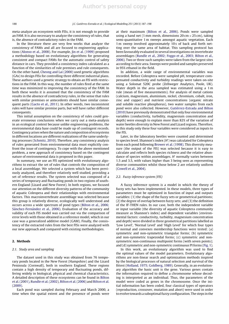
A fuzzy inference system is a model in which the theory offuzzy sets has been implemented. In these models, three types ofparameters must be optimized in function of input and outputsvariables: (1) the shape of the fuzzy sets or geometrical partitions;(2) the degree of overlap between fuzzy sets; and (3) the definitionof the IF-THEN rules. In our case, both the independent variableor input variable (the diversity of aquatic Coleoptera communitymeasure as Shannon’s index) and dependent variables (environ-mental factors: conductivity, turbidity, magnesium concentrationand depth) were divided in three geometrical partitions labelled as‘Low Level’, ‘Normal Level’ and ‘High Level’ for which four typesof normal and convexes membership functions were tested: (a)symmetric and non-symmetric triangular forms; (b) symmetricand non-symmetric trapezoidal forms; (c) symmetric and non-symmetric non-continuous multipoint forms (with seven points);and (d) symmetric and non-symmetric continuous PI forms (Fig. 1).

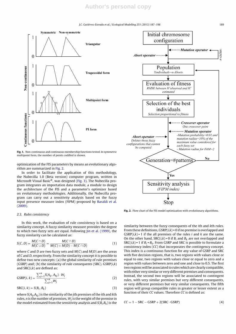
In this work, an evolutionary algorithm was used to findthe optimal values of the model parameters. Evolutionary algo-rithms are non-linear search and optimization methods inspiredby the biological processes of natural selection and survival of thefittest (Holland, 1975; Goldberg, 1989). Generally, in an evolution-ary algorithm the basic unit is the gene. Various genes containthe information required to define a chromosome whose decod-ing is interpreted as an individual. Thus, the parameters of themodel were coded as genes in the chromosome. Once the ini-tial information has been coded, four classical types of operators(reproduction, crossover, mutation and abort) were used in orderto evolve towards a suboptimal fuzzy configuration. The steps in the


J.C. Gutiérrez-Estrada et al. / Ecological Modelling 251 (2013) 187– 198 189

Fig. 1. Non-continuous and continuous membership functions tested. In symmetricmultipoint form, the number of points codified is shown.

optimization of the FIS parameters by means an evolutionary algo-rithm are summarized in Fig. 2.

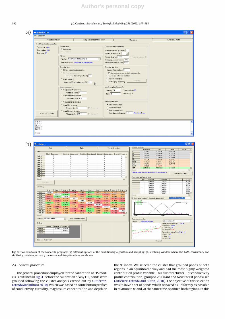
In order to facilitate the application of this methodology,the Nubecilla 1.0 (Beta version) computer program, written inMicrosoft Visual Basic®, was designed (Fig. 3). The Nubecilla pro-gram integrates an importation data module, a module to designthe architecture of the FIS and a parameter’s optimizer basedon evolutionary methodologies. Additionally, the Nubecilla pro-gram can carry out a sensitivity analysis based on the fuzzyinput presence measure index (FIPM) proposed by Baraldi et al.(2009).

2.3. Rules consistency

In this work, the evaluation of rule consistency is based on asimilarity concept. A fuzzy similarity measure provides the degreeto which two fuzzy sets are equal. Following Jin et al. (1999), thefuzzy similarity can be calculated as:

S(C, D) = M(C ∩ D)M(C ∪ D)

= M(C ∩ D)M(C) + M(D) − M(C ∩ D)

(1)

where C and D are two fuzzy sets and M(C) and M(D) are the areasof C and D, respectively. From the similarity concept it is possible todefine two new concepts: (a) the global similarity of rule premises(GSRP) and; (b) the similarity of rule consequents (SRC). GSRP(i,k)and SRC(i,k) are defined as:

GSRP(i, k) =∑n

j=1S(Aij, Akj) · Wj∑nj=1Wj

(2)

SRC(i, k) = S(Bi, Bk) (3)

where S(Aij,Akj) is the similarity of the jth premises of the ith and kthrules, n is the number of premises, Wj is the weight of the premise inthe model estimated from the sensitivity analysis and S(Bi,Bk) is the

Fig. 2. Flow chart of the FIS model optimization with evolutionary algorithms.

similarity between the fuzzy consequents of the ith and kth rules.From these definitions, GSRP(i,k) = 0 if no premise is overlapped andGSRP(i,k) = 1 if the all premises of the rules i and k are the same.On the other hand, SRC(i,k) = 0 if Bi and Bk are not overlapped andSRC(i,k) = 1 if Bi = Bk. From GSRP and SRC is possible to formulate aconsistency index (CC) that incorporates the contingency concept.This index is a continuous function for any value of GSRP and SRCwith five decision regions, that is, two regions with values close orequal to one, two regions with values close or equal to zero and aregion with values between zero and one and close to 0.5. The firsttwo regions will be associated to rules which are clearly compatible,with either very similar or very different premises and consequents.Instead, the second two regions will be associated to contingentrules, with very similar premises but very different consequents,or very different premises but very similar consequents. The fifthregion will group compatible rules in greater or lesser extent as afunction of their CC values. Therefore CC is defined as:

CC = 1 − SRC − GSRP + 2(SRC · GSRP) (4)



Fig. 3. Two windows of the Nubecilla program: (a) different options of the evolutionary algorithm and sampling; (b) evolving window where the FAM, consistency andsimilarity matrixes, accuracy measures and fuzzy functions are shown.

2.4. General procedure

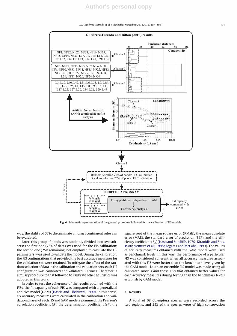
The general procedure employed for the calibration of FIS mod-els is outlined in Fig. 4. Before the calibration of any FIS, ponds weregrouped following the cluster analysis carried out by Gutiérrez-Estrada and Bilton (2010), which was based on contribution profilesof conductivity, turbidity, magnesium concentration and depth on

the H′ index. We selected the cluster that grouped ponds of bothregions in an equilibrated way and had the most highly weightedcontribution profile variable. This cluster (cluster 1 of conductivityprofile contribution) grouped 23 Lizard and New Forest ponds (seeGutiérrez-Estrada and Bilton, 2010). The objective of this selectionwas to have a set of ponds which behaved as uniformly as possiblein relation to H′ and, at the same time, spanned both regions. In this



Fig. 4. Schematic representation of the general procedure followed for the calibration of FIS models.

way, the ability of CC to discriminate amongst contingent rules canbe evaluated.

Later, this group of ponds was randomly divided into two sub-sets: the first one (75% of data) was used for the FIS calibration;the second one (25% remaining, not employed to calculate the FISparameters) was used to validate the model. During the calibration,the FIS configurations that provided the best accuracy measures forthe validation set were retained. To mitigate the effect of the ran-dom selection of data in the calibration and validation sets, each FISconfiguration was calibrated and validated 30 times. Therefore, asimilar procedure to that followed to calibrate other heuristics wasadopted in this work.

In order to test the coherency of the results obtained with theFISs, the fit capacity of each FIS was compared with a generalizedadditive model (GAM) (Hastie and Tibshirani, 1990). In this sense,six accuracy measures were calculated in the calibration and vali-dation phases of each FIS and GAM models examined: the Pearson’scorrelation coefficient (R), the determination coefficient (r2), the

square root of the mean square error (RMSE), the mean absoluteerror (MAE), the standard error of prediction (SEP), and the effi-ciency coefficient (E2) (Nash and Sutcliffe, 1970; Kitanidis and Bras,1980; Ventura et al., 1995; Legates and McCabe, 1999). The valuesof accuracy measures obtained with the GAM model were usedas benchmark levels. In this way, the performance of a particularFIS was considered coherent when all accuracy measures associ-ated with this FIS were better than the benchmark level given bythe GAM model. Later, an ensemble FIS model was made using allcalibrated models and those FISs that obtained better values foreach accuracy measures during testing than the benchmark levelsestablish by GAM model.

3. Results

A total of 68 Coleoptera species were recorded across thetwo regions, and 35% of the species were of high conservation



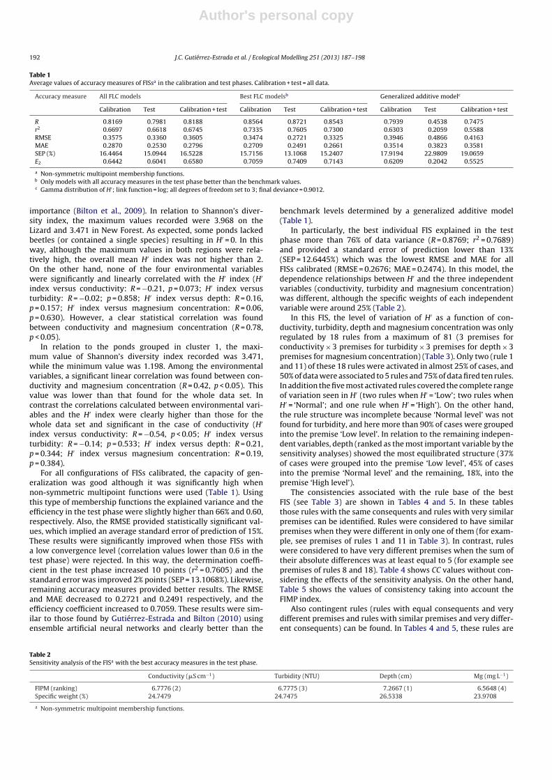
Table 1Average values of accuracy measures of FISsa in the calibration and test phases. Calibration + test = all data.

Accuracy measure All FLC models Best FLC modelsb Generalized additive modelc

Calibration Test Calibration + test Calibration Test Calibration + test Calibration Test Calibration + test

R 0.8169 0.7981 0.8188 0.8564 0.8721 0.8543 0.7939 0.4538 0.7475r2 0.6697 0.6618 0.6745 0.7335 0.7605 0.7300 0.6303 0.2059 0.5588RMSE 0.3575 0.3360 0.3605 0.3474 0.2721 0.3325 0.3946 0.4866 0.4163MAE 0.2870 0.2530 0.2796 0.2709 0.2491 0.2661 0.3514 0.3823 0.3581SEP (%) 16.4464 15.0944 16.5228 15.7156 13.1068 15.2407 17.9194 22.9809 19.0659E2 0.6442 0.6041 0.6580 0.7059 0.7409 0.7143 0.6209 0.2042 0.5525

a Non-symmetric multipoint membership functions.b Only models with all accuracy measures in the test phase better than the benchmark values.c Gamma distribution of H′; link function = log; all degrees of freedom set to 3; final deviance = 0.9012.

importance (Bilton et al., 2009). In relation to Shannon’s diver-sity index, the maximum values recorded were 3.968 on theLizard and 3.471 in New Forest. As expected, some ponds lackedbeetles (or contained a single species) resulting in H′ = 0. In thisway, although the maximum values in both regions were rela-tively high, the overall mean H′ index was not higher than 2.On the other hand, none of the four environmental variableswere significantly and linearly correlated with the H′ index (H′

index versus conductivity: R = −0.21, p = 0.073; H′ index versusturbidity: R = −0.02; p = 0.858; H′ index versus depth: R = 0.16,p = 0.157; H′ index versus magnesium concentration: R = 0.06,p = 0.630). However, a clear statistical correlation was foundbetween conductivity and magnesium concentration (R = 0.78,p < 0.05).

In relation to the ponds grouped in cluster 1, the maxi-mum value of Shannon’s diversity index recorded was 3.471,while the minimum value was 1.198. Among the environmentalvariables, a significant linear correlation was found between con-ductivity and magnesium concentration (R = 0.42, p < 0.05). Thisvalue was lower than that found for the whole data set. Incontrast the correlations calculated between environmental vari-ables and the H′ index were clearly higher than those for thewhole data set and significant in the case of conductivity (H′

index versus conductivity: R = −0.54, p < 0.05; H′ index versusturbidity: R = −0.14; p = 0.533; H′ index versus depth: R = 0.21,p = 0.344; H′ index versus magnesium concentration: R = 0.19,p = 0.384).

For all configurations of FISs calibrated, the capacity of gen-eralization was good although it was significantly high whennon-symmetric multipoint functions were used (Table 1). Usingthis type of membership functions the explained variance and theefficiency in the test phase were slightly higher than 66% and 0.60,respectively. Also, the RMSE provided statistically significant val-ues, which implied an average standard error of prediction of 15%.These results were significantly improved when those FISs witha low convergence level (correlation values lower than 0.6 in thetest phase) were rejected. In this way, the determination coeffi-cient in the test phase increased 10 points (r2 = 0.7605) and thestandard error was improved 2% points (SEP = 13.1068%). Likewise,remaining accuracy measures provided better results. The RMSEand MAE decreased to 0.2721 and 0.2491 respectively, and theefficiency coefficient increased to 0.7059. These results were sim-ilar to those found by Gutiérrez-Estrada and Bilton (2010) usingensemble artificial neural networks and clearly better than the

benchmark levels determined by a generalized additive model(Table 1).

In particularly, the best individual FIS explained in the testphase more than 76% of data variance (R = 0.8769; r2 = 0.7689)and provided a standard error of prediction lower than 13%(SEP = 12.6445%) which was the lowest RMSE and MAE for allFISs calibrated (RMSE = 0.2676; MAE = 0.2474). In this model, thedependence relationships between H′ and the three independentvariables (conductivity, turbidity and magnesium concentration)was different, although the specific weights of each independentvariable were around 25% (Table 2).

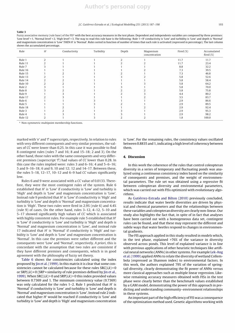
In this FIS, the level of variation of H′ as a function of con-ductivity, turbidity, depth and magnesium concentration was onlyregulated by 18 rules from a maximum of 81 (3 premises forconductivity × 3 premises for turbidity × 3 premises for depth × 3premises for magnesium concentration) (Table 3). Only two (rule 1and 11) of these 18 rules were activated in almost 25% of cases, and50% of data were associated to 5 rules and 75% of data fired ten rules.In addition the five most activated rules covered the complete rangeof variation seen in H′ (two rules when H′ = ‘Low’; two rules whenH′ = ‘Normal’; and one rule when H′ = ‘High’). On the other hand,the rule structure was incomplete because ‘Normal level’ was notfound for turbidity, and here more than 90% of cases were groupedinto the premise ‘Low level’. In relation to the remaining indepen-dent variables, depth (ranked as the most important variable by thesensitivity analyses) showed the most equilibrated structure (37%of cases were grouped into the premise ‘Low level’, 45% of casesinto the premise ‘Normal level’ and the remaining, 18%, into thepremise ‘High level’).

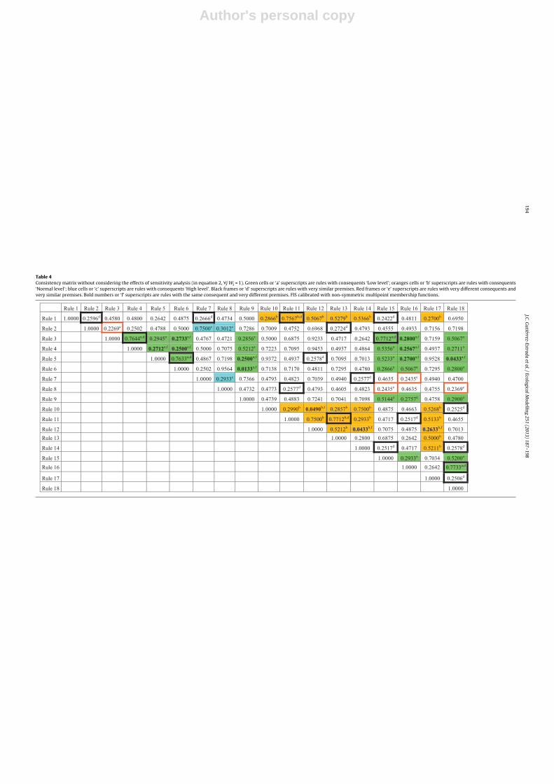
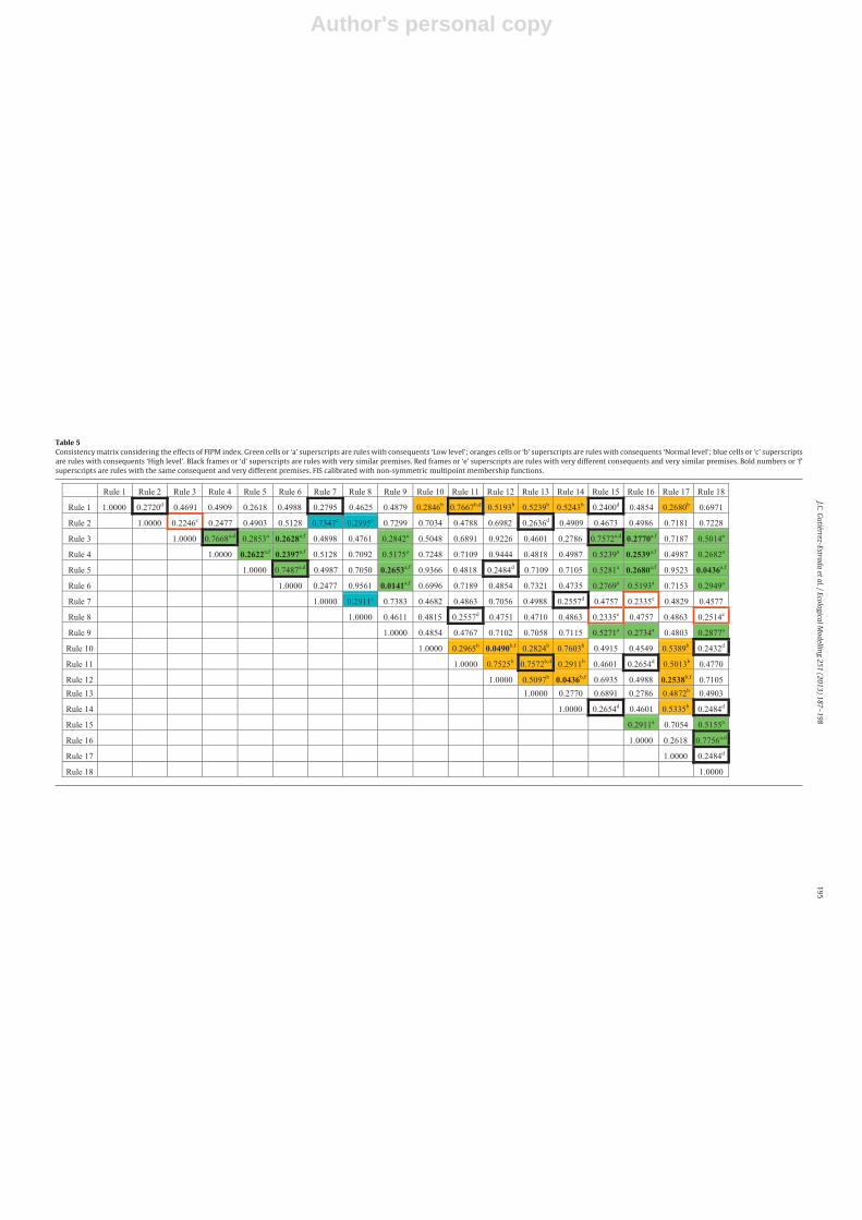
The consistencies associated with the rule base of the bestFIS (see Table 3) are shown in Tables 4 and 5. In these tablesthose rules with the same consequents and rules with very similarpremises can be identified. Rules were considered to have similarpremises when they were different in only one of them (for exam-ple, see premises of rules 1 and 11 in Table 3). In contrast, ruleswere considered to have very different premises when the sum oftheir absolute differences was at least equal to 5 (for example seepremises of rules 8 and 18). Table 4 shows CC values without con-sidering the effects of the sensitivity analysis. On the other hand,Table 5 shows the values of consistency taking into account theFIMP index.

Also contingent rules (rules with equal consequents and verydifferent premises and rules with similar premises and very differ-ent consequents) can be found. In Tables 4 and 5, these rules are

Table 2Sensitivity analysis of the FISa with the best accuracy measures in the test phase.

Conductivity (�S cm−1) Turbidity (NTU) Depth (cm) Mg (mg L−1)

FIPM (ranking) 6.7776 (2) 6.7775 (3) 7.2667 (1) 6.5648 (4)Specific weight (%) 24.7479 24.7475 26.5338 23.9708

a Non-symmetric multipoint membership functions.



Table 3Fuzzy associative memory (rule base) of the FISa with the best accuracy measures in the test phase. Dependent and independents variables are composed by three premises:‘Low level’ = 1, ‘Normal level’ = 2, ‘High level’ = 3. The way to read this rule base is the following: Rule 1 = IF conductivity is ‘Low’ and turbidity is ‘Low’ and depth is ‘Normal’and magnesium concentration is ‘Low’ THEN H′ is ‘Normal’. Rules sorted in function of number of times that each rule is activated (expressed in percentage). The last columnshows the accumulated percentage.

Rule H′ Conductivity Turbidity Depth Magnesiumconcentration

Fired (%) Accumulatedfired (%)

Rule 1 2 1 1 2 1 11.7 11.7Rule 11 2 1 1 2 2 11.7 23.4Rule 7 3 1 1 1 1 8.8 32.2Rule 16 1 1 1 1 2 7.3 39.5Rule 15 1 2 1 2 1 7.3 46.8Rule 13 2 1 1 3 2 5.8 52.6Rule 14 2 2 1 1 1 5.8 58.4Rule 10 2 2 1 1 3 5.8 64.2Rule 2 3 1 1 3 1 5.8 70.0Rule 8 3 2 1 2 2 5.8 75.8Rule 9 1 3 1 2 3 4.4 80.2Rule 17 2 3 1 1 2 3.5 83.7Rule 6 1 1 3 1 1 2.9 86.6Rule 5 1 1 3 2 1 2.9 89.5Rule 18 1 2 1 1 2 2.9 92.4Rule 3 1 2 1 3 1 2.9 95.3Rule 4 1 3 1 3 1 2.9 98.2Rule 12 2 1 3 2 2 1.8 100.0

a Non-symmetric multipoint membership functions.

marked with ‘e’ and ‘f’ superscripts, respectively. In relation to ruleswith very different consequents and very similar premises, the val-ues of CC were lower than 0.25. In this case it was possible to find8 contingent rules (rules 7 and 16; 8 and 15–18; 2 and 3). On theother hand, those rules with the same consequents and very differ-ent premises (superscript ‘f’) had values of CC lower than 0.28. Inthis case the rules implied were: rules 3 and 6–16; 4 and 5–6–16;5 and 9–16–18; 6 and 9, 10 and 12; 12 and 14–17. Between these,the rules 5–18, 12–17, 10–12 and 6–9 had CC values significantlylow.

Rules 6 and 9 were associated with a CC value of 0.0133. There-fore, they were the most contingent rules of the system. Rule 6established that H′ is ‘Low’ if conductivity is ‘Low’ and turbidity is‘High’ and depth is ‘Low’ and magnesium concentration is ‘Low’.Instead rule 9 predicted that H′ is ‘Low’ if conductivity is ‘High’ andturbidity is ‘Low’ and depth is ‘Normal’ and magnesium concentra-tion is ‘High’. These two rules were fired in 2.9% (rule 6) and 4.4%(rule 9) of cases. On the other hand, rules 3–12, 4–12, 5–10 and5–17 showed significantly high values of CC which is associatedwith highly consistent rules. For example rule 5 established that H′

is ‘Low’ if conductivity is ‘Low’ and turbidity is ‘High’ and depth is‘Normal’ and magnesium concentration is ‘Low’, and instead rule17 indicated that H′ is ‘Normal’ if conductivity is ‘High’ and tur-bidity is ‘Low’ and depth is ‘Low’ and magnesium concentration is‘Normal’. In this case the premises were rather different and theconsequents were ‘Low’ and ‘Normal’, respectively. A priori, this isconcordant with the assumption that two rules are consistent ifthey have different premises and consequents, which is in goodagreement with the philosophy of fuzzy set theory.

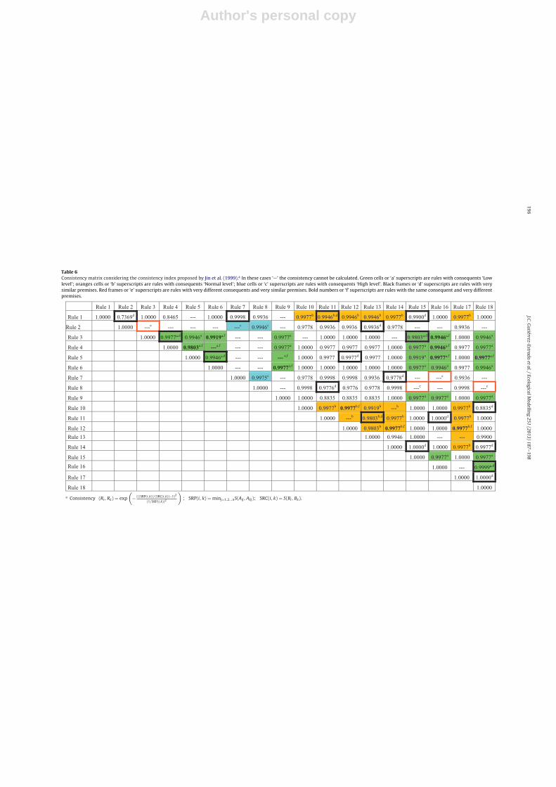
Table 6 shows the consistencies calculated using the indexproposed by Jin et al. (1999). In this matrix it is clear that some con-sistencies cannot be calculated because for these rules SRC(i,k) = 0or SRP(i,k) = 0 (SRP = similarity of rule premises defined by Jin et al.,1999). When SRC(i,k) > 0 and SRP(i,k) > 0 this index provided valuesbetween 0.7369 and 1. The minimum consistency value (0.7369)was only calculated for the rules 1–2. Rule 1 predicted that H′ is‘Normal’ if conductivity is ‘Low’ and turbidity is ‘Low’ and depth is‘Normal’ and magnesium concentration is ‘Low’. Instead rule 2 indi-cated that higher H′ would be reached if conductivity is ‘Low’ andturbidity is ‘Low’ and depth is ‘High’ and magnesium concentration

is ‘Low’. For the remaining rules, the consistency values oscillatedbetween 0.8835 and 1, indicating a high level of coherency betweenthem.

4. Discussion

In this work the coherence of the rules that control coleopterandiversity in a series of temporary and fluctuating ponds was ana-lyzed using a continuous consistency index based on the similarityof consequents and premises, and the weight of environmen-tal parameters. The rule set was obtained using a regressive fitbetween coleopteran diversity and environmental parameters,which was carried out with FISs optimized with evolutionary algo-rithms.

As Gutiérrez-Estrada and Bilton (2010) previously concluded,results indicate that water beetle diversities are driven by phys-ical and chemical parameters and that the relationships betweenthese variables and coleopteran diversity are clearly non-linear. Ourstudy also highlights the fact that, in spite of in fact that analyseshave been carried out with a homogeneous data set, contingentrules can be found, and that these may represent the different andsubtle ways that water beetles respond to changes in environmen-tal gradients.

The FIS approach applied in this study resulted in models which,in the test phase, explained >76% of the variance in diversityobserved across ponds. This level of explained variance is in linewith previous applications of other heuristic techniques like artifi-cial neural networks (ANNs) in other systems. For example Lek-Anget al. (1999) applied ANNs to relate the diversity of wetland Collem-bola (expressed as Shannon index) to environmental factors. Inthis work, the authors explained 79% of the variation of spring-tail diversity, clearly demonstrating the fit power of ANNs versusmore classical approaches such as multiple linear regression. Like-wise remaining accuracy measures obtained with FISs in the testphase were clearly better than the benchmark values establishedby a GAM model, demonstrating the power of this approach in pre-dicting and understanding community–environment relationshipsin these systems.

An important part of the high efficiency of FIS was a consequenceof the optimization method used. Genetic algorithms working with

Author's personal copy194

J.C.

Gutiérrez-Estrada

et

al.

/

Ecological

Modelling

251 (2013) 187– 198

Table 4Consistency matrix without considering the effects of sensitivity analysis (in equation 2, ∀j Wj = 1). Green cells or ‘a’ superscripts are rules with consequents ‘Low level’; oranges cells or ‘b’ superscripts are rules with consequents‘Normal level’; blue cells or ‘c’ superscripts are rules with consequents ‘High level’. Black frames or ‘d’ superscripts are rules with very similar premises. Red frames or ‘e’ superscripts are rules with very different consequents andvery similar premises. Bold numbers or ‘f’ superscripts are rules with the same consequent and very different premises. FIS calibrated with non-symmetric multipoint membership functions.

Rule 1 Rule 2 Rule 3 Rule 4 Rule 5 Rule 6 Rule 7 Rule 8 Rule 9 Rule 10 Rule 11 Rule 12 Rule 13 Rule 14 Rule 15 Rule 16 Rule 17 Rule 18

Rule 1 1.0000 0.25 96d 0.45 80 0.48 00 0.2642 0.4875 0.2666d 0.4734 0.5000 0.2866b 0.7567b,d 0.5067b 0.5279b 0.5366b 0.2422d 0.4811 0.2700b 0.6950

Rule 2 1.00 00 0.22 69e 0.25 02 0.4788 0.5000 0.7500c 0.3012c 0.7286 0.7009 0.4752 0.6968 0.2724d 0.4793 0.4555 0.4933 0.7156 0.7198

Rule 3 1.00 00 0.7644a,d 0.29 45a 0.2733a,f 0.4767 0.4721 0.2856a 0.5000 0.6875 0.9233 0.4717 0.2642 0.7712a,d 0.2800a,f 0.7159 0.5067a

Rule 4 1.00 00 0.27 12a,f 0.2500a,f 0.5000 0.7075 0.5212a 0.7223 0.7095 0.9453 0.4937 0.4864 0.5356a 0.2567a,f 0.4937 0.2711a

Rule 5 1.0000 0.7633a,d 0.4867 0.7198 0.2500a,f 0.9372 0.4937 0.2578d 0.7095 0.7013 0.5233a 0.2700a,f 0.9528 0.0433a,f

Rule 6 1.0000 0.2502 0.9564 0.0133a,f 0.7138 0.7170 0.4811 0.7295 0.4780 0.2866a 0.5067a 0.7295 0.2800a

Rule 7 1.0000 0.2933c 0.7366 0.4793 0.4823 0.7039 0.4940 0.2577d 0.4635 0.2435e 0.4940 0.4700

Rule 8 1.0000 0.4732 0.4773 0.2577d 0.4793 0.4605 0.4823 0.2435e 0.4635 0.4755 0.2369e

Rule 9 1.0000 0.4739 0.4883 0.7241 0.7041 0.7098 0.5144a 0.2757a 0.4758 0.2900a

Rule 10 1.0000 0.2990b 0.0490b,f 0.2857b 0.7500b 0.4875 0.4663 0.5268b 0.2525d

Rule 11 1.0000 0.7500b 0.7712b,d 0.2933b 0.4717 0.2517d 0.5133b 0.4655

Rule 12 1.0000 0.5212b 0.0433b,f 0.7075 0.4875 0.2633b,f 0.7013Rule 13 1.0000 0.2800 0.6875 0.2642 0.5000b 0.4780

Rule 14 1.0000 0.2517d 0.4717 0.5211b 0.2578d

Rule 15 1.0000 0.2933a 0.7034 0.5200a

Rule 16 1.0000 0.2642 0.7733a,d

Rule 17 1.0000 0.2506d

Rule 18 1.0000

Author's personal copyJ.C.

Gutiérrez-Estrada

et

al.

/

Ecological

Modelling

251 (2013) 187– 198195

Table 5Consistency matrix considering the effects of FIPM index. Green cells or ‘a’ superscripts are rules with consequents ‘Low level’; oranges cells or ‘b’ superscripts are rules with consequents ‘Normal level’; blue cells or ‘c’ superscriptsare rules with consequents ‘High level’. Black frames or ‘d’ superscripts are rules with very similar premises. Red frames or ‘e’ superscripts are rules with very different consequents and very similar premises. Bold numbers or ‘f’superscripts are rules with the same consequent and very different premises. FIS calibrated with non-symmetric multipoint membership functions.

Rule 1 Rule 2 Rule 3 Rule 4 Rule 5 Rule 6 Rule 7 Rule 8 Rule 9 Rule 10 Rule 11 Rule 12 Rule 13 Rule 14 Rule 15 Rule 16 Rule 17 Rule 18

Rule 1 1.0000 0.27 20d 0.46 91 0.49 09 0.2618 0.4988 0.2795 0.4625 0.4879 0.2846b 0.7667b,d 0.5193b 0.5239b 0.5243b 0.2400d 0.4854 0.2680b 0.6971

Rule 2 1.00 00 0.22 46e 0.24 77 0.4903 0.5128 0.7347c 0.2995c 0.7299 0.7034 0.4788 0.6982 0.2636d 0.4909 0.4673 0.4986 0.7181 0.7228

Rule 3 1.00 00 0.76 68a,d 0.2853a 0.2628a,f 0.4898 0.4761 0.2842a 0.5048 0.6891 0.9226 0.4601 0.2786 0.7572a,d 0.2770a,f 0.7187 0.5014a

Rule 4 1.00 00 0.2622a,f 0.2397a,f 0.5128 0.7092 0.5175a 0.7248 0.7109 0.9444 0.4818 0.4987 0.5239a 0.2539a,f 0.4987 0.2682a

Rule 5 1.0000 0.7487a,d 0.4987 0.7050 0.2653a,f 0.9366 0.4818 0.2484d 0.7109 0.7105 0.5281a 0.2680a,f 0.9523 0.0436a,f

Rule 6 1.0000 0.2477 0.9561 0.0141a,f 0.6996 0.7189 0.4854 0.7321 0.4735 0.2769a 0.5193a 0.7153 0.2949a

Rule 7 1.0000 0.2911c 0.7383 0.4682 0.4863 0.7056 0.4988 0.2557d 0.4757 0.2335e 0.4829 0.4577

Rule 8 1.0000 0.4611 0.4815 0.2557d 0.4751 0.4710 0.4863 0.2335e 0.4757 0.4863 0.2514e

Rule 9 1.0000 0.4854 0.4767 0.7102 0.7058 0.7115 0.5271a 0.2734a 0.4803 0.2877a

Rule 10 1.0000 0.2965b 0.0490b,f 0.2824b 0.7603b 0.4915 0.4549 0.5389b 0.2432d

Rule 11 1.0000 0.7525b 0.7572b,d 0.2911b 0.4601 0.2654d 0.5013b 0.4770

Rule 12 1.0000 0.5097b 0.0436b,f 0.6935 0.4988 0.2538b,f 0.7105Rule 13 1.0000 0.2770 0.6891 0.2786 0.4872b 0.4903

Rule 14 1.0000 0.2654d 0.4601 0.5335b 0.2484d

Rule 15 0.2911a 0.7054 0.5155a

Rule 16 1.0000 0.2618 0.7756a,d

Rule 17 1.0000 0.2484d

Rule 18 1.0000

Author's personal copy196

J.C.

Gutiérrez-Estrada

et

al.

/

Ecological

Modelling

251 (2013) 187– 198

Table 6Consistency matrix considering the consistency index proposed by Jin et al. (1999).a In these cases ‘—’ the consistency cannot be calculated. Green cells or ‘a’ superscripts are rules with consequents ‘Lowlevel’; oranges cells or ‘b’ superscripts are rules with consequents ‘Normal level’; blue cells or ‘c’ superscripts are rules with consequents ‘High level’. Black frames or ‘d’ superscripts are rules with verysimilar premises. Red frames or ‘e’ superscripts are rules with very different consequents and very similar premises. Bold numbers or ‘f’ superscripts are rules with the same consequent and very differentpremises.

Rule 1 Rule 2 Rule 3 Rule 4 Rule 5 Rule 6 Rule 7 Rule 8 Rule 9 Rule 10 Rule 11 Rule 12 Rule 13 Rule 14 Rule 15 Rule 16 Rule 1 7 Rule 18

Rule 1 1.0000 0.7369d 1.0000 0.8465 --- 1.0000 0.9998 0.9936 --- 0.9977b 0.9946 b,d 0.9946 b 0.9946 b 0.9977 b 0.9900 d 1.0000 0.9977 b 1.0000

Rule 2 1.0000 ---e --- --- --- ---c 0.9946 c --- 0.9778 0.9936 0.9936 0.9936d 0.9778 --- --- 0.9936 ---

Rule 3 1.0000 0.9977ª,d 0.9946a 0.9919ª,f --- --- 0.9977a --- 1.0000 1.0000 1.0000 --- 0.9803 ª,d 0.9946 ª,f 1.0000 0.9946a

Rule 4 1.0000 0.9803a,f ---a,f --- --- 0.9977a 1.0000 0.9977 0.9977 0.9977 1.0000 0.9977 a 0.9946ª,f 0.9977 0.9977a

Rule 5 1.0000 0.9946ª,d --- --- --- a,f 1.0000 0.9977 0.9977 d 0.9977 1.0000 0.9919 a 0.9977ª,f 1.0000 0.9977 ª,f

Rule 6 1.0000 --- --- 0.9977a,f 1.0000 1.0000 1.0000 1.0000 1.0000 0.9977a 0.9946 a 0.9977 0.9946 a

Rule 7 1.0000 0.9975c --- 0.9778 0.9998 0.9998 0.9936 0.9778d --- ---e 0.9936 ---

Rule 8 1.0000 --- 0.9998 0.9776d 0.9776 0.9778 0.9998 ---e --- 0.9998 ---e

Rule 9 1.0000 1.0000 0.8835 0.8835 0.8835 1.0000 0.9977a 0.9977 a 1.0000 0.9977 a

Rule 10 1.0000 0.9977b 0.9977 b,f 0.9919 b ---b 1.0000 1.0000 0.9977 b 0.8835 d

Rule 11 1.0000 ---b 0.9803b, d 0.9977 b 1.0000 1.0000 d 0.9977 b 1.0000

Rule 12 1.0000 0.9803b 0.9977 b,f 1.0000 1.0000 0.9977b,f 1.0000Rule 13 1.0000 0.9946 1.0000 --- --- 0.9900

Rule 14 1.0000 1.0000d 1.0000 0.9977 b 0.9977 d

Rule 15 1.0000 0.9977a 1.0000 0.9977 a

Rule 16 1.0000 --- 0.9999 ª,d

Rule 17 1.0000 1.0000d

Rule 18 1.0000a Consistency (Ri, Rk) = exp

(− (((SRP(i,k))/(SRC(i,k))−1)2

(1/SRP(i,k))2

); SRP(i, k) = minj=1,2...nS(Aij, Akj); SRC(i, k) = S(Bi, Bk).



chromosomes of variable length and coding dependent on thecontext (all of which is possible using the Nubecilla program),allow rapid convergence towards a compact base of fuzzy rules.In this way the data structure analyzed in this work indicated thatcoleopteran diversity in this system was controlled by only 18 rules.From these, only four rules (rules 1, 2, 11 and 7) were associatedwith more than 38% of data set, establishing the basic responseof this community in relation to the environmental variables ana-lyzed. For these four rules, the model predicted that the coleopterandiversity was ‘Normal’ or ‘High’ if conductivity was ‘Low’, turbid-ity was ‘Low’, depth was ‘Normal’, ‘Low’ or ‘High’ and magnesiumconcentration was ‘Low’ or ‘Normal’, which broadly corresponds tocommonly observed responses of lentic macroinvertebrate com-munities to these environmental variables.

The influence of conductivity on macroinvertebrate composi-tion is broadly documented (Kapoor, 1978; Lemly, 1982; Williamset al., 1997; Williams and Williams, 1998; Blasius and Merritt, 2002;Biggs et al., 2005; De Jonge et al., 2008). In the majority of thesestudies a negative relationship between conductivity and richnesswas documented, which is driven by the osmotic challenges mostfreshwater invertebrates face in waters with high ion concentra-tions (Macan, 1974; Blasius and Merritt, 2002). Several studieshave reported that densities and diversity of macroinvertebratesare negatively related with turbidity (Hentges and Stewart, 2010;Hopkins et al., 2011), and likewise depth has been identified asan important direct factor influencing macroinvertebrate commu-nity responses (Muehlbauer et al., 2011), although here responsescould also be related with other co-varying parameters such as theduration of the dry phase (Nicolet et al., 2004). In relation to mag-nesium concentration, it is difficult to provide a direct functionalexplanation, particularly bearing in mind the fact that magne-sium concentration was significantly correlated with conductivity.However, as concluded Gutiérrez-Estrada and Bilton (2010), proxyeffects related with total organic nitrogen (TON) may be importantfor this parameter.

Rules 3, 4, 9 and 18 complemented the basic response. Theserules predicted in an average way that ‘Low’ levels of diversitieswere found when conductivity was ‘High’, turbidity was ‘Low’,depth was ‘Normal-High’ and magnesium concentration was ‘Nor-mal‘, which was coherent with rules 1, 2, 7 and 11. On the otherhand, the remaining rules seem to be consequences of alternativesstrategies that reflect the variety of possible response patterns toenvironmental variations. Several studies have reported that theanimal community found in an individual pond can be significantlydifferent from that in an adjacent pond, despite similar environ-mental conditions (Jeffries, 1989; Jenkins and Buikema, 1998),such differences perhaps reflecting the contingency of coloniza-tion and ‘monopolization’ by early colonists (De Meester et al.,2002). Jeffries (2003) used logistic regressions to analyze the rela-tionships between pond invertebrates and several environmentalfactors, and reported that all variables were significant predictorsof presence–absence of the different species studied for all modelstested, but that no one environmental factor occurred in all mod-els. Jeffries concluded that different species showed alternativelypositive or negative relationships to the same environmental fac-tor, which should be reflected in any model containing differentpredictors of diversity. Likewise, in our study the different diver-sity patterns provided several groups of coherent rules associatedwith different response patterns of H′ to the environmental factorsanalyzed.

Rules 5–18, 6–9, 10–12 and 12–14 showed very low values ofconsistency, denoting high contingency levels. The interactions ofthese rules in a group of ponds with a relatively homogeneousresponse versus coleopteran diversity suggest the existence of dif-ferent environmental scenarios, determined by interactions amongmany factors, rather than that one single dimension controls the

dynamic of this system. This is coherent with one of the prin-cipal thesis of alternative state models theory which establishesthat a system can shift abruptly between two or more states as aconsequence of minor perturbations in environmental conditions(Scheffer et al., 2001). Bilton et al. (2009) reported that ponds inLizard and New Forest regions varied substantially in several bioticand environmental factors like area, depth and vegetation compo-sition, but all were relatively small water bodies, something whichfavours low levels resiliency. Therefore, these rules could be asso-ciated with different hysteresis effects in the collapse or recoveryphases as a consequence of the non-linear behaviour of coleopterandiversity in temporary and fluctuating ponds.

The consistency index proposed in this work has shown its abil-ity to highlight contingent fuzzy rules, even when the rule base hasbeen obtained from an apparently homogeneous data base. Highlycontingent rules take values close to zero whilst rules with a goodlevel of coherence take values close to one. This information com-bined with the percentage of rules fired can help detect differentbehaviours of the estimated variable in relation to the explica-tory variables. Likewise, the CC’s formulation allows the weight ofthe variables to be incorporated into the system, which facilitatesthe interpretation of the rule in the context analyzed. Althoughsome works have dealt the problem of the consistencies of a set offuzzy rules (Jin et al., 1999; Pedrycz, 2003; Alonso et al., 2008), toour knowledge no approach in an ecological context exists in theliterature. In addition, previous works have not considered the con-tingent concept, which implies that for some rules the consistencycannot be calculated, or is barely evaluable. For example, the consis-tency index proposed by Jin et al. (1999) cannot be calculated whenthe similarity between consequents is zero, or it always provideshigh consistency levels when the similarity of premises is very low,independently of the similarity of consequents.

5. Conclusions

In summary, this study has highlighted the non-linear nature ofthe relationship between water beetle diversity and environmen-tal variables in a set of ponds from two regions in the South ofEngland, and demonstrates the strong performance of fuzzy infer-ence systems in modelling diversity–environment interactions.FIS’s generalization capacity (explaining more than 76% of the vari-ance in diversity) suggest that, as with other heuristic techniques,it can be used to simulate the response of organismal diversityunder different environmental scenarios. Also FISs have shownthat a compact and interpretable rule set can be extracted frommeta-analysis of a data set. Finally the consistency index proposedin this work, combined with the percentage of rules fired, allowsthe identification of contingent responses which could illuminateadaptation mechanisms of pond communities to environmentalchanges.

Acknowledgements

Much of the fieldwork which generated the data base of thiswork was conducted under a PhD studentship undertaken by LouiseMcAbendroth. We are grateful to Natural England and the Univer-sity of Plymouth for financial support for this project.

References

Addriaenssens, V., De Baets, B., Goethals, P.L.M., De Pauw, N., 2004. Fuzzy rule-basedmodels for decision support in ecosystem management. The Science of the TotalEnvironment 319, 1–12.

Alonso, J.M., Magdalena, L., Guillaume, S., 2008. HILK: a new methodology ofdesigning highly interpretable linguistic knowledge bases using the fuzzy logicformalism. International Journal of Intelligent Systems 23, 761–794.



Baraldi, P., Librizzi, M., Zio, E., Podofillini, L., Dang, V.N., 2009. Two techniques ofsensitivity and uncertainty analysis of fuzzy expert systems. Expert Systemswith Applications 36, 12461–12471.

Biggs, J., Williams, P., Whitfield, P., Nicolet, P., Weatherby, A., 2005. 15 years of pondassessment in Britain: results and lessons learned from the work of pond conser-vation. Aquatic Conservation: Marine and Freshwater Ecosystems 15, 693–714.

Bilton, D.T., Foggo, A., Rundle, S.D., 2001. Size, permanence and the proportion ofpredators in ponds. Archiv für Hydrobiologie 151, 451–458.

Bilton, D.T., McAbendroth, L.M., Bedford, A., Ramsay, P.M., 2006. How wide to castthe net? Cross-taxon congruence of species richness, community similarity andindicator taxa in ponds. Freshwater Biology 51, 578–590.

Bilton, D.T., McAbendroth, L.C., Nicolet, P., Bedford, A., Rundle, S.D., Foggo, A., Ramsay,P.M., 2009. Ecology and conservation status of temporary and fluctuating pondsin two areas of southern England. Aquatic Conservation: Marine and FreshwaterEcosystems 19, 134–146.

Blasius, B.J., Merritt, R.W., 2002. Field and laboratory investigations on the effectsof road salt (NaCl) on streams macroinvertebrate communities. EnvironmentalPollution 120, 219–231.

Bosserman, R.W., Ragade, R.K., 1982. Ecosystem analysis using fuzzy set theory.Ecological Modelling 16, 191–208.

Brower, J.E., Zar, J.H., von Ende, C.N., 1998. Field and Laboratory Methods for GeneralEcology. McGraw and Hill, Dubuque, IA.

Cheong, F., Lai, R., 2000. Constraining the optimization of a fuzzy logic controllerusing an enhanced genetic algorithm. IEEE Transactions on System, Man andCybernetics Part B: Cybernetics 30, 31–46.

Cheung, W.W.L., Pitcher, T.J., Pauly, D., 2005. A fuzzy logic expert system to esti-mate intrinsic extinction vulnerabilities of marine fishes to fishing. BiologicalConservation 124, 97–111.

Cowell, B.C., Remley, A.H., Lynch, D.M., 2004. Seasonal changes in the distributionand abundance of benthic invertebrates in six headwater streams in centralFlorida. Hydrobiologia 522, 99–115.

De Jonge, M., Van de Vijver, B., Blust, R., Bervoets, L., 2008. Responses of aquaticorganisms to metal pollution in a lowland river in Flandes: a comparisonof diatoms and macroinvertebrates. Science of the Total Environment 407,615–629.

De Meester, L., Gomez, A., Okamura, B., Schwenk, K., 2002. The monopolizationhypothesis and the dispersal-gene flow paradox in aquatic organisms. ActaOecologica 23, 121–135.

Foggo, A., Rundle, S.D., Bilton, D.T., 2003. The net result: evaluating species richnessextrapolations techniques for pond invertebrates. Freshwater Biology 48, 1–9.

Gacto, M.J., Alcalá, R., Herrera, F., 2011. Interpretability of linguistic fuzzy rule-based systems: an overview of terpretability measures. Information Sciences181, 4340–4360.

Goldberg, D., 1989. Genetic Algorithms in Search, Optimization and Machine Learn-ing. Addison Wesley, Reading, MA, USA.

Gutiérrez-Estrada, J.C., Bilton, D.T., 2010. A heuristic approach to predicting waterbeetle diversity in temporary and fluctuating water. Ecological Modelling 221,1451–1462.

Hastie, T.J., Tibshirani, R.J., 1990. Generalized Additive Models. Chapman & Hall/CRC,Boca Raton.

Hentges, A.V., Stewart, T.W., 2010. Macroinvertebrate assemblages in Iowa prairiepothole wetlands and relation to environmental features. Wetlands 30,501–511.

Holland, J., 1975. Adaptation in Natural and Artificial Systems. MIT Press, Cambridge,MA, USA.

Hopkins, J.M., Marcarelli, A.M., Bechtold, H.A., 2011. Ecosystem structure andfunction are complementary measures of water quality in a polluted, spring-influenced river. Water, Air and Soil Pollution 214, 409–421.

Jeffries, M.J., 1989. Measuring Talling’s element of chance in pond populations.Freshwater Biology 21, 383–393.

Jeffries, M.J., 2003. Idiosyncratic relationships between pond invertebrates and envi-ronmental, temporal and patch-specific predictors of incidence. Ecography 26,311–324.

Jenkins, D.G., Buikema, A.L., 1998. Do similar communities develop in similar sites?A test with zooplankton structure and function. Ecological Monograph 68,421–443.

Jin, Y., Von Seelen, W., Sendhoff, B., 1999. On generating FC3 fuzzy rule systemsfrom data using evolution strategies. IEEE Transactions of Systems, Man, andCybernetics 29, 829–845.

Kampichler, C., Barthel, J., Wieland, R., 2000. Species density of foliage-dwellingspiders in field margins: a simple, fuzzy rule-based model. Ecological Modelling129, 87–99.

Kapoor, N.N., 1978. Effect of salinity on the osmoregulatory cells in the tracheal gillsof the stonefly nymph, Paragnetia media (Plecoptera: Perlidae). Canadian Journalof Zoology 56, 2608–2613.

Kitanidis, P.K., Bras, R.L., 1980. Real time forecasting with a conceptual hydro-logical model. 2. Applications and results. Water Resources Research 16 (6),1034–1044.

Legates, D.R., McCabe Jr., G.J., 1999. Evaluating the use of ‘goodness-of-fit’ measuresin hydrologic and hydroclimatic model validation. Water Resources Research 35(1), 233–241.

Lek-Ang, S., Deharverng, L., Lek, S., 1999. Predictive models of collembolandiversity and abundance in a riparian habitat. Ecological Modelling 120,247–260.

Lemly, D.A., 1982. Modification of benthic insect communities in polluted streams:combined effects of sedimentation and nutrient enrichment. Hydrobiologia 87,229–245.

Macan, T.T., 1974. Freshwater Ecology, 2nd ed. Longman Group, London.Meesters, E.H., Bak, R.P.M., Westmacott, S., 1998. A Fuzzy logic model to predict coral

reef development under nutrient and sediment stress. Conservation Biology 12(5), 957–965.

Mouton, A.M., De baets, B., Van Broekhoven, E., Goethals, P.L.M., 2009. Prevalence-adjusted optimisation of fuzzy models for species distribution. EcologicalModelling 15, 1776–1786.

Muehlbauer, J.D., Doyle, M.W., Bernhardt, E.S., 2011. Macroinvertebrate communityresponses to a dewatering disturbance gradient in a restores stream. Hydrologyand Earth System Sciences 15, 1771–1783.

Nash, J.E., Sutcliffe, J.V., 1970. River flow forecasting through conceptual models. I.A discussion of principles. Journal of Hydrology 10, 282–290.

Nicolet, P., Biggs, J., Fox, G., Hodson, M.J., Reynolds, C., Whitfield, M., Williams,P., 2004. The wetland plant and macroinvertebrate assemblages of temporaryponds in England and Wales. Biological Conservation 120, 261–278.

Pappis, C.P., Ebrahim, H., Mamdani, E.H., 1977. Fuzzy logic-controller for a traf-fic junction. IEEE Transactions of Systems, Man, and Cybernetics 7 (10),707–717.

Pedrycz, W., 2003. Expressing relevance interpretability and accuracy of rule-basedsystems. In: Casillas, J., Cordón, O., Herrera, F., Magdalena, L. (Eds.), Inter-pretability Issues in Fuzzy Modeling. Springer-Verlag, Berlin, Heidelberg/NewYork.

Rundle, S.D., Foggo, A., Choisel, V., Bilton, D.T., 2002. Are distribution patterns linkedto dispersal mechanism? An investigation using pond invertebrate assemblages.Freshwater Biology 4, 1571–1581.

Sánchez-Fernández, D., Abellán, P., Mellado, A., Millán, A., Velasco, J., 2006. Are waterbeetles good indicators of biodiversity in Mediterranean aquatic ecosystems?The case of the Segura river basin (SE Spain). Biodiversity and Conservation 15,4507–4520.

Scheffer, M., Carpenter, S., Foley, J.A., Folke, C., Walker, B., 2001. Catastrophic shiftsin ecosystems. Nature 413, 591–596.

Schmitz, O.J., 2010. Resolving Ecosystem Complexity. Monographs in PopulationBiology, vol. 47. Princeton University Press, Oxfordshire, USA.

Ventura, S., Silva, M., Pérez-Bendito, D., Hervás, C., 1995. Artificial neural networksfor estimation of kinetic analytical parameters. Analytical Chemistry 67 (9),1521–1525.

Williams, D.D., Williams, N.E., Cao, Y., 1997. Spatial differences in macroinverte-brates community structure in springs in southeastern Ontario in relation totheir chemical and physical environments. Canadian Journal of Zoology 75,1404–1414.

Williams, D.D., Williams, N.E., 1998. Aquatic insects in an estuarine environ-ment: densities, distribution and salinity tolerance. Freshwater Biology 39,411–421.

Yu, J.Z., Tan, M., Wang, S., 2004. Development of a biomimetic robotic fish and itscontrol algorithm. IEEE Transactions of Systems, Man, and Cybernetics Part B:Cybernetics 34 (4), 1798–1810.

Zadeh, L.A., 1973. Outline of a new approach to the analysis of complex systemsand decision processes. IEEE Transactions of Systems, Man, and Cybernetics 2,28–44.

Zeldis, D., Prescott, S., 2000. Fish disease diagnosis program-problems and somesolutions. Aquacultural Engineering 23, 3–11.

Author's personal copy - Universidad de Huelva

Documents

Transcript of Author's personal copy - Universidad de Huelva