Author's personal copy - Claude Bernard University Lyon...

This article appeared in a journal published by Elsevier. The attachedcopy is furnished to the author for internal non-commercial researchand education use, including for instruction at the authors institution

and sharing with colleagues.

Other uses, including reproduction and distribution, or selling orlicensing copies, or posting to personal, institutional or third party

websites are prohibited.

In most cases authors are permitted to post their version of thearticle (e.g. in Word or Tex form) to their personal website orinstitutional repository. Authors requiring further information

regarding Elsevier’s archiving and manuscript policies areencouraged to visit:

http://www.elsevier.com/copyright

http://www.elsevier.com/copyright

Author's personal copy

Mathematical and Computer Modelling 49 (2009) 2116–2127

Contents lists available at ScienceDirect

Mathematical and Computer Modelling

journal homepage: www.elsevier.com/locate/mcm

A multi-agent model describing self-renewal of differentiation effects onthe blood cell populationNikolai Bessonov a, Ivan Demin b, Laurent Pujo-Menjouet b,∗, Vitaly Volpert ba Institute of Mechanical Engineering Problems, 199178 Saint Petersburg, Russiab Université de Lyon, Université Lyon 1, CNRS, UMR 5208, Institut Camille Jordan, Bâtiment du Doyen Jean Braconnier, 43, blvd du 11 novembre 1918,F - 69222 Villeurbanne Cedex, France

a r t i c l e i n f o

Article history:Received 14 February 2008Accepted 24 July 2008

Keywords:HematopoiesisAnemiaMulti-agent modelSelf-renewalCell communication

a b s t r a c t

In this work, a new multi-agent model is used to describe blood cell population dynamics.More particularly, we focus our simulations here on differentiation and self-renewalprocess based on cell communication. We consider the different cases where progenitorcells are able to self-renew or not in the bone marrow. As a consequence of this study,we give some possible explanations of the mechanism for recovery of the system underimportant blood loss or blood diseases such as anemia.

© 2008 Elsevier Ltd. All rights reserved.

1. Introduction

Hematopoiesis is the blood cell formation that occursmainly in the bonemarrow. Although intensively studied for severaldecades, many open questions remain unanswered, due not only to the complexity of this process, but also to the fact thatmany elements remain impossible to measure experimentally. To contribute to the understanding of this cell development,somemathematical models have been used: stochastic, discrete or deterministic. The first deterministic models for instancehave been initiated in the late 50’s by Lajtha [1], followed by Burns and Tannock [2]. And lately more complex systems havebeen tackled using differential equations or structured partial differential equation describing normal hematopoiesis like[3–6] or blood cell diseases like cyclical neutropenia [7–10], thrombocytopenia [11,12], or chronic myelogenous leukemia[13–17]. However all these models, to the best of our knowledge were quite uneasy to use in biological laboratories. Itwas legitimate then to arise the following question. Is it possible to choose an other method to describe these processes,a method that could be complementary to what has been done, easy to use for biologists and giving results that couldallow to estimate some parameters, predict the dynamics of the population, and simulate a blood disease? A multi-agentmodel appeared then naturally a good solution to this problem. However, it appeared to us that no multi-agent modelseems to have been studied so far for this kind of problem at the cell population dynamics scale. We propose here thento introduce such an approach of the problem and we try to show why it could come out to be quite useful to describehematopoiesis from a cell population point focusing mainly here to the cell communication process. Before this, in the nextsection we shall briefly explain the biological background. Then, in Section 3 we shall introduce the concept of our multi-agent model and show the simulations that could illustrate (Section 4) different cases of self-renewal properties and celldifferentiation.

∗ Corresponding author.E-mail addresses: [email protected] (N. Bessonov), [email protected] (I. Demin), [email protected] (L. Pujo-Menjouet),

[email protected] (V. Volpert).

0895-7177/$ – see front matter© 2008 Elsevier Ltd. All rights reserved.doi:10.1016/j.mcm.2008.07.023


N. Bessonov et al. / Mathematical and Computer Modelling 49 (2009) 2116–2127 2117

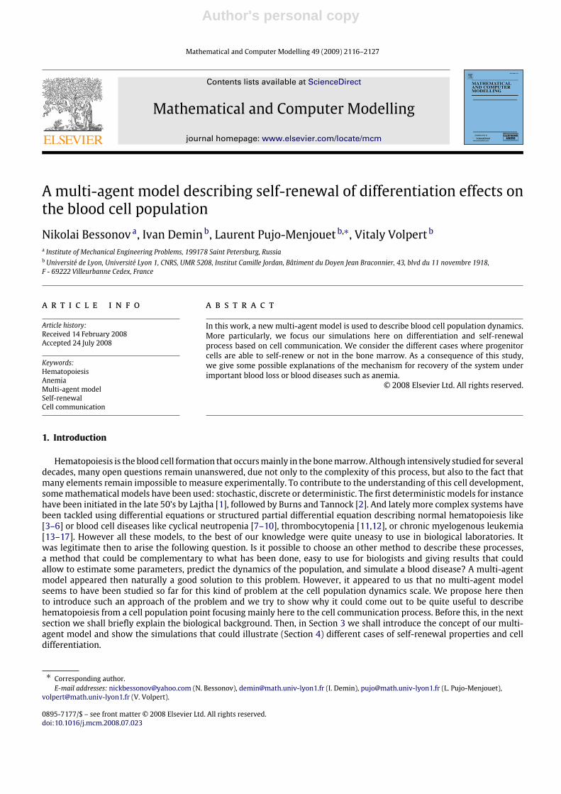
Fig. 1. Scheme of the myeloid lineage formation (red blood cells, platelets and neutrophil cells). A stem cell can divide into either two other stem cells torenew the initial density in case of blood renewal, or one stem cell and one of the three cell types detailed above.

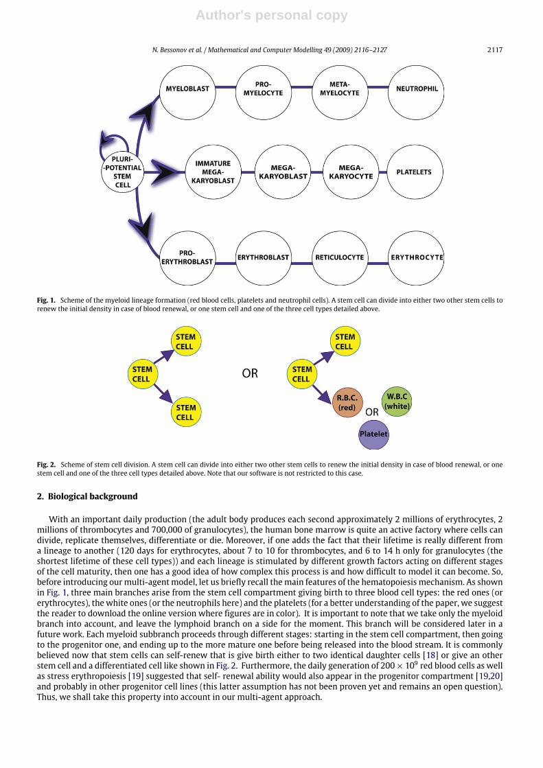
Fig. 2. Scheme of stem cell division. A stem cell can divide into either two other stem cells to renew the initial density in case of blood renewal, or onestem cell and one of the three cell types detailed above. Note that our software is not restricted to this case.

2. Biological background

With an important daily production (the adult body produces each second approximately 2 millions of erythrocytes, 2millions of thrombocytes and 700,000 of granulocytes), the human bone marrow is quite an active factory where cells candivide, replicate themselves, differentiate or die. Moreover, if one adds the fact that their lifetime is really different froma lineage to another (120 days for erythrocytes, about 7 to 10 for thrombocytes, and 6 to 14 h only for granulocytes (theshortest lifetime of these cell types)) and each lineage is stimulated by different growth factors acting on different stagesof the cell maturity, then one has a good idea of how complex this process is and how difficult to model it can become. So,before introducing ourmulti-agentmodel, let us briefly recall themain features of the hematopoiesis mechanism. As shownin Fig. 1, three main branches arise from the stem cell compartment giving birth to three blood cell types: the red ones (orerythrocytes), thewhite ones (or the neutrophils here) and the platelets (for a better understanding of the paper, we suggestthe reader to download the online version where figures are in color). It is important to note that we take only the myeloidbranch into account, and leave the lymphoid branch on a side for the moment. This branch will be considered later in afuture work. Each myeloid subbranch proceeds through different stages: starting in the stem cell compartment, then goingto the progenitor one, and ending up to the more mature one before being released into the blood stream. It is commonlybelieved now that stem cells can self-renew that is give birth either to two identical daughter cells [18] or give an otherstem cell and a differentiated cell like shown in Fig. 2. Furthermore, the daily generation of 200×109 red blood cells as wellas stress erythropoiesis [19] suggested that self- renewal ability would also appear in the progenitor compartment [19,20]and probably in other progenitor cell lines (this latter assumption has not been proven yet and remains an open question).Thus, we shall take this property into account in our multi-agent approach.


2118 N. Bessonov et al. / Mathematical and Computer Modelling 49 (2009) 2116–2127

Fig. 3. Example of what could be considered by the software. The yellow disks represent stem cell, red and blue cells direct offspring of the yellow cells,and light colors their secondary offspring. Yellow (stem) cells are attached to the wall on the left, and all the other cells are pushed away to the right bydivision, and released in the blood systems. (For interpretation of the references to colour in this figure legend, the reader is referred to the web version ofthis article.)

3. The multi-agent model

In order to help the reader to understand the mathematical model behind the software and for clarity, we have put themathematical details in the Appendix. It is also important to keep in mind that many changes can be done when choosingthe parameters of themodel. For instance, it is possible to give the self-renewal ability to all the cells as well as none of them,or to change their lifetime, their size, or their density. As shown in Fig. 3 the blood cells are considered as small disks thatmove away to the right as pushed by the ones dividing. Moremature cells on the right are then released in the blood stream.Amore detailed vision of what the user can see on a computer screen is presented in Fig. 4. One can see on this example thata window is opened where it is possible to choose the different lineages defined by letters (A0, B1, B2, . . . , C1, C2, . . . etc.)corresponding to the cell types and the different maturity levels. Each cell family can have the same color or not, dependingon what one wants to observe. Some obstacles can be added to represent the bone marrow porous structure in a betterway (even if it is still a basic obstacle here and on the way to be improved). Cell size, density, lifetime and the number ofoffspring (up to four, knowing that two is usually way enough for a realistic cell division) can be modified easily. All thedetails are explained in the manual. In Fig. 4 for instance, which could correspond to the myeloid branch described in Fig. 1,we simulated the following scheme:

A0→ A0+ B1+ E1+ F1, B1→ B2+ B2→ B3+ B3→ B4+ B4,E1→ C1+ D1,C1→ C2+ C2→ C3+ C3→ C4+ C4,D1→ D2+ D2→ D3+ D3→ D4+ D4,F1→ F2+ F2→ F3+ F3→ F4+ F4.

In other words, yellow cells (A0 here) are considered as stem cells. They are attached to the left boundary. They are self-renewable, and produce three other cell types, B1, E1, F1. The first step A0→ A0+B1+E1+F1 corresponds to a simplifieddescription of the scheme A0→ A0+B1, A0→ A0+E1, A0→ A0+F1, A0→ A0+A0. Here, a stem cell gives four daughtercells at once instead of dividing four times giving only two daughter cells each time.We understand that it is not biologicallyrealistic to consider such a behavior, but it gives an equivalent qualitative behavior with a simple computing process behind.However, we believe that it could be quite interesting and useful to introduce stochasticity at the stem division level: a stemcell could give then an offspring of a different type with a certain probability. This has not been coded yet but will be a partof our future work. This example is quite simple but has already given good results. It is indeed possible to add somemutantcells (not shown in the figure), with different properties (a faster proliferating rate, an ability to self-renew wherever it islocated, etc.). These ‘‘bad’’ cells could represent leukemic cells developing in the bone marrow in the context of a chronicor acute myeloid leukemia. Description of this phenomenon and simulations with our multi-agent software can be foundin [21].Our objective in the next section is not to go further in leukemia simulations and the impact of malignant cells in the

bonemarrow as presented in [21], but rather the effects of a possible cell ‘‘communication’’ that could occur thanks to somemolecule exchanges between cells. We propose here to give a good insight of this new application as well as some possiblebiological interpretations of the results that we believe are going to be quite useful for the biologists: such as the role ofthe cell cycle duration (fixed or not), the cell size, and molecule exchange parameters between a cell and its neighbors. We



Fig. 4. Example of normal hematopoiesis modeling. Yellow (stem) cells also called A0 can give birth to an other yellow stem cell, or one of the 3 cells (B1,E1, F1), being the origin of the 3 branches (red cells (red), white cells (blue) and platelets (green), respectively). E1 cells can give two sub-branches (whichcan be possible in the myeloid branch, when white cells split into neutrophil, basophil, and the eosinophil branches). These cells differentiate, die or leavethe bone marrow with a certain rate. It is possible in this figure to see that the most mature cells (light colors) are on the right side of the screen. Theycorrespond to the cells leaving the bone marrow as expected. (For interpretation of the references to colour in this figure legend, the reader is referred tothe web version of this article.)

shall see, that it is possible to obtain a cell population behavior close to what is observed in the case of acute myelogenousleukemia without introducing any malignant cells.

4. Cell communication

4.1. Hypotheses behind the software

It is well known now that hematopoiesis is ruled by a complex system of external and internal feedbacks most of thetime by hormone stimulations [22]. It is also believed that blood cells in the bone marrow produce some bio-chemicalmolecules called growth factors that can influence their dynamics and more specifically the differentiation choices forundifferentiated cells. Moreover, it is commonly and adopted idea now that lineage specification which is the process ofcontrolling differentiation of the different lineages is regulated by a system of interacting transcription factors. For instance,in primary erythroblasts, the concentrations of ERK and FASmolecules determine the passage to self-renewal, differentiationor apoptosis process of these cells through an activation cascade and cell to cell molecular exchanges [23]. But the way thissystem is ruled remains not completely elucidated. Some attempts to mathematically describe this process have been doneby Roeder et al. in [24] for two transcription factors. Furthermore, Huang et al. [25]managed to create amodel able to capturesome fundamental features of binary cell fate decisions ‘‘uniting the concepts of stochastic (selective) and deterministic(instructive) regulation’’. Our approach here follows this stream of trying to simulate the lineage specification not onlybetween two sub-populations, but also in the frame of as many populations as decided by the user of our software. Ourobjective for now is not to proceed to a complex analysis as shown in [24,25] but to be able to observe some simulationsthat could give some biologically realistic results – in a qualitative way for the moment, since we are still in the process ofgathering experimental data from different laboratories – with our simple multi-agent model. Then, to investigate whichparameters could get involved at a population level first and not at a molecular level. For the moment, let us keep in mindas said by Glauche et al. in [26] that lineage specification is ‘‘a competition process between different interacting lineagespropensities’’.In order to introduce the problem as clearly as possible, let us consider then the simplest scheme,

A→ A+ B, A→ A+ C .

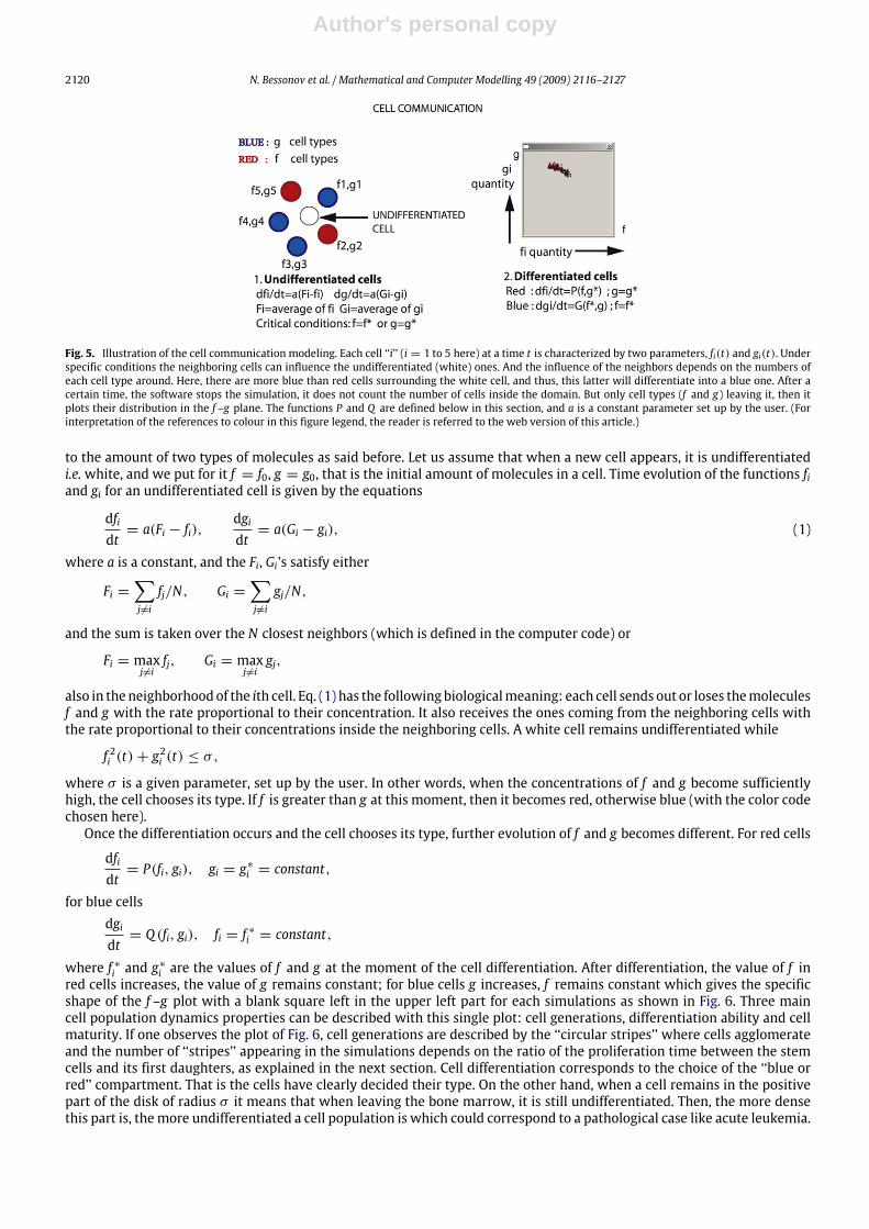
It is possible to complicate this process, but we refer the user to the manual for more complex cases. Here, we specifywhich A-cells choose the first path, that is the B-type, and which ones the second, that is the C-type. Three cell types areconsidered here then: undifferentiated white cells and differentiated red or blue cells (see Fig. 5). Each cell is characterizedby two parameters, f and g such that the ith cell is associated with the functions fi(t) and gi(t), this could refer for instance



Fig. 5. Illustration of the cell communication modeling. Each cell ‘‘i’’ (i = 1 to 5 here) at a time t is characterized by two parameters, fi(t) and gi(t). Underspecific conditions the neighboring cells can influence the undifferentiated (white) ones. And the influence of the neighbors depends on the numbers ofeach cell type around. Here, there are more blue than red cells surrounding the white cell, and thus, this latter will differentiate into a blue one. After acertain time, the software stops the simulation, it does not count the number of cells inside the domain. But only cell types (f and g) leaving it, then itplots their distribution in the f –g plane. The functions P and Q are defined below in this section, and a is a constant parameter set up by the user. (Forinterpretation of the references to colour in this figure legend, the reader is referred to the web version of this article.)

to the amount of two types of molecules as said before. Let us assume that when a new cell appears, it is undifferentiatedi.e.white, and we put for it f = f0, g = g0, that is the initial amount of molecules in a cell. Time evolution of the functions fiand gi for an undifferentiated cell is given by the equations

dfidt= a(Fi − fi),

dgidt= a(Gi − gi), (1)

where a is a constant, and the Fi, Gi’s satisfy either

Fi =∑j6=i

fj/N, Gi =∑j6=i

gj/N,

and the sum is taken over the N closest neighbors (which is defined in the computer code) or

Fi = maxj6=ifj, Gi = max

j6=igj,

also in theneighborhoodof the ith cell. Eq. (1) has the following biologicalmeaning: each cell sends out or loses themoleculesf and g with the rate proportional to their concentration. It also receives the ones coming from the neighboring cells withthe rate proportional to their concentrations inside the neighboring cells. A white cell remains undifferentiated while

f 2i (t)+ g2i (t) ≤ σ ,

where σ is a given parameter, set up by the user. In other words, when the concentrations of f and g become sufficientlyhigh, the cell chooses its type. If f is greater than g at this moment, then it becomes red, otherwise blue (with the color codechosen here).Once the differentiation occurs and the cell chooses its type, further evolution of f and g becomes different. For red cells

dfidt= P(fi, gi), gi = g∗i = constant,

for blue cellsdgidt= Q (fi, gi), fi = f ∗i = constant,

where f ∗i and g∗

i are the values of f and g at the moment of the cell differentiation. After differentiation, the value of f inred cells increases, the value of g remains constant; for blue cells g increases, f remains constant which gives the specificshape of the f –g plot with a blank square left in the upper left part for each simulations as shown in Fig. 6. Three maincell population dynamics properties can be described with this single plot: cell generations, differentiation ability and cellmaturity. If one observes the plot of Fig. 6, cell generations are described by the ‘‘circular stripes’’ where cells agglomerateand the number of ‘‘stripes’’ appearing in the simulations depends on the ratio of the proliferation time between the stemcells and its first daughters, as explained in the next section. Cell differentiation corresponds to the choice of the ‘‘blue orred’’ compartment. That is the cells have clearly decided their type. On the other hand, when a cell remains in the positivepart of the disk of radius σ it means that when leaving the bone marrow, it is still undifferentiated. Then, the more densethis part is, themore undifferentiated a cell population is which could correspond to a pathological case like acute leukemia.



Fig. 6. Cell position in the f –g plane. A white cell remains undifferentiated while f 2i (t) + g2i (t) ≤ σ (inside the disk), where σ is a given parameter

and though the quantity of molecules varies depending on the neighbor cells. f and g vary all the time. However, if the concentrations of f and gbecome sufficiently high (greater than σ ), the cell chooses its type. If f is greater than g at this moment, then it becomes red, otherwise blue (withthe color code chosen here). Once the differentiation occurs and the cell chooses its type, further evolution of f and g becomes different. For red cellsdfi/dt = P(fi, gi), gi = g∗i = constant, for blue cells dgi/dt = Q (fi, gi), fi = f

∗

i = constant. After differentiation, the value of f in red cells increases, thevalue of g remains constant; for blue cells g increases, f remains constant which gives the specific shape of the f − g . (For interpretation of the referencesto colour in this figure legend, the reader is referred to the web version of this article.)

Biologically speaking, this color codingmechanismwouldmean that the cell produces bio-chemical substances accordingto its type only after having reached a certain threshold. We consider quadratic functions P and Q :

P( f , g) = a1 + a2f + a3f 2 + a4fg + a5g, Q ( f , g) = b1 + b2g + b3g2 + b4fg + b5f ,

where ai and bi, i = 1 . . . 5 are some constants defined by the users. This functions are chosen to be quadratic functionsarbitrarily for the sake of simplicity. But, it can be changed anytime by the user. In the next section, we give the results ofseveral simulations showing different kinds of blood cell population behaviors. These behaviors depend on the differentparameters chosen in our software set ups, and they could explain the situations in which cell differentiation, self-renewalproperty, or disease-like patterns occur.

4.2. Illustrations of cell communications

Wewant to describe in this part three main aspects involved in the cell dynamics during hematopoiesis: the influence ofdifferentiation, the cell generations and cell maturity. These three aspects obviously linked in the sense that if cells ‘‘decide’’to differentiate or to self-renew thematurity of the offspringwill not be the same. This would imply different cell generationprofiles and could correspond to either normal hematopoiesis, or a response of the bone marrow due to a severe anemia forinstance. Let us have a good insight first of how the software interface carries out the computations on the screen. As said inthe previous sections, stemcells (undifferentiated) are attached to the left boundary of our domain. These cells produce otherundifferentiated white cells with initial values f = f0, g = g0. When the whole domain is filled with undifferentiated cells,the simulation is stopped. Then, each cell is being prescribed one of the two types, red or blue (with some given values f andg) in a random way. And the simulation starts again. New formed undifferentiated cells now surrounded by differentiatedcells are committed to choose their type under themathematical laws explained in the previous section. This is how, one canobserve that after a certain time, some regions filled by red and blue cells begin to appear showing some layered structuresthat can move, appear or disappear depending on the parameters chosen. Indeed, since the initial distribution is random,two different simulations with the same values of parameters can give different results. In some cases, only one of two celltypes remains, and another disappears completely (not shown here).What is the role of each parameters and functions involved here? We briefly summarize them in the following. As said

before, each cell is characterized by two functions fi and gi that determine its type and its color. We denote by τi themomentof time when the ith cell leaves the computational domain (that is the bone marrow for us). Then the software plots thepoint (fi(τi), gi(τi)) in the (f , g)-plane. If this is done for each cell that leaves the domain, then one can characterize the cellpopulation profiles that reach the blood stream. Let us give some examples representing the main features of our individualbased modeling of cell differentiation. In Fig. 7, it is possible to see the explanations of all the parameters involved in oursimulations. We grouped them into three windows. In window 1, it is possible to modify the choice of the lineage, theproliferation time (exact or not), the area of the domain and the initial amount f0 and g0 of molecules given to a new borncell. In window 2, changes can be done for the ai and bi parameters, i = 1 . . . 5, the choice of the influence of the neighboringcells (mean or max) and the parameter σ . In window 3, the content of each cell leaving the bone marrow is plotted on thef –g plane. In the example of Fig. 7 no self-renewal has been suggested (except for the stem cells A0 with a proliferatingtime shorter than the other cells). Thus, almost no undifferentiated cells are plot in window 3. Moreover, the ‘‘clustering’’



Fig. 7. In addition to the simulations (that is the red and blue cells), three windows open: window 1, 2 and 3. In window 1, the user has set up the lineages(1.1), proliferation time (1.2) with a random choice inside this interval, the radius of the cells (1.3) and the area of the domain (1.4). f0 and g0 are also definedin this window (bottom left). In window 2, the parameters ai and bi , i = 1 . . . 5, the choice of the influence of the neighboring cells (mean or max) and theparameter σ (that is the threshold for which a cell decides to differentiate). Finally, in window 3 appears the plot in the f –g plane of the cells leaving thebone marrow. (For interpretation of the references to colour in this figure legend, the reader is referred to the web version of this article.)

Fig. 8. In this simulation, the only change from Fig. 7 occurs in window 1 andmore precisely in the+/− time column. That is the proliferation time is notexact but distributed. In the plot on the f –g plane one can observe then a less structured differentiated cell distribution.

waves appearing in window 3 suggest the existence of three main cell generations corresponding to the ‘‘maturity’’ level ofcell cohorts. This can be seen on the bone marrow simulations with three different levels of color tones (light red or blue,medium and dark). And as explained in the previous section it corresponds to the ratio between the cell proliferation timeof stem cells and its direct cell daughters’ one, this can be seen in the Window 1, (1.2), first column. In Fig. 7 for instance,the proliferation time for stem cells is set up to be 10 and the daughters’ one is 40, the ratio is then 4, which gives then 4‘‘stripes’’. On the other hand if we change the+/− time column in window 1 as shown in Fig. 8, in other words, if we set arandom choice in the proliferation time interval then one can see that the cell count on the plot of the f –g plane is not aswell separated as in Fig. 7. That is, the three cohorts are not as clear as previously due to the fact that the proliferation timeis distributed while it is exact in Fig. 7, window 1, (1.2), second column.

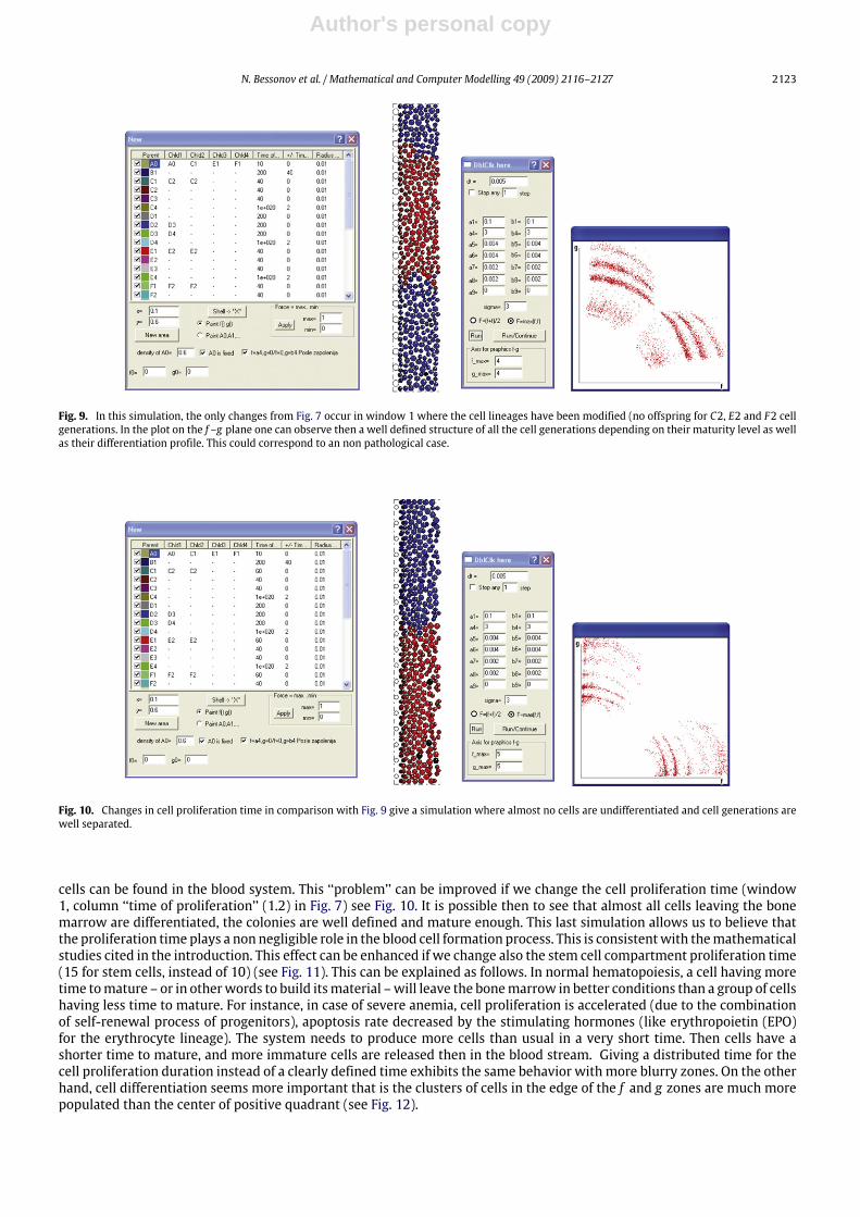
4.2.1. Influence of the cell lineage and proliferation timeNow, let us change the cell lineage in comparison with Fig. 7. That is, we assume that C2, E2 and F2 cells do not

differentiate anymore. Then cell generations are more distinct as seen in Fig. 9 depending on their maturity level. Thiscould correspond to a simplified version of a non pathological case of hematopoiesis, even if a small amount of immature



Fig. 9. In this simulation, the only changes from Fig. 7 occur in window 1 where the cell lineages have been modified (no offspring for C2, E2 and F2 cellgenerations. In the plot on the f –g plane one can observe then a well defined structure of all the cell generations depending on their maturity level as wellas their differentiation profile. This could correspond to an non pathological case.

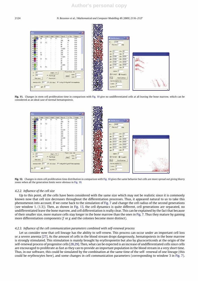
Fig. 10. Changes in cell proliferation time in comparison with Fig. 9 give a simulation where almost no cells are undifferentiated and cell generations arewell separated.

cells can be found in the blood system. This ‘‘problem’’ can be improved if we change the cell proliferation time (window1, column ‘‘time of proliferation’’ (1.2) in Fig. 7) see Fig. 10. It is possible then to see that almost all cells leaving the bonemarrow are differentiated, the colonies are well defined and mature enough. This last simulation allows us to believe thatthe proliferation time plays a non negligible role in the blood cell formation process. This is consistentwith themathematicalstudies cited in the introduction. This effect can be enhanced if we change also the stem cell compartment proliferation time(15 for stem cells, instead of 10) (see Fig. 11). This can be explained as follows. In normal hematopoiesis, a cell having moretime tomature – or in otherwords to build itsmaterial –will leave the bonemarrow in better conditions than a group of cellshaving less time to mature. For instance, in case of severe anemia, cell proliferation is accelerated (due to the combinationof self-renewal process of progenitors), apoptosis rate decreased by the stimulating hormones (like erythropoietin (EPO)for the erythrocyte lineage). The system needs to produce more cells than usual in a very short time. Then cells have ashorter time to mature, and more immature cells are released then in the blood stream. Giving a distributed time for thecell proliferation duration instead of a clearly defined time exhibits the same behavior with more blurry zones. On the otherhand, cell differentiation seems more important that is the clusters of cells in the edge of the f and g zones are much morepopulated than the center of positive quadrant (see Fig. 12).



Fig. 11. Changes in stem cell proliferation time in comparison with Fig. 10 give no undifferentiated cells at all leaving the bone marrow, which can beconsidered as an ideal case of normal hematopoiesis.

Fig. 12. Changes in stem cell proliferation time distribution in comparison with Fig. 10 gives the same behavior but cells are more spread out giving blurryzones when all the generation limits were obvious in Fig. 10.

4.2.2. Influence of the cell sizeUp to this point, all the cells have been considered with the same size which may not be realistic since it is commonly

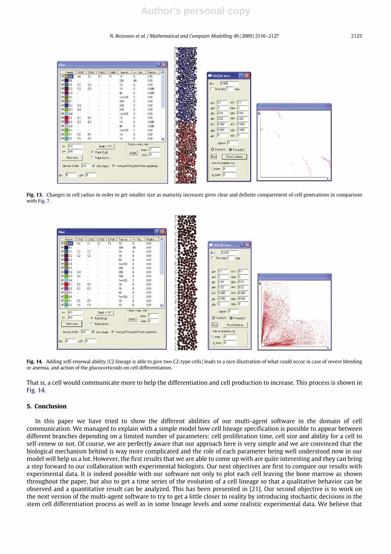
known now that cell size decreases throughout the differentiation processes. Thus, it appeared natural to us to take thisphenomenon into account. If we come back to the simulation of Fig. 7 and change the cell radius of the second generations(see window 1, (1.3)). Then, as shown in Fig. 13, the cell dynamics is quite different, cell generations are separated, noundifferentiated leave the bonemarrow, and cell differentiation is really clear. This can be explained by the fact that becauseof their smaller size, more mature cells stay longer in the bone marrow than the ones in Fig. 7. Thus they mature by gainingmore differentiation components (f or g and the colonies become more distinct).

4.2.3. Influence of the cell communication parameters combined with self-renewal processLet us consider now that cell lineage has the ability to self-renew. This process can occur under an important cell loss

or a severe anemia [27]. As the amount of cells in the blood stream drops dangerously, hematopoiesis in the bone marrowis strongly stimulated. This stimulation is mainly brought by erythropoietin but also by glucocorticoids at the origin of theself-renewal process of progenitor cells [28,29]. Then,what can be expected is an increase of undifferentiated cells since cellsare encouraged to proliferate as fast as they can to provide an important population in the blood stream in a very short time.Thus, in our software, this could be simulated by the combination at the same time of the self- renewal of one lineage (thiscould be erythrocytes here), and some changes in cell communication parameters (corresponding to window 3 in Fig. 7).



Fig. 13. Changes in cell radius in order to get smaller size as maturity increases gives clear and definite compartment of cell generations in comparisonwith Fig. 7.

Fig. 14. Adding self-renewal ability (C2 lineage is able to give two C2-type cells) leads to a nice illustration of what could occur in case of severe bleedingor anemia, and action of the glucocorticoids on cell differentiation.

That is, a cell would communicate more to help the differentiation and cell production to increase. This process is shown inFig. 14.

5. Conclusion

In this paper we have tried to show the different abilities of our multi-agent software in the domain of cellcommunication. We managed to explain with a simple model how cell lineage specification is possible to appear betweendifferent branches depending on a limited number of parameters: cell proliferation time, cell size and ability for a cell toself-renew or not. Of course, we are perfectly aware that our approach here is very simple and we are convinced that thebiological mechanism behind is way more complicated and the role of each parameter being well understood now in ourmodel will help us a lot. However, the first results that we are able to come up with are quite interesting and they can bringa step forward to our collaboration with experimental biologists. Our next objectives are first to compare our results withexperimental data. It is indeed possible with our software not only to plot each cell leaving the bone marrow as shownthroughout the paper, but also to get a time series of the evolution of a cell lineage so that a qualitative behavior can beobserved and a quantitative result can be analyzed. This has been presented in [21]. Our second objective is to work onthe next version of the multi-agent software to try to get a little closer to reality by introducing stochastic decisions in thestem cell differentiation process as well as in some lineage levels and some realistic experimental data. We believe that



our software could appear to be a good tool for biologists in their laboratory to get a good insight of how a cell populationcould behave under administration of some drugs, some malignant cells or other important stress. They could compare itthen with in vivo experiments, and some parameter estimations could come out of their analysis, which for the moment isa challenge for everyone.

Appendix. The model behind the software

Each cell is considered as a disk in the plane. Cells of different types are shownwith different colors (Fig. 3). A cell behavioris characterized by its interactions with other cells, its proliferation, differentiation and apoptosis properties. All this isexplained below.1. Mechanical interaction. Interaction of two neighboring cells is determined by the interaction potential. The sum of

forces acting on each cell from other cells determines the cell motion according to Newton’s law with a possible dampingbecause of the friction with other cells. Thus, we use an approach similar to molecular dynamics simulations even thoughthe potential is different. We have

x′′i − εx′

i +1m

∑i6=j

fij = 0,

where xi is the coordinate of the center of the ith cell,m is itsmass, ε is the damping coefficient, fij is the force acting betweenthe cells i and j. We put

fij = −φ(|xi − xj|),

where the function φ(r, t) equals zero for r ≥ ri + rj and it goes to infinity as r decreases. Here ri and rj are the radii ofthe cells i and j, respectively (which can depend on time). Thus, two cells push each other when the distance between theircenters is less than the sum of their radii.2. Chemical interaction. Cells can produce bio-chemical compounds called growth factors. They can influence behavior of

other cells: apoptosis [22] and possibly differentiation though this still unclear from the biological point of view. We shallcarry out cell modeling taking chemical interactions into account. These interactions are discussed below.3. Cell properties. There can be different cell types in the model. For each type, the user prescribes its behavior, namely,

its lifetime and the type of its offspring in the case of proliferation or differentiation. Let us denote for instance the cell typesby A, B, C here. For each of them a specific lifetime TA, TB, TC is, respectively, prescribed. Actually, it is interesting to notethat each lifetime is not prescribed exactly but with a random interval around its average value. For example, for cells of thetype A it is [TA − τA, TA + τA] with an equal probability inside this interval. When the lifetime of a given cell is over, threepossibilities are offered to it:

1. it dies, that is the corresponding circle is removed from the computational domain (gradually in time, as shown in Fig. 3(‘apoptosis’ arrow)),

2. it differentiates, that is the cell type is changed to another one without changing cell position (it is represented here bya color change)

3. it proliferates, that is the cell is replaced by two other cells. The types of new cells are prescribed by the user. The mothercell grows before dividing, the area of the corresponding circle equals the sum of areas of new circles after the division(this is shown in Fig. 3 (‘stem cell about to divide’ arrow)).

Because the aim of our software was initially to simulate hematopoietic cells in the bone marrow, the example weintroduce below corresponds to blood cell proliferation. It is given in the table of Fig. 4. The user of the software can feel freeto change these conditions depending on what is investigated.The software allows the introduction up to four daughter cells after one division, for example,

A→ A+ B+ C + D, (2)

where A could represent the stem cell, B, C, D the three different lineages (erythrocytes, leukocytes and platelets). Thoughthe cases with three or four cells are not realistic from a biological point of view, it can be convenient for the modeling. Weare currently working on a new version of the software where stochasticity occur at the first division of a stem cell. Therewould be a different probability for this cell to give birth to two stem cells, or either one stem cell and in particular, the lastexample can be considered as an approximation of the scheme

A→ A+ B, A→ C + D. (3)

The scheme (3) implies the introduction of probabilities for each of the two divisions, A→ A+ B and A→ C +D. However,in this work we do not introduce stochastic cell division (it will be considered in the subsequent work).



References

[1] L.G. Lajtha, OnDNA labeling in the study of the dynamics of bonemarrow cell populations, in: F. Stohlman Jr. (Ed.), The Kinetics of Cellular Proliferation,Grune & Stratton, New York, 1959, pp. 173–182.

[2] F.J. Burns, I.F. Tannock, On the existence of a G0 phase in the cell cycle, Cell Tissue Kinet. 3 (1970) 321–334.[3] M. Adimy, L. Pujo-Menjouet, A singular transport model describing cellular division, C.R. Acad. Sci. I-Math. 332 (2001) 1071–1076.[4] M. Adimy, L. Pujo-Menjouet, Asymptotic behavior of a singular transport equation modelling cell division, Discrete Contin. Dyn. Syst. Ser. B 3 (3)(2003) 439–456.

[5] J. Dyson, R. Villella-Bressan, G.F. Webb, A singular transport equation modelling a proliferating maturity structured cell population, Can. Appl. Math.Q. (1996) 65–95.

[6] J. Dyson, R. Villella-Bressan, G.F. Webb, A singular transport equation with delays, Int. J. Math. Math. Sci. 6 (32) (2003) 2011–2026.[7] S. Bernard, J. Blair, M.C. Mackey, Oscillations in cyclical neutropenia: New evidence based on mathematical modeling, J. Theoret. Biol. 223 (2003)283–298.

[8] S. Bernard, J. Blair, M.C. Mackey, Bifurcations in a white blood cell production model, C. R. Biologies 327 (2004) 201–210.[9] C. Haurie, D.C. Dale, M.C. Mackey, Cyclical neutropenia and other periodic hematological diseases: A review ofmechanisms andmathematical models,Blood 92 (1998) 2629–2640.

[10] T. Hearn, C. Haurie, M.C. Mackey, Cyclical neutropenia and the peripheral control of white blood cell production, J. Theoret. Biol. 192 (1998) 167–181.[11] M. Santillan, J. Blair, J.M. Mahaffy, M.C. Mackey, Regulation of platelet production: The normal response to perturbation and cyclical platelet disease,

J. Theoret. Biol. 206 (2000) 585–903.[12] J. Swinburne, M.C. Mackey, Cyclical thrombocytopenia: Characterization by spectral analysis and a review, J. Theoret. Med. 2 (2000) 81–91.[13] M. Adimy, F. Crauste, S. Ruan, Periodic oscillations in leukopoiesis models with two delays, J. Theoret. Biol. 242 (2006) 288–299.[14] M. Adimy, F. Crauste, S. Ruan, A mathematical study of the hematopoiesis process with applications to chronic myelogenous leukemia, SIAM J. Appl.

Math. 65 (4) (2005) 1328–1352.[15] C. Colijn, M.C Mackey, A mathematical model of hematopoiesis: Periodic chronic myelogenous leukemia, part 1, J. Theoret. Biol. 237 (2005) 117–132.[16] M.C. Mackey, C. Ou, L. Pujo-Menjouet, J. Wu, Periodic oscillations of blood cell populations in chronic myelogenous leukemia, SIAM J. Math. Anal. 38

(1) (2006) 166–187.[17] L. Pujo-Menjouet, M.C. Mackey, Contribution to the study of periodic chronic myelogenous leukemia, C.R. Biologies 327 (2004) 235–244.[18] F.M. Watt, B.L. Hogan, Out of eden: Stem cells and their niches, Science 287 (2000) 1427–1430.[19] F. Tronche, O. Wessely, C. Kellendonk, H.M. Reichardt, P. Steinlein, G. Schutz, A. Bauer, H. Beug, The glucocorticoid receptor is required for stress

erythropoiesis, Genes Dev. 13 (22) (1999) 2996–3002.[20] O. Gandrillon, J. Samarut, A. Mey, Un nouveau modèle d’étude de la différenciation érythrocytaire laisse entrevoir une plasticité insoupçonnée des

progéniteurs érythrocytaires, Médecine/Science 15 (1999) 1295–1297.[21] N. Bessonov, L. Pujo-Menjouet, V. Volpert, Cell modelling of hematopoiesis, Mathematical Modelling of Natural Phenomena 1 (2) (2006) 81–103.[22] M.J. Koury, M.C. Bondurant, Erythropoietin retards DNA breakdown and prevents programmed death in erythroid progenitor cells, Science 248 (4953)

(1990) 378–381.[23] C. Rubiolo, D. Piazzola, K. Meissl, H. Beug, J.C. Huber, A. Kolbus, M. Baccarini, A balance between raf-1 and fas expression sets the pace of erythroid

differentiation, Blood 108 (2006) 152–159.[24] I. Roeder, I. Glauche, Towards an understanding of lineage specification in hematopoietic stem cells: A mathematical model for the interaction of

transcription factors gata-1 and pu.1, J. Theoret. Biol. 241 (2006) 852–865.[25] S. Huang, Y-P. Guo, G. May, T. Enver, Bifurcation dynamics in lineage-commitment in bipotent progenitor cells, Develop. Biol. 305 (2007) 695–713.[26] I. Glauche, M. Cross, M. Loeffler, I. Roeder, Lineage specification of hematopoietic stem cells: Mathematical modeling and biological implications, Stem

Cells 25 (7) (2007) 1791–1799.[27] F. Crauste, L. Pujo-Menjouet, S. Génieys, O. Gandrillon, C. Molina, Adding self-renewal in committed erythroid progenitors improves the biological

relevance of a mathematical model of erythropoiesis, J. Theoret. Biol. 250 (2008) 322–338.[28] F. Damiola, C. Keime, S. Gonin-Giraud, S. Dazy, O. Gandrillon, Global transcription analysis of immature avian erythrocytic progenitors: From self-

renewal to differentiation, Oncogene 23 (2004) 7628–7643.[29] S. Dazy, F. Damiola, N. Parisey, H. Beug, O. Gandrillon, The mek-1/ erks signalling pathway is differentially involved in the self-renewal of early and

late avian erythroid progenitor cells, Oncogene 22 (2003) 9205–9216.

Author's personal copy - Claude Bernard University Lyon...

Documents

Transcript of Author's personal copy - Claude Bernard University Lyon...