Author's personal copy - Amir...

This article appeared in a journal published by Elsevier. The attachedcopy is furnished to the author for internal non-commercial researchand education use, including for instruction at the authors institution

and sharing with colleagues.

Other uses, including reproduction and distribution, or selling orlicensing copies, or posting to personal, institutional or third party

websites are prohibited.

In most cases authors are permitted to post their version of thearticle (e.g. in Word or Tex form) to their personal website orinstitutional repository. Authors requiring further information

regarding Elsevier’s archiving and manuscript policies areencouraged to visit:

http://www.elsevier.com/copyright

http://www.elsevier.com/copyright

Author's personal copy

Hydrologic evaluation of satellite precipitation products over a mid-size basin

Ali Behrangi a,b,⇑, Behnaz Khakbaz b, Tsou Chun Jaw b, Amir AghaKouchak b, Kuolin Hsu b,Soroosh Sorooshian b

a Jet Propulsion Laboratory, California Institute of Technology, Pasadena, CA, USAb Center for Hydrometeorology and Remote Sensing (CHRS), The Henry Samueli School of Engineering, Dept. of Civil & Environmental Engineering, University of California,Irvine, CA, USA

a r t i c l e i n f o

Article history:Received 28 May 2010Received in revised form 3 September 2010Accepted 26 November 2010Available online 4 December 2010

This manuscript was handled byK. Georgakakos, Editor-in-Chief, with theassistance of Emmanouil N. Anagnostou,Associate Editor

Keywords:Precipitation estimationRemote sensingHydrologic modelingEvaluation

s u m m a r y

Since the past three decades a great deal of effort is devoted to development of satellite-based precipita-tion retrieval algorithms. More recently, several satellite-based precipitation products have emerged thatprovide uninterrupted precipitation time series with quasi-global coverage. These satellite-based precip-itation products provide an unprecedented opportunity for hydrometeorological applications and climatestudies. Although growing, the application of satellite data for hydrological applications is still very lim-ited. In this study, the effectiveness of using satellite-based precipitation products for streamflow simu-lation at catchment scale is evaluated. Five satellite-based precipitation products (TMPA-RT, TMPA-V6,CMORPH, PERSIANN, and PERSIANN-adj) are used as forcing data for streamflow simulations at 6-hand monthly time scales during the period of 2003–2008. SACramento Soil Moisture Accounting (SAC-SMA) model is used for streamflow simulation over the mid-size Illinois River basin.

The results show that by employing the satellite-based precipitation forcing the general streamflowpattern is well captured at both 6-h and monthly time scales. However, satellites products, with nobias-adjustment being employed, significantly overestimate both precipitation inputs and simulatedstreamflows over warm months (spring and summer months). For cold season, on the other hand, theunadjusted precipitation products result in under-estimation of streamflow forecast. It was found thatbias-adjustment of precipitation is critical and can yield to substantial improvement in capturing bothstreamflow pattern and magnitude. The results suggest that along with efforts to improve satellite-basedprecipitation estimation techniques, it is important to develop more effective near real-time precipitationbias adjustment techniques for hydrologic applications.

� 2010 Elsevier B.V. All rights reserved.

1. Introduction

Precipitation is the key input for hydrometeorological modelingand applications. For accurate flood predictions, reliable quantifi-cation of precipitation data is crucial. However, in many populatedregions of the world including developing countries, ground-basedmeasurement networks (whether from radar or rain gauge) areeither sparse in both time and space or nonexistent. This situationrestricts these regions to manage water resources and hampersearly flood warning systems resulting in massive socioeconomicdamages.

With suites of sensors flying on a variety of satellites over thelast three decades, many satellite-based precipitation estimationalgorithms have been developed to make the precipitation dataavailable to the community in quasi-global scale. Several high

resolution precipitation products are now operational in high res-olution at quasi-global scale. Among those are the TRMM Multi-satellite Precipitation Analysis (TMPA; Huffman et al., 2007), thePrecipitation Estimation from Remotely Sensed Information UsingArtificial Neural Networks (PERSIANN; Hsu et al., 1997; Sorooshianet al., 2000), Climate Prediction Center (CPC) morphing algorithm(CMORPH; Joyce et al., 2004), and the Naval Research LaboratoryGlobal Blended-Statistical Precipitation Analysis (NRLgeo; Turket al., 2000). Although different in the precipitation estimation pro-cedure, in all of the listed products a combination of informationfrom infrared and microwave sensors on geostationary and lowearth orbiting satellites are used in attempt to improve the consis-tency, accuracy, coverage, and timeliness of high resolution precip-itation data.

Given different estimation techniques and the existing uncer-tainties in retrieving precipitation characteristics from satelliteinformation (Krajewski et al., 2000; Adler et al., 2001; Ebertet al., 2007; Gottschalck et al., 2005; AghaKouchak et al., 2009;McCollum et al., 2002; Tian et al., 2007), studies on reliability ofhydrologic predictions based on the satellite-derived precipitation

0022-1694/$ - see front matter � 2010 Elsevier B.V. All rights reserved.doi:10.1016/j.jhydrol.2010.11.043

⇑ Corresponding author at: Jet Propulsion Laboratory, California Institute ofTechnology, 4800 Oak Grove Drive, MS 183-301, Pasadena, CA 91109, USA. Tel.: +1949 3023688.

E-mail address: [email protected] (A. Behrangi).

Journal of Hydrology 397 (2011) 225–237

Contents lists available at ScienceDirect

Journal of Hydrology

journal homepage: www.elsevier .com/ locate / jhydrol


data need to be continued. One useful feedback of such studies is toassess the applicability of satellite-based streamflow prediction fordata sparse regions. These types of studies are also motivated byglobal decline of in situ networks for hydrologic measurements(Stokstad, 1999; Shiklomanov et al., 2002) as opposed to the grow-ing trend in the availability of satellite sensors providing more fre-quent and more accurate precipitation-relevant information andalso near future mission such as the Global Precipitation Measure-ment (GPM) missions among others. In concert with such develop-ments, great deals of research are being conducted to improvequality and resolution of precipitation products from individualor combination of sensors (e.g., Behrangi et al., 2010b amongothers).

Several previous studies estimated streamflow by using hydro-logic models with inputs obtained from remotely sensed data(Hong et al., 2006; Hossain and Anagnostou, 2004; Yilmaz et al.,2005). Schultz (1996) proposed a model to reconstruct monthlyrunoff estimates based on the geostationary satellite data, and ap-plied a hydrologic model to obtain flood hydrographs. Tsintikidiset al. (1999) evaluated the feasibility of satellite-derived meanareal precipitation estimates for hydrologic application acrossnorthern Africa. Using Meteosat inferred precipitation data Grimesand Diop (2003) predicted streamflow estimates and concludedthat inclusion of numerical weather model outputs might improvethe estimated flood hydrographs. Nijssen and Lettenmaier (2004)investigated the effect of satellite-based precipitation sampling er-ror on estimated hydrological fluxes. Using TMPA data, Su et al.,2008 investigated the feasibility of satellite-based precipitationdata for hydrologic predictions. They concluded that satellite esti-mates have potential for hydrologic forecasting particularly withrespect to simulation of seasonal and inter-annual stream-flowvariability.

This study aims to assess the use of available near real-timeoperational precipitation estimation products in streamflow fore-casting. The objective of present study is threefold. First, how doesprecipitation estimation from satellite data using different algo-rithms and ground multi-sensor product compare at a mid-range

size basin. Second, assuming that the hydrologic model generatesreliable streamflow estimations, how differences in input precipi-tation characteristics among different products are reflected inresulting streamflow hydrographs at the time scale (usually 6 h)used by the NWS. The results provide insights on needed accuracyfor precipitation input. Finally, evaluation of precipitation inputswith respect to ground-based streamflow observations at wa-tershed outlet can provide a secondary check, particularly forhydrologic applications.

The paper consists of 5 sections. In Section 2, case study speci-fications including period and area of study, description of hydro-logic model, and datasets are provided. Method and modelcalibration are described in Section 3. Section 4 outlines the resultsand discussion of findings. Finally, concluding remarks are pre-sented in Section 5.

2. Case study specifications

2.1. Period and area of study

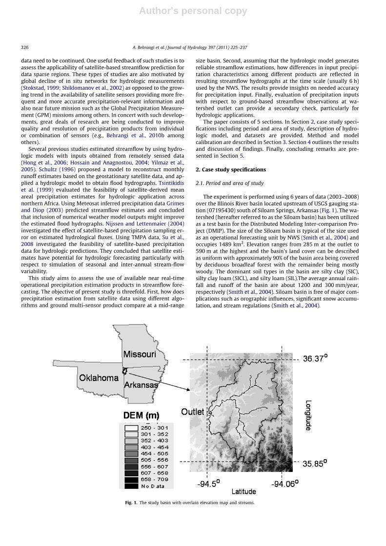
The experiment is performed using 6 years of data (2003–2008)over the Illinois River basin located upstream of USGS gauging sta-tion (07195430) south of Siloam Springs, Arkansas (Fig. 1). The wa-tershed (hereafter referred to as the Siloam basin) has been utilizedas a test basin for the Distributed Modeling Inter-comparison Pro-ject (DMIP). The size of the Siloam basin is typical of the size usedas an operational forecasting unit by NWS (Smith et al., 2004) andoccupies 1489 km2. Elevation ranges from 285 m at the outlet to590 m at the highest and the basin’s land cover can be describedas uniform with approximately 90% of the basin area being coveredby deciduous broadleaf forest with the remainder being mostlywoody. The dominant soil types in the basin are silty clay (SIC),silty clay loam (SICL), and silty loam (SIL).The average annual rain-fall and runoff of the basin are about 1200 and 300 mm/year,respectively (Smith et al., 2004). Siloam basin is free of major com-plications such as orographic influences, significant snow accumu-lation, and stream regulations (Smith et al., 2004).

Fig. 1. The study basin with overlain elevation map and streams.

226 A. Behrangi et al. / Journal of Hydrology 397 (2011) 225–237


2.2. Description of the hydrologic model

The SACramento Soil Moisture Accounting (SAC-SMA) (Burnashet al., 1973; Burnash, 1995) is used to model the rainfall–runoffprocess. SAC-SMA is a lumped, conceptual model and is being usedas the core component of the National Weather Service (NWS)River Forecasting System (NWSRFS) for rainfall-runoff modelingat the basin scale. Mean Areal Precipitation (MAP) and potentialevapotranspiration are forcing data for the model to generate run-off response components. The model consists of an upper-zonerepresenting the uppermost soil layer and a lower-zone represent-ing the deeper portion of the soil profile. Each zone includes ten-sion and free water storages. Depending on the status of theupper-zone free water and the deficiencies in the lower-zone sto-rages, the percolation rate from the upper to the lower layer is con-trolled through a non-linear process. The model has sixteenparameters and six soil moisture states and generates five runoffresponse components as following: (1) direct runoff resulted fromfalling precipitation on permanent and temporary imperviousareas, (2) surface runoff generated when the precipitation rate isgreater than percolation rate, (3) interflow, which is the lateral out-flow from the upper-zone free water storage, (4) supplementarybase flow, which is the lateral drainage from lower-zone supple-mentary free water storage, and (5) primary base flow, which isthe lateral drainage from the lower-zone primary free water stor-age. The summation of runoff components is then convolved withthe unit-hydrograph of the basin’s outlet to generate thestreamflow at this location.

2.3. Datasets

The dataset used in this study consists of precipitation forcingfrom five satellite-based products along with the reference groundmulti-sensor precipitation data, potential evaporation, and stream-flow observations at basin’s outlet. The satellite-derived precipita-tion products utilized in the present study are: (1) TMPA real-time(hereafter referred to as TMPA-RT), collecting available micro-wave-derived precipitation estimates from various satellites with-in a time bracket of 3 h for each cell on a 0.25 � 0.25-degree gridand then fills the gaps with microwave-calibrated infrared esti-mates, (2) PERSIANN, using artificial neural networks to establishrelationships between infrared data and rain rate after real-timeadjustment of network weights based on available microwave-derived rain rates, (3) CMORPH, estimating a temporally and spa-tially complete precipitation field, exclusively from microwaveobservations through guided propagation of precipitation esti-mates between two microwave images using infrared-based cloudtracking, (4) TMPA bias adjusted (hereafter referred to as TMPA-V6), and (5) PERSIANN bias adjusted (hereafter referred to as PER-SIANN-adj).

As discussed by Huffman et al. (2007), from 1 January 1998 tothe end of March 2005, the TMPA-V6 utilizes the Global Precipita-tion Climatology Center (GPCC) 1.0� � 1.0� monthly monitoringproduct and since then uses Climate Assessment and MonitoringSystem (CAMS) 0.5� � 0.5� monthly gauge analysis to bias adjustthe 3-h reprocessed and initially processed TMPA estimatesrespectively. Note that besides precipitation bias, TMPA-V6 differsfrom TMPA-RT as in TMPA-V6; TRMM Combined Instrument (TCI)precipitation estimate is used to calibrate rain estimates fromother microwave sensors while the TRMM Microwave Imager(TMI) precipitation estimate is the calibrator in real-time product(G. Huffman and D. Bolvin, 2010, personal communications). PER-SIANN-adj is obtained by computing a correction factor (a) as theratio of GPCP rainfall and PERSIANN rainfall at 2.5� grids atmonthly scale. The monthly bias is then spatially downscaledand removed from PERSIANN 0.25� resolution estimates using

the correction factor a. GPCP monthly rainfall inherently considersgauge measurement and several satellite-based rainfall and modelestimates (Adler et al., 2003). PERSIANN-adj maintains totalmonthly precipitation estimate of GPCP, while retains the spatialand temporal details made available through PERSIANN estimate(0.25-degree and hourly). The hourly 0.25-degree lat/long PERSI-ANN-adj data together with the listed satellite and multi-sensorprecipitation products are integrated from their original resolutiononto a common 6-h and monthly 0.25 � 0.25� resolution to be usedin the study time scales.

The reference precipitation estimates are obtained from thestandard NWS Multi-Sensor Precipitation Estimates (MPE – NEX-RAD and gauge) data. The dataset was made available to DMIP 2participants in the Hydrologic Rainfall Analysis Project (HRAP) gridformat at 1-h temporal and 4 km � 4 km spatial resolution. Siloambasin is well inside two radar umbrella and several studies in thepast have analyzed the quality of the NEXRAD precipitation esti-mates in this basin and surrounding areas (Smith et al., 2004). Notethat for the period of the study, Siloam basin lacks continuously-available dense network of rain gauges and as such the combinedNEXRAD-gauge data was solely used as precipitation reference asit may provide the best possible approximation of the true arealaverage rainfall values.

Hourly streamflow observation data at the basin’s outlet wereobtained from the USGS local office. Some quality control of theprovisional hourly data obtained from the USGS was performedat the NWS Office of Hydrologic Development (OHD). Quality con-trol was a manual and subjective process accomplished through vi-sual inspection of observed hydrographs. The suspicious portionsof the hydrograph were simply set to missing (Smith et al.,2004). The reference hourly USGS streamflow observation andhourly average multi-sensor precipitation rates are converted to6-h and monthly time scales to be used for calibration and evalu-ation of the results.

Climatic monthly mean values (in mm/day) of potential evapo-ration (PE) demand were also obtained through DMIP 2. As statedby Smith et al. (2004), these values are derived using informationfrom seasonal and annual free water surface (FWS) evaporationmaps in NOAA Technical Report 33 (Farnsworth et al., 1982) andmean monthly station data from NOAA Technical Report 34(Farnsworth and Thompson, 1982).

3. Methodology

3.1. Calibration of the hydrologic model

In order to generate a more reliable streamflow forecast, theparameters of the SAC-SMA model need to be calibrated. In thisstudy, the calibration procedure is performed separately for eachindividual satellite product and multi-sensor data using the wetterhalf (2006–2008) of the available dataset (2003–2008), with 2006dataset repeated for the spin-up period. The selection of wetterhalf period for calibration is based on our expectation that this per-iod may result in excitement of greater number of the SAC-SMAparameters. The remaining dataset (2003–2005) was used for ver-ification of the results. Excess rainfall calculated from SAC-SMAmodel is convolved with 6-h unit hydrograph to generate 6-hstreamflow comparable to the 6-hourly accumulated streamflowobservation at the basin’s outlet. Note that the 6-h unit hydrographis constructed from the 1-h unit hydrograph provided by DMIP 2using S-curve method (McCuen, 2004).

In lumped implementation, SAC-SMA has 13 major parametersthat cannot be measured directly and need to be identified througha proper calibration (parameter optimization) scheme. The Shuf-fled Complex Evolution-Univ. of Arizona (SCE-UA; Duan et al.,

A. Behrangi et al. / Journal of Hydrology 397 (2011) 225–237 227


1992) algorithm in conjunction with the Multi-step AutomaticCalibration Scheme (MACS; Hogue et al., 2000) is used to calibratethe model parameters. The SCE-UA is a robust and efficient optimi-zation algorithm for calibration of complex conceptual hydrologicmodels (Duan et al., 1992; Cooper et al., 1997; Kuczera, 1997;Thyer et al., 1999). SCE-UA utilizes the simplex method of Nelderand Mead (1965), a random search procedure, and complex shuf-fling (Duan et al., 1992) in order to obtain the global optima. TheMACS procedure suggests a sequential implementation of variousobjective functions alleviating some of the shortcomings associ-ated with using a single objective function (Hogue et al., 2000;Gupta et al., 1998). In brief, MACS consists of the following sequen-tial steps: (1) Calibrate all parameters of the SAC-SMA model usingLOG objective function (Eq. (1)) to put more emphasis on estima-tion of the lower-zone parameters, (2) Optimize the SAC-SMAupper-zone and percolation parameters using root-mean squarederror (RMSE) objective function (Eq. (2)) to improve the simulationof the peak flows, and (3) Maintain the upper-zone parameters andemphasize on optimization of lower-zone parameters using theLOG objective function. The LOG and RMSE objective functionsare defined as below:

LOG ¼X

log Q sim;t � log Qobs;t

� �2� �0:5

=n ð1Þ

RMSE ¼X

Q sim;t � Q obs;t

� �2� �0:5

=n ð2Þ

where Qsim,t and Qobs,t are simulated and observed streamflows attime step t, and n is the total number of the streamflow pairs allo-cated to model calibration.

3.2. Evaluation statistics

In order to analyze the performance of the satellite-based pre-cipitation products for streamflow forecasting, it is important toalso evaluate the skill of individual satellite precipitation productswith respect to the reference precipitation data. Therefore, theevaluations are performed for both precipitation inputs and corre-sponding streamflow simulations and the outcomes are cross-compared. In the present study, the precipitation/streamflowevaluations are conducted at both 6-h and monthly time scalesthrough visual inspection of rainfall–runoff quantities along withstatistical measures. The two different time scales facilitate to as-sess the non-linear rainfall–runoff process as well as to investigatethe dependence of statistical measures on seasonality, and longterm characteristics of precipitation and streamflow regimes.Statistical measures used in this study are defined in Appendix Aand include correlation coefficient (COR), root-mean square error(RMSE) and percent bias (BIAS).

For more detail evaluation of the precipitation products andgenerated streamflows, four additional statistical measures are cal-culated from the contingency table (see categorical statistics inAppendix A): probability of detection (POD), false alarm ratio(FAR), areal bias (BIASa) and equitable threat score (ETS). The con-struction of the contingency table is based on identifying binary (0/1 or Yes/No) values of precipitation/streamflow occurrence. This isaccomplished by selecting a threshold above which a rain event(for example) would be considered to have occurred. By using arange of thresholds, the statistical measures derived from contin-gency table yield information on the product’s ability to captureprecipitation/streamflow occurrences at different rates. POD and

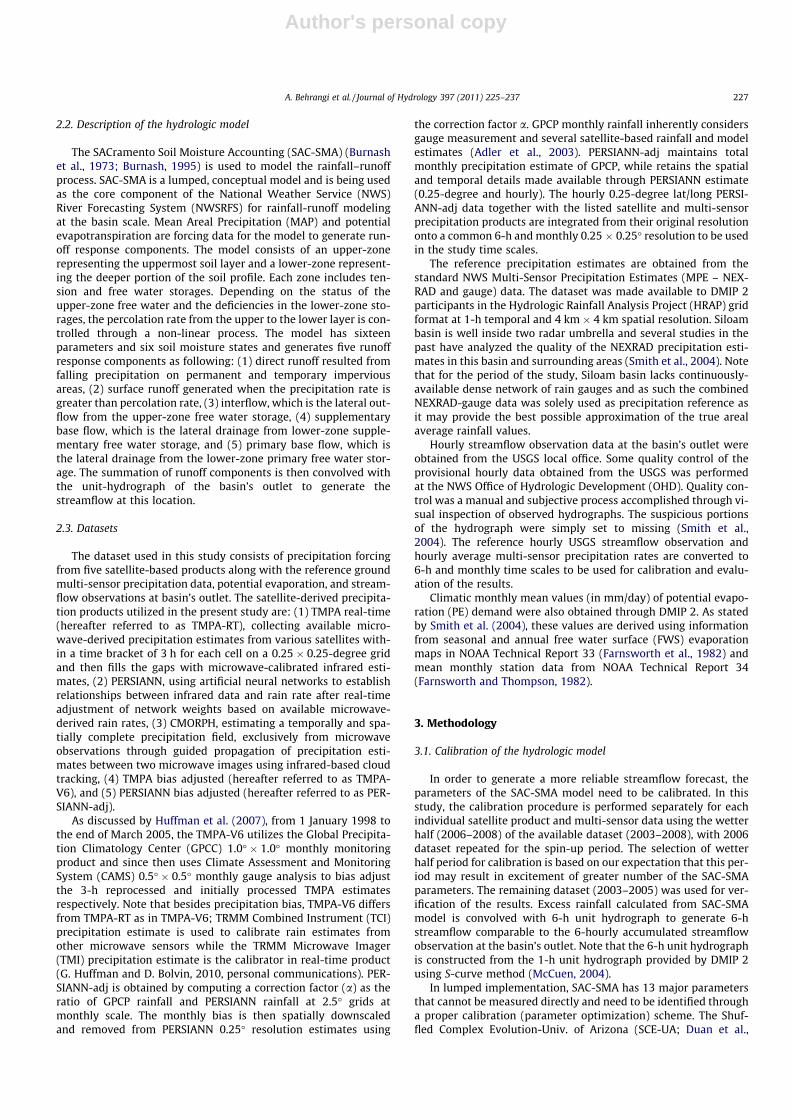
Fig. 2. Six-hour basin averaged precipitation time-series: (a) multi-sensor (reference), (b) TMPA-RT, (c) PERSIANN, (d) CMORPH, (e) TMPA-V6 and (f) PERSIANN-adj.



FAR range from 0 to 1, with perfection represented by a POD of 1and a FAR of 0. POD is sensitive to number of pixels correctly clas-sified as precipitation (Hits). FAR, on the other hand, is sensitive tonumber of pixels incorrectly classified as no-precipitation (Falsealarm). As a result, a low POD can be increased by increasing thepredicted rain coverage, but such improvement would be at thecost of increasing false alarms. A value of 1 for BIASa indicates thatpredictions and observations have identical area coverage inde-pendent of location. The ETS ranges between �1/3 and 1 with per-fection represented by ETS of 1. It allows the scores to be compared‘‘equitably’’ across different regimes (Schaefer, 1990) and is insen-sitive to systematic over- or under-estimation.

4. Results

4.1. Evaluation of precipitation forcing

Fig. 2 shows the 6-h basin averaged precipitation time-series(2003–2008) for reference multi-sensor precipitation (Fig. 2a)and other precipitation products (Fig. 2b–f). Visual inspection ofprecipitation rates and pattern in conjunction with quantitativestatistics, reported at the top-right corner of each panel, demon-strates high agreement between satellite products and thereference multi-sensor data. The satellite products with no bias-adjustment (Fig. 2b–d) agree well among themselves as quantifiedby COR, RMSE and BIAS ranging between (0.66–0.79), (0.51–0.61 mm/h), and (27.6–40.1%), respectively. The two monthlybias-adjusted satellite products (Fig. 2e and f) is very alike withsubstantial improvement compared to their near real-time coun-terparts. Fig. 2 also suggests that the satellite products with nobias-adjustment show a strong tendency to overestimate intenseprecipitation events. As expected, after bias adjustment, the over

and under-estimations are significantly reduced with overall sta-tistics demonstrating negligible BIAS for TMPA-V6 (1.7%) and PER-SIANN-adj (6.2%).

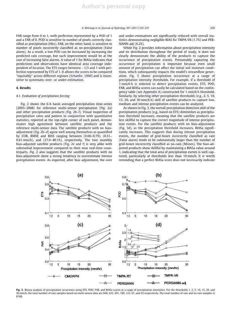
While Fig. 2 provides information about precipitation intensityand its distribution throughout the period of study, it does notclearly demonstrate the ability of the products to capture theoccurrence of precipitation events. Presumably capturing theoccurrence of precipitation is important because even smallamount of precipitation can affect the initial soil moisture condi-tions, which subsequently impacts the model’s streamflow gener-ation. Fig. 3 shows precipitation occurrence at a range ofprecipitation intensity thresholds. For example, if a threshold of1 mm/6 h is selected to detect precipitation events, ETS, POD,FAR, and BIASa scores can easily be calculated based on the contin-gency table (see Appendix A) constructed for 1 mm/6 h threshold.Similarly, by selecting other precipitation thresholds (e.g., 2, 5, 10,15, 20, and 30 mm/6 h) skill of satellite products to capture low,medium and intense precipitation events can be analyzed.

As shown in Fig. 3, the overall precipitation detection skill of theprecipitation products (e.g., based on ETS) diminishes as precipita-tion threshold increases, meaning that the satellite products areless skillful to capture the correct magnitude of intense precipita-tion events. For the satellite products with no bias-adjustment(Fig. 3d), as the precipitation threshold increases, BIASa signifi-cantly increases. This suggests that during intense precipitationevents, the number of grid-boxes incorrectly classified as rain(False alarm) tends to be substantially larger than the number ofgrid-boxes incorrectly classified as no-rain (Misses). The bias-ad-justed products show skillful by maintaining a BIASa value around1, indicating that the total area of precipitation events is well cap-tured, particularly at thresholds less than 10 mm/h. It is worthreminding that a perfect BIASa score does not necessarily indicate

Fig. 3. Binary analysis of precipitation occurrence using ETS, POD, FAR, and BIASa scores at a range of precipitation intensities. For the thresholds 1, 2, 5, 10, 15, 20, and30 mm/h, the total number of rain samples based on multi-sensor data are 846, 635, 391, 188, 123, 67, and 24 respectively. The total number of rain and no-rain samples is8768.



a perfect match between precipitation/no-precipitation grid-boxesof observed and predicted fields. CMORPH demonstrates high skillsin detecting precipitation events across the entire range of precip-itation intensities (see Fig. 3b). However, similar to TMPA-RT, itsignificantly overestimates the intense precipitation areas(Fig. 3d). From Fig. 3 and based on ETS, CMORPH outperforms allsatellite products, including those that are bias-adjusted, in delin-eation of precipitation areas within an intensity range of less than15 mm/6 h. As discussed by Behrangi et al. (2009) and Behrangiet al. (2010a), one reason for this could be due to inability of infra-red based precipitation estimation algorithms (e.g., PERSIANN andpartially TMPA) to: (a) capture warm rainfall and (b) screen out no-rain thin cirrus clouds that are usually very cold. The first short-coming may result in significant under-estimation of the total vol-ume of rainfall, while the latter may result in assigningprecipitation to areas with no-precipitation.

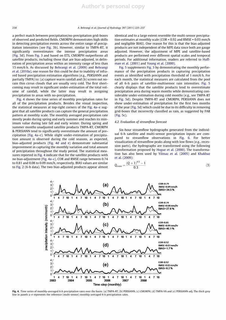
Fig. 4 shows the time series of monthly precipitation rates forall of the precipitation products. Besides the visual inspection,the statistical measures at top-right corners of the Fig. 4a–e sug-gest that all satellite products can capture the general precipitationpattern at monthly scale. The monthly averaged precipitation ratemostly peaks during spring and early summer and reaches its min-imum value during late fall and early winter. During spring andsummer months unadjusted satellite products TMPA-RT, CMORPH& PERSIANN tend to significantly overestimate the amount of pre-cipitation (Fig. 4a–c). While slight under-estimation of precipita-tion amount is observed during the cold seasons, as expected,bias-adjusted products (Fig. 4d and e) demonstrate substantialimprovement in capturing the monthly variation and total amountof precipitation throughout the study period. The statistical mea-sures reported in Fig. 4 indicate that for the satellite products withno bias-adjustment (Fig. 4a–c), COR and RMSE range between 0.74to 0.81 and 0.08 to 0.09 mm/h, respectively. BIAS values are similarto Fig. 2 (6-h data). The two bias-adjusted products appear almost

identical and to a large extent resemble the multi-sensor precipita-tion estimates at monthly scale (COR = 0.92 and RMSE = 0.03 mm/hand negligible BIAS). One reason for this is that the bias-adjustedproducts are not independent of the MPE data since both are gaugeadjusted. However, the adjustment of MPE and satellite-basedproducts are performed over different spatial scales and temporalperiods. For additional information, readers are referred to Huff-man et al. (2001) and Young et al. (2000).

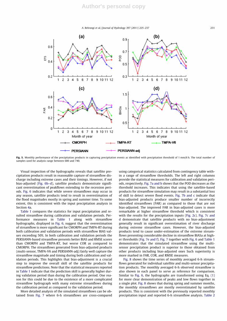
Fig. 5 supplements Fig. 3 by demonstrating the monthly perfor-mance of the precipitation products in capturing precipitationevents as identified with precipitation threshold of 1 mm/6 h. Foreach month, the statistical measures are calculated from the poolof all 6-h pairs of satellite-multisensor rain intensities. Fig. 5clearly displays that the satellite products tend to overestimateprecipitation area during warm months while demonstrating con-siderable under-estimation during cold months (e.g., see TMPA-RTin Fig. 5d). Despite TMPA-RT and CMORPH, PERSIANN does notshow under-estimation of precipitation for the first two monthsof the year (Fig. 5d) which could be due to its difficulty in removinggrid-boxes that incorrectly classified as rain, as suggested by FAR(Fig. 5c).

4.2. Evaluation of streamflow forecast

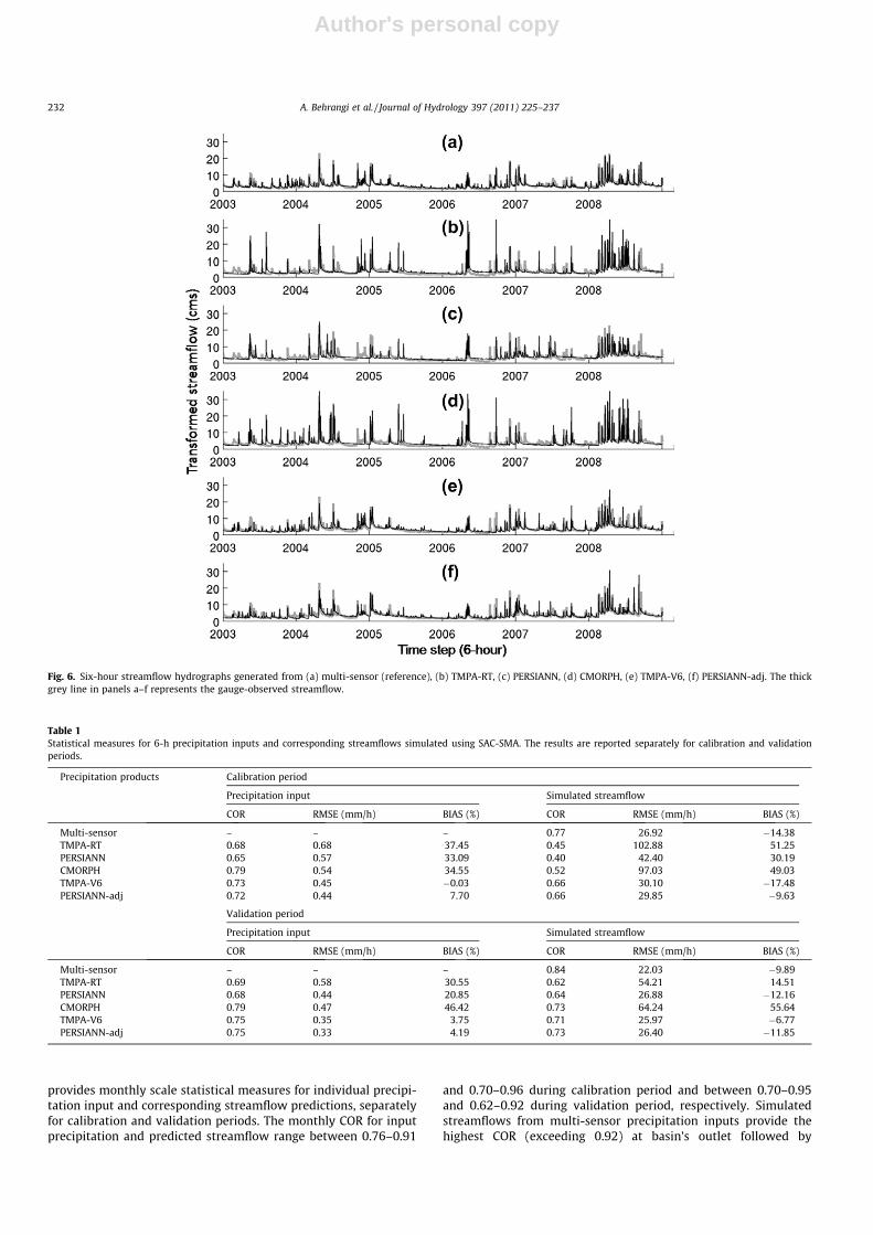
Six-hour streamflow hydrographs generated from the individ-ual 6-h satellite and multi-sensor precipitation inputs are com-pared to streamflow observations in Fig. 6. For bettervisualization of streamflow peaks along with low flows (e.g., reces-sion parts), the hydrographs are transformed using the followingtransformation proposed by Hogue et al. (2000). The transforma-tion has also been used by Yilmaz et al. (2005) and Khakbazet al. (2009):

Qtrans ¼ðQ þ 1Þ0:3 � 1

0:3ð3Þ

Fig. 4. Time series of monthly-averaged 6-h precipitation rates over the basin: (a) TMPA-RT, (b) PERSIANN, (c) CMORPH, (d) TMPA-V6 and (e) PERSIANN-adj. The thick greyline in panels a–e represents the reference (multi-sensor) monthly-averaged 6-h precipitation rates.



Visual inspection of the hydrographs reveals that satellite pre-cipitation products result in reasonable capture of streamflow dis-charge including extreme cases and their timings. However, if notbias-adjusted (Fig. 6b–d), satellite products demonstrate signifi-cant overestimation of peakflows extending to the recession peri-ods. Fig. 6 indicates that while severe streamflows may occur inany season, satellite products tend to result in overestimation ofthe flood magnitudes mostly in spring and summer time. To someextent, this is consistent with the input precipitation analysis inSection 4a.

Table 1 compares the statistics for input precipitation and re-sulted streamflow during calibration and validation periods. Per-formance measures in Table 1 along with streamflowhydrographs, displayed in Fig. 6, suggest that the overestimationof streamflow is more significant for CMORPH and TMPA-RT duringboth calibration and validation periods with streamflow BIAS val-ues exceeding 50%. In both calibration and validation periods thePERSIANN-based streamflow presents better BIAS and RMSE scoresthan CMORPH and TMPA-RT, but worse COR as compared toCMORPH. The streamflows generated from bias-adjusted products(multi-sensor, TMPA-V6 and PERSIANN-adj) fairly well capture thestreamflow magnitude and timing during both calibration and val-idation periods. This highlights that bias-adjustment is a crucialstep to improve the overall skill of the satellite products forstreamflow predictions. Note that the statistical measures reportedin Table 1 indicate that the prediction skill is generally higher dur-ing validation period than during the calibration period. One rea-son for this could be due to the existence of a more complicatedstreamflow hydrograph with many extreme streamflows duringthe calibration period as compared to the validation period.

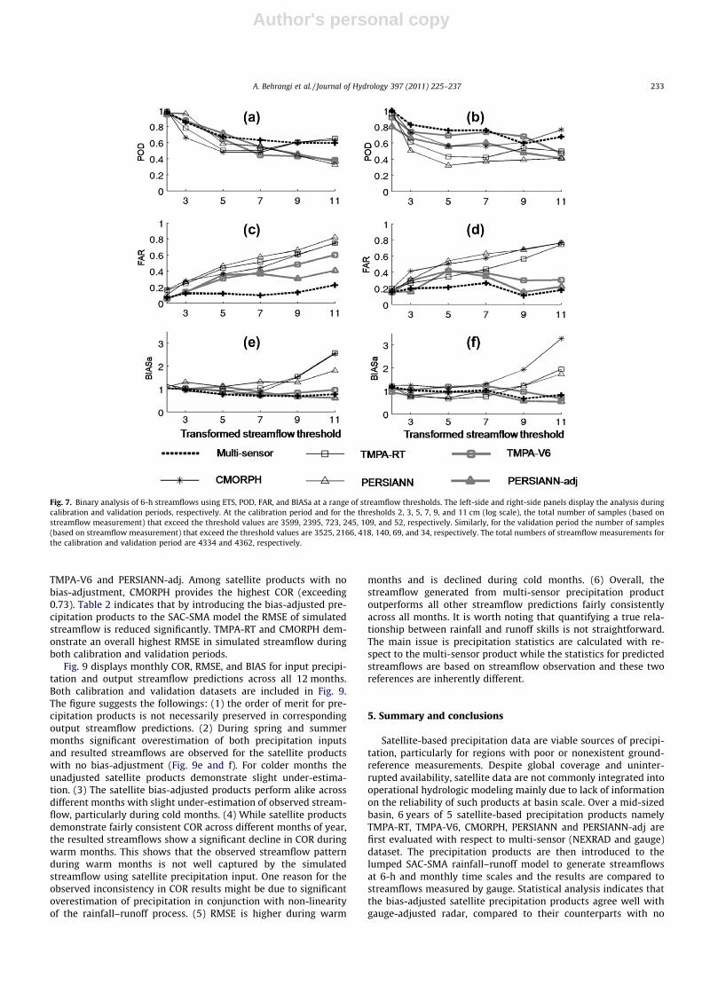
More detailed analysis of the simulated streamflows can be ob-tained from Fig. 7 where 6-h streamflows are cross-compared

using categorical statistics calculated from contingency table with-in a range of streamflow thresholds. The left and right columnsprovide the statistical measures for calibration and validation peri-ods, respectively. Fig. 7a and b shows that the POD decreases as thethreshold increases. This indicates that using the satellite-basedproducts for streamflow simulation may result in a substantial lossof skill to detect severe flood events. Fig. 7b and c indicate thatbias-adjusted products produce smaller number of incorrectlyidentified streamflows (FAR) as compared to those that are notbias-adjusted. The improved FAR in bias-adjusted cases is moreremarkable at higher streamflow threshold which is consistentwith the results for the precipitation inputs (Fig. 2c). Fig. 7c andd demonstrate that satellite products with no bias-adjustmentgenerally result in significant overestimation of river dischargeduring extreme streamflow cases. However, the bias-adjustedproducts tend to cause under-estimation of the extreme stream-flows presenting considerable decline in streamflow BIASa at high-er thresholds (Fig. 7e and f). Fig. 7 together with Fig. 6 and Table 1demonstrates that the simulated streamflow using the multi-sensor precipitation product is superior to those obtained fromother products including bias-adjusted ones Such superiority ismore marked in FAR, COR, and RMSE measures.

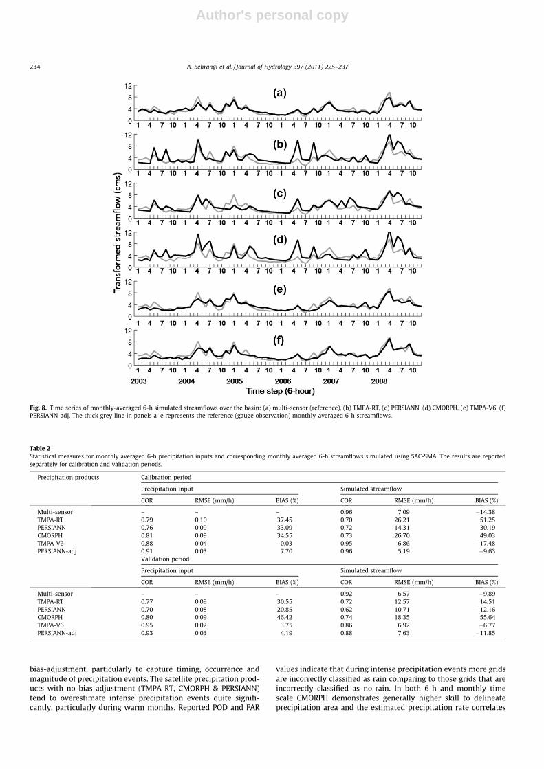
Fig. 8 shows the time series of monthly averaged 6-h stream-flows generated for individual satellite and multi-sensor precipita-tion products. The monthly averaged 6-h observed streamflow isalso shown in each panel to serve as reference for comparison.Similar to Fig. 6, the hydrographs are transformed using Eq. (1)for more clear demonstration of peaks and low flows together ina single plot. Fig. 8 shows that during spring and summer months,the monthly streamflows are mostly overestimated by satelliteproducts. This is consistent with the previously reported monthlyprecipitation input and reported 6-h streamflow analysis. Table 2

Fig. 5. Monthly performance of the precipitation products in capturing precipitation events as identified with precipitation threshold of 1 mm/6 h. The total number ofsamples used for analysis range between 680 and 740.



provides monthly scale statistical measures for individual precipi-tation input and corresponding streamflow predictions, separatelyfor calibration and validation periods. The monthly COR for inputprecipitation and predicted streamflow range between 0.76–0.91

and 0.70–0.96 during calibration period and between 0.70–0.95and 0.62–0.92 during validation period, respectively. Simulatedstreamflows from multi-sensor precipitation inputs provide thehighest COR (exceeding 0.92) at basin’s outlet followed by

Fig. 6. Six-hour streamflow hydrographs generated from (a) multi-sensor (reference), (b) TMPA-RT, (c) PERSIANN, (d) CMORPH, (e) TMPA-V6, (f) PERSIANN-adj. The thickgrey line in panels a–f represents the gauge-observed streamflow.

Table 1Statistical measures for 6-h precipitation inputs and corresponding streamflows simulated using SAC-SMA. The results are reported separately for calibration and validationperiods.

Precipitation products Calibration period

Precipitation input Simulated streamflow

COR RMSE (mm/h) BIAS (%) COR RMSE (mm/h) BIAS (%)

Multi-sensor – – – 0.77 26.92 �14.38TMPA-RT 0.68 0.68 37.45 0.45 102.88 51.25PERSIANN 0.65 0.57 33.09 0.40 42.40 30.19CMORPH 0.79 0.54 34.55 0.52 97.03 49.03TMPA-V6 0.73 0.45 �0.03 0.66 30.10 �17.48PERSIANN-adj 0.72 0.44 7.70 0.66 29.85 �9.63

Validation period



Multi-sensor – – – 0.84 22.03 �9.89TMPA-RT 0.69 0.58 30.55 0.62 54.21 14.51PERSIANN 0.68 0.44 20.85 0.64 26.88 �12.16CMORPH 0.79 0.47 46.42 0.73 64.24 55.64TMPA-V6 0.75 0.35 3.75 0.71 25.97 �6.77PERSIANN-adj 0.75 0.33 4.19 0.73 26.40 �11.85



TMPA-V6 and PERSIANN-adj. Among satellite products with nobias-adjustment, CMORPH provides the highest COR (exceeding0.73). Table 2 indicates that by introducing the bias-adjusted pre-cipitation products to the SAC-SMA model the RMSE of simulatedstreamflow is reduced significantly. TMPA-RT and CMORPH dem-onstrate an overall highest RMSE in simulated streamflow duringboth calibration and validation periods.

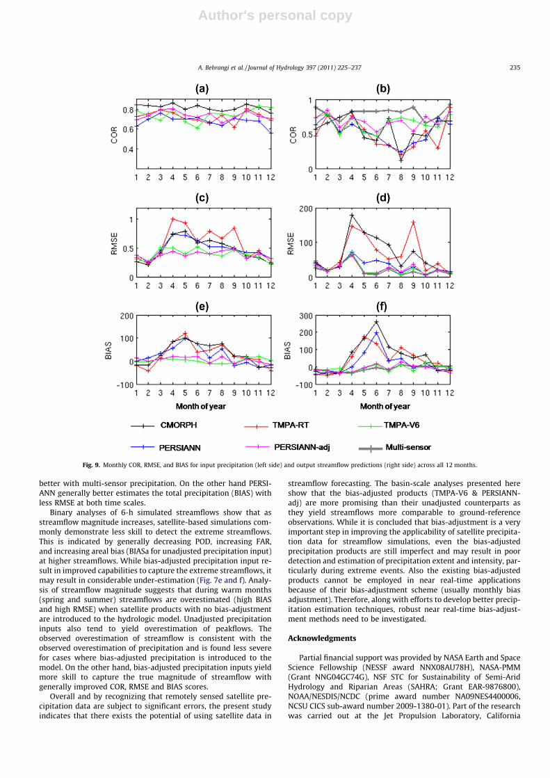
Fig. 9 displays monthly COR, RMSE, and BIAS for input precipi-tation and output streamflow predictions across all 12 months.Both calibration and validation datasets are included in Fig. 9.The figure suggests the followings: (1) the order of merit for pre-cipitation products is not necessarily preserved in correspondingoutput streamflow predictions. (2) During spring and summermonths significant overestimation of both precipitation inputsand resulted streamflows are observed for the satellite productswith no bias-adjustment (Fig. 9e and f). For colder months theunadjusted satellite products demonstrate slight under-estima-tion. (3) The satellite bias-adjusted products perform alike acrossdifferent months with slight under-estimation of observed stream-flow, particularly during cold months. (4) While satellite productsdemonstrate fairly consistent COR across different months of year,the resulted streamflows show a significant decline in COR duringwarm months. This shows that the observed streamflow patternduring warm months is not well captured by the simulatedstreamflow using satellite precipitation input. One reason for theobserved inconsistency in COR results might be due to significantoverestimation of precipitation in conjunction with non-linearityof the rainfall–runoff process. (5) RMSE is higher during warm

months and is declined during cold months. (6) Overall, thestreamflow generated from multi-sensor precipitation productoutperforms all other streamflow predictions fairly consistentlyacross all months. It is worth noting that quantifying a true rela-tionship between rainfall and runoff skills is not straightforward.The main issue is precipitation statistics are calculated with re-spect to the multi-sensor product while the statistics for predictedstreamflows are based on streamflow observation and these tworeferences are inherently different.

5. Summary and conclusions

Satellite-based precipitation data are viable sources of precipi-tation, particularly for regions with poor or nonexistent ground-reference measurements. Despite global coverage and uninter-rupted availability, satellite data are not commonly integrated intooperational hydrologic modeling mainly due to lack of informationon the reliability of such products at basin scale. Over a mid-sizedbasin, 6 years of 5 satellite-based precipitation products namelyTMPA-RT, TMPA-V6, CMORPH, PERSIANN and PERSIANN-adj arefirst evaluated with respect to multi-sensor (NEXRAD and gauge)dataset. The precipitation products are then introduced to thelumped SAC-SMA rainfall–runoff model to generate streamflowsat 6-h and monthly time scales and the results are compared tostreamflows measured by gauge. Statistical analysis indicates thatthe bias-adjusted satellite precipitation products agree well withgauge-adjusted radar, compared to their counterparts with no

Fig. 7. Binary analysis of 6-h streamflows using ETS, POD, FAR, and BIASa at a range of streamflow thresholds. The left-side and right-side panels display the analysis duringcalibration and validation periods, respectively. At the calibration period and for the thresholds 2, 3, 5, 7, 9, and 11 cm (log scale), the total number of samples (based onstreamflow measurement) that exceed the threshold values are 3599, 2395, 723, 245, 109, and 52, respectively. Similarly, for the validation period the number of samples(based on streamflow measurement) that exceed the threshold values are 3525, 2166, 418, 140, 69, and 34, respectively. The total numbers of streamflow measurements forthe calibration and validation period are 4334 and 4362, respectively.



bias-adjustment, particularly to capture timing, occurrence andmagnitude of precipitation events. The satellite precipitation prod-ucts with no bias-adjustment (TMPA-RT, CMORPH & PERSIANN)tend to overestimate intense precipitation events quite signifi-cantly, particularly during warm months. Reported POD and FAR

values indicate that during intense precipitation events more gridsare incorrectly classified as rain comparing to those grids that areincorrectly classified as no-rain. In both 6-h and monthly timescale CMORPH demonstrates generally higher skill to delineateprecipitation area and the estimated precipitation rate correlates

Fig. 8. Time series of monthly-averaged 6-h simulated streamflows over the basin: (a) multi-sensor (reference), (b) TMPA-RT, (c) PERSIANN, (d) CMORPH, (e) TMPA-V6, (f)PERSIANN-adj. The thick grey line in panels a–e represents the reference (gauge observation) monthly-averaged 6-h streamflows.

Table 2Statistical measures for monthly averaged 6-h precipitation inputs and corresponding monthly averaged 6-h streamflows simulated using SAC-SMA. The results are reportedseparately for calibration and validation periods.

Precipitation products Calibration period



Multi-sensor – – – 0.96 7.09 �14.38TMPA-RT 0.79 0.10 37.45 0.70 26.21 51.25PERSIANN 0.76 0.09 33.09 0.72 14.31 30.19CMORPH 0.81 0.09 34.55 0.73 26.70 49.03TMPA-V6 0.88 0.04 �0.03 0.95 6.86 �17.48PERSIANN-adj 0.91 0.03 7.70 0.96 5.19 �9.63

Validation period



Multi-sensor – – – 0.92 6.57 �9.89TMPA-RT 0.77 0.09 30.55 0.72 12.57 14.51PERSIANN 0.70 0.08 20.85 0.62 10.71 �12.16CMORPH 0.80 0.09 46.42 0.74 18.35 55.64TMPA-V6 0.95 0.02 3.75 0.86 6.92 �6.77PERSIANN-adj 0.93 0.03 4.19 0.88 7.63 �11.85



better with multi-sensor precipitation. On the other hand PERSI-ANN generally better estimates the total precipitation (BIAS) withless RMSE at both time scales.

Binary analyses of 6-h simulated streamflows show that asstreamflow magnitude increases, satellite-based simulations com-monly demonstrate less skill to detect the extreme streamflows.This is indicated by generally decreasing POD, increasing FAR,and increasing areal bias (BIASa for unadjusted precipitation input)at higher streamflows. While bias-adjusted precipitation input re-sult in improved capabilities to capture the extreme streamflows, itmay result in considerable under-estimation (Fig. 7e and f). Analy-sis of streamflow magnitude suggests that during warm months(spring and summer) streamflows are overestimated (high BIASand high RMSE) when satellite products with no bias-adjustmentare introduced to the hydrologic model. Unadjusted precipitationinputs also tend to yield overestimation of peakflows. Theobserved overestimation of streamflow is consistent with theobserved overestimation of precipitation and is found less severefor cases where bias-adjusted precipitation is introduced to themodel. On the other hand, bias-adjusted precipitation inputs yieldmore skill to capture the true magnitude of streamflow withgenerally improved COR, RMSE and BIAS scores.

Overall and by recognizing that remotely sensed satellite pre-cipitation data are subject to significant errors, the present studyindicates that there exists the potential of using satellite data in

streamflow forecasting. The basin-scale analyses presented hereshow that the bias-adjusted products (TMPA-V6 & PERSIANN-adj) are more promising than their unadjusted counterparts asthey yield streamflows more comparable to ground-referenceobservations. While it is concluded that bias-adjustment is a veryimportant step in improving the applicability of satellite precipita-tion data for streamflow simulations, even the bias-adjustedprecipitation products are still imperfect and may result in poordetection and estimation of precipitation extent and intensity, par-ticularly during extreme events. Also the existing bias-adjustedproducts cannot be employed in near real-time applicationsbecause of their bias-adjustment scheme (usually monthly biasadjustment). Therefore, along with efforts to develop better precip-itation estimation techniques, robust near real-time bias-adjust-ment methods need to be investigated.

Acknowledgments

Partial financial support was provided by NASA Earth and SpaceScience Fellowship (NESSF award NNX08AU78H), NASA-PMM(Grant NNG04GC74G), NSF STC for Sustainability of Semi-AridHydrology and Riparian Areas (SAHRA; Grant EAR-9876800),NOAA/NESDIS/NCDC (prime award number NA09NES4400006,NCSU CICS sub-award number 2009-1380-01). Part of the researchwas carried out at the Jet Propulsion Laboratory, California

Fig. 9. Monthly COR, RMSE, and BIAS for input precipitation (left side) and output streamflow predictions (right side) across all 12 months.



Institute of Technology, under a contract with the NationalAeronautics and Space Administration.

Appendix A:. Definition of the statistical measures used in thisstudy

(a) Quantitative statistics, which are obtained using estimatedand observed quantities. For example, if PRest and PRobs rep-resent estimated and observed precipitation rates, the quan-titative statistics used in the present work are defined asbelow:

Correlation coefficient ðCORÞ

¼PN

i¼1 PRobsð ÞiðPRestÞi� �

� NðPRobsÞPRestÞ� �

ffiffiffiffiffiffiffiffiffiffiffiffiffiffiffiffiffiffiffiffiffiffiffiffiffiffiffiffiffiffiffiffiffiffiffiffiffiffiffiffiffiffiffiffiffiffiffiffiffiffiffiffiffiffiffiffiffiffiffiffiffiffiffiffiffiffiffiffiffiffiffiffiffiffiffiffiffiffiffiffiffiffiffiffiffiffiffiffiffiffiffiffiffiffiffiffiffiffiffiffiffiffiffiffiffiffiffiffiffiffiffiffiPNi¼1ðPRobsÞ2i � NðPRobsÞ2

h i PNi¼1ðPRestÞ2i � NðPRestÞ2

h ir

Root mean square ðRMSEÞ

¼ 1N

XN

i¼1ðPRestðiÞ � PRobsðiÞÞ2

0:5

Percent bias ðBIASÞ ¼PN

i¼1 RRestðiÞ � RRobsðiÞð ÞN

� 100

where N is the total number of observed and estimated rainpairs.

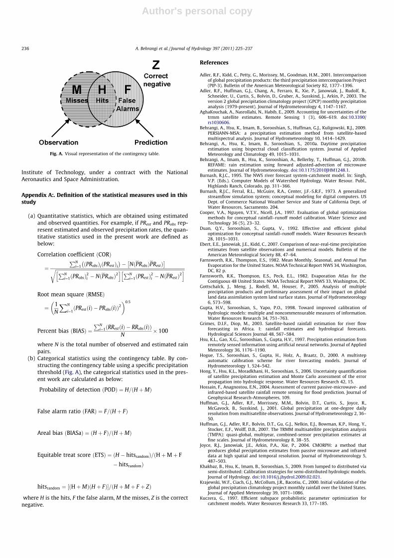
(b) Categorical statistics using the contingency table. By con-structing the contingency table using a specific precipitationthreshold (Fig. A), the categorical statistics used in the pres-ent work are calculated as below:

Probability of detection ðPODÞ ¼ H=ðH þMÞ

False alarm ratio ðFARÞ ¼ F=ðH þ FÞ

Areal bias ðBIASaÞ ¼ ðH þ FÞ=ðH þMÞ

Equitable treat score ðETSÞ ¼ ðH � hitsrandomÞ=ðHþMþ F

� hitsrandomÞ

hitsrandom ¼ ðHþMÞðH þ FÞ½ �=ðH þM þ F þ ZÞ

where H is the hits, F the false alarm, M the misses, Z is the correctnegative.

References

Adler, R.F., Kidd, C., Petty, G., Morissey, M., Goodman, H.M., 2001. Intercomparisonof global precipitation products: the third precipitation intercomparison Project(PIP-3). Bulletin of the American Meteorological Society 82, 1377–1396.

Adler, R.F., Huffman, G.J., Chang, A., Ferraro, R., Xie, P., Janowiak, J., Rudolf, B.,Schneider, U., Curtis, S., Bolvin, D., Gruber, A., Susskind, J., Arkin, P., 2003. Theversion 2 global precipitation climatology project (GPCP) monthly precipitationanalysis (1979-present). Journal of Hydrometeorology 4, 1147–1167.

AghaKouchak, A., Nasrollahi, N., Habib, E., 2009. Accounting for uncertainties of thetrmm satellite estimates. Remote Sensing 1 (3), 606–619. doi:10.3390/rs1030606.

Behrangi, A., Hsu, K., Imam, B., Sorooshian, S., Huffman, G.J., Kuligowski, R.J., 2009.PERSIANN-MSA: a precipitation estimation method from satellite-basedmultispectral analysis. Journal of Hydrometeorology 10, 1414–1429.

Behrangi, A., Hsu, K., Imam, B., Sorooshian, S., 2010a. Daytime precipitationestimation using bispectral cloud classification system. Journal of AppliedMeteorology and Climatology 49, 1015–1031.

Behrangi, A., Imam, B., Hsu, K., Sorooshian, A., Bellerby, T., Huffman, G.J., 2010b.REFAME: rain estimation using forward adjusted-advection of microwaveestimates. Journal of Hydrometeorology. doi:10.1175/2010JHM1248.1.

Burnash, R.J.C., 1995. The NWS river forecast system-catchment model. In: Singh,V.P. (Eds.). Computer Models of Watershed Hydrology. Water Resour. Publ.,Highlands Ranch, Colorado, pp. 311–366.

Burnash, R.J.C., Ferral, R.L., McGuire, R.A., Center, J.F.-S.R.F., 1973. A generalizedstreamflow simulation system; conceptual modeling for digital computers. USDept. of Commerce National Weather Service and State of California Dept. ofWater Resources, Sacramento. 204.

Cooper, V.A., Nguyen, V.T.V., Nicell, J.A., 1997. Evaluation of global optimizationmethods for conceptual rainfall–runoff model calibration. Water Science andTechnology 36 (5), 23–32.

Duan, Q.Y., Sorooshian, S., Gupta, V., 1992. Effective and efficient globaloptimization for conceptual rainfall–runoff models. Water Resources Research28, 1015–1031.

Ebert, E.E., Janowiak, J.E., Kidd, C., 2007. Comparison of near-real-time precipitationestimates from satellite observations and numerical models. Bulletin of theAmerican Meteorological Society 88, 47–64.

Farnsworth, R.K., Thompson, E.S., 1982. Mean Monthly, Seasonal, and Annual PanEvaporation for the United States. NOAA Technical Report NWS 34, Washington,DC, 82 p.

Farnsworth, R.K., Thompson, E.S., Peck, E.L., 1982. Evaporation Atlas for theContiguous 48 United States. NOAA Technical Report NWS 33, Washington, DC.

Gottschalck, J., Meng, J., Rodell, M., Houser, P., 2005. Analysis of multipleprecipitation products and preliminary assessment of their impact on globalland data assimilation system land surface states. Journal of Hydrometeorology6, 573–598.

Gupta, H.V., Sorooshian, S., Yapo, P.O., 1998. Toward improved calibration ofhydrologic models: multiple and noncommensurable measures of information.Water Resources Research 34, 751–763.

Grimes, D.I.F., Diop, M., 2003. Satellite-based rainfall estimation for river flowforecasting in Africa. I: rainfall estimates and hydrological forecasts.Hydrological Sciences Journal 48, 567–584.

Hsu, K.L., Gao, X.G., Sorooshian, S., Gupta, H.V., 1997. Precipitation estimation fromremotely sensed information using artificial neural networks. Journal of AppliedMeteorology 36, 1176–1190.

Hogue, T.S., Sorooshian, S., Gupta, H., Holz, A., Braatz, D., 2000. A multistepautomatic calibration scheme for river forecasting models. Journal ofHydrometeorology 1, 524–542.

Hong, Y., Hsu, K.L., Moradkhani, H., Sorooshian, S., 2006. Uncertainty quantificationof satellite precipitation estimation and Monte Carlo assessment of the errorpropagation into hydrologic response. Water Resources Research 42, 15.

Hossain, F., Anagnostou, E.N., 2004. Assessment of current passive-microwave- andinfrared-based satellite rainfall remote sensing for flood prediction. Journal ofGeophysical Research-Atmospheres, 109.

Huffman, G.J., Adler, R.F., Morrissey, M.M., Bolvin, D.T., Curtis, S., Joyce, R.,McGavock, B., Susskind, J., 2001. Global precipitation at one-degree dailyresolution from multisatellite observations. Journal of Hydrometeorology 2, 36–50.

Huffman, G.J., Adler, R.F., Bolvin, D.T., Gu, G.J., Nelkin, E.J., Bowman, K.P., Hong, Y.,Stocker, E.F., Wolff, D.B., 2007. The TRMM multisatellite precipitation analysis(TMPA): quasi-global, multiyear, combined-sensor precipitation estimates atfine scales. Journal of Hydrometeorology 8, 38–55.

Joyce, R.J., Janowiak, J.E., Arkin, P.A., Xie, P., 2004. CMORPH: a method thatproduces global precipitation estimates from passive microwave and infrareddata at high spatial and temporal resolution. Journal of Hydrometeorology 5,487–503.

Khakbaz, B., Hsu, K., Imam, B., Sorooshian, S., 2009. From lumped to distributed viasemi-distributed: Calibration strategies for semi-distributed hydrologic models.Journal of Hydrology. doi:10.1016/j.jhydrol.2009.02.021.

Krajewski, W.F., Ciach, G.J., McCollum, J.R., Bacotiu, C., 2000. Initial validation of theglobal precipitation climatology project monthly rainfall over the United States.Journal of Applied Meteorology 39, 1071–1086.

Kuczera, G., 1997. Efficient subspace probabilistic parameter optimization forcatchment models. Water Resources Research 33, 177–185.

Fig. A. Visual representation of the contingency table.



McCollum, J.R., Krajewski, W.F., Ferraro, R.R., Ba, M.B., 2002. Evaluation of biases ofsatellite rainfall estimation algorithms over the continental United States.Journal of Applied Meteorology 41, 1065–1080.

McCuen, R.H., 2004. Hydrologic Analysis and Design. Prentice Hall, 888 pp.Nelder, J.A., Mead, R., 1965. A simplex-method for function minimization. Computer

Journal 7 (4), 308–313.Nijssen, B., Lettenmaier, D.P., 2004. Effect of precipitation sampling error on

simulated hydrological fluxes and states: anticipating the global precipitationmeasurement satellites. Journal of Geophysical Research 109, D02103.

Schaefer, J.T., 1990. The critical success index as an indicator of warning Skill.Weather and Forecasting 5, 570–575.

Schultz, G.A., 1996. Remote sensing applications to hydrology: runoff. HydrologicalSciences Journal 41, 453–475.

Stokstad, E., 1999. Scarcity of rain, stream gages threatens forecasts. Science 285,1199–1200.

Shiklomanov, A.I., Lammers, R.B., Vörösmarty, C.J., 2002. Widespread decline inhydrological monitoring threatens pan-Arctic research. Eos, TransactionsAmerican Geophysical Union 83, 13.

Smith, M.B., Seo, D.J., Koren, V.I., Reed, S.M., Zhang, Z., Duan, Q., Moreda, F., Cong, S.,2004. The distributed model intercomparison project (DMIP): motivation andexperiment design. Journal of Hydrology 298, 4–26.

Sorooshian, S., Hsu, K.L., Gao, X., Gupta, H.V., Imam, B., Braithwaite, D., 2000.Evaluation of PERSIANN system satellite-based estimates of tropical rainfall.Bulletin of the American Meteorology Society 81, 2035–2046.

Su, F., Hong, Y., Lettenmaier, D.P., 2008. Evaluation of TRMM multisatelliteprecipitation analysis (TMPA) and its utility in hydrologic prediction in the LaPlata basin. Journal of Hydrometeorology 9, 622–640.

Tsintikidis, D., Georgakakos, K.P., Artan, G.A., Tsonis, A.A., 1999. A feasibility studyon mean areal rainfall estimation and hydrologic response in the Blue Nileregion using METEOSAT images. Journal of Hydrology 221, 97–116.

Turk, F.J., Rohaly, G.D., Hawkins, J., Smith, E.A., Marzano, F.S., Mugnai, A., Levizzani,V., 2000. Meteorological applications of precipitation estimation fromcombined SSM/I, TRMM and infrared geostationary satellite data. In:Pampaloni, P., Paloscia, S. (Eds.). Microwave Radiometry and Remote Sensingof the Earth’s Surface and Atmosphere. VSP Int. Sci. Publ., pp. 353–363.

Thyer, M., Kuczera, G., Bates, B.C., 1999. Probabilistic optimization for conceptualrainfall–runoff models: a comparison of the shuffled complex evolution andsimulated annealing algorithms. Water Resources Research 35, 767–773.

Yilmaz, K.K., Hogue, T.S., Hsu, K.L., Sorooshian, S., Gupta, H.V., Wagener, T., 2005.Intercomparison of rain gauge, radar, and satellite-based precipitationestimates with emphasis on hydrologic forecasting. Journal ofHydrometeorology 6, 497–517.

Young, C.B., Bradley, A.A., Krajewski, W.F., Kruger, A., 2000. Evaluating NEXRADmultisensor precipitation estimates for operational hydrologic forecasting.Journal of Hydrometeorology 1, 241–254.


Author's personal copy - Amir...

Documents

Transcript of Author's personal copy - Amir...