The Analysis of Random Polling SystemsAuthor(s): Leonard Kleinrock and Hanoch LevySource: Operations Research, Vol. 36, No. 5 (Sep. - Oct., 1988), pp. 716-732Published by: INFORMSStable URL: http://www.jstor.org/stable/171317Accessed: 17/11/2009 16:46

Your use of the JSTOR archive indicates your acceptance of JSTOR's Terms and Conditions of Use, available athttp://www.jstor.org/page/info/about/policies/terms.jsp. JSTOR's Terms and Conditions of Use provides, in part, that unlessyou have obtained prior permission, you may not download an entire issue of a journal or multiple copies of articles, and youmay use content in the JSTOR archive only for your personal, non-commercial use.

Please contact the publisher regarding any further use of this work. Publisher contact information may be obtained athttp://www.jstor.org/action/showPublisher?publisherCode=informs.

Each copy of any part of a JSTOR transmission must contain the same copyright notice that appears on the screen or printedpage of such transmission.

JSTOR is a not-for-profit service that helps scholars, researchers, and students discover, use, and build upon a wide range ofcontent in a trusted digital archive. We use information technology and tools to increase productivity and facilitate new formsof scholarship. For more information about JSTOR, please contact support@jstor.org.

INFORMS is collaborating with JSTOR to digitize, preserve and extend access to Operations Research.

http://www.jstor.org

THE ANALYSIS OF RANDOM POLLING SYSTEMS

LEONARD KLEINROCK University of California, Los Angeles, California

HANOCH LEVY AT&T Bell Laboratories, Holmdel, New Jersey

(Received August 1985; revisions received June 1986, February 1987; accepted September 1987)

In this paper, we analyze the behavior of random polling systems. The polling systems we consider consist of N stations, each equipped with an infinite buffer and a single server who serves them in some order. In contrast to previously studied polling systems, where the order of service used by the server is periodic (and usually cyclic), in the systems we consider the next station to be served after station i is determined by probabilistic means. More specifically, according to the model we consider in this paper, after serving station i, the server will poll (i.e., serve) station j (j = 1, 2, . . , N) with probability pj. The main results of this paper are expressions for the expected response time in a random polling system operated under a variety of service disciplines. The results are compared to the response time in the equivalent cyclic polling systems. Also in this paper, we analyze the cycle time and the number of customers found in the system.

T he queueing behavior of polling systems has been extensively investigated in the past. The "tradi-

tional" polling scheme that appears in the literature is a method by which a single server serves N stations: each generates its own stream of work requests (or customers) and each is equipped with an infinite queue to store its requests. According to this scheme, the N stations are served in a cyclic order in which the station served after station i is station i + 1 (modulo N); this is called the cyclic polling scheme.

In contrast to previous studies that dealt with (periodic and) cyclic polling schemes, our aim in this paper is to study the random polling scheme, where the polling order is not fixed. Rather, the next station polled is determined according to some random (memoryless) criterion. According to the specific scheme we investigate, the next station polled will be station j (j = 1, 2, . .. , N) with probability pj.

The traditional cyclic polling schemes have been successfully used to model systems where a central controller polls and serves many stations. A typical example is a time shared system where a single com- puter serves many terminals. In contrast, our work has been motivated by the wish to model distributed systems. In many of these distributed systems the control moves from one station to another according to some random criterion. As an example, consider a shared broadcast channel where the decision regarding "who will transmit next" is made in a distributed manner, and is based on some randomly behaving

algorithms, rather than on a fixed order. The random schemes analyzed in this paper are believed to be a natural model for such distributed systems. As an example, the results reported in this paper were used in Levy (1984) to predict the expected delay in a Slotted ALOHA system.

The main objective of this paper is to analyze the response time (waiting time plus service time) observed in the random polling systems. Specifically, the ran- dom polling scheme is studied for three types of service policy: 1) exhaustive service, 2) gated service, and 3) limited service. In the exhaustive policy, when queue i is selected for service, the server will continue to serve this queue until the queue becomes empty. Thus, all customers found in the queue at the begin- ning of the service period, and those who arrive during the service period, are served in that period. In the gated policy when queue i is selected for service, the server will serve in that service period, all (and only) those customers found in queue i at the beginning of the service period. Thus, none of the customers arriv- ing during the service period will be served during this period. In the limited service policy, the server will serve in a given service period exactly one customer (given that at least one customer is present at the polled station at the polling instant). The model is a discrete time model and the extension of the results to a continuous time model can be done in a similar way. As in the analysis of many cyclic polling systems, we allow the server to have a random length switchover

Subject classification: Queues: random polling.

Operations Researchs0030-364X/88/3605-0716 $01.25 Vol. 36, No. 5, September-October 1988 716 ? 1988 Operations Research Society of America

The Analysis of Random Polling Systems / 717

period between the service of one station and the next station. The length of a switchover period, in our model, is associated with the station served prior to the switchover period.

The main results of this paper are delay expressions for the different service policies. Under the assump- tion of a fully symmetric system, we are able to derive a closed form expression of the expected response time for all three types of service policies. Under the assumption of a nonsymmetric system, we derive the expected response time for both the exhaustive and the gated systems. In this case, we form a set of N2 linear equations, the solution of which yields the expected response time in the system. Other important measures such as the number of customers found in the system, the cycle time and the buffer utilization are also derived in this paper. The approach used to analyze the exhaustive and gated systems is similar to approaches previously used to analyze the equivalent cyclic systems. The approach we use to derive the expected response time in the limited service system is partially new. The analysis is based on the assump- tion that the switchover periods are not (all) zero length. Nevertheless, the results obtained can be ap- plied to systems with no switchover periods by consid- ering the limits of these results when the lengths of the switchover periods approach zero.

The structure of this paper is as follows. After a detailed description of the system model (Section 2), the exhaustive scheme, the gated scheme and the limited service scheme are analyzed in Sections 3, 4 and 5, respectively. In Section 6 we discuss the appli- cation of our results to systems with zero length switchover periods. Finally, in Section 7, the expres- sion for the expected response time of the three differ- ent policies are compared to each other and to the corresponding expressions in the cyclic polling sys- tems. A glossary of notation is given in the Appendix.

1. Previous Work

Since the amount of work done in the area of polling systems is tremendous, we will mention only those references which are closely related to this paper. The discrete time models of cyclic polling with N stations, independent arrivals and nonzero switchover periods (the models to which our model is similar in assump- tions) were studied first in the mid-1970s. Konheim and Meister (1974) analyzed the exhaustive service policy in the symmetric system; Swartz (1980), De Moraes (1981) and Rubin and De Moraes (1983) studied the nonsymmetric exhaustive system; and

De Moraes (1981) and Rubin and De Moraes (1983) studied the nonsysmmetric gated system. Takagi (1985) studied the symmetric limited service system where, at most, one customer is served at a time.

Many ideas used in the analysis of discrete time polling systems are similar to those used in the analysis of the continuous time polling systems with Poisson arrivals. Cooper and Murray (1969) and Cooper (1970) studied the exhaustive and the gated schemes in systems with zero length switchover period. Systems with non-zero switchover periods were analyzed by Eisenberg (1972) (the exhaustive scheme) and Hashida (1972) (both the gated and the exhaustive schemes). Common to these studies (and to the dis- crete time studies) is the approach of analyzing cus- tomers' delays by computing the number of customers present in the system at polling instants. In more recent studies, Humblet (1978) and Ferguson and Aminetzah (1985) suggested a different approach to study the continuous time gated and exhaustive sys- tems. Their approach is based on computing the length of the service period and results in an efficient method for calculating the delay in nonsymmetric systems. Nomura and Tsukamoto (1978) studied the symmetric limited service system where, at most, one customer is served at a time (the analysis is provided for systems with non-zero switchover periods).

Lastly, a tutorial of polling systems was recently written by Takagi and Kleinrock (1 985a,b), which has since been published as a book by Takagi (1986). This tutorial summarizes the known results for polling systems and presents an organized derivation of most of the known results; it served as an excellent source for previous results, and guided us in the derivation of many of our results. Many of the references to polling systems not mentioned here (such as those which use different models or contain approxima- tions) can be found in that tutorial. More recent results appear in Takagi (1987).

2. Model Description and General Notation

We consider a system with N infinite-buffer queues and one roving server. Time is slotted with the slot size equal to the (constant) service time of a customer, and all time units are normalized to this slot size. The time interval (t - 1, t) is called the tth slot. Customers who arrive during the tth slot are assumed to arrive at the end of the slot (i.e., at time t - 0) and may first be served during the t + 1 st slot.

The arrival process to each queue consists of batches of customers. We denote by Xi(t) the number of

718 / KLEINROCK AND LEVY

customers arriving at station i during the tth slot, i.e., this is the size of the batch arriving at station i during the tth slot. For each queue i, the arrival sequence, {Xi(t): t = 1, 2, . . .} is assumed to be an independent and identically distributed sequence of random vari- ables. The generating function, mean and variance of Xi(t) are given by

Pj(z) -1Ezxl] PiZ) E[ZX(t)] =

Ai A E[Xi(t)] = P +-)(I);

= _ Var[Xi(t)] p2p(1) P _ [p( (1)]2

where

P(')(1) ~ - ()| ()(1) _ (z dz Z=1 I -dZ2 z=I'

The polling policy is the following: after completing the service of queue i (the period during which the server continuously serves a queue is called a service period), the server incurs a switchover period. (If a selected queue contains no customers at its polling instant, the length of the service period is zero and a switchover period will still be incurred in moving to the next queue.) During this period, none of the queues is served, and it may be considered as the time required to switch from queue i to the next queue to be served. The length of the switchover period has a distribution that depends only on the queue previously served (in this case, i). At the end of the switchover period, the server picks, in a random fashion, the next queue to be served. The polling policy is memoryless such that queue j is selected to be served next with probability pj. As described in the Introduction, three types of service policies are considered in this paper: exhaustive, gated and limited service.

Three types of epochs are of interest: the time at which the server starts serving queue i for the mth time, the time at which this service periods ends, and the time when the switchover period, succeeding this service period, terminates. The mth period at which queue i is served is called the mth service period of queue i. The switchover period succeeding the mth service period of queue i is called the mth switchover period of queue i. Let us use the following notation:

Ai(m) _ the instant at which the mth service period of queue i starts.

ri(m) _ the instant at which the mth service period of queue i terminates.

ri(m)_ the instant at which the mth switchover period of queue i terminates.

Similarly, the instant at which the server starts the nth service period (independent of the station polled), the instant at which the server finishes the nth service period, and the instant at which the server finishes the nth switchover period are, respectively, denoted by -(n), -r(n) and 1(n). Note that F(n) = z(n + 1).

The length of the mth switchover period of queue i is ri(m) - -ri(m). For each queue, we assume that the sequence of switchover periods associated with it, r-i(m) - -ri(m): m = 1, 2, .. ., is a sequence of

independent and identically distributed random vari- ables. The generating function, mean and variance of si(m) - ri(m) are given by:

Rj(z) A E[z (m))-i(M)I

r AE[7i(m) - -ri(m)] = (1)

4? _ Var[i(m) - ri(m)]

= R52)(1) + Rk1)(1) - [R i]2.

It is assumed that not all the switchover periods are of zero length. This means that there exists i such that Ri(z) $ 1 (and thus ri > 0).

The number of customers in the system is denoted as:

Li(t) A number of customers at queue i at time t;

L(t) _- [LI(t), L2(t)5 . . ., LN(t)].

Note that the process L embedded at the polling instants is Markovian (although the process L(t) by itself is not).

The generating function of the number of customers found in the system at the mth polling instant is:

Fmllz, z2, . ZN) -A E[ll zLJ(L(m))](1

Assuming equilibrium conditions, we may define the limiting generating function as

F(z1, z2, ZN) A lim Fm(zi, Z2, ..., ZN).

Similarly, the limiting marginal generating function for Li(f(m)) when m approaches infinity is denoted by

F1(z) A lim E[ZLz(t(m))] = F(1, . .., 1, z, 1, ... , 1).

In addition, let Li be a random variable representing the number of customers at station i at an arbitrary instant when the system is in equilibrium. Similarly, let L* be a random variable representing the number

The Analysis of Random Polling Systems / 719

of customers at station i at an arbitrary polling instant when the system is in equilibrium.

3. Analysis of the Exhaustive Service Policy

3.1. Number of Customers at Polling Instants: Derivation of the Generating Function

We start our study by analyzing the number of cus- tomers found in the exhaustive system at the polling instants. To calculate F(zi, z2, ..., ZN), we express Fm+l(Zl, Z2, ..., ZN) in terms of Fm(zi, Z2, ... , ZN).

This is done by conditioning the calculation on the specific queue served during the mth service period. Let this queue be the ith queue.

The time interval of interest is the interval [X(m), 1(m)] which consists of the concatenation of the mth service period, [X(m), -r(m)] and the mth switchover period, [X-(m), 1(m)]. Since station i is the station served in the mth service period, there exists some (unique) n such that ri(n) = E(m), ri(n) = r(m) and F(n) = 1(m). Thus, the periods of interest are the nth service period of station i and the nth switchover period of queue i. First, consider the service period of station i. The length of this period, given by ri(n) -

ri(n), corresponds to the gambler's ruin time (i.e., the time from an initial capital to zero capital) in the well known gambler's ruin problem (a short description of this problem and its solution may be found in Konheim 1980). The generating function of this time is expressed in terms of the number of customers present at station i at the polling instant

E[WTj(n)--j(n)] = E[UOi(w) Lij((n))] (2)

where Oi(.) is the generating function of the ruin time when the gambler's initial capital is one unit, and where the moments of this ruin time are given by

Oi(l) = 1,

wi(I() = I

1 -z

052)(I) = j+ (1 I

( AI i)2 (I li)3

Now, to calculate the number of customers in the system we follow the analysis of the discrete time cyclic exhaustive system (Konheim and Meister; Swartz; Rubin and De Moraes; and Takagi). The approach (which was used by earlier authors, e.g., Cooper and Murray, for the continuous time system) is to express the generating function of the number of

customers found in the system when station i + 1 is polled as a function of the generating function of the number of customers found in the system when sta- tion i is polled. It is easy to adapt this analysis to our system, yielding the corresponding expression (see Levy 1984):

Fm+l(Zi, Z2, ..., ZNlIAi)

/N \

= Ri H PJ(z1))

N

*Fm ZI, Z2, .. * * Zi- I oit Pi (Zi),

(joi)

Zi+, ...ZN) (3)

where Ai is the event that queue i was polled at the previous (in this case, the mth) service period.

Now, unconditioning (3), letting m approach infin- ity and assuming that the system reaches equilibrium we obtain:

F(zI, Z2, . .. , ZN)

=P' R(fl PJ(ZJ))

* F(O-R II Pj(zj)), Z2, Z3,***X ZN)

+P2 R(ll PJ(Zi))

* F(z,, 02 (1 Pj(zJ)), Z3, ..., ZN)

+ + +PN RN( II PJ(Z))

(J2N)

3.2. Number of Customers at Polling Instants: Mean and Variance

Next, we compute from (4) the mean and variance of the number of customers found in the system at polling instants. Let the partial derivatives of

720 / KLEINROCK AND LEVY

Fm(zi, Z2, ..., ZN) be denoted as follows:

f(i) it. 9Fm(zi, . . ., ZN)

fi 2Fm(Zi, ZN) ij =l2,...,N fm(il j) aziazi

where z _ (z Z2, ..., ZN) and i corresponds to the vector (1, 1, . . ., 1). Similarly, we define fm(i I k) and fm(i, i I k) to be the corresponding derivatives, condi- tioned on station k being served during the previous service period. We also define f(i), f(i, j), f(i I k) and f(i, j I k) to be, respectively, the limits of these deriv- atives (when the limits exist) when m approaches infinity. Using this notation,

E[L*] = f(i),

Var[Li*] = f(i, i) + f(i) - i f(i)}2. (5)

Differentiating (4) with respect to the z1's, to calcu- late the terms f(i),i = 1, 2, . . ., N, yields a set of N linear equations of the form

Aj N ~N p1f(i) f(j * pir, + E -_

Pji= i=1 I1-H isJ

The solution of this equation set (see Levy 1984) is

E[Lj*] - =j (1 I pir, (6) pj(l - Zi=' I i)(6

which is the expected length of queue j at polling instants.

For the special case pi = 1/N for each i, we find that (6) is equal to the equivalent expression in the ex- haustive service cyclic polling system (Swartz). In the case of a fully symmetric system, i.e., where , =

2~ = =2 r2 = =2 = , r == r, =2 and pi 1/N for each i, the expected queue length is given by

E[Lj*] = if(j ) = NrA( I - tt)

Note that this result for the random polling system is exactly the same as the well known result (Konheim and Meister; Swartz) for the cyclic polling exhaustive system.

Next, to derive Var[L*] we must calculate f(i, i). Differentiation of (4) twice with respect to the zi's (see Levy 1984) yields a set of N2 linear equations that may be solved by numerical methods. Note that the equivalent equation set for the cyclic polling systems

(e.g., Rubin and De Moraes) consists of N3 linear equations, and thus, for some numerical techniques it will be easier to solve the random polling system. However, it seems that the efficient techniques for solving these equation sets are iterative ones (see e.g., Levy 1986 for an analysis of the successive substitu- tion method when applied to these sets). This specific reduction from N3 to N2 does not reduce the com- putational complexity for these techniques. The rea- son is that to solve the larger set of equations, a vector of N3 components is computed in each iteration, with each component requiring 0(1) operations, while in the smaller set, a vector of N2 components is com- puted in each iteration, however each component requires O(N) operations per iteration (see the sum- mations in 7a and 7b); therefore, the overall compu- tation per iteration required in both cases is O(N3).

When the switchover period and the arrival process are assumed to be identical for all stations, this set becomes

f(j, k) N

= > (a + b[f(j) +f(k)] + cf(i) i=1

(is]) (i?k)

+ d[f(i,j) +f(i, k)] +f(j, k) + d2f(i, i)) pi

+(a+b[f(j)+df(k)]) - Pk

+ (a + b[f(k) + df(j)]) -pj j $ k (7a) N

f(j, j) 2 a{+ r(o2 - ,u) + 2bf(j) i=l i=j)

+ + c)f(i) +f(j,j)

+2 df(i,j) + d2f(i, i)} -Pi

+ pj[a + r(o2 -_ )] (7b)

where

a 2(62 + r2), b rAu

F2r 12__ C - (2[ )2 (1 F)3J

i1 -

In the case of fully symmetric stations, (7a) and (7b) can be solved analytically (see Levy 1984). This yields

The Analysis of Random Polling Systems / 721

the following solution forf(i, i), i = 1, ... , N:

f(i i) = 6 2A2N( I- H

2rN[I - (N+ l),i + (2N-1),12]

(I 1N,)2

_Nri(I 1- t)N 2r2A2( 1 _ A)2

+ -N,u (I-_N,)2

Nr2Au2(N -1)(1 -,

(I (1-N,u2 (8)

From (5) and (8) we can now calculate the second moment and the variance of the number of customers at polling instants:

E[Ui* 2] =- 62AN(1 - ) 1 -Ni

+f2N1(N + 1),u +(2N -1) +

~~(I -NA)2

+ N2r2A2(l _A )2

(I -NA)2

+NrA 2u(N -1)(1 -u)

Var[Li*] = 6 2LN(1 -)

u2rN[ I- (N+ 1),u +(2N- 1 ),2]

+ ( 1-N/N)2

Nr2p2(N- 1)(1 -i) +

+-(I -NA)2

3.3. Service Time, Intervisit Time and Cycle Time

Let Si be a random variable denoting the length of the service period of queue i. The intervisit period of queue i is defined to be the period between two consecutive services of queue i. A cycle of queue i, consists of a service period followed by an intervisit period. Let Ii and Ci be random variables representing the length of the intervisit period and the length of the cycle, respectively. The length of a service period is given by ri(m) - Ti(m), the length of an intervisit period is given by Ei(m + 1) - ri(m), and the length of the cycle is given by ri(m + 1) - ri(m). These measures are called the service time, the intervisit time, and the cycle time of station i, respectively. In addition

we define

Si (z) - E [zri(m)-zi(M) 1

Ii(Z) A E[z!i(m+1)-Ti(m)b

Qiz) -_ E[z-L1(m+1)--Li(m)1]

It is easy to see that the behavior of these periods in our system is very similar to their behavior in the system where the queues are served in cyclic fashion (polling system). In both systems, a service period of queue i is followed by an intervisit period of queue i, and this is followed by another service period of queue i, etc. Thus, the relation between the variables repre- senting the service time, the intervisit time, the cycle time and the number of customers present at the polling instants are identical for both systems. The relevant expressions (see (2) in this paper and (3.36a), (3.36b), (3.39b), (3.40a) and (3.40b) in Takagi 1986) are

E[wTi(n)-ji(n)] = E[ (W)I Lj(n))]

E[Sj] = E[Li*] - W)(I),

(1-/~2(Var[Li*] + iE[L*'] Va[iVar[S, l. + r,[L

E[zLi(ri(m))] = E[ {P(z)} Ti(m)-ri(m)]

E[L*] = AjE[Ij,

Var[LP'] = ,4Var[I] + u?E[Ii]

Ci(Z) =L (z)],

E[CL] = E[Ij] * '()

Var[C1] = Var 11 [I& VrC]=( I _ Aij)2 (I - AF)3

Using these relations and (6) we get the expected value and variance of the cycle time (the expressions for the expected value and variance of the service time and of the intervist time can similarly be derived and may be found in (4.32) and (4.36) of Levy 1984):

E[Cj] p(1 I pr [

]PiO E_jNI k)

Var[C1] = It2(1 -

722 / KLEINROCK AND LEVY

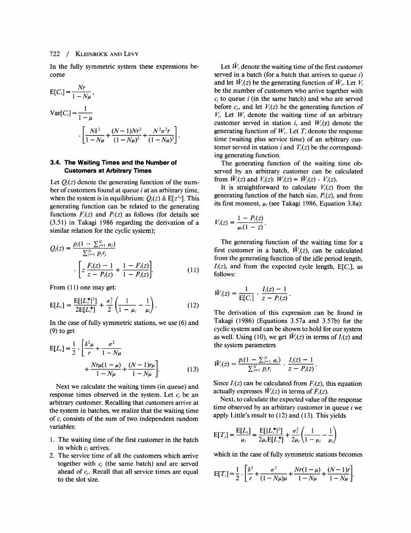
In the fully symmetric system these expressions be- come

E[i] _Nr I- N/'

Var[Ci] =

-N62 (N - l)Nr2 +N 2U2r

+1)2 IN )2].

3.4. The Waiting Times and the Number of Customers at Arbitrary Times

Let Qi(z) denote the generating function of the num- ber of customers found at queue i at an arbitrary time, when the system is in equilibrium: Qi(z) A E[zL]. This generating function can be related to the generating functions F1(z) and Pi(z) as follows (for details see (3.51) in Takagi 1986 regarding the derivation of a similar relation for the cyclic system);

Qi(z) = PiO(1 - X, ,,=)

F Z( (z) 1I+ 1- F_(z)] (11)

From ( 11) one may get:

E[Li]_ EL?1 = -EL). (12)

In the case of fully symmetric stations, we use (6) and (9) to get

1 [62 e' [ r 1 - N1i

Nrpi(1-ut) (N -1)r,i + I N + I - N)r (13)

Next we calculate the waiting times (in queue) and response times observed in the system. Let cj be an arbitrary customer. Recalling that customers arrive at the system in batches, we realize that the waiting time of cj consists of the sum of two independent random variables:

1. The waiting time of the first customer in the batch in which cj arrives.

2. The service time of all the customers which arrive together with cj (the same batch) and are served ahead of cj. Recall that all service times are equal to the slot size.

Let Wi denote the waiting time of the first customer served in a batch (for a batch that arrives to queue i) and let WJ(z) be the generating function of Wi. Let V be the number of customers who arrive together with cj to queue i (in the same batch) and who are served before cj, and let VJ(z) be the generating function of Vi. Let Wi denote the waiting time of an arbitrary customer served in station i, and WJ(z) denote the generating function of Wi. Let Ti denote the response time (waiting plus service time) of an arbitrary cus- tomer served in station i and Tj(z) be the correspond- ing generating function.

The generating function of the waiting time ob- served by an arbitrary customer can be calculated from WJ(z) and VJ(z): WJ(z) = Wi(z) J Vi(z).

It is straightforward to calculate VJ(z) from the generating function of the batch size, Pi(z), and from its first moment, p,i (see Takagi 1986, Equation 3.8a):

1-Pi(z) pHi(l - Z)

The generating function of the waiting time for a first customer in a batch, WJ(z), can be calculated from the generating function of the idle period length, Ii(z), and from the expected cycle length, E[Cj], as follows:

- 1 11(z)-1I -E[Cj] z -P;(z)

The derivation of this expression can be found in Takagi (1986) (Equations 3.57a and 3.57b) for the cyclic system and can be shown to hold for our system as well. Using (10), we get WJ(z) in terms of Ii(z) and the system parameters

J(z) - Pi(l - '= ,) I (z) - 1 E j= I pjrjzPi)

Since Ii(z) can be calculated from Fj(z), this equation actually expresses WJ(z) in terms of F1(z).

Next, to calculate the expected value of the response time observed by an arbitrary customer in queue i we apply Little's result to (12) and (13). This yields

E[Li] E[{L*}2] f ( - -

Ai, 2AiE[Li*] 2Mui -1Ai i

which in the case of fully symmetric stations becomes

1 ^,2 aT2 Nr(-1M) (N-1)r

2 r (i - N,A)t I -N,, I -N,,

The Analysis of Random Polling Systems / 723

3.5. Conditions for Steady State

The scope of this paper is too limited to supply a detailed analysis for the convergence of the system variables to steady state. Nevertheless, since our main results regard the system moments (first and second) at steady state, we now substantiate the conditions under which these results hold. The steady state mo- ments derived in this section are all expressed in terms of f(i) and f(i, j). Therefore, it is sufficient to find conditions under which fi(i) and fi(i, j) are guaran- teed to reach steady state.

The expressions forfm(i) can be obtained by uncon- ditioning (3) and differentiating it with respect to zi. This yields

(i N N'im

fm+'(j) = - * E piri + E

i$j

This relation, which transforms fm(i) to fm+,(i), is shown in Levy (1986) to be a contraction mapping provided that A 1ui < 1. Thus, under these condi- tions, fm(i) is guaranteed to converge independently of the initial values fo(i) and the first moments of the number of customers present in the system at polling instants are guaranteed to reach equilibrium.

The expressions forfm(i, j) are obtained in a similar manner (unconditioning (3) and twice differentiating it). The resulting relation which transforms fm(i, j) to fm+i(i, j) is also a contraction mapping under the condition A 1ui < 1. This condition provides that fm(i, j) will reach steady state. We may therefore conclude that all our results regarding the system moments at steady state hold if E =1I i < 1.

4. Analysis of the Gated Service Policy

As in the exhaustive system, the key to this analysis is the generating function of the number of customers found in the system at the end of a switchover period. This is Fm(Zi, Z2, . . ., ZN), as defined in (1).

For the gated policy, the length of the service period of station i is simply the number of customers found in queue i at the polling instant

ri(m) -Ei(m) = L&Ej(m)).

Thus, the generating function of the number of cus- tomers arriving during this period is given by

E[N ~P(1~r(m-~ EH z)N

fE I {Pj(zj) jTi(rI-,:(rn) = E j) {Pj(z:j).(,n)).

Thus, (3) is replaced by

Fm+i(zi, z2, ..., ZN Ai)

N

*Fm(Zi, z2, * * H i1I PV(Z1), z1+1, * , ZN) 1=1

and (4) is replaced by

F(z, z2, ,ZN)

N

= pi *F(zj, *.. zN X Ai) (14a) i=l1

where

F(zi, . . . ZN IAi)

/N

j=1 ~ j=1

F Fzi, z2,.. *** zi-19 fI Pj(zj), Zi+1,,* * , ZN) (I14b)

Defining the moments of L* (f(i), f(i, j), f(i I k) and f(i, j I k)) as in the exhaustive model and differentiat- ing (1 4b), we get the following set of equations:

f(i I i) = riM + 1ulf(i)

f(i Ii) = ri,ut + 1.tf(i) + f(j) i $ 1.

The solution of these equations (see Levy 1984) is

E[Lj*] = f(i) = i 1r1

When pi = 1/N for every i this is identical to the equivalent expression in the gated system where the polling is done in a cyclic fashion (Rubin and De Moraes). In the case of fully symmetric stations E[L3*] is

E[Lj*] =f(j) = -Nr* (15)

To find the variance of LP we differentiate (14b) twice. This gives the following set of equations:

f(j, k I i)

= /jAk(bi + r?) + riAukf(j) + riujf(k)

+ f (i),jk(2r1 + 1) + f(j, k)

+ Mjf(i, k) + Akf(i, j) + AjAkf(i, i)

i?j,i?k,j?k (16a)

724 / KLEINROCK AND LEVY

f(j, i I i) = Aj(b52 + ri) + ri(?j - Mj) + 2riMjf(j)

? f(i)[Uj2- MUj + Au](ri + 1)]

+f(j,j) + 2,jf(i, j) + Mj2f(i, i) ij $ (16b)

f(i, k Ij)

= IjAUkQ6 + rj2) + rjtjf(k) + f(Ij),jk(2rj + 1)

+ MJf(j, k) + Mj/kf(i,j) jik (16c)

f(i, ilj)

= M](^,5 + rj2) + rj(]j2 _ A

ft(j)[a - Aj + M](2rj + 1)]

+ Aj2f (j j). (I16d)

These equations, together with the relation f(j, k) = E=1 Pi p* f(j, k I i), form a set of N2 linear equations that can be solved by numerical methods (Levy 1986) to yield the solution off(i, i) for i = 1, 2, .. . , N.

In the case of fully symmetric stations this set of equations can be solved analytically (see Levy 1984) to yield

. ._2rN[I - (N- I)Au] (i, i)- (1 + p)(1 -N)2

(62 - r2)N,M2

(1 + M)(1 - NM)

(M + 2r)N2r12 +(1 + ,u)(1 -NM)2

,uNr

(1 + 8)(1 - NM)

M2Nr (1 +,)(1 -NM)2 17)

Now, using (15) and (17) we get

Var_L* _ 62A2N a 2rN[ - (N- I)M] V(1 +M)(1 -N) (1 + /)(1 -N)2

+ (N- I)N,u r (1 + M)(1 -

This is the variance of the number of customers found in queue i at polling instants.

To calculate the cycle time, note that in a gated system the generating function of the cycle length is related to the generating function of the number of customers found in queue i at polling instants as

Fj(z) = C4[Pi(z)]. (18)

From (18) the mean and the variance of the cycle time can be easily calculated:

E[Lf*] I I piri E[C1]= EL E 1

Mi Pi -~M

_ Var[L*] _ E[i]3 Var[C71]-

In the fully symmetric case these become

E[C1 = Nr

1 -NA'

Nv2 + N2of2r

ar[ij] (1 + ,u)(l - NA) (1 + M)(l -NM)2

(N- I)Nr2 (1 + I,)(I - )2

Next the generating function of the number of customers found in queue i at arbitrary moments may be calculated. This is done by using expressions that relate the number of customers found in the system at arbitrary moments to the cycle time and to the number of customers found in the system at polling instants. These expressions have been derived for the cyclic polling system (see, for example, (5.14) and (5.15a) in Takagi 1986) and can be easily shown to hold for our system too. These relations are

Q, (Z) 1 Fi[Pi(z)] - F1(z) (I - z)P,(z) QI(z)=E[Cj] Pi(z)-z 1 -P1(z)

E[L1] - (1 + /i)E[IL*2]

_ ?

iU - 2E[L*] 2Ai.

From these, we can now calculate the expected value of the number of customers found in queue i at arbitrary moments. For a fully symmetric system this value is

2A 2

E[LJ= - + 2r 2(1- N)

+NrM(1 +,t)+ (N- l)rM (19) 2(1-NMu) 2(1-NM) (

To calculate the waiting time in the system, we again recall a relation from the analysis of the cylic polling, gated service system (5.18 in Takagi 1986):

= () z[Ci(z) - F1(z)] E[C.] - (z - P1(z))

The Analysis of Random Polling Systems / 725

which is also valid for our system. From this expres- sion the expected waiting time of a first customer in a batch can be calculated.

Lastly, application of Little's result to (19) yields the expected response time for an arbitrary customer in a symmetric system:

^52 a_2

Nr(1 +,) (N-l)r

_ 2r 2A(l 1-N,u) 2(l1-N,u) 2(l1-N,u)'-

The conditions under which the moments of the system variables reach equilibrium are identical to those of the exhaustive system (namely, ZN= Ai < 1). The arguments supporting this claim are identical to those provided in Section 3.5.

5. Analysis of the Limited Service Policy

5.1. The Expected Response Time in a Symmetric System

As in the previous analysis, the key to this analysis is the generating function of the number of custom- ers found in the system at polling instants. This is Fm(zi, Z2, . . ., ZN), as defined in (1).

To express Fm+i(zi, Z2, ..., ZN) in terms of Fm(Zi, Z2, . .. , ZN), we condition Fm+i(zi, Z2, ..., ZN)

on the station polled during the mth cycle:

Fm+i(Zi, Z2, *.. ZN IAj)

- (J Pi (z)) I (h i PD)

=1 =

* -[Fm(Z I, Z2, * * *, ZN) Zi

-Fm(zi , ... X 0X ... * ZN)]

/N \

+ Ri 1J Pj(zj) ) Fm(Z .(.z . , 0, .. , ZN) (20) \j=l

where Fm(zi,. . . , 0.... ZN) iS Fm(Zi, Z2, . . .,ZN) where the ith element equals zero. The first term of this expression represents the situation where queue i is not empty when polled, so queue j "builds up" during the service slot by a factor of Pj(zj) and one customer is removed from the ith buffer. The second term represents the situation where queue i is empty when polled, so no service period follows this polling instant. In both terms, the factor Ri( jl=1 Pj(zj)) represents the queueing build up during the switchover period prior to the m + 1 st polling instant.

From (20), and under equilibrium conditions, we get the following relation

F(zl,..., ZN)

=Pi R( nl Pj(Zj))

lull Pj(zj) ( Z2 z2, ... , -

+ (1 - H Pj(zj))F(O, Z2, ... ZN)]

+ P2 R2(H Pi(Zi))

f *F(jlz) F(, .,zN)

L HP J ZJ))F(zl * ZN Z2 j=I

+.+ PN .RN( JPj(Zj))

[(J-1 )Z(N9 * X ZN 1

( fI PJ(zj) F(z1, *, ZN-i, ) (21)

ZN j=

In the following, we analyze the fully symmetric system. The analysis approach partially follows the approach used in the analysis of the limited ser- vice cycle system (originally reported in Takagi and Kleinrock 1983); here we extend it to derive the expected response time in the system (this extension was later used by Takagi (1985) to derive the expected response time in the cyclic system). Assuming sym- metry and substituting Z1 = Z2 = ... = ZN = Z in (21) we get

F(z, z, ..,Z)

I-R( jp(z)}N) * P(z) NF(zX, z ... ., Z)

Z ~ + R (p(Z)j N) .I( - jp_Z___

*F(O, z, z,..., z) (22)

where we have used the observation that F(O, Z, Z, ... I z) _ F(z 0,z .,z . (,Z . ,

726 / KLEINROCK AND LEVY

due to symmetry. From (22) we have

F(z, z, . . , z)

R({P(Z)}N1) (Z - P(z)I) 1)-F(O, ,z Z Z Z) z-R({P(z)jN) N pP(Z)IN

Next, we substitute z1 = z and z2 = Z3= .--

ZN = 1 into (21). This yields

F(Z, 1, 1,1...,

[R(P(z)) * P(z) * F(z, 1, 1, ..., 1)- L Z

+ R(P(z)) (I P(Z)) F(O, 1, 1 1)

+ N 1 R(P(z)) * P(z) F(z, 1, 1, ..., 1)

+ R(P(z)) (1- P(z)) * F(z, 0, 1, 1, .. ., 1)] (24)

where we have used the symmetry observations:

F(O, 1, 1, . .. S 1)

=F(1,0, 1,..., 1)

... = F(1, 1, 1,..., 1, ),

F(Z, 0, 1, 1, ..., 1)

=F(z, 1,0, 1,..., 1,1)

= v F(Z, 1, 15..., 1, 1, 0),

PI P2 = PN=

From (24) get

F(z, 1, 1, .., 1)

(N- 1)zR(P(z)) . (1 -P(z)F(z, O, 1,1,... ,1) Nz-R(P(z)) - P(z) . (1 + (N- 1)z)

+R(P(z)) * (z-P(z)) * F(O, 1, 1,..., 1) (25) Nz-R(P(z)) * P(z) (1 +(N-1)z)

The next step is to calculate the probability that an arbitrary queue is empty at polling instants. This probability is given byfo A F(O, 1, 1, .. ., 1). From (23) we may calculate fo (see Appendix C. 1 in Levy 1984):

1 -NA - Nr,i fo

I-NA (26)

Next the expected queue length at polling instants is calculated using two simple relations; the first is

dF(z, z, ..., Z)

az Z=I

=N dF(z 1, 1, .. ., 1) (27) az Z=l

This relation simply states that (at polling instants) the expected number of customers in the whole system is N times the expected number of customers in queue i (i = 1, 2, ..., N). This observation is true due to symmetry. The second relation is

dF(O, z, z, ..., z)

dZ z=1

=(N-1) - F(z,O,1, 1, ... , 1) (28)

which is also true due to symmetry. For convenience let us introduce the additional

notation: f _ dF(z, 0, 1, 1, .. ., 1 )/az I z=l . Differentiating (23) and using (28) we show (see

Appendix C.2 in Levy 1984)

dF(z, z, ..., z)

az Z=I

_(N -I)(I - N)fi 1 - Nu - Nr,u

Nra 2

+ 2(1 - Nu)(l - NA - Nr,u)

+ N2A262 + Nru (29) ~2(1-NA -NrAL) + 2 (29

Differentiating (25) and using (28) we show (see Ap- pendix C.3 in Levy 1984)

N. dF(z, 1, 1, ...,5 1) daz Z=I

-(N- I)N-f,

1 - Ng - Nr,

+ .-( 30 ) 2(1 - N)(l - NA - Nr,)

where v = N * [N2rM3 + N,2(1 -Nuj(52 - r2) -

2NrM2 + (ff2 + M)NrI. Now, using (27) we equate (29) to (30) and solve

(see Appendix CA. of Levy 1984) forf:

(q2 + M)Nr

2(1 -NM) (31)

The Analysis of Random Polling Systems / 727

Substituting (31) back into (30) we finally get an expression for the expected queue length at polling instants

dF(z, 1, 1,..., 1)

(N- 1)(o2 + M)r

2(1 - NM - NrM)

rU2 + 2(1 - Nu)(l - Nu - NrMu)

+ NM262 r1-t

2(1-Nu-NrM) + (32)

Having calculated the expected queue length of queue i at polling instants, we next calculate the expected queue length of queue i right after an arbi- trary customer leaves this queue. Let us denote

Gi _ E[L(t I t is a service completion time at queue i)].

First, since the queue chosen to be polled at a given polling instant is independent of the system status, it is clear that

E[Lj(t I is a service starting time at queue i)]

1 aF(z, 1,1,..., 1) I-fo az Z=

Second, we have

Gi = E[Lj(t I t is a service starting time at queue i)] + M- 1.

Thus, from these two relations and from (26) and (32) we get

(N- 1)(o2 + M)( 1-Nu) 2N,u(l-NMu-NrMu)

ar2 + 2NM(1 - Nu - Nr,u)

NM5262 Ma2

2(1-NMu-NrMu) 2r

+ 2N + 1. (33)

This is the expected queue length at station i right after an arbitrary customer leaves this station.

Next, using Gi, the expected response time (waiting time plus service time) of an arbitrary customer is calculated. To calculate E[Ti] we investigate the num- ber of customers left in queue i behind an arbitrary

tagged customer, say cj. These customers are of two types:

1. Customers who arrive together with cj (in the same batch) but who are queued behind cj.

2. Customers who arrive to queue i during the re- sponse time of cj.

Let Pi be the number of customers arriving to queue i together with cj (the same batch) but queued behind cj; then, the following relation is a direct result of the above observation:

Gi= E[Vr] + . * E[Ti]. (34)

To find E[Vi], we assume that cj arrives at slot t and condition on the number of customers arriving during that slot: E[Vi I Xi(t) = k] = (k - 1)/2. The probability that cj arrives in a batch of size k is given by:

k* Pr[Xi(t) = k]

, l-Pr[Xi(t) =l

Thus, unconditioning E[ V1] yields

00 k- k Pr[Xi(t)= k]

k=V 1 2 k Pr[Xi(t) = l] (2 + M2 2 M

(35) 2,u

Substituting (35) and (33) into (34) we finally get the expected response time of an arbitrary customer in the system

E[T]-_ +2 2

2r 2u(I - Nu - Nr,)

NrU2 + 2,(i - Nu - Nr,u)

(N- l)r N32M

2(1-N,u-Nr,u) 2(1-N,u-Nr,u)

5.2. The Probability of an Empty Buffer

An important measure of a queueing system is the fraction of time that the system is empty. In this subsection we are interested in calculating the proba- bility that a buffer is empty at some specific instants.

The probability that a buffer is empty at polling instants was calculated above as:

Pr[queue i is empty at polling instants]

=F(05 1, 1, ... ., 1) =I- 1NA - Nr

1I N - Nr1i

From this measure it is now easy to calculate the probability that a buffer is empty at switchover times.

728 / KLEINROCK AND LEVY

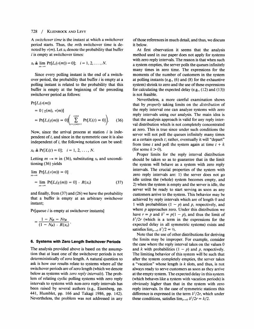
A switchover time is the instant at which a switchover period starts. Thus, the mth switchover time is de- noted by r(m). Let so denote the probability that buffer i is empty at switchover times:

so _ lim Pr[Li(i-(m)) = 0]; i = 1, 2, . . ., N.

Since every polling instant is the end of a switch- over period, the probability that buffer i is empty at a polling instant is related to the probability that this buffer is empty at the beginning of the preceding switchover period as follows:

Pr[L&(r(m))

= 0 l v(m), r(m)] T(m)

= Pr[L&(E(m)) = o] E Pr[X1(t) = O] (36) t =(m)+1

Now, since the arrival process at station i is inde- pendent of t, and since in the symmetric case it is also independent of i, the following notation can be used:

xo A Pr[Xi(t) = 0]; i= 1, 2, ..., N.

Letting m -- oo in (36), substituting so and uncondi- tioning (36) yields

lim Pr[L{r(m)) = 01

-lim Pr[L&(r(m)) =] 0 R(xo) (37)

and finally, from (37) and (26) we have the probability that a buffer is empty at an arbitrary switchover instant;

Pr[queue i is empty at switchover instants]

1 - NA - Nr1 (1 -NA) . R(xo)

6. Systems with Zero Length Switchover Periods

The analysis provided above is based on the assump- tion that at least one of the switchover periods is not deterministically of zero length. A natural question to ask is how our results relate to systems where all the switchover periods are of zero length (which we denote below as systems with zero reply intervals). The prob- lem of relating cyclic polling systems with zero reply intervals to systems with non-zero reply intervals has been raised by several authors (e.g., Eisenberg, pp. 441, Humblet, pp. 166 and Takagi 1986, pp. 142). Nevertheless, the problem was not addressed in any

of those references in much detail, and thus, we discuss it below.

At first observation it seems that the analysis method used in our paper does not apply for systems with zero reply intervals. The reason is that when such a system empties, the server polls the queues infinitely many times in zero time. The expressions for the moments of the number of customers in the system at polling instants (e.g., (6) and (8) for the exhaustive system) shrink to zero and the use of these expressions for calculating the expected delay (e.g., (12) and (13)) is not feasible.

Nevertheless, a more careful examination shows that by properly taking limits on the distribution of the reply interval one can analyze systems with zero reply intervals using our analysis. The main idea is that the analysis approach is valid for any reply inter- val distribution which is not completely concentrated at zero. This is true since under such conditions the server will not poll the queues infinitely many times at a certain epoch t; rather, eventually it will "depart" from time t and poll the system again at time t + k (for some k > 0).

Proper limits for the reply interval distribution should be taken so as to guarantee that in the limit the system will behave as a system with zero reply intervals. The crucial properties of the system with zero reply intervals are: 1) the server does not go idle unless the (whole) system becomes empty, and 2) when the system is empty and the server is idle, the server will be ready to start serving as soon as any customers arrive to the system. This behavior may be achieved by reply intervals which are of length 0 and 1 with probabilities (1 - p) and p, respectively, and where p approaches zero. Under this distribution we have r = p and 62 = p(1 - p), and thus the limit of 32/2r (which is a term in the expressions for the expected delay in all symmetric systems) exists and satisfies limp,o 62/2 = 1/2.

Note that the use of other distributions for deriving the limits may be improper. For example, consider the case where the reply interval takes on the values 0 and k with probabilities (1 - p) and p, respectively. The limiting behavior of this system will be such that after the system completely empties, the server takes a "'vacation" whose length is k slots, and thus, is not always ready to serve customers as soon as they arrive at the empty system. The expected delay in this system (which behaves like a system with vacation periods) is obviously higher than that in the system with zero reply intervals. In the case of symmetric stations this difference is expressed in the term 32/2r, which under these conditions, satisfies limpo0 62/2r = k/2.

The Analysis of Random Polling Systems / 729

The numerical stability of this procedure does not seem to be a problem. This is true although we deal with computing the values of two variables (namely, f(i) and f(i, i) in the exhaustive and gated systems) that vanish to zero. The reason is that in the compu- tation of the expected delay only their ratio appears (see, e.g., (12)), which should not lead to numerical difficulties provided that the relative error in comput- ing each of them is small enough. To examine this issue, we used the proposed procedure (namely, ri = p and V = p(l - p) and letting p approach zero) for several fully symmetric systems and found good agree- ment between the expected delay values computed numerically to the ones derived by taking limits on (13).

It is important to mention that, to the best of our knowledge, cyclic polling systems with zero reply in- tervals have not been analyzed previously under the discrete time model (in contrast, such a treatment was given to the continuous time models, e.g., Cooper and Murray 1969, and Cooper). Thus the method sug- gested here is the only one currently available for analyzing these systems. A more detailed analysis of systems with zero length switchover periods may be found in Levy and Kleinrock (1987).

7. Comparison of the Results and Discussion

In this section, we compare the expected response time in the random polling systems. These results are also compared to the expected response time observed in the corresponding cyclic polling systems.

For the (discrete time) cyclic polling system, we assume the same arrival process as for the random system. The expected response time in the cyclic sys- tem was derived by Konheim and Meister for the exhaustive service policy, by Rubin and De Moraes for the gated service policy and by Takagi (1985) for the limited service policy. (Note that the original expressions derived by Konheim and Meister and extended by Swartz differ from our expressions in two aspects: First, those models assume that arrivals occur at the beginning of a slot while we assume that the arrivals occur at the end of the slot. Second, Konheim and Meister calculate the expected waiting time of the first customer in a batch, while we calculate the ex- pected response time of an arbitrary customer. Note also that the results derived by Takagi (1986) are smaller than ours by one unit because our expressions include the customer service time while his expres- sions do not.) The expressions for the expected response time in the exhaustive, gated and limited service systems can be found in a unified form in Takagi (1986) in Equations 3.61b, 5.21b and 6.64, respectively. These results and the results derived in this paper are summarized in Table I.

Looking at the stability conditions, we see that both the gated and the exhaustive system are stable (under both types of polling methods) as long as NA < 1. On the other hand, the limited service scheme is stable only as long as N,(1 + r) < 1. This result is intuitive since at least one switchover period (whose expected length is r) is associated with every customer served.

Comparison of polling methods shows that for all

Table I Expected Response Time in the Different Systems

Service Polling Method Method Cyclic Random

Exhaustive a 2

2r 2Mu(1-NM) 2r 2M(l - NM)

+ Nr( 1-,) + Nr(l - M) (N- 1)r 2(1-Nii) 2(1-N,u) 2(1-NMN)

Gated 62 2 62 2 _ + , + 2r 2,(2-NMN) 2r 2,u(1--N+)

+ Nr(l + ,) + Nr(1 + ) + (N- 1)r 2(1-NM) 2(1 - NM) 2(1 -Ng)

Limited 62 (1 + Nr)o2 62 (1 + Nr)cT2

2r 2M(N1 - NrM) 2r 2,(1 - N - Nr,u)

+_ NN62M + N62M + (N- l)r +2(1 - N, -Nr,u) +2(1- N,u -Nrii) +2(1 - Ngu-Nr,u)

730 / KLEINROCK AND LEVY

three service policies the expected response time of the random polling scheme is greater than the ex- pected response time of the corresponding cyclic poll- ing scheme. This observation is quite intuitive due to the random behavior of the server in the random polling system. Note also that when the number of stations is N= 1, then the response time in the random system is identical to the response time in the cyclic system.

The difference between the mean response time of the random polling system and that of the correspond- ing cyclic system is (N - 1)r/2(1 - Nq) for the ex- haustive and gated schemes, and (N - 1)r/2(1 - NA - Nr,) for the limited service scheme. In the cases of the exhaustive and the gated systems this difference is exactly the expected length of a period consisting of (N - 1)/2 service periods plus (N - 1)/2 switch- over periods. This difference can be explained as follows. Let to be the time of an arbitrary arrival to queue i. Let t, be the time when the server first starts polling after to. Let t2 be the first time the server polls queue i after to. The period between t1 and t2 consists, on average, of (N - 1)/2 service periods and (N - 1)/2 switchover periods in the cyclic system. On the other hand, this period consists, on average, of N - 1 service periods and N - 1 switchover periods in the random system (this value can be easily calcu- lated by noticing that the number of times the server polls the system unit it hits queue i has a geometrically- shifted distribution with parameter 1/N). Thus, the difference between the expected length of this period in the random system, and the corresponding period in the cyclic system consists of (N - 1)/2 service and switchover periods. Therefore, in the exhaustive and gated schemes the difference in the expected response time between the cyclic and the random systems can be attributed to the period between t, and t2.

Comparing the exhaustive service to the gated service (in both types of polling methods) we see that the expected response time in the gated system is higher. The difference in performance between the exhaustive and the gated schemes is the same for both types of polling methods.

A more difficult task is to compare the limited service to the gated system. In Theorem 1, it is shown that the expected response time observed in the lim- ited service system is greater than or equal to the expected response time in the gated system.

Theorem 1. In the stable random polling system, the expected response time in the limited service scheme is greater than or equal to the expected response time in the gated service scheme.

Proof. Let A be a function representing the difference between the expected response time in the limited service system to the expected response time in the gated system, namely:

A _ TRANDOM; LIMITED- TRANDOM;GATED

(I +Nr)of2 + N__2_ A

2,u(I1-N,u -Nr,u) 2(I1- N,u-Nr,u)

(N-l )r 2(1 -NA2-NrNu)

aCT2 Nr(1 +,u) (N- I)r

L2M(l-NA) 2(1-NA) 2(1 -Nu)_

To prove the theorem, one has to show that A >, 0 for any arbitrary distribution of the switchover period and for any arrival process. By observing that the moments of any discrete nonnegative random variable X (i.e., a variable that takes on the values 0, 1, 2, ...) obey Var(X) > E[X](1 - E[X]) (because E[X2) > E[X]), we have: oU2 > ,(l - A) and 62 - r(I - r). Also, a sufficient condition for stability is easily shown to be Nr,u + N1q < 1. Thus, it is only required to show that A >- 0 for N, r, 62, A and q2 such that: N > 1, Nr1u + NA < 1, a 2 >- (1 - A) and 62 , r(I - r).

First we prove the claim for CT2 = ,(l - ,U) and 62 =

r(1 - r). Rewriting Av we have

(N-2 )r I 2 I -N,u-Nr 1I-Nu-

+- Nr 2

_+ N6

2,u [1-N,u-Nr,u 1-N2

+ Nr2 + ^ 2,(I -NAu-Nru) 2(1 -N,u-Nr,u)

Nr(1+A) (38) 2(I1-N)'(

Using simple inequalities and substituting 2 = ,u(l - ,) and 62 = r(I - r) into (38) we have

>Nr O (-,u),u 2 JI -NA) * (1-N,u-Nr,)

+ 1-Mu + (l-r) I _ +u1 1-N,u-Nr,u 1-N,-Nr, 1-N,J

Nr 1 1-j 2 (1-N,-Nr, 1 -N,u-Nr,u

(I (1r);z _I+

+1-N,u-Nr,u 1-N,u

_Nr (N-1)r1u+2NrAu2 12 O 2 [(I-NA) * (1 -NA-NrA)_

The Analysis of Random Polling Systems / 731

Once the claim A >, 0 is proven for a2 = A(l - A) and 32 = r(l - r), it is now easy to prove it also for 2a , - u) and 62 3 r(l - r). This can be shown by observing that A is monotonically nondecreasing both in U2 and in 62.

Note that the proof of the above result implies an equivalent inequality for the cyclic polling system, namely

TCYCLIC;LIMITED 1TCYCLIC;GATED.

While the expected response time in the cyclic polling systems was derived in Takagi (1985), this inequality for discrete time systems has not been proven previ- ously (note, however, that the inequality was estab- lished for continuous time systems; see for example, Fuhrmann 1985 and Takagi 1985).

We can therefore conclude that for both polling schemes the mean response time increases as we go down the table, i.e.,

TRANDOM;EXHAUSTIVE < TRANDOM;GATED

S TRANDOM;LIMITED

TCYCLIC; EXHAUSTIVE S TCYCLIC;GATED S TCYCLIC; LIMITED

and the mean response time increases as we go across the table, that is,

TCYCLIC;X S TRANDOM;X

where x is any of the service policies.

8. Summary

We have analyzed the performance of random polling systems under three service policies: exhaustive, gated and limited. We derived closed form expressions for the expected response time in all three systems under the assumption of full symmetry. For the nonsym- metric exhaustive and gated systems our analysis yields a set of N2 linear equations the solution of which directly gives the expected response time in the system. Also derived in this paper are expressions for the number of customers in the system, cycle time, intervisit time and buffer utilization.

Appendix: Glossary of Notation

(All time units are measured in slots rather than seconds).

Ai The event that queue i was polled in the previous service period.

c, The ith customer.

Ci, C1(z) The length of a cycle (for a system in equi- librium) and its generating function, respectively.

F(z1, z2, ..., ZN) The generating function of the number of customers found in the system at polling instants.

F1(z) The generating function of the number of cus- tomers found at queue i at polling instants.

Ii, Ii(z) The length of an idle period (in equilibrium) and its generating function, respectively.

L* The number of customers found in queue i at polling instants (system in equilibrium.)

Li(t), Li The number of customers in queue i at time t and in equilibrium, respectively.

pi The probability that station i is polled at a given polling instant.

Pi(z) The generating function of X1(t). Qi(z) The generating function of the number of cus-

tomers found in queue i at arbitrary moments (in equilibrium).

ri The expected length of the switchover period as- sociated with station i.

Ri(z) The generating function of the length of the switchover period associated with station i.

Si, S1(z) The length of a service period (system in equilibrium) and its generating function, respec- tively.

Ti, T1(z) The response time of an arbitrary customer arriving to station i (system in equilibrium) and its generating function, respectively.

VJ The number of customers arriving together (in the same batch) with a tagged customer to queue i and which are served in front of the tagged customer.

VI(z) The generating function of Vi. WV, WJ(z) The waiting time of an arbitrary customer

arriving to station i (in equilibrium) and its gen- erating function, respectively.

xo The probability that no customer arrives at queue i at time t (symmetric system).

Xi(t) The number of arrivals to queue i at time t. 6? The variance of the length of the switchover

period associated with station i.

Ai E[Xi(t)]. a?* Var[Xi(t)].

r(m), r(m), 1(m) The instants at which the mth service period of the system starts, the mth service period of the system terminates, and the mth switchover period of the system terminates, respectively.

ri(m), r-(m), 1i(m) The instants at which the mth service period of queue i starts, the mth service period of queue i terminates, and the

732 / KLEINROCK AND LEVY

mth switchover period of queue i terminates, respectively.

Acknowledgment

This research was supported in part by the Defense Advanced Research Projects Agency of the Depart- ment of Defense under contract MDA 903-82-C-0064. This paper was written while Hanoch Levy was at the University of California, Los Angeles, California. We would like to thank an anonymous referee and the associate editor for making us aware of the issue of polling systems with zero length switchover periods.

References

COOPER, R. B. 1970. Queues Served in Cyclic Order: Waiting Times. Bell Syst. Tech. J. 49, 399-413.

COOPER, R. B., AND G. MURRAY. 1969. Queues Served in Cyclic Order, Bell Syst. Tech. J. 48, 675-689.

DE MORAES, L. F. M. 1981. Message Queueing Delays in Polling Schemes with Applications to Data Com- munications Networks. UCLA-ENG-8106, Depart- ment of System Science, School of Engineering and Applied Science, University of California, Los Angeles, Calif. (May).

EISENBERG, M. 1972. Queues with Periodic Service and Changeover Time. Opns. Res. 20, 440-45 1.

FERGUSON, M. J., AND Y. J. AMINETZAH. 1985. Exact Results for Nonsymmetric Token Ring Systems. IEEE Trans. Commun. COM-33, 223-33 1.

FUHRMANN, S. W. 1985. Symmetric Queues Served in Cyclic Order. Opns. Res. Lett. 4, No. 3, October.

HASHIDA, 0. 1972. Analysis of Multiqueue. Rev. Elect. Commun. Lab. 20, 189-199.

HUMBLET, P. 1978. Source Coding for Communication Concentrators. Electronic Systems Laboratories, Massachusetts Institute of Technology, Cambridge, ESL-R-798 (January).

KONHEIM, A. G. 1980. Mathematical Models for Com- puter Data Communication. In Case Studies in Mathematical Modeling, pp. 256-334, W. E. Boyce (ed.). Pitman Advanced Publishing Program, Boston, Mass.

KONHEIM, A. G., AND B. MEISTER. 1974. Waiting Lines and Times in a System with Polling. J. Assoc. Comput. Mach. 21, 470-490.

LEVY, H. 1984. Non-Uniform Structures and Synchro- nization Patterns in Shared-Channel Communica- tion Networks. CSD-840049, Computer Science De- partment, University of California, Los Angeles, Ph.D. dissertation (August).

LEVY, H. 1986. Delay Computation and Dynamic Be- havior of Non-Symmetric Polling Systems. AT&T Bell Laboratories, Holmdel, N.J., February 1986. Submitted for publication.

LEVY, H., AND L. KLEINROCK. 1987. Polling Systems with Zero Switch-Over Periods: A General Method for Analyzing the Expected Delay. AT&T Bell Lab- oratories, Holmdel, N.J. (June).

NOMURA, M., AND K. TSUKAMOTO. 1978. Traffic Analy- sis of Polling Systems (in Japanese). Trans. Inst. Electron. Commun. Eng. Jap. J61-B(7), 600-607.

RUBIN, I., AND L. F. M. DE MORAES. 1983. Message Delay Analysis for Polling and Token Multiple- Access Schemes for Local Communication Net- works. IEEE. J. Select. Areas Commun. SAC-1, 935-947.

SWARTZ, G. B. 1980. Polling in a Loop System. J. Assoc. Comput. Mach. 27, 42-59.

TAKAGI, H. 1985. Mean Message Waiting Times in Sym- metric Multi-Queue Systems with Cyclic Service. Perform. Eval. 5, 271-277.

TAKAGI, H. 1986. Analysis of Polling Systems, MIT Press, Cambridge, Mass.

TAKAGI, H. 1987. A Survey of Queueing Analysis of Polling Systems. In Proceedings of Third Interna- tional Conference on Data Communication Systems and Their Performance, Rio De Janeiro (June).

TAKAGI, H., AND L. KLEINROCK. 1983. A Tutorial on the Analysis of Polling Systems, University of Cali- fornia at Los Angeles (December). (A preliminary draft of Takagi and Kleinrock 1985a, b, and Takagi 1986).

TAKAGI, H., AND L. KLEINROCK. 1985a. Analysis of Polling Systems. IBM Japan Science Institute, TR87-0002 (January).

TAKAGI, H., AND L. KLEINROCK. 1985b. Analysis of Polling Systems. University of California at Los Angeles, CSD-850005 (February).