Author(s) Davis, Michael Chase Title Massachusetts Institute

Calhoun: The NPS Institutional ArchiveDSpace Repository

Theses and Dissertations 1. Thesis and Dissertation Collection, all items

1961-06-01

Optimum systems in multi-dimensionalrandom processes.

Davis, Michael ChaseMassachusetts Institute of Technology

http://hdl.handle.net/10945/12782

Downloaded from NPS Archive: Calhoun

LIBRARY

US NAVAL POSTGRADUATE SCHOOL

MONTEREY CALIFORNIA

OPTIMUM SYSTEMS

IN

MULTIDIMENSIONAL RANDOM PROCESSES

by

MICHAEL CHASE DAVIS

Lieutenant, U.S. Navy

B.S., U.S. Naval Academy

(1953)

SUBMITTED IN PARTIAL FULFILLMENT

OF THE

REQUIREMENTS FOR THE DEGREE OF

DOCTOR OF SCIENCE

at the

MASSACHUSETTS INSTITUTE OF TECHNOLOGY

June, 1961

Signature of Author ---._ = -_-~.-'_~-~~---~--_--., _ = _

Department of Electrical Engineering, May 13, 1961

Certified by ------ - - ____-__-_---_-_-___-_-_--_Thesis Supervisor

Accepted by - -_= ------------------------------- -Chairman, Departmental Committee on Graduate Students

\°i<o\,0<o

PAv/xs^M-

Library

U. S. Naval Postgraduate School

Monterey, California

OPTIMUM SYSTEMS IN

MULTI-DIMENSIONAL RANDOM PROCESSES

by

MICHAEL CHASE DAVIS

Lieutenant, U. S. Navy

Submitted to the Department of Electrical Engineering on May 13, 1961,

in partial fulfillment of the requirements for the degree of Doctor of Science.

ABSTRACT

This thesis deals with random processes which are stationary,

ergodic, and described by correlation functions or power density spectra.

An attempt has been made to develop a new approach to the study and control

of random processes which is simple, stresses physical rather than mathe-matical interpretation, and is valid when a number of statistically related

processes are to be processed simultaneously. Among the origianl and fun-

damental results of this investigation are:

(1) A closed-form solution is presented for the optimum multi-di-

mensional system in the Wiener sense. This system operates on n correlated

random input signals and produces m desired outputs, each of which hasminimum mean-square error. The solution is dependent upon the factoriza-

tion of a matrix (f)(s) of the cross -power density spectra of the input signals

into two matrices, such that <J)(s) = G(-s) . GT(s). The nxn physical systemG(s) determined from this procedure must be realizable and inverse realizable,

and is the system which would reproduce the measured statistics when excited

by n uncorrelated white noise sources.

(2) A general solution is derived for the above matrix factorization

problem, valid without regard to order, providing the spectra satisfy a

realizability requirement. The method employs a series of simple matrixtransformations which manipulate the original matrix into desired forms.The key to this solution is a general procedure for reducing a matrix with

polynomial elements to impotent form, having a constant determinant. Thislatter step is also an original contribution to the theory of matrices with

algebraic elements. With this solution to the matrix factorization problem,essentially no conceptual difference remains between single and multi -di-

mensional random processes.

(3) The optimum single or multi -dimensional prediction operation is

-li-

shown to result from a continuous measurement of the current state

variables of the hypothetical model G(s) which can create the random pro-

cess from white noise excitation. These state variables are then weighted

according to their decay as initial conditions in the desired prediction timeand the"decayed "output or outputs are the desired prediction. Thus, ex-

pected behavior of the random process over all future time is compactlysummarized in the current values of these state variables.

(4) It is proved that correlation functions measured between twovariables in a linear system can be viewed as an initial condition responseof this system. Also, the well-known Wiener-Hopf equation is shown merelyto require that every error be uncorrelated with past values of every input

signal.

(5) If one or more noisy signals have a power density spectra matrix(y (s), which can be factored into G(-s) GT (s), and if G(s) is separatedsuch that G(s) = S(s) + N(s), where S(s) and N(s) have signal and noise poles,

respectively, then it is shown that the optimum filter is a unity feedbacksystem with forward transference S(s) N~ (s). This very general result is

valid for single or multi -dimensional optimum filtering problems.

(6) A quantitative substitute for the Nyquist sampling theorem is

presented which is concerned with a measure of the irrecoverable error in-

herent in representing a continuous random process by its samples. Also,

the new results in continuous random process theory derived herein are ex-tended to the discrete case.

(7) The concept of "state" of a random process is advanced as

fundamental information for control use. Two new design principles arediscussed for the bang-bang control of a linear system subject to a randominput. In one, suitable for multi -dimensional full throw control, the deter-minate Second Method of Lyapunov is extended to include random processes.

The basic contributions of this thesis are (1) a complete theory of

multi -dimensional random processes, (2) a simple physical explanation for

the optimum linear filter and predictor using white-noise generating models,and (3) a new approach to stochastic control problems, especially thoseinvolving saturation, using the concept of the "state" of a random process.

Thesis Supervisor: Ronald A. Howard

Title: Assistant Professor of Electrical Engineering

-in-

ACKNOWLEDGMENT

The author is very grateful to Professor Ronald A. Howard for

his support and encouragement throughout this research, and to LCDR

John R. Baylis, USN and Professor Amar G. Bose for their valuable

assistance.

To Captain Edward S. Arentzen USN and Professor Murray F.

Gardner, thanks are due for their active encouragement during the entire

doctoral program. The author is indebted to the Bureau of Ships, U. S.

Navy, for providing the financial support which made this investigation

possible.

The author is appreciative of the competency of Mrs. Jutta Budek,

who performed the final typing of this manuscript.

Finally, the author wishes to thank the "unsung heroine", his wife

Beverly, for her gracious acceptance of the trying demands of the thesis

research and presentation.

-IV-

TABLE OF CONTENTS

CHAPTER I.

CHAPTER H.

CHAPTER HI.

Page

INTRODUCTION 1

DERIVATION OF OPTIMUM SINGLE ANDMULTI-DIMENSIONAL SYSTEMS2. 1 Introduction 4

2. 2 Historical perspective 4

2. 3 Summary of linear statistical theory 5

2. 4 A general formula for power density

spectra transformations 10

2.5 Single-dimensional optimum systems 13

2. 6 Multi-dimensional optimum systems 20

2. 7 Past attempts to determine optimummulti -dimensional system 23

2.8 A new closed-form solution for anoptimum multi -dimensional system 28

2. 9 Statistical transformations on randomvectors 31

MATRIX FACTORIZATION3. 1 Statement of the problem 35

3. 2 Realizability considerations 36

3.3 Two special cases 39

3. 4 Properties of matrix transformations 42

3.5 Matrix factorization: A general solu-

tion 44

3. 6 Matrix factorization: An iterative

solution 55

3. 7 Matrix factorization: A lightning

solution 60

3. 8 Statistical degrees of freedom of amulti -dimensional random process 63

CHAPTER IV. NEW RESULTS IN OPTIMUM SYSTEM THEORY4. 1 Introduction 68

4. 2 Matrix differential equations andsystem state 69

4. 3 Interpretation of the optimum linear

predictor 72

4. 4 A quantitative measure of samplingerror for non-bandwidth limited signals 80

4. 5 New results and interpretations for the

optimum filtering problems 84

TABLE OF CONTENTS (CONT.

)

4. 6 Correlation functions and initial

condition responses4. 7 Advantages of the state and model

appraoch to random processes

Page

92

95

CHAPTER V. RANDOM PROCESSES AND AUTOMATICCONTROL5. 1 Introduction 98

5. 2 Saturation and control in a stochastic

environment 99

5.3 Optimum feedback configurations with

load disturbance 108

5.4 Contemporary designs for full throwcontrol of a system subject to a randomprocess 110

5. 5 Multi -dimensional bang-bang control of

systems subject to random processinputs 112

CHAPTER VI. SUMMARY AND CONCLUSIONS6. 1 Outline and summary6. 2 Paths for future research

120

123

APPENDIX I. OPTIMALITY IN DISCRETE LINEARSYSTEMS1. Introduction 127

2. Fundamental properties of discrete

signals and systems 127

3. Statistical relationships 128

4. Optimum configurations 129

5. Special interpretation of optimum systems

6. Considerations for optimum linear

sampled-data control systems7. Conclusions

130

132

134

APPENDIX II. A 3x3 EXAMPLE OF MATRDC FACTORIZATION1 jo

BIBLIOGRAPHY

BIOGRAPHICAL NOTE

141

144

-VI'

CHAPTER I.

INTRODUCTION

The word "random" is an adjective which mankind has come to

use in apology for unwillingness or inability to measure fundamental

causes for events observed in Nature. Of these events, the random

process which goes on continuously and indefinitely has captured the

interest of mathematicians and engineers. There is something com-

pelling about attempting to describe that which is ever changing, and

thus undescribable.

This thesis is concerned with random processes in their sim-

plest form -- with statistics that do not change with time, and whose

properties are adequately described by the well-known correlation

functions. Many able researchers have cleared this path and it could

well be asked, like an echo from the Second World War, "Is this trip

necessary?"

To begin with, a research investigation is generally based on

aggravation, either with what is not known or with what is known. In

this work, the latter case is true. It is the opinion of the author that

the classic and beautiful core theory of Wiener in this area, by its

very mathematical eloquence, has tended to suppress a more funda-

mental understanding of what can be known in a random process and

what cannot.

In essence, the original work of this thesis starts with the

well-known fact that the random processes considered here act as if

they came from a linear system which is excited by the most random

of signals, "white" noise. This linear system specifies the particular

random process, and focussing attention on its determinate structure

is a more satisfying approach, at least to the engineer, than is ac-

cepting the manipulation of statistical properties of the ever-changing

output of this system.

Some of the unsolved problems and prominent possibilities in

-1-

random process theory which come to mind for possible attack are:

(1) Conventionally, derivations in the Wiener theory are made

for optimum systems in the time domain. A pure transform approach

appears much more desirable.

(2) A general closed-form solution for the optimum multi~di-

mensional system has not yet been given in the literature.

(3) A means has not yet been found for determining a physical

system capable of reproducing signals with the given statistics of mul-

ti-dimensional random processes.

(4) The fundamental results of Wiener theory are the optimum

predictor and filter. It may be possible that these have a very simple

interpretation in terms of the equivalent white -noise driven system.

(5) The correlation functions of many observed random pro-

cesses have the appearance of an initial condition response of a linear

system. If this is true, what linear system and what initial conditions?

(6) What effect would white ntiise have if suddenly applied to an

otherwise quiescent linear system?

(7) There is no valid measure of the inherent error due to sam-

pling of a random process to replace the "Go-No Go" nature of the

Nyquist Sampling Theorem.

(8) If a linear theory produces all the knowable information

about an input random process, is there some way of intelligently

using this to control a physical system which has limitations such as

saturation? No suitable approach to the on-off or bang-bang control

problem with random excitation has been made which makes complete

use of this information.

(9) If a random process is to be examined by means of inves-

tigation of an effective physical system, can some determinate ap-

proaches to systems analysis such as the "Second Method of Lyapunov"

be extended to include random processes ?

This thesis provides a quantitative answer to each of these ques-

tions or possibilities. The author believes that the results found in this

-2-

thesis investigation, because of their simplicity and generality, provide

the most effective means for understanding the nature of stationary ran-

dom processes.

-3-

CHAPTER II.

DERIVATION OF OPTIMUM

SINGLE AND MULTIDIMENSIONAL SYSTEMS

2. 1 Introduction

This chapter is concerned with linear systems which operate on

stationary random processes so as to minimize a quadratic measure of

error between the desired and actual outputs. In the case of a single ran-

dom signal, perhaps corrupted by noise, the results of this theory have

been known for over a decade. Why, then, is it necessary to retrace

such well-worn steps?

There are two reasons for this apparent duplication. First of

all, the author feels that the time -domain derivations found in many

standard texts of the optimum Wiener filter are unnecessarily compli-

cated and tend to obscure the basic simplicity of the ideas expressed.

Secondly and more important, when the optimum system to process two

or more signals simultaneously is derived, the conventional methods

rapidly become enmeshed in their own symbology, whereas the steps of

the single -signal frequency domain approach to be described in this

chapter allow direct extension to the multi-dimensional case.

2. 2 Historical perspective

In this country, the origin of the statistical theory of optimum

linear systems was the wartime work of Wiener . A parallel develop-

ment in Russia at approximately the same time was made by Kolmogorov

The structure of the basic theory was thus well-formed by 1950 for prob-

lems involving prediction and filtering of a single stationary random pro-

cess in the presence of additive noise. Significant extensions and clari-

3fication of Wiener's work were made by Zadeh and Ragazzini , Bode

4 5 6 7 8and Shannon , Blum , Lee , Pike , and Newton . The latter' s work

was of particular significance, since it introduced the concept of optimi-

zation with constraints in order to satisfy certain practical engineering

-4-

2

requirements of a system which the basic theory neglected. In the last

decade, graduate -level control systems engineering texts have gener-9

ally emphasized the statistical approach. These include books by Truxal,

Newton , Smith , Seifert and Steeg , and Lanning and Battin .

In the multi- dimensional case, the theory is not as well-developed.

14Westcott derived an optimum configuration for the two-dimensional

15case. Amara ' used a partial matrix approach and successfully derived

the optimum unrealizable configuration, but his realizable solution was16

only applicable upon very restricted signal conditions. Hsieh and Leondes

presented a method for solving for the optimum system involving unde-

termined coefficients, but the meaning of their solution was obscured

by the formidable notation employed and no proof of the adequacy of

their method was offered.

2. 3 Summary of linear statistical theory

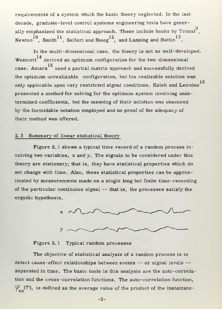
Figure 2. 1 shows a typical time record of a random process in-

volving two variables, x and y. The signals to be considered under this

theory are stationary; that is, they have statistical properties which do

not change with time. Also, these statistical properties can be approx-

imated by measurements made on a single long but finite time-recording

of the particular continuous signal -- that is, the processes satisfy the

ergodie hypothesis.

Figure 2. 1 Typical random processes

The objective of statistical analysis of a random process is to

detect cause -effect relationships between events --or signal levels --

separated in time. The basic tools in this analysis are the auto -correla-

tion and the cross -correlation functions. The auto -correlation function,

Y (T), is defined as the average value of the product of the instantane-

-5-

ous signal and the signal level \ seconds later.

^ xx(T) i E |x(t) * x(t+r)| (2.1)

where the symbol — is a defining equality and the operator E^» } means

"the expected value of". Expressed in integral form for the class of

signals considered,

^xx(r)=T^>2T f* *>'.«t+T> (2.2)

Figure 2. 2 shows a typical auto -correlation function. Note that

it is even about the'T^= axis, ^f(f) =^f

(-T"'), since replacing t by

t -T in Equation 2. 2 does not affect its value. The maximum value of

y (T) is at T= for any stationary signal observed in the real worldxx

9(a proof is given by Truxal .

)

The cross -correlation function, iP (T), is defined as the average

value of the product of the instantaneous signal level of one variable, x,

and that of another signal, y,T' seconds later.

^ xy<r) i E Lit)' y<t+r>j

I xvxylim J^T-»°£> 2T

dt X(t) • y(t +r>

(2.3)

(2.4)

ft. (r )

Figure 2. 2 A typical auto -correlation function

In this case, replacing t by t -fin the integral form yields the

definition of LD (=T ), and the peak value of IP ( T' ) does not necessar-

ily occur at the origin. Summarizing,

-6-

y <-r> = V m (2.5)' XX 'XX

if (-T) = if (T) (2.6)T Xy / yx

The auto -correlation functions and all possible cross -correla-

tion functions among members of a set of random signals completely

describe the particular process for the purposes of a linear theory.

One significant use of the auto -correlation function is that Y (0)

is, by definition, the mean square value of x. For example, this makes

it a useful measure of the accuracy of a system when the signal concerned

is the error.

Since the correlation functions (for'T~/>0) have the same appear-

ance as transient signals observed in linear systems it is logical to de-

fine the Laplace transforms of these functions and inquire as to their

potential use. As the functions are defined for both positive and nega-

tive T* , the bilateral or "two-sided" Laplace transform is selected for

use. The bilateral Laplace transform evaluates the positive -time part

of a signal just as the one-sided Laplace transform does, but the nega-

tive-time portion has the sign of t changed (i e: "flipped over" the t =

axis), evaluated as a positive -time signal, and the sign of s, the trans-

form variable, is changed to -s.

In order to ensure a one-to-one correspondence between the trans-

form and the time -domain expression, it is necessary to specify that all

poles in the right half plane (or "negative" poles) correspond to functions

in negative time and not unstable functions in positive time.

In this work, the bilateral Laplace transform of the auto and

cross -correlation function is defined as the auto or cross power density

spectrum, Q) (s) or (£ (s), respectively. The notion of power density

arises in the following fashion:

The mean square value of a random signal x is envisioned as a

generalized form of average energy because of its quadratic nature, and

is equal by definition to if (0) . If If (0) is finite, it is equal to the

-7-

sum of the residues of either the left- half or right -half plane poles of

the transform (s), as seen directly from a partial fraction expan-

sion of (s) and term -by-term inversion. But by the residue theorem

of complex variable theory, the evaluation of a closed contour up the

imaginary axis of the s -plane and enclosing the left -half-plane at infin-

ity will yield 2irj x summation of residues, providing the contour is of

the order of no less than -5- as s —*©o. That is, vj) (s) must contain

s

at least two more poles than zeros for a finite mean square value,*f

(0),

to exist.

Thus,

P=<°> 5j f*

©0

is <5xx

(s) (2.7)

-ioO

Let s = jw

xx 2n xx

The mean square value (or power) of a signal is thus seen to be

proportional to the integral of , and W (w) quite natu-Xa X..X.

rally is visualized as a power density per unit u, Most authors have in-

cluded the — in the definition of the power density spectrum so that

the integral over all w yields the total average power, but this appears

to be less natural than retaining the pure transform relationship, espe-

cially since the name "power" is a misnomer in itself. The u notation

is the most common encountered in past literature on random processes,

and brings to mind a weighting of harmonic content, considering the ran-

dom process to be a superposition of an infinite number of infinitely small

simusoidal waves.

It might be argued that the choice of nomenclature is a trivial

matter, but in as much as it influences basic conceptualization of a ran-

dom process, it is very important and deserves elaboration.

Ten years ago in automatic control literature, the transfer function

-8-

of a linear system was invariably written as G(jto), and much was made

of plots of frequency response on polar or logarithmic coordinates. Fre-

quency response was almost regarded as an end in itself, and design

specification in terms of these characteristics helped propagate this

17belief. However, the acceptance of Evan's root-locus method and the

gstrong emphasis by Truxal and others towards use of the Laplace

transform helped unify the differential equation, frequency response,

and transient response approaches to dynamic behavior of linear systems.

In proper perspective, frequency response is an often desirable experi-

mental description of a system and provides, on logarithmic coordinates,

a rapid means for design of simple control systems when specifications

on transient behavior are loose. Frequency response is perhaps best

visualized as an imaginary axis scan on the complex plane, as shown in

Figure 2. 3, where the function is evaluated by the complex product of

vectors from all system zeroes divided by vectors from all system poles

to the particular s = jco point under consideration.

s - PLANE

Figure 2. 3 Frequency response viewed as imaginary axis scan

Since linear systems were previously regarded in terms of how

they altered the magnitude and phase of an input sinusoidal signal, essen-

tially a communications engineering viewpoint, it is natural that random

processes should have been described in terms of relative frequency

content. But now that the Laplace transform -- high-lighting the system

poles and zeroes -- has emerged as perhaps the best index to the prop-

erties of a linear system, it is necessary to take the viewpoint in a ran-

dom process that the characteristics of interest are the poles and zeroes

of the power density spectrum §) (s), and not necessarily the spectrum

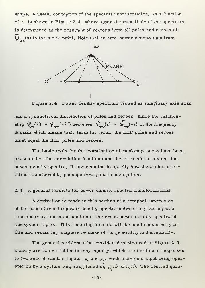
shape. A useful conception of the spectral representation, as a function

of w, is shown in Figure 2.4, where again the magnitude of the spectrum

is determined as the resultant of vectors from all poles and zeroes of

(I) (s) to the s = jw point. Note that an auto power density spectrum

JOJ

Figure 2. 4 Power density spectrum viewed as imaginary axis scan

has a symmetrical distribution of poles and zeroes, since the relation-

ship & CO = W (-7s") becomes <P (s) = <P (-s) in the frequency

XX 'XX xx xxdomain which means that, term for term, the LHP poles and zeroes

must equal the RHP poles and zeroes.

The basic tools for the examination of random process have been

presented ~ the correlation functions and their transform mates, the

power density spectra. It now remains to specify how these character-

istics are altered by passage through a linear system.

2.4 A general formula for power density spectra transformations

A derivation is made in this section of a compact expression

of the cross (or auto) power density spectra between any two signals

in a linear system as a function of the cross power density spectra of

the system inputs. This resulting formula will be used consistently in

this and remaining chapters because of its generality and simplicity.

The general problem to be considered is pictured in Figure 2.5.

x and y are two variables (x may equal y) which are the linear responses

to two sets of random inputs, x. and y., each individual input being oper-

ated on by a system weighting function, g.(t) or h.(t). The desired quan-

-10-

X,

x^

>-

y-1

•

•—-—> > iw .

» "IS^

^—-»-1

X

y*-

*

'/m.-*-

> Kj(±) ^y

Figure 2. 5 General model for linear system

tity is (y (s); the known quantities are the cross -power density spectra

between any two of the inputs x. and y..

x(t) = Z. g.(t)*x.<t) ; y(t) » 5.-L=/

X XJ-/

where "-# " is a symbolic operator expressing convolution. Transform-

h.(t)* yjJ J

mg,

Xls] = > G.(s) X.(s)i i

/WV»

Y(s) = ^> H.(s) * Y.(s)

*•=/ J= i

+r>

= Et 1

x( dC £y(t+r)]

assuming that the integration involved with averaging in time can

commute with the integration of the Laplace transform. The subscripts

on the operator indicate the time variable which is used in the opera-

tion.

-11-

Consider a length of signal which exists for duration 2T, where

T is arbitrarily large but finite,, and which is zero elsewhere.

T T

xy(s) =

T^°-k Jdtx(t)/y(t+r)e"-sT

'dr

-T

T->«o 2T J dt x(t) eSt

y(s)

-T

lim 1

X-x=o 2TX(~s) * Y(s)

34which is a standard result found, for example, in Rice and Solodov-

1135

nikov

But, substituting the values of X(-s) and Y(s),

xy< S

> T^> Tt| IGi<-

S > H/

S> V S)

lim X.(-s) Y.(s)-I I G.(-s) H.(s)

"*-! J-l

G.(-s) H.(s)i J

T->«o — J

2 T

. .(s) (2.9)xi yj

which is the desired result. Several examples will illustrate the con-

venience of this formula.

Consider first the system of Figure 2. 6.

Xcs)—^ Wis) —y yes)

Figure 2.6 A simple linear system

X(s) = X(s) ; Y(s) = X(s) ' W(s)

<D (s) = W(s) 5? (s) (2.10)xy xx

-12-

a basic result which has immediate practical consequences. If x and y

are the available input and output signals of an otherwise inaccessible

system, the system transfer function can be determined without intro-

ducing test disturbances by analyzing the cross -correlation between

x and y.

Also,

2 (s) = $ (s)w(s) ^~s)yy xx

Next, Figure 2. 7 shows a typical summing operation.

X(3)

(2.11)

ZCs)

Figure 2.7 A typical summing operation

Z(s) = X(s) * G(s) + Y(s) H(s)

$ (s) = $ (s)G(~s)G(s) + $ (s)G(=s)H(s) +xy

$ (s)H(-s)G(s) + (E> (s)H(=s)H(s)yx J yy

(2.12)

which is obtained by inspection by performing the necessary cross

-

multiplication and observing the proper sign of s.

2. 5 Single-dimensional optimum systems

The classical Wiener theory of an optimum linear system to

operate on a random process will now be derived using transform ex-

pressions wherever possible. This clear and direct approach is useful

in its own right but is basically intended to provide an introduction to

a similar development for multi -dimensional systems to follow.

Figure 2. 8 shows the basic configuration to be studied. The

stationary input random signal v in general will contain a signal to be

operated on and an extraneous noise component. The ideal signal i is

13-

IDEAL

INPUTW(s) *& —

>

E£ROR

Figure 2. 8 Configuration of an optimum system

the mathematical result of some desired operation on the signal compo-

nent of the input, such as filtering, prediction, or some linear function

of the signal. Figure 2.9 shows an elaboration of this structure, where

. =*- Gr.CS)^r^Vi

5 + /o V. W(s)

ew ~" Mo' V-

/n.

Figure 2. 9 Formation of the ideal signal

the signal component s is operated on by some not-necessarily physi-

cally realizable transfer function, G ,(s), such as 1, e , or s. If $Q SS

and <£^ are known, and since

is) = <£ G,(s) + ~§ G,(s) (2.13)ri ^ss d ns d

Q ,(s) is as equally valid a statistical description of the desired opera-

*.

tion as is specification of G ,(s).

The error signal, e, is the difference between the actual response

of the system to be determined, W(s), and the ideal signal. The optimum—2~

system will minimize the mean value of error squared, e ~ j (0),

which is a satisfactory error criteria for many purposes. The use of

the variance of the first probability distribution of error is a natural

choice when longtime properties of signals are being examined, as a

more complex error criterion besides being mathematically intractable

13would require more statistical knowledge of the processes involved.

-14-

7' ^ee<0) -h j ds $

oO

it] J -1- ee

-j-o

E(s) = I(s) - V(s) W(s)

$ ee(s) = <£..(s) - ^ iv

(s) W(s) - 3>vi

(s) W(-s) +

$vv(s) W(s) W(»s)

The determination of the optimum W(s) in order to minimize the

integral expression is the standard problem of the calculus of variations.

If a perturbation in W(s) is made, called a variation, a resulting pertur-—

jo-

bation or variation in e results.. More formally, W(s) is replaced by

W(s) + 6 ^W(s), where € is a "small" constant and the variation ^W(s)

is any allowable change in W(s), or alternately any system which could

be paralleled with W(s). This restricts cfW(s) to have the properties of

physically-realizable and stable systems, that is, with no poles in the—ir

right-half plane. Also, for a finite e , cfw(s) must not be of such order

as to provide a component of white noise at e when excited by v. e is

then expanded as a power series in 6 around 6 = 0. The optimum system

will have been found when the coefficient of the first power of 6 is zero

regardless of the form of <jW( s ) "-in other words, no small allowable

change in W(s) tends to decrease the value of the integral.

<F7 -1-27TJ

assuming that differentiation may be performed under the integral sign.

The variational notation will now be shown to follow the usual

rules for differentiation, considering the individual terms of Q (s)

consecutively.

/ P>>]

-15-

€=

S pj5. (s)W(s)l = <£ (s) 3^- fw(s) + 6 ifw(sL n= 3>

4(s) cfw(s)Liv J lvd^L Jr=0 iv

cT f^ .(s) W( s)l = $ .(s) -A- fw(-s)+€</w(-s2l = £ .<s) cfw(-s)•- vi -• vi 06 L -i vi

<r[$^s)w(s) W(-s)] = $^) -J—<[w(s)+^W(sjj[W(-s)+€/w(-s|r

= $£) [/w(s)W(-s) + W(s)cTw(-s)]

The only restriction on this analogy with differentiation is that the

variation of W(s) or W( s) must carry the proper sign of s.

JOO

S e2 =0=-V| dsVl. (s)/w(s) - $ .<s)«fw(-s)

27T] I \_IV "''VI

+ !§£) [w(-s) <fw(s) + W(s)<fw(-s) y

To simplify this expression, several auxiliary results are needed.

(1) <5. (-s) =$ .(s), from the fact that (?. (^T) = 9 .01, Equation 2. 6.^ iv -^ vi iv vi

(2) The sign of s may be changed in any single term of the above integral,

without affecting its value, since the limit exchange and the sign change

of the differential ds have cancelling effects.

Changing the sign of terms as necessary to be able to factor dW(-s)

and identifying 35, (-s) as Q> .(s) and JT (s) as $ (-s) .^ IV VI w vv

-)•«

X~"2 1c e ds : r-W(-s) I - <£> .(s) + ($)($) W(s)|

L vi J w J27TJ J

If the integral exists and the contour is selected so as to enclose

the left -half plane, the LHP residues must sum to zero for arbitrary

o W(-s), which has all its poles in the right =half plane. Obviously, the

function I $ (?) W(s) - $ .(s)J must have no simple poles in the LHP,

say at s = - a., for the sum of residues is £ oW(a„) , an arbitrary

number for arbitrary <Jw(-s). If this function has a multiple pole, say

/—I

—

V&:— > then <JW(~s) could be selected so as to include a m-1

order zero at s = - a (only poles must be in the RHP), leaving the first

-16-

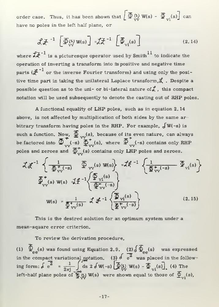
order case. Thus, it has been shown that / W &) W(s) - Q .(s)J canL vv vi J

have no poles in the left half plane, or

J*' 1

[jtJ|W«l] vf*"1

(Xi(B>3 (2.14)

-f?2."l 11where #\oT is a picturesque operator used by Smith to indicate the

operation of inverting a transform into its positive and negative time

parts (^ or the inverse Fourier transform) and using only the posi-

tive time part in taking the unilateral Laplace transform, 5C . Despite a

possible question as to the uni- or bi-lateral nature of^ , this compact

notation will be used subsequently to denote the casting out of RHP poles.

A functional equality of LHP poles, such as in equation 2. 14

above, is not affected by multiplication of both sides by the same ar-

bitrary transform having poles in the RHP. For example, J~W(-s) is

such a function. Now, 

5vi<

S >

}

W(s)1 ££~ l / ^vi

<S)\ (2.15)

$ + (s) ~ * flf (-S)-r vv I x. w

This is the desired solution for an optimum system under a

mean-square error criterion.

To review the derivation procedure,

(1) & (s) was found using Equation 2.9. (2)<4 O (s) was expressedee ___. ee

in the compact variational notation. (3) o e was placed in the follow-

ing form: £ e2

= -^K~ J ds 2 J"w(-s) [_J^ W(s) - $ .(s)]#

(4) The

left -half plane poles of "^ (S) W(s) were shown equal to those of Q .(s),

17-

and both sides of this equality were multiplied by the inverse factor of

3>*"

(-s).wAn example of this procedure is given next to illustrate the ease

in derivation of extensions to the basic theory. This modification is dueO

-J f\

to Newton ' and is an attempt to control saturation in a given power

transducer. Figure 2. 10 shows that a signal driving a fixed element

G (s) isP

e-V-

6,C«)c

>• ^

V W(s) GfW W>H 9* ~v

FIXEDELEMENTS

Figure 2. 10 Control of saturation in fixed elements

to have some linear function (G (s) usually equals 1, s, or s ) of itselfs

reproduced as the hypothetical signal c, which will have its mean-square

value constrained by a Lagrange multiplier as the error is minimized

in order to control the probability of saturation,

L ee cc J

E(s) = I(s) V(s) ' W(s) * Gf(s)

C(s) = V(s) W(s) G (s)s^ 3T, IT) - ^5

) W(-s) G.(-s) + §&) W(s) W(-s) G,(s) G_(-s)ee —-^t

j* vi i w i i

$ 0) = (JXS) W(s) W(~s) G (s) G <-s) \-^v-CS) W(S) G* C°cc w s s \

J* £) g (s) G (-s) fw(s)d"w(-s) + W(-s) ofw(s)lt cc w s s L -1

= = -—- ds cTw(-s) - 2 $ .(s) G.(-s)27TJ L vl *

Ae2+ Xc 2

+ 2 $Cs)w G_(s) G,(-s) +AG (s) G (II s s-s)]w(s)

-18

i£~X \^>[G

t(s)G

f(-s) +XG

s(s)G

s(-s)] W(s)} =//

_1{G

f(- S ) $

vi<s>}

w(s)= I J^f frffc») ffcfr?

where the + and - symbols indicate LHP and RHP factors.

This same result, obtained through standard time-domain tech-

niques, requires a formidable use of tedious multiple integrals plus the

complex reasoning behind the time-domain motivation of spectral fac-

toring.

It is interesting to note that factoring the input power density

spectrum, (p&) s 32 (s) u? (-s), determines the system which could

produce the observed statistics when excited by "white noise" with a

4unity power density spectra, as was pointed out by Bode and Shannon .

In Figure 2. 11, a white noise signal, with &) = 1, passes

through a linear system with a transfer function of iP TrTr(s). Wj$) =

$ < s > 3? <~ s > from equation 2. 11.

0X0

w„

= S) fr*r\inn ormafirm 5 11W *• WW

-*» ^coFigure 2. 11 Reproduction of observed statistics from white

noise .

White noise is a useful abstraction, since it is a totally random

signal having uniform energy content at all frequencies, or alternately,

an impulse auto -correlation function. It will be one of the major purposes

of this thesis to stress the visualization of a random process, single

or multi -dimensional, in terms of the linear mathematical model which

could create the process. This has the effect of partitioning the process

into two parts: (1) The white noise excitation, which is totally random

and thus unknowable, and (2) The hypothetical physical system, which is

completely known and which has instantaneous internal signal levels which

completely define the entire past history of the white noise excitation for

future use.

-19-

2. 6 Multi-dimensional optimum systems

The class of system considered in this section is pictured in

Figure 2. 12.-\s,

i-^y++

Jl3=

—

->£>— &-

*&- &

Figure 2. 12 A multi-dimensional system

Here a set of n input signals, v, each of which may contain a

signal and noise component which can be correlated with any other signal

or noj.se is to be processed by a linear multi -dimensional system W(s).

The n outputs, r, are to be compared with ideal or desired signals, i,

and the set of differences constitute the error signals. As will be shown

at the end of this chapter, the ideal signals result from a linear opera-

tion on the signal components of the input signals, and specification of

Q J..y.^) for j and k = 1, 2, . . . n is enough to uniquely specifyJ R

this relationship, as was shown to be true in the one -dimensional case.

The criterion for optimum performance is that the mean-square

value of every error signal is to be minimized simultaneously.

W(s) is best described in matrix notation:

r(s)] = W(s) ircsf) (2.17)

where W. .(s) is the transmission linking the i output and the j input.J

Consider the i error signal.

E.(s) = I(s) - Z W..(s) V(s)

e2^e. e. (0) = -4- | ds

1 11 27TJ J

d Gi

=°

=

Iff

e. e,(s)

ds cf $ e. e.(s)

_>«>o

20-

From equation 2.9,

35 e. e,(s) = $ i. i.(s) - 2. <& L v.(s) W .(s) -^- <3?v. i.(s) W...(-s)1 1 1 1 J-

1

1 3 ij J=i J 1 i]

Z. W..(-s) 5^ W..,(s) 3?v. v,(s)li f— ik i k

J=l J KaiJ

In matrix notation, let ,W.(s).be the i row of W(s). The scalar

e. e.(s) is then seen to be expressed by

= $i. i.i $i. v.CS) - ,W,(~s) f"v. Us)

+ W.(-s)l 1 $ w(s)

]W

i<S

>]

Let.W.(s). be replaced by ,W.(s) + 6.dw.(s) , where 6 is a scalar

and the variation,<JW.(s). is an arbitrary row vector, each element of

which satisfies the same physical realizability condition as in the one-

dimensional case.

O We. e.(s) will be evaluated term by term to show that the11 J

matrix variation is found by an analog to matrix differentials.

<f 35 4 i

(

S ) =1 1

/vW.(s) § i. v.(s)1

1 1 3 J ll1|Vi(8)^,^ J i. v.(s)J

6-

*1

cTwi(g)

i

f i. v.(s)]

^w

i(- s)

,^ V s

])=

A- {{w

i<-s)

,

+ * fefli) "$ v

j v s>]

= ,<fw<-s) ivi(s)]

3e ^€ =

-21-

= ,W.(-s)i

£S2ri

-J'

$fc)|<fw.(s) + /w.(-s) f^CO |w.(s)

ds J -JV(s), £i. v.(s)l ~.<fw.(-s) ^v. i.(s)|

Iu i —I i j J I- i 1 j 1 J

+ .W^-s)

Each term under the integral sign is a scalar and can be trans-

posed at will, and the sign of s changed as was described in the single -

dimensional case. Also, JTr, r(=-s) = (£> ,„ r

(s) since $ v^ v.(-s) = $) v4

v,,(s),

Equation 2.6.

/T2 =o".

w w J 1 1 j

k Jds

i

ti

"

wi(°s)[{- $

iivj

(" s3 - $ v

j 'H+[^

T

V?S>1W

i<S>]

+[$&]Wi

<s)]}

rf S 2|<tw.(-s)

||- f v.i.fsj] +[%]w.( S )

-J«

This scalar integral expression is identical with the sum of n

one -dimensional cases and the same reasoning, element by element, can

be applied to the column vector as was applied to the single dimensional

case. That is, there can be no net LHP poles in any element of 

where thejif operator is understood to apply to each element in the

column vector.

An expression involving the matrix lW(s) lis thus found:

it1

{[$w< S>] W} ir 1

l* *t v-"ft

The remainder of this work will need to express compactly the

cross -power density spectra which exist between signals in two sets or

-22-

vectors in a random process. The following convention will be observed.

35 (s) will have an i. elemental (s). Thusxy J ^x. y.

£ £''

(gW wT< s)) ^f'(^ yi<

s >

}< 2 - 18)

This is the implicit solution to the optimum multi -dimensional

system under mean-square error criteria. In the special case of a

single -dimensional system, the result is identical to that derived previously

in Equation 2. 15.

Unfortunately, W(s) is not directly obtainable from this expression

since Q &) contains poles in both the LHP and the RHP. This defining

equation implicitly involving W(s) has been previously obtained inde-1 ^

""""""*1 fi

pendently by Amara ' and Hsieh and Leondes , and the next section

will outline and analyze their proposed methods of solution for this set

of intercoupled equations.

2. 7 Past attempts to determine optimum multi-dimensional system

1 fi

Hsieh and Leondes employed time -domain concepts in deriva-

tion of the optimum system. Their solution will be expressed in the matrix

notation of the previous section. The basic problem is to determine W(s)

from the equation

J*_1

{Jvvif > ^1>} = U Jl

{£ yi<S >

)< 2 - 18 >

Hsieh and Leondes added an undetermined matrix F(s) to the

above equation so as to provide an equality of both LHP and RHP poles.

^vvS)

* Vf(s) = 3>&) + F(s) (2.19)

F(s) contains the RHP poles of (£ (s) W (s) -<£ . (s

)

Thus the £$ operator is no longer applicable, it being understood that

W (s) will have no poles in the RHP.

WT(s) = $ (s)J$ ,^+ F(s)Vw )

-*• VI j

-23

TW(s) = >)\ J $ .CO + F(s)

VV J VI<Eu)

where A and A are the LHP and RHP factors of HJ3 (s)Iw

and adj (p (S) lis the adjoint matrix of ] F(s^

Let — fAdj § &r\§ ,(s)- [_ vv J VI

H*(s) + H (s) (2.21)

where H (s) is known and contains only LHP poles, obtained by perform

-

A'

ing a partial fraction expansion of each element of Adj 3? L$) $

H (s) contains only RHP poles.

Each element of[Ad

i 5#1 can contain only as its LHP poles the

LHP poles of 3> &J . —7-z. F(s) will contain only RHP poles. Thus,

i= LAdj fwM Hl> ^ -t+ p .si

+ J"(s)

/: I i

(2.22)

.thwhere -P. is the i LHP pole location of (PtsJ, having an undetermined

vvmatrix coefficient C , and J (s) is a matrix with only RHP poles which is

not considered further. Accordingly,

WT(s)

/V*Vy

H*(s) + £**.- i

s + P. — (2.23)

At this point, it is claimed by Hsieh and Leondes that the un-

determined matrix coefficients can be obtained by substituting W (s)

into the basic equation, 2. 18.

it' \^V -it -v£vi

<s>

(2.24)

No proof is offered as to the sufficiency of the resulting equations.

The non- generality of this method will now be demonstrated by

considering a particular example, a multi -dimensional predictor, and

-24-

showing that the resulting equations are insufficient to determine the

C coefficient matrices.

A multi -dimensional predictor example

The input signals, v., have no noise superimposed, and are re-

presented by the known matrix (£ G>) . The i ideal signal is a prediction

of the i input signal Tseconds in the future.

V.(s) = V(s) ; Us) = eSr

v.(s)J J

E . i.(s) = esT $ - v.(s)

VI ] VIJ

§ .(b) = esr $" (s)

VI * wFrom equation 2.21,

+H

-J*1 {> e^

From equation 2.23,

where C is determined from the equality. of Equation 2. 24.

flT'fRnr*) • f+ { ^Y^^£)t|4i}}=^Next it will be shown that a partial fraction expansion of

$^s) «*Jfr (£*£•

Iin the poles of jf UJ is equal identically to the ex-

^* - / r ct- T- -i——-

pansion of W it $, b) >• • This will be done by proving

that r *-\ o +-

A + (?)

which ensures that the external factors outside both the Q) (*) matrices* ware identical for each pole.

It is assumed for simplicity, and since this example is designed

-25-

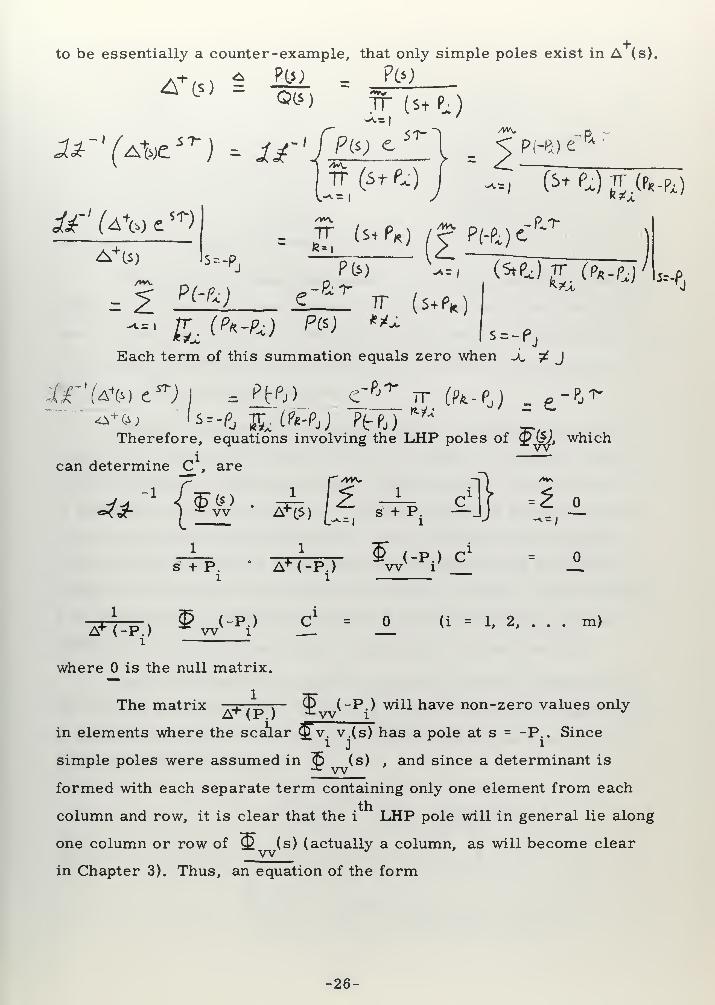
to be essentially a counter-example, that only simple poles exist in A (s).

A* CO =?0)

Qcs) jr (st ?:)

ST-

TT

TT (St Px.) V O k) ft^-Px)**,

A+CS) 's=-p,

/WV ft*

s=-PEach term of this summation equals zero when X. ^ J

jftr'teft) CD I = ftfj) e' ft^ TT (fa-PJ . „-6t-

Therefore, equations involving the LHP poles of £w, which

can determine C , are

s + P.1

A+ < -P.)f (-P.) Cw 1

*-fi

A+ , - , 5 (-p.) c]

A* (-P.) W ll

where is the null matrix.

1

(i = 1, 2, . . . m)

The matrix $ (~P.) will have non-zero values onlyA+(P.) j^vv i

in elements where the scalar OvTvJs) has a pole at s = -P.. Sincei ] i

simple poles were assumed in ^ (s) , and since a determinant is

formed with each separate term containing only one element from each

column and row, it is clear that the i LHP pole will in general lie along

one column or row of <£ (s) (actually a column, as will become clear

in Chapter 3). Thus, an equation of the form

26-

0>i o *

<Vo&

o

c

o oo

o

is patently not enough to determine _C .

Through the medium of an example involving a multi-dimensional

predictor, it has been demonstrated by counter-example that the proce-

dure of Hsieh and Leondes is not generally applicable. A method of un-

determined coefficients is only valid when it can be proven that the co-

efficients can in fact be determined.

15Amara approached the same problem, but attempted to find a

closed-form solution and was successful for a quite restricted class of

multi -dimensional random processes. Unfortunately, in his derivation

of the optimum system he chose to minimize instead of the mean square

error of each output the mean square value of the total sum of all the

errors, which could allow undesirable cancellation effects between the

individual errors and in general is not the best quadratic error criterion.

It is interesting to note that his implicit solution is identical with that

obtained by considering each error separately, as in section 2. 6.

Amara considered the class of random processes characterized

by a matrix of power density spectra, j£ (s), which can be transformed

to a diagonal form by pre- and post -multiplication by matrices with nu-

merical elements, such that

^w • u = d;,(s) /:,— — L ij rj J

where & is the Kronecker delta, (& = 0, i 4 i; &. - 1, i = i)ij ij iJ

£ (s)

w - u-1

rD..( S)i i [it]- 1

-27-

t +D. (s) = n.(-s) d:.(s)

Thus, the optimum system is given by

If [u J W (s) is considered as another optimum system, the

above equation in similar to n one-dimensional optimum systems, and

* - 1{[d{.(s)y [^]

- 1 w^)}& - i

fy^rQ v .i^W(>) = U

T

ifera ^>*_1

f6^=ar-rJ * !ii>

The requirement that the power density spectra matrix be diago-

nalized by a numerical matrix is a severe limitation on random processes

in general, as will become more clear in Chapter 3.

In summary, there is no hitherto published satisfactory solution

for the optimum n-dimensional system. The next section will consider

a more general approach to this problem, which will yield physical insight

into random processes and bypass the restrictions of the previously des-

cribed methods.

2.8 A new closed-form solution for an optimum multi-dimensional system

In the solution of the single -dimensional optimum system, where

from Equation 2. 14,

(d (s) was factored into RHP and LHP terms* w(jj (s) = (£""Vs) 5J

*(s) (2.25)= vv x w X w

and both sides of the equation were multiplied by -= j- . , maintainingx vv

-28

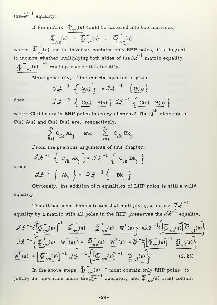
thecAZT equality.

If the matrix * (s). yy__ ~ w w

where $ (s) and its inverse contains only RHP poles, it is logicalwto inquire whether multiplying both sides of the J^F matrix equality

~m (s) would preserve this identity.

More generally, if the matrix equation is given

3&' 1 -[ms}} --A*~x

(b(s)}

does 1* _1{c(s) Ms)}-^-' 1

£.«.) BU)}

where C(s) has only RHP poles in every element? The ij elements of

C(s ) A(s) and C(s) B(s) are, respectively,

y C, Ak. and 5 C , Bk.

£1lk J kTi

lk J

From the previous arguments of this chapter,

*** { Ca^ } - 1*- 1

£ Cik

Bkj]

since

Obviously, the addition of n equalities of LHP poles is still a valid

equality.

Thus it has been demonstrated that multiplying a matrix UJf

equality by a matrix with all poles in the RHP preserves the <J<& equality.

***" 1

fe>>T ' ^w(s> O s) WT(s)j ^* '^[f^'g^U)

^"'($> »!«} |>> ^f) ^'{[f>>l"1

£££?}

WT (s> - [^>>] "* ^ "'{[f>>]"* fyM (2 - 26)

In the above steps, (£ (s) must contain only RHP poles, to

justify the operation under the,^- operator, and C£> (s) must contain

-29-

only LHP poles, to justify the removal of «/*" .

Further restrictions must obviously be placed on <P (s) and

$ (s). It has been shown in Section 2. 6 that 35 (s) = $" (-s)

Therefore, let $ (s) = G(-s) . GT (s) (2.27)

ww

where G(s) and G(s) are both physically realizeable. Thus

wx(s ) = fGT(B)]"

1

^"'{r^-fl)] i^<fl) "y < 2 - 28 >

In section 2. 5 it was pointed out that factoring the single dimen-

sional 2) (s) into tf) (-s) . 2T (s) determined w (s), the trans

-

fer function of a linear system which could reproduce the observed signals

when excited by white noise with unit power density. This is the Bode-4

Shannon approach . It is natural to inquire if a similar interpretation

can be placed on the factoring of (P (s).

Suppose a set of n uncorrelated unity white noise excitations, w.,•I

are applied to a physical matrix filter, G(s), as shown in Figure 2. 13.

W2

Ulto.

*- —>•

* —^.

t

•

1

Gcs) *

—>

IT

*̂v»

Figure 2. 13. A random process created by n white noise sources

V.(s) = Z_ G..(s) W,(s)J=i

ij J

/*- v^

£v v(s) = 2 G (-s) £ Gik

< s) ^ wl

but 3>w.w. = 1 1 = kIk= 1 / k

w.

•VU

^V. V.(S) = >1 J Js i

ll J 1/

5w

In matrix notation,

(s) = G(-s) GT(s) (2.27)

-30

which is the desired result. That is, the process of matrix factoring,

which leads to a closed-form solution to the optimum multi -dimensional

system, is identi cal to the problem of finding a physical system which

can produce the observed statistics with white noise excitation.

Thus, the multi -dimensional problem has been shown to parallel

exactly the single -dimensional case in notation and meaning, if the ma-

trix expression is substituted for the one -dimensional transfer function.

Chapter III will present various approaches and a complete solu-

tion to the formidable matrix factorization problem. It should be pointed

out again that this matrix approach produces the first general closed-form

solution to the optimum multi -dimensional system in the Wiener sense.

2.9 Statistical transformations on random vectors

A great similarity has been demonstrated between the scalar

and the matrix representation of random processes. For example, <£ (s)AA

describes a single random process just as $ (s) describes a set or

"vector" of n random processes. Some of the simpler relations to be18

derived were earlier presented by Summers , but in view of the sim-

plicity of derivation using equation 2. 9, they will be repeated here.

Consider first the simple configuration of Figure 2. 14

Figure 2. 14 X ~~r*~7* y

Multi -dimensional System

Y(s) G(s) X(s)j

Y.(s) = 2l G -(s) X(s >

J -Uvy^s) .j£ au<-.) £ G.

k(s) £ xlXk(s)

§ (s) = G(-s) $ (s) GT(s) (2.29)

yy xx

-31-

In the special case where x] is a set of uncorrelated white noise

signals with unit power density,

$" (s) = I-* YY —XX

£vvCS)= G( " S) G (S>

yy

verifying Equation 2.27.

^x y(s) = £ G (s) §x.xk(s)

J ±-j J

$_„_<s) = 1" (s) GT

(s)xy XX

Next, the summing operation of Figure 2. 15 is examined.

X —>- Gcsj

+i

)—*

y —> Hi*;

Figure 2. 15 A Multi -Dimensional Summing Operation

j-/ te=l

J-i k=/K

§> (s) = G<-s)<F(i> G(s) + G(-s) f (s) HT(s)

xyzz XX

+ H(-s) $ (s) GT(s) + H(-s) $ (s) HT(s)

yx yy(2.31)

The preceeding configurations were examined in deliberate

similarity to the scalar results of Section 2. 4. It inferentially appears

that a general formula for vector random processes can be expressed

just as Equation 2.9 applies to scalar processes.

-32-

A\» A&*

$" (s) = 2 ^-*--/ j^i

G.(-s) x. y.(s) H.' (s)J J

(2.32)

where the vector X( si =^ G.(s) X.(s) and Y(s7U Z H.(s) Y.(s) .

-k-I *•*< 1...

l Jth J >i _J J J

The ij subscript of 9P x. y.(s) refers to the i vector input, x. , makingIJJ— th

l

up x , and similarly for the j vector excitation of y „

To prove this formula, which is believed to be the most general

expression of statistical transformations in linear systems, consider the

system of Figure 2. 16.

L-Cs)

*»

x"-

>

• *

Xv,

G«,&)

MATRIX

G„<s)

H.(s)J

X.(s)i

Y(s)

X(s)

Y(s)

y,,

tt,(N

•

•

^, HjW \ +

*

ELEMI

Hja

2NT

G pq(s)

HJtu

(s)

X1(s)q

YJ(s)

u

X (s)P

Yt(s)

Figure 2. 16. A general multi-dimensional system/vu r

V s) =

1, (£GW 8>

•

x>>)

Yt(.) -

1 = 1

t h\u(s)

yJu(s))

From the basic equation, 2.9.

$ *^{s)- 1 C?(

GW- s))| {1,<^)K^

-33-

/*./fit-

1 ~2. G1(-s) "2. Hj

. (s) ^x^yj (s)

Li»i pl —-/tu q u J

2 Z. p Jt element oflG(-B) £ x

1y^s ) [hJ

(s)1

x(s) = ^ Z gV-s) £x* y

j(s ) [Hj(s)] (2.32)

-*=i J=-j

With the use of this formula, statistical relationships in multi-

dimensional system variables are swiftly expressed. An example will

prove the previous statement that Q .(s) is a sufficient description of—vl

the ideal signal in multi-dimensional optimization. Consider Figure 2. 17,

>fc G dcs;

+

w

1 -^5 v - W(?)e

^> XT —>

Figure 2. 17. Calculation of $ .(s)VI

where all variables are random vectors and all systems are matrix

operators.

= S(s)] + N(s)_

= [Gd(s>] s( S r

£L-(s) = 5L>> Ga(s) + ^ns(s) G

d(s)

v(s)

Ks)~

VI ss(2.33)

Thus, $ ,(s) is equivalent to Grf(s) if the input statistics are

known.

-34-

CHAPTER HI.

MATRIX FACTORIZATION

3. 1 Statement of the problem

This chapter is concerned with factoring a matrix of cross -power

spectra between signals in a multi -dimensional random process. Chapter

II has shown that solution of this problem will yield two significant results:

(1) A closed-form solution can be found for an optimum multi-

dimensional configuration in the Wiener sense.

(2) A multi -dimensional linear model is determined which can

reproduce the observed statistics when excited by a number of uncorre-

cted white noise sources.

The basic equation is

w3> (s) = G(=s) G (s) (2.27)

or, in expanded form,

Gn(-s)

G21

(-s)

Gnl

(- S )

v1v1(s)

^v^U)

ffv v (s)n 1

G12

(-s)

• •

• •

vlv2(s)

•Gm(

- S)

• •

• •

. . G (-sOnn

§ v^s)

v v (s)n n

Gn<s) G21

(s)

G12

(s) . • •

• • •

• •

Gi„<

s >

•Gm(s >

. . . G (s)nn

-35-

The G(s) which is found as a result of the factorization process

is the matrix filter described in (2) above. Each element of G(s) and

G(s) must be physically realizable in order to meet the requirements

given in section 2. 8 for the solution of an optimum multi -dimensional

configuration.

3. 2 Realizability considerations

Before plunging into a solution of this thorny problem, it is nee

essary and useful to examine the properties of W (s) which characterize

a set of random processes which could actually be found in the real world.

The ii element of $ (s) is Q)v.v.(s), where v. and v, are mem-

bers of an n-dimensional random process. Since $ v. v.(-s) = Q> v. v,(s),

| (-s) = f (s).^ w *• vv19

In addition, Kraus and Potzl have proven that a necessary

and sufficient condition for (p (s) to represent a valid multi-dimensionalT W

random process is that $ (jw) be positive definite for all co. This arises

quite naturally if the n signals are allowed to pass through a system G_

which multiplies each signal by an arbitrary constant and sums the total.

The power density spectrum in w of the single output is, from Eq. 2. 29,

G jfSjJ-)] g)

This spectrum must have a non-negative value for all values

of co, since a negative mean square value of power density cannot exist.

Thus $ (ico) must be non-negative definite for all values of co. Thevv •*

.

°

special case where IQ (joo) equals zero for all values of co will be con-

sidered separatedly in section 3.9, and a positive -definite limitation on

CD (j<*>) will henceforth be considered a valid demonstration of the rea-Wlizability of the random process. As will become more clear in the re-

mainder of this section, the only other case where a zero value of power

density can occur at a finite value of co is the occurrance of a multiple

even-order zero on the ju> axis in $ (s) .w

36-

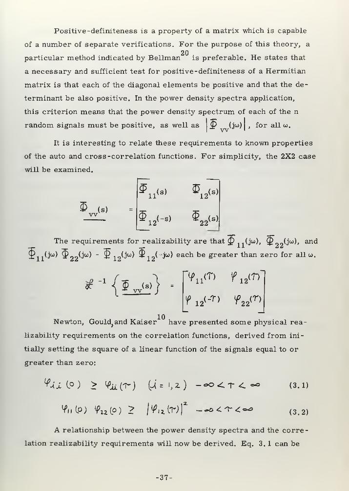
Positive -definiteness is a property of a matrix which is capable

of a number of separate verifications. For the purpose of this theory, a

20particular method indicated by Bellman is preferable. He states that

a necessary and sufficient test for positive -definiteness of a Hermitian

matrix is that each of the diagonal elements be positive and that the de-

terminant be also positive. In the power density spectra application,

this criterion means that the power density spectrum of each of the n

random signals must be positive, as well as Q (jco)w , for all oj.

It is interesting to relate these requirements to known properties

of the auto and cross -correlation functions. For simplicity, the 2X2 case

will be examined.

w(s)

*n<.> a>.12

(s)

12(~s)

22(s)

The requirements for realizability are that 

10Newton, Gould^and Kaiser have presented some physical rea-

lizability requirements on the correlation functions, derived from ini-

tially setting the square of a linear function of the signals equal to or

greater than zero:

^jlC°) > YjiCT-) (U=',2.) -<*0<T<L~" (3.1)

%L°) V>n(?) 2 |Valr;)x -*><t<~*

(3 . 2)

A relationship between the power density spectra and the corre-

lation realizability requirements will now be derived. Eq. 3. 1 can be

•37-

expressed for i = 1, as

4*ds $n(s)

" WT ds e ?u(s> - °2tTJ J -Tlr 27TJ

-J-° -J-*

Replacing s by jw,

-L-J

do (1 -eJwT^ ) 5U(J») >

joof*Since the real part of 1 - eJ is always equal to or greater than

zero, this integral will always be greater than zero if w^ Ajv>) > for

all oj. This relates the positiveness of (f (ju) (or $„ 2(jw) ) to the fact

that a signal has the highest correlation with itself as opposed to any

time -shifted version of itself.

At this point, it is well to ask if the positivity of ^L ..(s) can be

determined by inspection. It is not enough that ^ n1 (s) = ^^(-s). For

example, O^s) = . n . .-• ^r— satisfies this relationship but

_ r * 11 (-s+2) (s + 2)r

- ix> + 3 - r———

=

is negative for u> >J 3 t

u + 4

The example above contains a conjugate pair of zeroes on the jw

axis and is not factorable into ^ 1^s) . Q)

1..(-s). This pair of simple

zeroes are the only factors for which Q^ As) - $ . ^-s) and which cannot

be factored with mirror symmetry about the jco axis. Thus, factoriza^

tion is the only realizability requirement for a single power density spectra.

The second correlation function inequality, Eq. 3.2, maybe

written as

1J**,

ffiift) . JLy^ffu^) -

,>« loo

4 Jis, ^(Jje

S,r.

rJ-Hs1 c"

Sir^-Sv) >

-j-o

or, replacing s by jw,

-38

(a

The maximum value of eJ

1 ^2 3? io^I^ 12*"^ * wil1 occur

when cj = u = u and J) .. O(jto) is a maximum. Therefore, the minimum

value of the integrand is

$H<J»> f22(J«)-^ 2(-3«)5

ll.^)

for some value of w. If this integrand is positive for all w, which is the

previously given realizability criterion, the integral will always be pos-

itive. Positivity of this integrand is again equivalent to factorizability

of the 2X2JQ (s)

j, as was true for the auto -power density spectra.

In summary, the realizability criteria found in the literature for

the existance of the correlation and spectral functions of random processes

are related and the factorability of the individual power density spectra

and the matrix determinant is enough to satisfy all requirements. The

reason for the emphasis on this matter of realizability is that any method

of finding a real system which can create the observed statistics must

fail when either the diagonal elements or the determinant of (P (s)wcannot be factored, for otherwise the paradox of unrealizable signals

being created by a realizable system would exist.

3. 3 Two special cases

In this section, two special matrix configurations will be examined

which can be readily factored. These particular cases are of importance

since they provide goals for a more general factorization procedure.

When iP (s) is a diagonal matrix, each element must be able tovv

be factored into LHP and RHP terms, as shown in section 3.2. There-

fore,

3> (s) = D(-s) D(s)

39

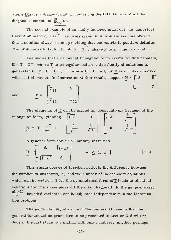
where D(s) is a diagonal matrix containing the LHP factors of all the

diagonal elements of 5 (s).

The second example of an easily factored matrix is the numerical21

Hermitian matrix. Lee has investigated this problem and has proved

that a solution always exists providing that the matrix is positive definite.

TThe problem is to factor H into X . X , where X is a numerical matrix.

Lee shows that a canonical triangular form exists for this problem,TH = T . T , where T is triangular and an entire family of solutions is

T T Tgenerated by T . U . U . T where U . U = I, or U is a unitary matrix

with real elements. In illustration of this result, suppose H =/ 1

3

5

and T =

11

12 22j

The elements of T can be solved for consecutively because of the

'^7TT

1triangular form, yielding

,TH = T . T

[7l3

5

13 TT3j

A general form for a 2X2 unitary matrix is

u = -l< <5L C

hfMT(3.3)

0.

This single degree of freedom reflects the difference between

the number of unknowns, 4, and the number of independent equations

which can be written, 3 (as the symmetrical form ofT leads to identical

equations for transpose pairs off the main diagonal). In the general case,

—-— bounded variables can be adjusted independently in the factoriza-

tion problem.

The particular significance of the numerical case is that the

general factorization procedure to be presented in section 3. 5 will re-

duce in the last stage to a matrix with only numbers. Another perhaps

-40-

more conceptual use of this special result is to visualize a matrix <P (jw)

as a Hermitian matrix which can be factored for every value of w, pro-

viding that the matrix remains positive definite (the realizability require-

ment), and thus a matrix which is some function of w does exist.

It might seem at first approach that a triangular form could be

postulated for ^ (s) factorization, in analogy to the numerical case.

This is unfortunately not true, as will be demonstrated below.

Referring to the general two-dimensional case,

£l2(- s) £ 22

(S)

Gll<->

LG <-) G22<-S)

G <.)

Gll<s) G

ll<s) = ^ 11

<S) = ^ ll(s> ^

+

ll4e>

Suppose that

Gn(s) = *>>

Gn(s) G21

(-s) = 5^-rt

G21

(S)" f

12(s)

Gn(-s)

G21

<S)

G22

(S)

If G. ,(s) has its zeroes in the LHP, G rt< (s) will have these as11 21

poles in the RHP. If G.js) had been selected to have RHP zeroes and-1

LHP poles, the inverse matrix G(s) would be physically unrealizable.

G(s)

Gn(s)

G21

(S)

Gu(s) G22

(s) G22

(S)

Accordingly, the triangular form does not yield both a solution

with a realizable and inverse realizable G(s). However, it offers a use-

•41-

ful method of reproducing a multi -dimensional random process in an analog

computer where inverse realizability is of no concern. To assure a rea-

lizable G(s) , the elements of which may be solved for successively, it is

only necessary to select the diagonal elements of G(s) with RHP zeroes

and LHP poles.

3.4 Properties of matrix transformations

The next section will present a general method for solving the

matrix problem

$ (s) = G(-s) . GT(s) (2.27)wThe philosophy of approach will be to multiply $ (s) by a suc-

cession of simple matrices, transforming it at every step, until the nu-

merical form is reached. In this section, the properties of simple ma-

trix transformations will be presented, emphasizing the viewpoint that

a matrix multiplication can be used as a tool to mold a given matrix

into a desired form.

There are three basic matrix manipulations to be considered:

(1) Multiplying a row by a function of s and adding it to another

row.

(2) Multiplying a row by a function of s.

(3) Exchanging rows.

In the above list and in the discussion to follow, operations on

rows by premultiplication are investigated. The results are equally

applicable to column operations through post -multiplication, however.

First, any row operation on a matrix can be accomplished by

premultiplying the matrix by an identity matrix on which the desired

row operations have been performed. The properties of interest in these

transformations include the value of the determinant of the transforming

identity matrix, and the realizability and inverse realizability of this

matrix. In this particular application, as will be shown in the next sec-

-42-

tion, row operations are performed with matrices whose elements must

have only RHP poles and whose inverse must also only have RHP pole

elements.

(1) Multiplying a row by a function of s and adding it to another row.

T(-s)

1

1

1

A(-s) B(-s) C( -s) 1

The above matrix multiplies the first row by A(-s), the second

row by B(-s), and the third row by C(-s), and adds the total to the last

|T(-s)| = 1.

-1

T(-s) 1

-A(-s) -B(-s)

1

-C(-s)

The simple form of the inverse will result for all matrices which

add to or from only one row. If A(-s), B(-s), and C(-s) have RHP poles

or no poles the matrices are proper for this application, regardless of

the location of the element zeroes.

(2) Multiplying a row by a function of s.

T(-s) =

1

D(-s)

The above matrix multiplies the last row by D(-s). T(s) = EX-s).

-43-

-11

T (-s) = 1

1

1

EX-s)

EK-s) must have both RHP poles and zeroes to be a proper trans

formation.

(3) Exchanging rows.

1

1

1

1

The above matrix exchanges the third and fourth row. IT I = -I.

= 1T = T.

The matrices described above perform simple transformations,

possess simple inverses, and in the second case can modify the deter-

minant of the transformed matrix by other than a constant.

3. 5 Matrix factorization: A general solution

A procedure is to be described in this section which will always

yield a solution to the matrix factorization problem regardless of order,

providing realizability criteria are satisfied. Because of the complexity

of the problem, no easy solution appears to exist. However, the method

of factorization to be presented here has been broken down into several

separate phases with each phase consisting of simple matrix transforma-

tions and each having a well-defined goal.

Each transformation step can be presented in the following fashion:

T.(-s) . $« . T.T(s) = I

1(S) < 3 - 4)

-44-

The relationship between the pre and post-multiplication matrice

is specified in order to ensure that (g (»s) = [(£> (s)J for all i.

The overall objective of this procedure is to produce a matrix

with numerical elements, 3^_ , after a number of successive transform

Aw

-*r Amations. Thus, if (p (s) = (J5°(s)

T^(-s) . . . . T2(-s) T^-s) §°(s) T^s) T^s) . ... Tr

T(s)

Tcan be factored into two numerical matrices, N . N #

Inverting,

^w(s) = g>°(s) = Tjf-s) . T2(-s) ...Tr^ g)

. NpT^s) . T2"(s) . . . Tr("s) .

j|T

" G<- s > •G T

(s>

G(s ) = T1

"<1-b) . T

2"(s ) . . . Tr"(s ) . JS (3,5)

G(~s} = N^1. T^(s) . . . T

2<s) . T^s) (3.6)

A proper solution of the problem will yield a physically-realizable

G(s ) and G(s) . This will obviously occur if T.(s) and T. (s) have LHP poles

only for all i. In other words, as (^ (s) is manipulated into various con-

figurations the realiz ability requirements on the solution will be met if

each transforming matrix meets these requirements. Drawing on the

results of section 3. 4, the following constraints exist on the elementary

matrix transformation T.(-s) :

i

(1) If T.(-s) multiplies one row of ^(s) with a function of s and

adds it to another, this function must have no poles in the LHP.

(2) If T.(-s) multiplies a row of ^ (s) with a function of s, this

function must have no poles, or zeroes in the LHP.

Since the equation

§\s) = T.(-s) ^(s) T.T(s)

is in the form of equation 2. 29, T.(s) can be interpreted as a physical

-45-

system with an input random process having a matrix of cross power

density spectra <5 (s), and with an output spectra of ^ (s) . The suc-

cession of matrix transformations then is equivalent to cascading a

series of physical systems until an output spectra involving only white

Tnoise -- the numerical matrix N . N_ - is achieved. This white noise

random process is operated on by N to produce a unit-valued uncorre-

cted set, whose spectra is given by the identity matrix. The total cascaded

system thus operates on the given random process and produces uncorre-

cted white noise, and is naturally envisioned as the inverse of the hypo-

thetical physical system creating the random process.

There are three general phases to this matrix factorization solu-

tion:

(1) Pole removal. The pole removal phase starts with the given

matrix and removes the poles of every element.

(2) Determinant reduction. The determinant reduction phase

converts a matrix with polynomial elements and with a determinant which

is also a polynomial in s, into another matrix which still has polynomial

elements but which has a unity determinant.

(3) Element order reduction. This phase operates on a matrix

of polynomial elements having a unit determinant until a numerical ma-

trix is reached.

To illustrate the central ideas of this method, a 2X2 example of a simple

yet non-trivial case of matrix factorization will be solved. Then, the

general case will be examined and each step justified.

EXAMPLE

Suppose a simple two-dimensional system is given by

1 1G(s)

+ 3

+ 1

+ 2

s + 4

-46-

and is excited by two uncorrelated unit -valued white noise sources. The

matrix of output power density spectra is

(£> (s) = GK-s) . G T(s) =

-isN II -Z5U+

(-Stl)(-S+H)(s-H)(5+3J (-*Hj(-5+4)(S+i)(*H)

The inverse of the matrix G(s) is

1 1

GKs)-1 (s+1) (s+2) (s+3) (s+4)

(- 4s + 10)

s+4

1

s+1

s+2

s+3 Jwhich is unstable or unrealizable. Thus, the question is posed: Can a

matrix G(s) be found which is realizable and inverse realizable, and is a

solution to

G(-s) G T(s) = $ (s) = <F°(s) ?w ~

(1) Pole removal phase

The objective of this phase is to remove all the poles in every

element. This is quite easily done by row and column multiplication.

T^-s)(-s+2) (-s+3)

(-s+1) (-s+4)

cg^s) = T^-a) (g^B) T*(b) = i~-2s2+ 13 - 2s

2+ 11

2s + 11 - 2s + 17

(2) Determinant reduction phase

In this phase we first desire to manipulate the^ matrix so it has

a determinant which is constant and independent of s. This will be the

-47

case if |T <-s)/

. I TT(s)

•<s)

Hence,

(s) - 16 s + 100 = (- 4s + 10) (4s + 10)

TiT2(-s) =

<£2(s) = T

2(-s) ^\s) T

2

T(s)

-4s+10j

- 2 s + 13

2s +11- 4s + 10

- 2 s + 11

4s + 10

- 2 s + 17

(-4s+10) (4s+10)

It is now desired to remove the poles in $ (s) without affecting

its determinant. An adding transformation is thus called for.

§ 2!<S>

=

- 2 s + 11

- 4s + 10.5s + 1.25

.375

=s + 2.5

— 2 kIf the first row of (j> (s) is multiplied by-

second row, the pole will be cancelled if

k . (- 2 s2+ 13)

s = 2.5

or k = . 75

The total added quantity will be

.75 , . 2. _ v . mM

s+2.5

+ .375

and added to the

375

-s+2.5 * "B r xi>/ - i. vMJ s T O. 1 ° ' -s + 2.5

T3(-s) =

r i

.751

-s+2.5

§3(s) = T

3(-s) l

2(s) t

3

TuI) =

- 2 s2+ 13

2 s + 5

- 2 s + 5

2

-48-

<|3<s) T

2(-s) . T

3(-s) <£

1

(s)J . TT(s

TT„(s)

-4s+10(-4s+10) (4s+10) .

4s+10

(3) Element order reduction phase

Consider the array of the highest-order powers of s in each3

element of ^ (s) :

-2s -2s

2 s

Note that the first row is equal to the second row multiplied by -s,

This is no accident, and arises because the determinant is independent

of s. Performing a reduction transformation,

T4(-s)

£4(s) = T

4(-s) . ^

3(s) . T

4

T(s) = 13

5

(4) Solution

This numerical matrix is, oddly enough, the example considered

in section 3. 3, for which the canonical triangular factorization is

N N(Hi

13

i

T^3

From equations 3. 5 and 3. 6,

G(s ) = T-_1

(s) . T2

=1(s) . T

3~\s) . T

4

_1(s) . N

GJs) = Nj1

. T4(s) . T

3(s) . T

2(s) . T^s)

-49-

GKs)

5s + 13 s

1(s+3) (s+2)

5s + 11

(s+3) (s+2)

s + 10fI3

(s+1) (s+4) (s+1) (s+4)

-1

G(s)52 (s+2. 5)

(s+10) (s+2) (s+3) - s (s+1) (s+4)

- (5s+ll) (s+2) (s+3) (5s+13) (s+1) (s+4)

This example has illustrated the significant features of the general

factorization procedure:

(1) Poles removed by row and column multiplications.

(2) Factors removed from a determinant of a polynomial matrix

through successive introduction and removal of the inverse factor as a

pole.

(3) Reduction of a unit-determinant polynomial matrix by operat-

ing on the highest powers of s in each element.

The general nxn case will now be examined.

(1) Pole removal phase

In the previous example, all RHP poles were identical in a single

row, and all LHP poles were identical in a single column. This configura-

tion facilitated the efficient removal of these poles by row or column mul-

tiplications, but did not occur coincidentally. In the general case the ij

element of $ (s) is G.(-s) G.(s) , where, G. (s), is the k row of G(s).w _|\ i t j_ J 1 k J

(s) will have the same RHP poles,All elements of the i row of w.th

which are the poles of G.(-s) , and the LHP poles in the i column of-xr Li I

© (s) will also be similar, except for occasional cancellation effects^ vv ^

in both cases.

-50-

(2) Determinant reduction phase

The resulting $(s) matrix, which has elements which are poly-

nomials is s, must have a factorable determinant with the RHP factors

a mirror image of the LHP factors about the jco axis. If not, the random

process is not realizable according to the discussion of section 3. 2. Con-

sidering the RHP factors, there is in general a constant and a number

of not necessarily distinct zeroes in this determinant.

Suppose that one determinant factor, -s + a, is selected. The

transformation matrix

T(-s)

-s+a

divides each element of the last row by -s + a. Let each of the resulting

last row terms be expanded by partial fractions. The residue of the pole

term in the nj element is ^ .(a). The important question now under

consideration is: Can each of the first n - 1 rows of Q(s) be multiplied

by a term i and added to the last row so as to eliminate simultane-

ously all•s+a

the poles in the last row?

thki ' ^ i

(a)

The added pole from the i row in the j column is-s+a

Accordingly, the equation to be solved for n - 1 values of k, is

/H-l

^ k £,.(a) = - <£ .(a) (j = 1, 2 .... n)

This in effect requires that the last row be a linear function of

the first n - 1 rows of (^(a). Since jQ) (a)| = 0, because - s + a is a

factor, the last row of(J)

(a) is always a function of at most the first

n - 1 rows and the above equations can always be solved.

The n - 1 element vector k. is found from>

•51-

£n-l< a) k]

I .(a))

n-1

of Q(a), and 3> .(a) contains the first n-1 elements of the n row of=5

—

nj J<E (a) .

where ^ .(a) is the square matrix of the first n-1 rows and columns"- 1 &

nThe pair of premultiplication transformation matrices is thus

OO

-

.

te*

r

P

o-S-f4_

O

o

fcl-l J-

O

*i *%> ' v' ^-

1

From a computational point of view, k should be determined

and first used to transform the polynomial matrix with the right hand nu-

merical matrix in the last expression above. Then, the - s + a factor

should be removed from each element in the last row by synthetic division.

The same transformation, only with the transposed LHP matrices

in post-multiplication, will remove the s + a term from ]$(s)L Thus, the

order of §5 (s) has been decreased by two. This procedure can obvious

ly be iterated for all factors, single or repeated, until the determinant

is only a positive constant K. Then, multiplying the last row and column

by|m will produce a matrix with polynomial elements in s and a unit

determinant.

The only case in which the procedure will not be applicable is when

the last row and column of $ (s) is zero except for the diagonal element.

But in this configuration, the diagonal element can always be factored

and the problem immediately degenerates to an n - 1 factorization prob-

lem.

52-

In summary, it has been demonstrated that a polynomial matrix

can always be reduced by simple transformations to a form which has

a unit determinant, independent of s„ This is an original contribution

to the general theory of matrices with algebraic elements, and is the

key to the solution of the matrix factorization problem.

(3) Element order reduction phase

The starting point of this phase is a matrix having a unit determi-

nant and the goal is to produce by successive transformations a numerical

matrix. An algebraic matrix having a constant determinant is called in

22the monumental work of Cullis ' an "impotent" matrix.

Cullis proves that any unit-determinant impotent matrix can be

obtained by successive multiplying-and-adding transformations on an

identity matrix. Since the inverse of these transformations always exist,

this means that there exists at least one set of transformation matrices

which can operate on the given impotent matrix to achieve the identity

matrix. Unfortunately, no method has been previously presented for

determining this sequence but the procedure to be given next appears to

be completely general and achieves the desired reduction.

Suppose an array is formed of the highest powered terms in s of

each element. Obviously, the terms in the determinantal expansion which

have the highest power of s will all be formed from these terms and must

sum to zero because the determinant is independent of s. In this array

identify the terms which make up the highest power of s in the determi-

nant. Replace the other terms in the array by zero. For example, suppose

the highest terms are

Is4 -2 s

33 s

2

Q 22 s -4s 6 s

2 23 s -6s -2 s

o

The highest power of s in the determinant is s . Replacing theo

terms not involved in the s term by zero,

53-

,4 n 3Is -2s

3 22 s -4s

-2 s2

The determinant of this matrix must be zero, so one row can al-

ways be expressed as a function of the other rows. In other words, a trans

formation can be readily found which will reduce the highest power of s

in the determinental expansion. In the above example, this transformation

is obviously performed by multiplying the second row by - -^-s and adding

it to the first row.

Iteration of this reduction of the highest ordered terms can be

continued until no element contains a power of s.

In the special case of the 2X2 impotent matrix, the determinant

of the highest powered terms of all four elements is always equal to zero,

and thus a series of simple operations of multiplying one row and adding

it to another will speedily reduce the 2X2 matrix to numerical form.

(4) Solution of the numerical matrix

The only requirement that a solution exist to the factoring of the

resulting numerical matrix is that it be positive definite. In the preceding

steps, the factorizability of the determinant was the only realizability

criterion needed. If one of the original diagonal elements had not been

factorable, this would not in general have impeded any of the steps up to

this point even though it would indicate an unrealizable system. However,

referring to the matrix factorization procedure as a succession of linear

systems operating on the random process, as was discussed in the be-

ginning of this section, it is obvious that "unrealizability" and "realiza-

bility" are both properties of a set of signals which are not affected by

passage through a linear system. Therefore, a positive definite numerical

matrix will result if the original power density spectra matrix satisfied

the realizability criteria. A non-positive definite matrix implies a set

-54-

of white noise having imaginary auto or cross correlation.

Appendix II gives a complete solution to a more complicated 3X3

factorization example.

Summary

This section has presented a general method for factoring a matrix

of power density spectra, providing that the statistics arise from a multi-

dimensional random process observable in the real world. Alternately, it

has been proven that a linear multi -terminal system, excited by white

noise, can always be found which (1) is stable, (2) has a stable inverse,

and (3) reproduces the observed statistical interrelationships in a random

process.

3. 6 Matrix factorization: An iterative solution

The method presented in the previous section is always valid, and

invariably leads to an answer which satisfies all requirements. This sec-

tion discusses an iterative procedure which will often yield a valid and

speedy solution without the need to determine and factor the determinant

of Q (s). This becomes especially valuable when the dimension of $ (s)

is high, and when digital computers are used.

The pole removal phase of the general procedure is readily accom-

plished, and the real factorization problem deals with the resulting ma-

trix with polynomial elements. Let this matrix be designated as Q (s),

which can be expressed as a power series in s with numerical matrix

coefficients

<5<s) = ^ sk

3? (3.7)

t-o

The problem considered is to find a matrix H(s) which satisfies

the equation

H(-s) . HT (s) = ^(s) (3.8)

-55-

where ,>n

- £H(s) = ^ s H (3.9)

T( S ) - ]2 <-l)

ksk H

k)f£sJ H T

H(-s) . H x(s)

I Z (-D s" H, ]| 2. sJ H.

>© -JEquating coefficients,

§> r = 2. ( = l)k H

k. H

r_ k(3.10)

/a —

where the range of k is bound by O fr ^ — /*v_ O £ f- k - /»\. .

The matrix factorization problem is, as an alternate interpreta-

tion, 2 m + 1 non-linear matrix equations. Suppose an approximate solu-

tion, H(s) , is known. If a small perturbation in H(s) is made with <JH(s)

and the resulting product is to equal (±) (s),

|r = 4 ("1)k

<Hk+ dH

k)(H

r- k+dH ,- k >

T

Neglecting the product <JHl . ct H as of second order, the

proper perturbation of H(s) is given by solution of the linear equations

Ir -f

t-0fc

Hk H^ £C-i)k{dHt H^ + «*^} (3.11)

The left-hand side of this equation is recognized as the matrix

coefficient of the f power of s in the error: <P (s ) - H(-s) . H (s) .

After these equations are solved for dH., the remaining f error will

be

^ dH • CJHT

* — £and the procedure may be iterated until the error becomes negligible,

providing that the original guess was "close enough".

Besides needing an approximate solution to commence this pro-

cedure, another drawback is that the resulting solution H(s) is not guar-

anteed to have a realizable inverse -- that is, H(s) may contain RHP

factors. To handle both of these requirements, a good initial solution

for H(s) will often be the LHP factors of the diagonal elements of $(s).

-56-

This first trial, while obviously in error if there are any non-zero off-

diagonal elements in $ (s), will be close to the solution if the cross-

correlation among the signals is weak. Also, it definitely has a deter-

minant which has all LHP factors, which a small perturbation in the co-

efficients of H(s) will not appreciably modify.

Having some promise of solving the matrix factorization prob-

lem with successive linear equations, it is useful to consider these equa-

tions in more detail. The set of equations to be solved is, from Eq. 3.11,

where ±— i|rs0 —-•

The new H(s) equals the original H(s ) plus dH(s) .

The total number of independent variables is the number of in-

dependent elements of <p. . For r even, where Q^. is symmetric, these

are the diagonal and above -diagonal elements. For r odd, where $ r is

skew-symmetric with zero-valued diagonal elements, these are the above-

diagonal elements. The total number of independent elements is thus

(m+ 1) (n) (n+ 1)|

(m)(n)(n - 1) _ (m , 1)n2 _ n<n I jj

The number of unknown variables is the number of coefficients

of cjH(s ), which is (m + l)n . Therefore, ~ elements of <jH(s)

can be arbitrarily selected, which reflects the degrees of freedom of

the imbedded numerical matrix in the complete rigorous solution. One

way of removing this excess is to specify that 4H be symmetric.

To illustrate these ideas and to indicate the expected degree of

convergence, the sample problem solved in section 3. 5 will be re-solved

iteratively.

After the pole removal phase,

-57-

£ (s)

- 2 s + 13

- 2 s + 11

- 2 s + 11

- 2 s + 17

The assumed solution for H(s ) is the LHP factors of the diagonal

elements of ^(s)

H(s)

1.414 s + 3.61

1.414 s + 4.12

H3.61

4.12H.

1.414

The equations to be solved are, from Eq. 3. 11,

<§e

= dH h|J+ H dHT

xo o '« o o

3Le

= dH H^ + H dH,'1 o 1 o 1

T TdH, H - H, dH

1 o 1 o

$ e

2

T TdH

lH

l "H

l 'dH

l

1.414

$G(s) =

- 2 s + 11

2 s + 11

As an example of the appearance of these equations,

sv gq ua 1*1!

L ii eg d^

dh

dh

12

22

3.61

+

4.12

3.61

4.12

dhn dh

dh

o

12Ct

22j

where dH was selected as symmetric. The boxed elements of .$ in-

dicate a set of independent equations. This set of equations can be solved

directly, yielding dh^ = 0, dh^ = 0, dh°2

= 1.424,

Solving the four remaining independent equations in <£.. , and ^„

yields

-58-

.660 s + 1.424

dH(s) =

.753s -I- 1.424

The new H(s) is thus

1.414 s + 3.61

.753 s + 1.424

.660 s + 1.424

1.414 s + 4. 12

H(-s)H(s) =- 2.435 s + 15.03

2 s + 11.02

- 2 s + 11.02

-,2.568 s + 18.93

lG(s)

.435 s - 2.03

- .02

- .02

+ .568 s - 1.93

Repeating the solution of the seven linear equations, the new H(s)

is given by

1.22 s + 3.285 .7456 s + 1.5348

.913 s + 1.5348

H(-s)H (s) = - 2.047 s + 13.15

1.128 s + 3.844

- 1.957 s - .012 s -I- 10.95

- 1.957 s2t .012 s + 10.95 -2.105 s

2+ 17.16

which is compared with the actual <]5(s)

<§ (s> =- 2 s + 13

2 s + 11

-2s +11

2 s + 17

This solution is probably within the accuracy of measurement

of 4>(s), and no further iteration is made.|h(s)

|

= .697 s + 5.862 s +

10. 66 which is stable.

-59-

In high order problems evaluating and factoring the determinant

of H(s) can be a very difficult step. If an indication of inverse realiza-

bility is desired, an approach similar to that used by the Nyquist stability

criterion is very useful. i , . > i is evaluated, possibly by a digital

computer, for a sequence of various values of oo and plotted on a complex

plane. The presence of RHP factors will then be detected by any net num-

ber of encirclements of the origin.

To summarize, the described iterative method presents an attractive

alternative to the complete factorization procedure, especially when digital

computation is employed. In an example of this method, two iterations

solved the problem to an acceptable accuracy level. The price which must

be paid for this computational advantage is the possibility of a non-con-

verging solution or one which converges on a solution having an unrealiz-

able inverse.

3. 7 Matrix factorization: A lightning solution

This section considers a very special case of matrix factorization,

but one which is quite simple to solve. The central requirement is that

Teach non-zero element of any single row of G(s) , where G(°s ) . G (s) =

<3? (s), must have separate and distinct poles and must have a deno-

minator of higher order than the numerator.

The ijt

off-diagonal element of ^ (s) is £ G ( -s) &-y &) « **J

t

5 )

Q^O)The first question to be considered is whether each of the n terms

p ( s )G (-s) G (s) can be recovered from a knowledge of ii_ . Alter-

P (s) q ( s )nately, if a partial fraction of ij is made, ij can all

~Q (s) Tpoles belonging to a single ij

k

element of G(-s) or G (s) be

grouped together, and can these groups be further separated into LHP -RHP

product pairs ?

The key to this grouping is that any scalar function A(-s) B(s),

where A(=s) and B(s) have RHP and LHP poles respectively, has an in-

-60-

verse time-domain transform fU /which is continuous across the origin

as long as the order of the denominator is at least two degrees higher

than that of the numerator of A(-s) B(s). This can be proven by showing

that f(0 ) = f(0 ) which, by using the contour integral to sum residues,

becomes

—^r- ds A(-s)B(s) = -£-, (dsA(s)B(-s)27TJ J 27TJ J

The latter equation is valid since the right hand side is merely the

left-hand side with the sign of the integrating variable changed, as the

negative sign of the differential is cancelled by the limit exchange.

As an example, let

A(-s) B(s) =(= s + 7) (s + 2) (s + 4)

f<r> ' T3

vre

1

6

- 2Te

f(o ") = f(o+

)

1

22

- 4Te (no)

Thus, the residue of the LHP poles must sum to those of the RHP

poles in the partial fraction expansion of any such function as A(-s) B(s).

P..(s)

Therefore, the partial fraction expansion of \ . can be grouped

to show this residue equality between, in general, n sets of LHP and RHP

poles, providing that all elements have distinct poles. If i = j, each LHP

pole has an equal RHP pole in the partial fraction expansion, and this

grouping is impossible.

Suppose that n such sets of RHP poles have been determined in

one element of the first row of y? (s). Under the assumptions of thevv F

form of CKs), these sets should satisfy residue equality requirements

in every off-diagonal element of the first row of Q (s). The first diagonal

element is similarly grouped, and the corresponding LHP and RHP terms

61-

of each set are multiplied together. The resulting n terms are ^^(s) =

^ £*A~5)G. .(s), and thus when individually factored, yield the first row

of G(s) which may be placed in any desired order.

Having fixed the first row of G(-s), given byGJ-s), the j element

of the first row of 3>* (s) is.G.(-s) . G.(s) , and thus G.(s) can be foundw ) 1 I J J J

directly for all j, since the residue equality requirement associates each

element ofG.(s) with the known set of poles in an element of,G,(-s),

T U I

L-J f

G(-s ) G (s ) is then evaluated, and under the restrictions of distinct poles

ofG(s), will equal CE (s).wAs an example, the much -battered veteran of this chapter will

be resolved.

$ (s) =w- 2 s

2-I- 13 - 2 s

2+ 11

h

(~s+2) (-s+3) (s+2) (s+3) (-s+2) (-s+3) (s+1) (s+4)

- 2 s2+ 11 - 2 s

2+ 17

(-s+1) (-s+4) (s+2) (s+3) (-s+1) (-s+4) (s+1) (s+4)

2<5 , .

- 2 s" + 11x v,v.Xs) =rr ' ( -s+2) ( -s+3) (s+1) (s+4)

-s+2 -s+3 s+1 s+4

(-s+3) (s+1) (-s+2) (s+4)

The poles at s = 3 and s = 2 satisfy separate residue equality

requirements, lending support to the hope that $ (s) can result from a

G(s) with distinct elements.

^t

. - 2 s2+ 13 1 1

VlVr S

' (-s+2) (~s+3) (s+2) (s+3) (-s+3) (s+3) (-s+2) (s+2)

LetG,,(-s) =*

and G,J-s) =11 ' -s+3 12 -s+2

I v^s) = Gu(-s) G21

(s) + G12

(-s) G22

(s)

-62

G„,(s) = —^t G^Js) =21 s+1 22 s+4

and the resulting G(s) is given by

GKs) = s+3 s+2

s+1 s+4

and GK-s) G (s) yields the given $ (s)„wBut the problem is not yet complete, and this example was pur-

posely chosen to illustrate a significant defect of this simplified attack.

As given in section 3. 5, G(s) contains a RHP pole and is unrealizable.

Generally, the resulting solution in this method may or may not be in-

verse realizable, but its simplicity makes the attempt worthwhile as a

preliminary to the increasing rigor, generality, and computational

complexity of the methods given in sections 3. 6 and 3.5.

3.8 Statistical degrees of freedom of a multi -dimensional random process

Up to this point it has been assumed that $> (s) is a non-singular

nxn matrix. If 5^ (s) = 0, this implies that one or more rows of a

hypothesized nxn G(s) is a linear function (not necessarily numerical)th •*£:

of the remaining rows. Suppose the k row of G(s),{

G, (s) = ^. C.(s) •

|G.(s) (k>/n). v (s) = |G (s) W(sW , where W(s)J is the hypothe-

sized transform of the white noise excitation vector over a finite interval.

^-i -«•-/

Therefore, v, (s) is a redundant member of the set of signals and

can contribute no additional statistical information on the multi -variable

random process. At this point the representation of G(s) as an nxn matrix

excited by n uncorrelated white noise sources is open to question, since

there are less than n "useful" outputs.

-63-

Suppose, by striking out pairs of rows and columns, the highest

order non-singular matrix contained in (s) is found. Denote this raa-

trix as CP (s), representing a set of m independent components of themset v. It has been shown in this chapter that if physical realizability

criteria are satisfied (s) can be factored into G (-s) . G (s), with G (s)^m m m mexcited by m white noise sources. It appears logical that the remaining

n - m dependent signals can be derived from these m white noise sources,

as shown in Figure 3.1.

Figure 3. 1. Formation of a multi-dimensional random processwith redundant elements.

The adequacy of this model will be proved in the following steps:

a H (s) will be found which satisfies the cross power density spectra

relationship between every v. and v.. It will then be shown that this H (s)k l n-m

produces signals v which have the proper cross power density spectra

among themselves. Thus every signal will be related as indicated in the

original $ (s) matrix and Fig. 3. 1 will indeed be a valid representa-

tion of a multi -dimensional random process with a matrix Q (s) of

rank m."W

To better picture the following steps, Q^^(s) is shown in parti-

tioned form.vv

-64-

J

I

l&I CO I *w* J

(3.15)

From Eq. 2.32,

$v.vk(s) = G_(-s) H]~_(s)m n-m

H J" (s) = G~'(-s) 3?v.v.(s)n-m m -^ 1 k(3.14)

[G (-s) exists because of its non-singularity. But also, H (s) mustm -i' n-m

satisfy the equality.

v. v (s) = H (-s) . H (s)k k n-m n-m

From Eq. 3. 14, the following relations must hold for the parti

tioned sub-matrices of Cp (s)w

^Vk(s) £Vk<- S> [

Gm" 1(s)]T

- [O^l- ^Vk< s)

= I <•) <£ m" 1

(s) $ v.vk(s) (3.15)

Since <E7 (s) is of rank m, each of the last n-m rows can be

considered as a linear function of the first m rows. Let ,$. (s) = ^. A. .(s)-. \ JL I -1=1 «i

.$ .(s) where <j>, (s) and <F.(s) are row vectors of ® (s) and A, .(s)I i

| L k t i i | w ki

is a scalar to be determined. Writing this equation in complete matrix

form, and recognizing the resulting partitioned matrices,

[ VlWJ $vkvk<s)] - [A(s)][$ m(s)!^v.vk(s)]

^v.v.(s) = A(s) <g_(s)k l m

and ^v.v.(s) = A(s) ^v.v.(s)k k i k

x

A(s) = §v,v.(b) m _1(s)

k l * m

-65-

$Vk<s) = ^V v.( S ) $

k i m (s) i v .i\(s)

Thus equation 3. 15 is verified, providing that some matrix A(s)

exists, and the assumed form for H (s) produces the observed sta=n-m r

tistics. Note that H_ _(s) is fixed for a choice of G__(s) . Transposingn-m m

Eq. 3.14,

H (s) =n-m ^V.V.(-B) [G^-S)"]

k l L. m -1

A(-s) 3> <-s) rG^-s?1

m L m J

A(-s) G (s) GT(-s) [GT(-s)lm m L m J

-1

A(-s) Gm(s) (3.16)

For H (s) to be physically realizable, A(s) must contain only RHP

poles. A(s) was used as a row transformation to express the redundant

rows as a function of the independent rows. The elements of A(s) can be

used in an elementary transformation at the beginning of the factoriza-

tion problem to eliminate all redundant rows and columns, leaving $> (s),

Physically, this means that the random process v is passed through a

matrix filter B(s) , such that the resulting output power density spectra

matrix

= B(-s) $ (s) B 1(s)w m

where B(-s) = II

-A(s)|

I

That is, B(s) weights and adds together the m independent signals

of v and nulls out the redundant signals. As discussed in the first para-

graph of this section, this dependence among signals, if observed in a

stable random process, must arise in a physically realizable system.

Therefore, B(s), containing all the elements of A(-s), must be physically

66-

realizable or ^ (s) does not represent a real process.

Thus an index of randomness of a multi -dimensional random

process is the rank of the matrix of cross -spectra or, alternately, the

number of white noise sources needed to reproduce the statistics of the

process. Also, a set of dependent random processes is physically rea-

lizable only if the redundant rows of the matrix of power density spectra

can be removed by a row transformation with RHP pole factors.

-67-

CHAPTER IV.

NEW RESULTS IN OPTIMUM SYSTEM THEORY

4. 1 Introduction

The previous chapters have been in a sense an introduction, although

a useful one, to the main theme of this report. It has been demonstrated

that a linear system excited by white noise can always be found to dupli-

cate the basic statistical properties of any stationary random process,

single or multi- dimensional.

In standard texts on random processes it is customary to note

that a power density spectrum has the same form as the spectrum of the

output of a linear filter excited by white noise. In the early paper by Bode4

and Shannon , which served to convert the highly mathematical approach

of Wiener into a form more understandable to engineers, this white noise

filter and its inverse were used as a means to remove all memory from

the random process and to justify the use of a straight<3^- operation to

obtain the optimum configuration. In this work the idea is carried one

step further and the hypothesis is offered that within the confines of a

linear theory a random process should be viewed as actually being the

result of white noise exciting a linear system. Although this system in

some cases cannot be physically represented and the white noise sources

cannot be traced to microscopic random phenomena, it is possible to

make measurements on the random process itself with complete mathe-

matical assurance that there is such a linear system "upstream and

around the bend".

This hypothesis would be only of mild interest by itself, but this

chapter will show how this simple assumption makes the study of sta-

tionary random processes purely a measurement problem and how it tends

to unify the conventional analysis techniques of linear systems and those

of stochastic processes.

68-

4. 2 Matrix differential equations and system state

The heart of the description of a linear physical system is its

"state", which effectively describes the condition of every internal en-

ergy storage element at every instant. Since a random process is to be

analyzed in terms of its equivalent system, it is useful at this point to

summarize the major features of the matrix theory of differential equa-20

tions, such as is found in Bellman , in order to emphasize the state

approach to the analysis of linear systems. In this case, matrices allow

compact expression of ideas without regard to order and dimensionality

of the system under consideration. The standard theory outlined in this

section will provide a foundation for clear presentation of the original

results to be presented in the remainder of this report.

The basic matrix representation for a linear system is presented

in the following equation

d

dtx = A x + D u (4.1)

where x is the n-dimensional state vector of a linear system, A is a

constant nxn matrix, D is a constant nxm matrix, and u is the m -dimen-

sional excitation vector. For example, consider the simple second-order

system of Figure 4. 1, where a spring-mass -dashpot system is being ex-

cited by an external force F.

B -n

X

MK

Fig. 4. 1 A simple second-order system

Here the differential equation is

M 4*X +d* ;

B d* +~33r

Kx = F

dxDefining one state variable, x to be x, and x_ to be is

sufficient to fix the potential and kinetic energy of the system. The sys

tern equations are next cast into the general form of Eq. 4. 1.

-69

d -htl

The initial condition response or free behavior of linear systems

will be of particular importance in the study of random processes in

following sections. Given x (0), it is desired to find x (t) under condi-

tions of no external excitation. It would obviously be desirable to have

a solution in the form

x (t) = B (t) x (0)

Assuming this form and substituting into Eq. 4.1,

B (t) x (0) = A B (t) x (0)dt

or

The series

_d_

dtB(t) A B (t)

2 t

wheredt

B (t) = I + At + A yB (t) = A + A2

t . . . . + An

+ An t

n

n-1

(n-1)!

n!

= A B(t)

satisfies this equality.

Thus,

B(t)

-on t

n

A —; , where A° =• Lis the desired

*a = o n 1

'

Atsolution and is known as the matrix exponential e , a quantity that is

convergent for any value of A and t. It is analogous to the scalar ex-

ponential, and occupies a position of pivotal importance in linear systems

analysis.

If Eq. 4. 1 is Laplace transformed,

s x(s) - x (0) = A x (s) + D u (s)

x (s) = [si- A"!_1

x (0) + [si- A"]"1D u(s)

(4.2)

-70

The eigenvalues of the matrix A are thus the pole locations of

the transform of the transient response. If, for example, A has only

diagonal elements A •>

[--r = [t^-\x.(0)

and x.(s) = r

—

1 S -A.

x.(t) = x.(0) e^1(4.3)

1 l

In this case, the state variables refer to a system which, in La-

place transform terms, has been expanded by partial fractions into a

series of simple poles. There is no unique state of a system, since any

non-singular linear transformation can be made on a particular set of x.

If x = T y, substituting in Eq. 4. 1 yields

t|- y - ATy

ar y = T"lAT y

A transformation on A, where T AT becomes a diagonal ma-20

trix, is always possible if A has distinct eigenvalues . In this case,

the general solution for a free system is, from Eq. 4. 3

y(t) = [e^ £ y(0)

T_1

x(t) = [e^ cf. . T"1x(0)

rl

x(t) = T [e^ <T..l T"1

x(0)

Therefore,

eAt _ T rVr] f l

for any A which has distinct eigenvalues X. and which is reduced to diag-

onal form by T. In the general case, from Eq. 4. 2

eAt

- i- 1 [si -A]" 1(4.4)

An alternate way to visualize the concept of state is to integrate

and Laplace transform the basic equation, Eq. 4.1, yielding

= 71-

x(s) = — x(0) + — Ax(s) + — D u(s) (4.5)s s s

This expression with integrals immediately yields a form suitable

for direct mechanization on an analog computer. The number of integrators

required would equal the dimension of x. The input to the ith integrator

would be /yv *v

j-i j«i

and its output would be the ith state variable of the system x.(s). Relating

a state to an output of an integrator lends a particularly clear meaning to

this concept.

In summary, the state of a system is the set of numbers which at

every instant is sufficient to define the signal level in every energy storage

element. In a linear system which is not externally driven, the state tra-

jectory is given by

x(t) = eAt

x(0) (4.6)

4. 3 Interpretation of the optimum linear predictor

The mathematical form for a linear predictor, optimum in the

mean square sense, was one of the first significant results in random1 2

process theory, as presented by Wiener and Kolmogorov . This section

will show that this predictor has a very simple interpretation in terms of

the generating model for the process. For generality, the multi -dimen-

sional case will be discussed, which of course includes the scalar or lxl

problem.

Chapter 3 has shown that a random process can always be viewed

as a generating matrix G(s) , excited by a set of unit-valued uncorrelated

white noise spectra. The optimum predictor for T seconds in the future

in a random process is given by

WT(s)

[gt(s) j"

1

jy "V g'Vb ) £vi

(s)\ (2 - 28)

-72 =

where

Iv.<s) - I vv

e I

q'K Te G(-s) G (s)

After transposing, and substituting in Eq. 2. 28

W (s) *4£ -ie87"

G(s) G_1

(s)

(2.33)

(4.7)

Figure 4. 2 shows the resulting structure. The input white noise

vector w is successively transformed into the given random process v,

*><*)Gcs) > G(s)~

w#;^-'{e sr

^j}v (£+?-)

Fig. 4. 2 Configuration of an optimum multi -dimensional predictor

back to the original white noise, which then passes through a system

given by^ |eS

G(s) y .

Suppose first, for simplicity, that the ijth element of G(s) con-

tains only simple poles.AY\s

Gy(S)k.

A*-\ s + a.

This element can be portrayed in flow graph form, as shown in

Figure 4. 3.

/MPUTOUTPUT

V;

Fig. 4. 3 Typical transmissions of the ijth element of G(s).

The set of values for x. completely defines the state of the system

and if white noise excitation should suddenly be cut off at t = 0, x.(t)

-a«t1

would equal x.(0) e *•.

l

The ijth element of J.& \e G(s ) r is then

-^r

-= / 5 + A.X S+ Au

-73 =

A flow graph of this system is given in Figure 4. 4.

-o.,r

OJTPuT

ITji (Jt+T)

Fig. 4.4 The ijth element of jfof ]_ eS

G(s)[

A very significant interpretation can be made from comparison

of Fig. 4.3 and Fig. 4.4. G..(s) and fy <e G..(s)V have the same

excitation, and continually reproduce the same state variables, x.. The

difference is that the output from each first-order system which helps

to form the prediction for v.(t +T) is weighted by the value of the unit

initial condition response in fof its own system. That is, just as the

present value of v. is a linear numerical function of the state variables,

so is the optimum predictor the same linear function of these state var-

iables after an initial condition decay of T" seconds.

More generally, the best prediction in a mean-square sense of

the state of the random process T seconds in the future is the initial

condition response of the generating system from this state. Upon re-

flection, this seems to be a reasonable result when one views the state

at time t +T as the sum of the initial condition response from the state

at time t and the results of white noise excitation from time t to t +T,

the latter being essentially a zero-mean unknowable response.

The above demonstration included only the case of simple poles.

As G..(s) may contain multiple-poles, it is necessary to verify the decay

of the state as contributing to the optimum predictor for this case. In

all of linear transient analysis, the case of multiple poles is one handled

with considerable difficulty. In the following proof, a canonic flow-graph

= 74-

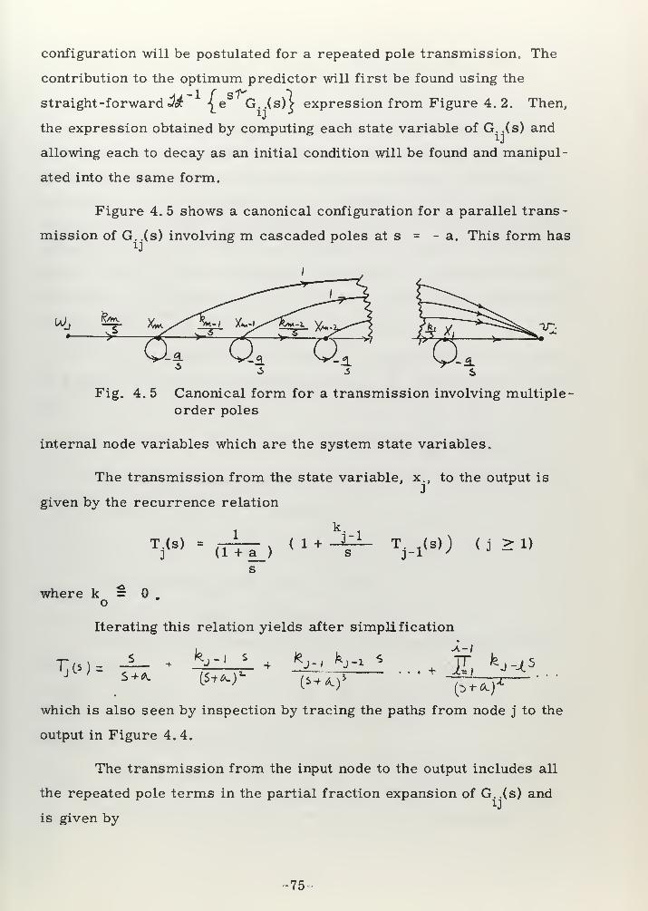
configuration will be postulated for a repeated pole transmission. The

contribution to the optimum predictor will first be found using the

straight -forward J& 4e G..(s)> expression from Figure 4. 2. Then,I

the expression obtained by computing each state variable of G..(s) and•J

allowing each to decay as an initial condition will be found and manipul-

ated into the same form.

Figure 4. 5 shows a canonical configuration for a parallel trans-

mission of G..(s) involving m cascaded poles at s = - a. This form has

ujj a*

Fig. 4. 5 Canonical form for a transmission involving multiple

-

order poles

internal node variables which are the system state variables.

The transmission from the state variable, x., to the output is

given by the recurrence relation

V s> =(TTT) <1+ ^r- T

j-i(s)

) <J ^ x)

where k =• .o

Iterating this relation yields after simplification

T>) =S + A.

Jy s+ *,-. fej-i

l ... +jr kJrl

(s+*ofc

0+*0 :

(F^Fwhich is also seen by inspection by tracing the paths from node j to the

output in Figure 4. 4.

The transmission from the input node to the output includes all

Bate

is given by

the repeated pole terms in the partial fraction expansion of G. .(s) and

75

(St-*.)**'

It is hypothesized that the contribution of this repeated pole

transmission of G..(s) to the optimum prediction of the ith variable is

given by the sum of each of its state variables allowed to decay as ini-

tial conditions for T seconds. Thus the cascaded system of Figure 4, 2,

which operates on the "recovered" white noise w., should supply a trans-

mission from w. to the T node, x y , weight by the numerical factor of

the unit initial condition response in f from node r, and sum over all r.

This system must then be equivalent to the result of applying the known

solution^ I e G..(s)V for this multi-pole leg.

The unit initial condition response L-(s) from node r to output v.rt

i1

of Figure 4. 4 is given by applying a unit step, —, to the rth node, yield-

ing

!>&) = -i- T>(s; -

The inverse Laplace transform of I (s) is the desired weighting

for the rth state variable as a function ofT.

The transmission from input to node r is

Therefore, the repeated pole part of the hypothesized optimum

predictor is

~ X^ (t"*r *2 1, *^ T-d-*r l (4.8)

which should equal the known result J_

The similarity in these two expressions is not staggering. The

= 76-

quantity^ j e T. (s) i- will now be manipulated into the form of Eq. 4.8,

-4. ;

r *

{

£9 iL k^ z-* * (j)^'J rJ e_

^}

where ( . ) is the binomial coefficient,3 ™ ™2 ™ ' (i - j) S j !

Expressing this series in terms of powers of where j = i-p

^ = o ^A L-taf (X-f) j

J

Replacing i by m-r+u and p by m-r,

^ ts+A)**— 1

T^ A *u-< r e'

tf]

(S+A.)'

which is equivalent to Eq. 4. 8, completing the proof.

A more elegant proof can be made with the aid of relations de-

veloped in Section 4. 2, where G(s) is considered a general system with a

set of state variables, x, described by the matrix differential equation

~- x = A x + D w (4.1)dt

and where the output v is given by v = R x.

From Eq. 4. 2, the input to output transfer function is implicitly

given by

v = R [[sI-Al" 1 DwIt is desired to prove that

-77-

d* - 1{e

S^R [s I - A]"1 d} = R e^fsI-A]" 1 D

which means that w is operated on by [s I - A^j D to produce the current

state variable vector, x(s), which is then weighted by its initial condition

ATdecay e and reproduced at the output by R.

^{e^R Csl-A]- 1 D]= ^ { R eA(t+r) D }

= S {ReAr eAt D}

20according to a property of the matrix exponential proved by Bellman

And, completing the proof, which applies for single and multiple

roots alike in single and multi-dimensional systems,

X{R eAr

eAt D} = R e^ [s I - A^"

1 D

In sharp contrast to the arduous multiple -pole derivation made

above with involved manipulations with series, the use of the general

state equation provided the desired results with a minimum of effort.

Thus it has been proven that the optimum linear predictor for a

stationary random process can be regarded in all cases as the result of

computing the state of the random process and allowing these state

variables to decay as initial conditions in the given model of the process.

The significant feature of a random process is then its state,

which summarizes for use in the present and for future prediction all

past behavior of the random signal or signals, using a compact number

of variables. An expected trajectory of the state variables of the random

process, and any system on which it may act, is then defined at every

instant by these state variables just as a free determinate system settling

to equilibrium is defined by its state variables at a single instant. This

allows a wealth of known information concerning the behavior of unforced

linear systems to become applicable to systems which are driven by ran-

dom processes, especially in control applications. Chapter 5 will ela-

borate on this interesting by-product of the new approach to the repre-

-78

sentation of random processes by the state concept.

The concept of state is only useful if the state variables are re-

coverable from operations on the random process alone. If the matrix

model, G(s), has a realizable inverse, which accounted for most of the

difficulty of Chapter 3, this is obviously necessary and sufficient in

order to ensure that the state variables can be separately found by a

stable system.

Having found that the future value of a random process is given

by (1) the sum of present state values decaying as initial conditions, and

(2) the response of an "empty" system to future values of white noise, it

is now interesting to investigate the knowable properties of this white

noise buildup.

The error of the optimum single -dimensional predictor will be

solely due to future white noise excitation. Figure 4. 6 shows this optimum

configuration.

uJ

Oris)ir

G-C5)^-^"'{€ sr

^;} {

-h esr

Xg)—•*£

Fig. 4. 6 Error configuration for an optimum single -dimensional

predictor

The transmission from w to e is

H(s) = G(s) e3^ -M " 1 {eSr (3(s)]

Suppose that the impulse response of G(s) is w(t).

H(s) = eSr

w(t) e~ St

dt

f t

3> (s) - H(s) H(-s) = wUJ e"S

1 dt1ee J 1 1

i~o -T Tw(t

2) e

St2 dt

2

1 s(t -tj

assuming that the order of the integrations may be changed. But

-79-

rJO°

35 Jds e

S<VV - ^ D (t2

- £,)

-Joo

where >U.(t) is the unit impulse at t = 0.

2e (r) = J dtj w^)

Jdt

2w(t

2) ^(tj-tj)

o

-r2

eIT) = J dt w (t) (4.9)

o

This general result indicates that the mean-square value of signal

level at the output of a linear system, when the white noise is suddenly

turned on at t = 0, is equal to the integral of the square of the impulse

response from the excitation point to the output. As a check,

e2(^o)

J

dt w2(t) = -£ I

ds G(-s) G(s)

ds $ (s) = V2

w2*j

Obviously, if more than one uncorrelated white noise source is

driving a system, the resulting variance of an output signal is equal to

the sum of the variances from each excitation point considered separate-

ly. The next section will use this result to motivate a quantitative replace-

ment for the Nyquist sampling theorem.*

4. 4 A quantitative measure of sampling error for non-bandwidth limited signals

A classic problem in numerical analysis, pulse code modulation,

and sampled-data control systems is the loss of information because of

representing a continuous signal by a series of evenly-spaced samples.

The conventional approach is to utilize the so-called Nyquist Sampling23

Theorem as given, for example, by Ragazinni and Franklin , which

states in essence that a signal of absolute bandwidth J[ can be recovered

if T, the sampling interval, is less than —~— .

In practice, since absolutely bandwidth -limited signals do not occur

=80

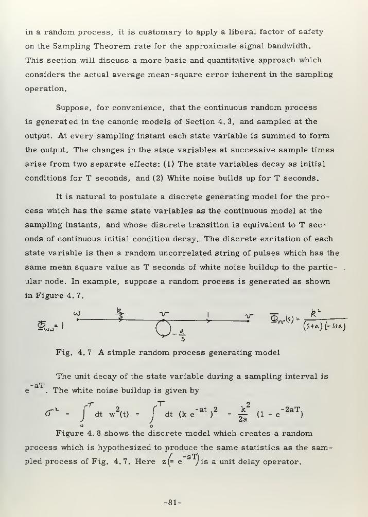
in a random process, it is customary to apply a liberal factor of safety

on the Sampling Theorem rate for the approximate signal bandwidth.

This section will discuss a more basic and quantitative approach which

considers the actual average mean-square error inherent in the sampling

operation.

Suppose, for convenience, that the continuous random process

is generated in the canonic models of Section 4. 3, and sampled at the

output. At every sampling instant each state variable is summed to form

the output. The changes in the state variables at successive sample times

arise from two separate effects: (1) The state variables decay as initial

conditions for T seconds, and (2) White noise builds up for T seconds.

It is natural to postulate a discrete generating model for the pro-

cess which has the same state variables as the continuous model at the

sampling instants, and whose discrete transition is equivalent to T sec-

onds of continuous initial condition decay. The discrete excitation of each

state variable is then a random uncorrelated string of pulses which has the

same mean square value as T seconds of white noise buildup to the partic- .

ular node. In example, suppose a random process is generated as shown

in Figure 4. 7.

Fig. 4.7 A simple random process generating model

The unit decay of the state variable during a sampling interval is

-aTe . The white noise buildup is given by

=J

dt w (t) = I dt (k e ) = — (1 - e )

Figure 4. 8 shows the discrete model which creates a random

process which is hypothesized to produce the same statistics as the sam-

pled process of Fig. 4. 7. Here z(= e J is a unit delay operator.

-81

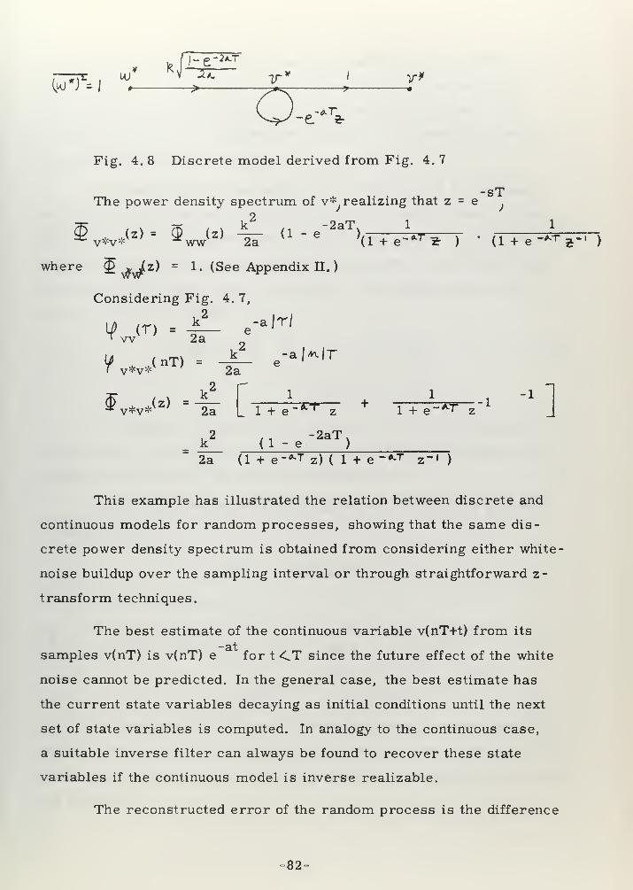
^T-/

Fig. 4. 8 Discrete model derived from Fig. 4. 7

-sTThe power density spectrum of v* realizing that z = e '

2

k(z) = 3L U> 4r (1 - e"

2aT),^v*v*VZ'~ ^wwVZ

' 2aVi_e '(lfe^t ) * (1 + e^r 1

)

where 5 *iz) = 1. (See Appendix II.

)

Considering Fig. 4. 7,

[f (T ) = *L- e-a,T/

' w 2a2

r v*v* 2a

^r , . k2

f 1 1 -1 "1

^ v*v*U) " 2a L 1 + e-^ z+

1 + e"^ z_1

J

2, ,

-2aT,: ( 1 - e )

2a (1 + e-^T z) ( 1 + e-*-T z~' )

This example has illustrated the relation between discrete and

continuous models for random processes, showing that the same dis-

crete power density spectrum is obtained from considering either white-

noise buildup over the sampling interval or through straightforward z-

transform techniques.

The best estimate of the continuous variable v(nT+t) from its

-atsamples v(nT) is v(nT) e for t<CT since the future effect of the white

noise cannot be predicted. In the general case, the best estimate has

the current state variables decaying as initial conditions until the next

set of state variables is computed. In analogy to the continuous case,

a suitable inverse filter can always be found to recover these state

variables if the continuous model is inverse realizable.

The reconstructed error of the random process is the difference

82

between the actual value between sampling instants and the initial con-

dition decay --in other words, the amount of white noise buildup at

the output of the generating model over the sampling interval. This

irreducible error is the fundamental penalty for representing a random

process in terms of its samples.

The result of this discussion is that, from Eq. 4.9, the mean(r

2square error between sampling intervals is

Jdt w (t), where w(t) is

° 1 (T (^ 2

the model impulse response. The average error is thus -=-J 6.T J dt w (t),

It is now proposed that a useful measure of the error due to sampling

is the fractional error power, or the ratio of the mean sqcuare error

to the mean square signal level

T TF.E.P. £. -|" f dr T dt w2

(t) (4.10)

p 2 2dt w (t) = v

This provides a quantitative measure of the inherent penalty for

sampling any random process, regardless of the spectrum shape. An

example will illustrate the utility of this approach.

Suppose the continuous model for an observed random process,

v, is given by

1G(s) =

(s+3) (s+4)

w(t) = e - e

,T -T

e2

. \\*r\ dtw2(t) = jLi| T (i-e- 7T )

1 ,, -6T, 1 ., -8T." 36-T (1 - e

>" 64 T U " e

>

In this form it is difficult to obtain the average square error for

small T, and especially to solve for a T to meet a certain fraction of the

mean square signal level. An alternate route is to expand G(s) in ascend-

ing powers of —

-83-

G(s) =2 J_ J_

IT 5 IT s2

s3

1 + — +s 2

7 2w(t) = t - — t . . .

w2(t) = t

2- 7 t

3. . .

e2

= ^ j]dt w2(t) = X3

" JL T 4

Jjl 12 20

e 3 4FEP = ~ nn = T - 7 T</> (0)

i 2 *° = 14 T3

- 58.8 T4

168

If the FEP is specified to be . 01, an approximate value for T is

given by

T2S(^) 1//3 = .089 Seconds

This section has used the concept of white -noise buildup (1) to

show the mechanism by which sampling of a random process always de-

grades knowledge of the signal, and (2) to present a quantitative measure

of this error from which a rational decision can be made for a proper

sampling interval.

4. 5 New results and interpretations for the optimum filtering problem

A physical system which operates on a given random process

can be viewed as a means of continuously extracting all possible informa-

tion about future values of error from present values of input signals.

An optimum system should result in an error signal e which is on the

average unpredictable from and unrelated to past values of input signal

v. In a linear statistical theory, this lack of relation can only be measured

by a correlation function, which means that

E fv.(t -r) e.(t)) = ^v.e.(r) = ( TJ? O)

\ 1 J il J

(i, j = 1, 2 . . . n)

=84

for a random process with n inputs, under this requirement. Accordingly,

^ o

But e(s)J = i(s)J — W(s ) v(s)_] where W(s) is the optimum

system to be found, and i(sj is the desired output vector. From Eq. 2. 32,

B (s) = cfT .(a) - 2" (s) W^s)* ve -*- vi vv

Therefore,

a'/"1 [gwl.) W

T<s>] **

-1

(g vi( S )]- (2.18)

which is an implicit statement of the optimum multi- dimensional system,

which was obtained with considerable more difficulty (and perhaps more

rigor) in Chapter 2 by an alternate route.

By either method, the basic statement of optimality of realizable

linear systems is then

**' l

{ § ve(8)

}a

°(4.11)

This result will be used to motivate a closer look at the prop-

erties of optimum single -dimensional systems. In particular, the filter-

ing problem will be examined and an optimum unity feedback system

will be derived which takes advantage of some not readily apparent prop-

erties of the standard mathematical solution given by

W (s) =

§\J> A

"I 3T -<s)

77) 1* (2.15)

w Ig*- (s)

Figure 4. 9 shows the basic configuration to be examined. The

following restrictions apply: (1) The signal s is derived from unit density

S/w

V•I Wts)

7® -> e.

Figure 4.9 The basic filtering problem

-85»

white noise passing through a linear system G (s). (2) The noise n iss

derived from unit density white noise, uncorrelated with the signal

white noise, passing through a linear system G (s)5

(3) The signal s

is the desired quantity to be reproduced at the output of W(s) and (4)

W(s) is to be a unity feedback system, with forward transference H(s),

such that W(s) =1+H(s) "

This model is of sufficient generality to include many filte ring

and control problems of practical interest, and its solution will later

motivate a completely general solution.

From Eq. 2.9,

<£ (s) = $ (s) fl - W(s)l - I (s) W(s)ve ss L J nn

= $ (S) ;* - <J5 (S)

H(s)

ssx

' 1 + H(s) nn ' 1 + H(s)

Hence, from the basic equation, Eq. 4.11,

M' x{s^ rrmr}-**'1

{*>rnbr} < 4 - 12 >

Two very important facts are revealed from this equality. Since

the positive poles of Q (s) do not generally equal the positive poles ofS S

Q (s), this equation will only hold in general when (1) the poles of H(s),

which are the zeroes of — „, v , include all the positive poles of Q) (s),1 + H(s)

H(s)and (2) the zeroes of H(s), which are the zeroes of —z 777- v , include

1 + H(s) -

all the positive poles of $ (s). If this were not so, then in the ^.^r-^ nn

partial fraction expansion of both sides, there could not be pole-by-pole

equality. Let -,+v vNn(s)

1

H(s) = -s^T H < s)

f + P _ _where N (s) and S (s) are the LHP poles of $ (s) and y) (s), respec-

P P nn ss

tively, and H (s) is an additional term which does not cancel any of the

signal or noise pole terms.

The optimum system is, from Eq. 2. 15,

=86-

where V (s) equals the LHP zeroes of and solving,1 + rlv S J

N (s) U(s)

H(s) ttt£V+(s) - N+ U(s)z p

+Although this is not obvious by inspection, the polynomial S (s)

* +- ^must be a factor of V (s) - N (s) U(s) in order that Eq. 4. 12 be satisfied,

z paccording to previous arguments.

I v& _ ti^JMSstL

-lj^ss(s)\

This leads to the interesting conclusion that/^"f*+—LaT/ J

which contains only the signal poles, is equal in this case to the sum of

signal poles in a partial fraction expansion of <±> (s), since no cancella-+

wtion of S (s) is allowed. A more general proof of this important identity

will be made later in this section.

Therefore,

H(s) = ^ Signal Poles of ^(s) A jKs)(4 13)

«> Noise Poles of (f\T (s) N(s)

w(s) =H < s > =

S < s >(4 14)mS) 1+H(s) S(s) + N(s)l

' '

This result is of considerable practical and theoretical interest

and applies to all single-dimensional filtering problems, when noise

and signal are uncorrelated. The optimum system determined, W(s),

has the following significance:

The best estimate of an input signal under a mean square error

criterion is that the signal originated from signal poles of a single system,

with transfer function ^ (s) and excited by unit-density white noise.

-87 =

The optimum system then merely determines and sums the canonic state

variables of the signal portion of the random process generating model.

The optimum predictor in this noisy case is intuitively the result of allow-

ing these instantaneous state variables to decay as initial conditions

for the desired fseconds. This is verified by noting that, where the sig-

nal poles of the generating model are^/d J^ss I = "y i , the op-

timum predictor is given by L w * "* r^

ir^ss(s)e

srl ±_ k.e^^^ v £+ J <2J (s) e

s '

1 k. e

wwhich computes and weights state variables for f seconds of initial con-

dition decay.

The above simple interpretation of an optimum system was ob-

tained through rather a roundabout method, and holds only for uncorre-

lated signal and noise and a one-dimensional random process. But having

this result, it becomes simple to extend it to the general multi-dimension-

al filtering and prediction problem with all possible correlations existing

between signals and noise.

The basic equation defining the optimum multi -dimensional system

is the transpose of Eq. 2. 28

W(s) =^ _1<[^

r(s) [g

T(-s) ]

_1

[G_1

(s) (2.28)VI

Also

§ .(s) = G,(s) $T

(s) + G,(s) . $ LS) (2.33)vi d y ss d -x ns

The perfect operation on the signal, G (s), is I for the filtering

problem. Thus,

w(s) --U~l

{$T{

JlCgVs)]" 1

+ $L [gVs)]' 1

} g'^s)

In analogy with the simple case discussed earlier, it is desired

now to prove the^/^ term is merely the result of expanding each elem

of G(s) in partial fractions and retaining only those with signal poles.

88-

First it is necessary to identify the signal poles. Figure 4. 10

shows a multi-dimensional model for the formation of correlated signals

and noise.

G*k<*;

5/G-WAL ^WHITENOISE ^-i-M,

\ SI6N/AL **( i noise.

—

^

Fig. 4. 10 A hypothetical model for the creation of correlatedsignals and noise

Given the auto and cross power density spectra of the signal and

noise vectors, where the noise vector can be of less dimension than the

signal, a (n+m) x (n+m) realizable and inverse realizable matrix filter

G (s) can always be found which can reproduce the observed statistics

of the separate signal and noise components. The poles of the ith signal

are the poles of the ith row of G (s).sn

The matrix of power density spectra of the signal and noise signals

is given by G (-s) G (s) which in partitioned form is

G (-s) G' (s) *sn sn

ss(?)

Lns nn

The positive poles of the ith row of G (s) appear only in the ith

column of the above partitioned matrix. That is, the positive signal poles

appear only in the sub-matrices V (s) and ^

noise poles only appear in $ (s) and § (s)

appear only in the sub-matrices $> (s) and Q (s), and the positive

sn nn

Considering the observed random process v, where v = s + n

and zero elements are permissible in n

w§£) =w

_ss ~ns

G(-s) G"r

(s)

sn nn(2.31)

(2.27)

G (s) = G \-s) S§ (s) + <£ (s)\ + G'Vs)/^ (s) + 1* (s)"\| ss ns j ] sn -1- nn

J

-89-

G(s) =m» T) ss

+ |&T

} [G

"1( -S)

lT

*foa) + E>>}£^>]But G(s) has no RHP poles.

+ "

Since the first and second bracketed terms above have only positive

signal and noise poles, respectively, they are immediately identified as

the separate signal and noise terms in a partial fraction expansion of G(s),

which is the desired proof.

Let GKs) = S(s) + N(s) , where all the signal and noise poles are

grouped together in S(s) and N(s) , respectively. Of course, if one or

more signal poles are identical to a noise pole, the contribution of these

signal poles to S(s) would be obtained through their separate partial frac-

tion expansion in^ < G (-s) (j^ (s) + G (-s) ^ (s) I, since

they could not be separated in a partial fraction expansion of G(s). The

optimum filter is then, from Eq. 2. 28,

W(s) = S(s) [s(s) + N(s)]_1

(4.16)

A unity feedback system is readily seen to have a forward loop

transmission

H(s) = Sts] N(s)~*

(4.17)

and has the appearance of Fig. 4. 11.

Vft i A./" '/c » > S(s;j * M (S J

Fig. 4. 11 A canonic optimal multi-dimensional filter

Fig. 4. 11 is invalid if N (s) is singular, which would be the

case if one or more of the input signals is uncorrupted by noise. In this

case, the canonic configuration of Fig. 4. 12 is still applicable, providing

-90

the trivial restriction of signal having to be present in all input compo-

nents of v is satisfied.

V +&Ncs; Sls)

Fig. 4. 12 An alternate optimal multi- dimensional filter

These optimal configurations have an interesting interpretation

as systems which compute inner signal levels of an effective random pro-

cess generating model, G(s) = S(s) + N(s) . As shown in Figure 4. 13,

the optimal configurations merely act to reproduce quantities which exist

at the input and outputs of the signal and noise portions of the model.

—>» S(*J$*

V +*UJ

:\

i- N~c4;-—

>

S(})s*

!

+

r —^-

—*NO)

-n*

, *

">

\a)

1

> S($j

; s*r — 1 1

—

>

—=J Nts)

A\* Nty «

—

S~(s;

Fig. 4. 13 Signal reproduction in optimum configuration

24Kalman and Bucy recently presented an approach to the optimum

filtering problem which considered the special case of pure white noise

corrupting all input signals, with no cross -correlation between signal

or noise. They postulated a model of the original signal generating model

which appeared in the forward path of a unity feedback system. In the

light of the above analysis, it is easy to see why they were unable to ex-

tend their results, since, from Fig. 4. 11, the model which should have

been specified is the signal generating portion S(s) of the hypothetical

model G(s) -- which creates the actual signal observed and not the pure

=91-

signal component.

The results of this section are particularly important, both in

understanding and in operating on random processes with linear systems.

In essence, it has been shown that the physical system found from factor-

ing a matrix of input power density spectra contains in its signal levels

all the knowable information about the random process which can be ob-

tained by linear measurement of the random process. The optimum system

has the simple form S(s) / s(s ) + N(s)| , where S(s ) contains all the signal

poles (positive poles of (P (s) and Q (s) ) in a partial fraction expansion-

element by element -- of G(s), the effective generating system. Figures

4. 11 and 4. 12 show canonic forms for optimum feedback systems to filter

the multi -dimensional random process.

4. 6 Correlation functions and initial condition responses

Auto and cross -correlation functions have an appearance similar

to the dynamic behavior of linear systems, usually decaying to zero ex-

ponentially as T becomes very large. This section will relate the corre-

lation functions to the initial condition response of the white-noise driv-

en linear model for the random process with an equation of considerable

simplicity and generality.

First, suppose that the cross-correlation function fx.x,(f) isi J

known between two state variables, x. and x., that are defined in a linearJ

system by the general equation

-rr x = Ax + D w (4.1)

where x is the n-dimensional state vector, and w is a r-dimensional

white noise vector.

Since from Eq. 2.9,

3? x.x.(s) = s ^x.x.(s)J J

^x.x.CT) = -jr^x.x.CT) = E{x.(t) . x.(t+T)}

-92-

But /yv. f

* x.x.(T) = £ a.k

E{x.(t) . x^t+T)} + 2 djk

E {x.(t) wk<t+T)}

E {x.(t) . wk<t+T)} =0 (T* > o;

since future values of white noise are not causally related (ie: correlated)

to present values of system signal level (or, more formally, since ir x.w,(s)

contains only RHP poles). Thus,

-^ V x.x.(f) = ± a.. Wx.xAT) (T>0)dr i j ^ =/jk lk

Writing this equation in matrix notation,

if IT) = f <r> aT (t>o)dT* xx ' xx

Transforming,

^" 1

{|^!)

} -^.0) **'*{L£»l -£

But, from Eq. 4. 4

[is-A]" 1- *[e At

]

Transposing,

yT(r) = e

AT¥

T(0) (T->0) (4.18)

XX XX

2This is the desired general relationship, which shows that the n

correlations between state variables in a linear system are mapped

through time by the same transformation that governs the decay of the

A tstate variables in the linear model: x(t) = e x (0) .

Now, it remains to use this result in order to show the meaning

of the correlation functions which would be measured at the outputs or

-93-

output of the random process. Suppose that the r-fold output vector v

is obtained through multiplication of the state vector x by a rxn matrix _R

The cross -correlation function of two output signals is thus

Or in matrix notation

^ (T) = R V (T) R TVV ' XX

For T?0 , using Eq. 4.18

At] T JTW ' XX

If (T) = R (f (0) [eAr

] R

Transposing,

tp^jm - _R e_^ [r_ ^(0)1T

<T>0>

Since Vv.x.(T) = 2 r,, ^x x.(T) or1 J l?s I

lk * J

^ (r) = r </> <r>' VX 'XX

then

(P

T(T) = R e

Ar^T

(0) = R eAr

<f (0) (T^o)(4. 19)' w . 'vx VX

This equation is in proper form to permit interpretation of the

output correlation functions. The initial condition response of the system,

viewed at the output, is

v(t) = R eAt

x (0)

Therefore, if the vector x(0) is set equal in the model to ^xv.(O) =

rv.x(O) then the transient observed at the ith output terminal will be (/V.v.(f),l

ri j

In words, this means that the cross (or auto) correlation function, ^v.v.(T)

between two signals in a random process is the transient which would be

observed at the jth signal location when each of the system state variables,

x, is initially set to (fhtv.(O) and the system released.

-94-

This result tends (1) to re-emphasize the basic nature of the

hypothetical model which is capable of generating a given random pro-

cess, and (2) to interpret the correlation function as a transient of this

model.

4. 7 Advantages of the state and model approach to random processes

This chapter has been written in the hope of altering current ways

of approaching the visualization and study of random processes by the pre-

sentation of a simple explanation for the mathematically-complex results

of contemporary theory. In a sense, the basic question is whether one

should look at what a system does or whether one should look at what a

system is.

It was necessary to first ensure that such a system can always

be found from auto and cross -correlation functions of a multi-dimensional

random process. This was the contribution of Chapter 3. With this assur-

ance, the conventional Wiener theory could be reworked with complete

generality.

Section 4. 3 considered the optimum predictor configuration. It

was shown that this problem is only a matter of continuously measuring

the state variables and weighting them by their initial condition decay

for T seconds.

Section 4. 5 dealt with the problem of filtering extraneous noise

from a desired signal. In this case it was shown that the equivalent gen-

erating model was actually two systems in parallel, one associated with

the signal and the other with noise. The optimum filter merely computed

the output of the signal portion. With the recognition of this simple inter-

pretation, two general canonic feedback arrangements were found which

should be of considerable interest in control systems design.

In section 4.4 a quantitative measure of error due to sampling of

a random process was presented. This was determined from the buildup

-95-

of white noise between sampling instants in the model.

Section 4. 6 showed that correlation functions can be regarded

as transient behavior of the effective model under certain initial con-

ditions .

In all these results, the ideas of white-noise excited system

and system state play the dominant role. "State" and "system" are far

more general terms, however, then their use here would indicate. It is

interesting to conjecture at this point how these concepts might aid the

study of non-stationary and non-linear random processes.

First, in the case of non- stationary random processes it seems

highly probable that the conceptual results derive d in this chapter remain

valid, providing that the effective linear time -varying model for the gen-

eration of the process is known or can be found. The optimum predictor

could still neglect future values of white noise and use only present values

of system state, but of course in this non- stationary case the initial con-

dition decay would no longer be described with the matrix exponential.

Also, the case of finding a time-varying inverse of the effective generat-

ing model in order to recover the state variables appears possible if ex-

tremely difficult. Further promise in this respect is lent by recent work24

by Kalman and Bucy who have derived an optimum time -varying system

which remains similar in form to the stationary case.

In the case of so-called non-linear random processes, which are

distinguished by decidedly non-Gaussian probability distributions, it is

appealing to hypothesize that they occur as the result of independent white

noise driving a suitable non-linear system. Further, from current work25

in this field, for example by Bose , it appears possible that such a non-

linear system might be a finite -state linear system driving a memory-

less non-linear function generator. This is an interesting alternate ap-

proach to the study of non-linear random processes which is more ap-

pealing to the engineer than the more general and highly-mathematical

-96-

26treatment of, for example, Wiener

In short, it is hoped that the simple physical interpretation of the

optimum linear systems presented in this chapter for a stationary random

process will motivate a similar approach to more complex stochastic

problems.

-97-

CHAPTER V.

RANDOM PROCESSES AND AUTOMATIC CONTROL

5. 1 Introduction

Stationary random processes have been examined in the previous

chapters with an eye toward delineating the recoverable information which

exists as a result of optimum linear operations on the signals. The con-

cept of a generating model, excited by white noise and possessing state

variables, has been shown to be a particularly effective way to visualize

the action of optimum systems -- that they perform essentially a measure-

ment or signal recovery of certain quantities in the generating model.

The time has now come, however, to consider how this increased

intuitive understanding of random processes can be of help when control

decisions must be formulated as a result of the information received.

The general control problem is of great interest to mathematicians and

engineers alike, and most significant control problems involve signals,

wanted and unwanted, which are random in nature. In this chapter we

restrict attention to the following situation:

A fixed linear system exists whose output is to be forced to follow

a stationary random input signal, which in the limiting case of a regulator

is constant. Corruption of the command signal with noise is allowable.

Also, load disturbances may be present which are stationary random pro-

cesses uncorrelated with the input signals. Finally, the controller con-

figuration is completely arbitrary as to the possible use of linear and

non- linear elements, with the single important limitation that the con-

troller output signal which drives the fixed system be limited in ampli-

tude to correspond to the saturation level existing in the controlled system.

Section 5. 2 considers the scalar problem and develops a design

philosophy which appears to have considerable promise in the optimum

-98-

control of saturating systems. The particular problem of load disturbance

in linear and saturating systems is treated in Section 5.3. With this foun-

dation, contemporary approaches to full-throw control which can be found

in the literature are critically analyzed in Section 5. 4. Finally, Section

5. 5 presents an extension to the determinate Second Method of Lyapunov

to include random processes. This leads to a design procedure suitable

for a multi -dimensional saturating control system, optimizing a quadratic

error criterion.

In the past chapters general equations, simple proofs, and sweep-

ing statements could be presented with mathematical aplomb because

of the simplicity and power of linear methods of analysis. But in this

chapter the spectre of saturation has arisen to confound our linear theory

and the whole tenor of this thesis must change. No longer can general

quantitative statements be made concerning system behavior; it is diffi-

cult enough to make useful qualitative observations. We must be content

with small nibbles at this frontier of control theory and recognize that

the verification of original ideas can only come with computer analysis

and can only be valid for the specific cases investigated.

5. 2 Saturation and control in a stochastic environment

It is profitable to consider again the optimum unity feedback con-

figuration derived in section 4. 5 for the recovery of one-dimensional

signal from noise, This is shown in Fig. 5. 1 where the input signal v

is composed of two hypothetical components, signal s* and noise n*, which

—> S(4)s*

U) &' > Nw

/h*

-If

*'

W)bJ

SO)

Fig. 5. 1 Optimum filter configuration

-99-

are the best estimates of the actual signal and noise in a mean- square

sense. This minimization of mean-square error means that s* is the

expected value of the actual signal component, conditioned on a physi-

cally-realizable linear recovery. In the system depicted in Fig. 5. 1,

the expected value of error at every instant is equal to zero, since the

output is the expected value of signal. Now, from section 4. 3 it is known

that the expected future value of signal in a linear system excited by white

noise is derived from the decay of the state variables. Applying this fact

to the optimum filter, it is seen that at every instant the expected value

of error is zero for all future time because the output element S(s) has

the same state variables as S(s) in the generating model and they both

are not further excited (as w remains zero in both configurations). There-

fore, an alternate statement of optimality in the linear filtering problem

is that the expected value of all future error be zero at every instant.

With this interpretation, the use of a mean-square error criterion is

seen not to lend much emphasis to the squared-error per se, but rather

it acts as a mechanism for reproducing expected values.

The reason for the emphasis on the particular use of a mean-

square error criterion in the linear theory is that when saturation occurs

in practical output equipment it does not necessarily mean that the op-

timum non-linear control system must be designed on a mean-square

error basis to be consistent with linear random process theory. In other

words, the random process generating models emphasized in this work

contain internal signals which should be the recovery goals of a non-linear

saturation- limited practical control system, but the measure of error in

recovery is entirely at the discretion of the designer.

Since the optimum linear system is constructed so as to make the

expected value of error zero for all future time, a logical choice for a

saturating design criterion should obviously involve this expected future

error, which is, of course, the best information available at any instant

for future use. A convenient way of decomposing this future value of error

= 100 =

is to consider the initial condition decay of random process and fixed

system state variables as one component, designated e(T), and the re-

sponse of an otherwise "empty" fixed system to the future output of the

controller, c(7"), as the other. With this division, the job of the controller

at any instant is to formulate and execute the initial action of a plan that

will make c(f) equal to e(T) as rapidly and efficiently as possible --a

pursuit problem.

It is important that this viewpoint be understood in order to follow

the presentation in this section. The effect of all past input and control

signals is summarized in the state variables, which are in turn used to

represent the expected value of future error without further control, e(T).

In most cases of practical interest the control plan c(T) will start at zero

and must lie somewhere on or within the boundaries formed by the appli-

cation of either maximum positive or negative step inputs to the fixed

system. Fig. 5. 2 shows two possible control trajectories for a given

+ / Response To/j m/\x, m0m positive step

FUTURE- TIM I

Fig. 5. 2. Possible control trajectories

e(T), where c.(T*) is obviously better than cAT) since it reduces the

expected future error more quickly. In formulating this plan, the con-

troller must select for each future instant some value of command signal

within the saturation constraints, preferably to satisfy some design con-

dition of optimality. Then it must execute the initial command of this

sequence, and in the next instant the following changes will occur:

= 101

(1) The state variables that were previously in the fixed system

and the random process generating model will decay as initial conditions,

as indicated by e(T).

(2) The controller command signal will have perturbed the fixed

system state variables, as indicated by c(f).

(3) White noise will enter the random process model and further

change these state variables.

Because of the change in (3) above, the previously computed ap-

proach plan of the controller is no longer valid, and a new one must be

computed. This frustrating need to solve for an optimum c(f), use only

the initial action, and then discard it an instant later is caused by the

fact that we have imperfect knowledge of future events and must "muddle

along" with the currently available information.

The use of expected future error is a very significant formulation

of the problem of control in a random environment, for it transmutes a

stochastic problem into a determinate one that is solely a function of the

state variables of fixed system and random process generating models.

Some possible criteria and general means of solution are presented

next, followed by a more detailed look at a particular design which has

the virtues of near optimal performance and easy mechanization.

The most general approach to this problem would employ the

techniques of dynamic programming, which in this case would attempt

to minimize some integral of a function of the state variables over all

future time as the error approached the zero or equilibrium condition.

To accomplish a valid solution by this means, thereby developing a con-

trol decision as a function of all the state variables, would require con-

siderable ingenuity, very large amounts of digital computation, and is

properly outside the scope of this report. The mechanization of the solu-

tion would in general involve a table lookup capability for the control system.

102-

Another valid criterion for the design would be one of time-op-

timality. In analogy to the determinate or bang-bang regulator problem,

which specifies that the time required to make all the state variables

of the controlled system equal to zero should be minimized, one could

demand that the future expected error and its defined derivatives be

brought to zero in the quickest possible time. It has been proven in most

determinate cases that full-throw or maximum effort control yields a

minimum time solution.

Thus a set of transcendental equations could be easily written to

equate the expected value of error and its n-1 derivatives to zero at some

future time after n switching intervals, where n is the number of state

variables in the controlled system. If these equations could be continuously

solved to determine the duration of the first switching interval, then the

switching time of the control system would occur when this switching

interval became zero.

Unfortunately, the actual real-time solution of these transcendental

equations appears quite difficult, assuming that a solution even exists.

One source of difficulty is that the dependent variables, the switching

times, must be constrained to be positive and in a certain order corres-

ponding to successive sign changes of the control variable.

Another more abstract objection can be made to the criterion it-

self. First of all, the fact that the expected value of error and its defined

derivatives are zero at a certain future time does not ensure that they will

remain zero over the remainder of the interval, unlike the determinate

case, since the saturation of the controlled system may prevent it from

following exactly the further decay of the random process state variables.

Next, the existence of a future value of zero of this expected erTor and

associated derivatives does not necessarily mean that the intermediate

values of error in transit were small. That is, the requirement that the

error derivatives be brought to zero simultaneously may cause the con-

-103-

troller to select a trajectory which is obviously less desirable than one

which approximately "matches up" at a considerably earlier time.

In the two approaches considered, the dynamic programming and

the time-optimal, it is clear that there are very difficult analytical pro-

blems as yet unanswered, and that the sophistication (and consequently

cost and size) of the control equipment must be relatively high. Is there

then no way of practically utilizing the state variable approach to random

processes in control? In the remainder of this section we shall discuss

a proposed scheme of single-dimensional design which has many appeal-

ing features, not the least of which is the ease of instrumentation. Then,

in Section 5.5 a comparatively simple multi -dimensional saturating con-

troller will be described which is based on an extension of the Second

Method of Lyapunov. The case of load disturbance will be dealt with in

Section 5.3.

First of all, it is useful to reconsider the objectives of using the

expected value of error in a design criterion. By constructing a non-linear

system which would reduce the expected value of future error rapidly if

white noise were suddenly cut off, it is hoped that the truly optimum

linear system will be closely approximated. This hope is based on the

observation that the optimum linear system produces, if white noise

were cut off, a zero value of error for all future time. An alternate

interpretation is that the best estimate of future error is its expected

value. A decision scheme for control that always tends to reduce this

expected future error in an efficient manner will, on the average, yield

desired performance under the constraint of saturation and will best

utilize the information about the random aspects of the problem available

from linear theory.

Full throw or maximum effort control is selected in order to

capitalize on, rather than linearize, the saturation in the output equip-

ment. This will guarantee that the mean-square corrective effort is at

an absolute maximum. Also, it has been proven an optimum mode in time-

-104-

optimal determinate control systems.

The simplest criterion to use would be that the future error become

zero in the smallest time. This would be nothing more, if full-throw

control were used and there were no noise at the input, than an error-con-

trolled relay. This is patently not a very satisfactory solution, for the

large error derivative which would usually result at the instant of zero

error would ensure a large error before the next zero crossing -- possibly

an unstable buildup would occur.

However, if it were specified that the future error and the error

rate should be brought to zero simultaneously in the quickest possible

time, then the result of non-coincident second and higher order derivatives

between desired and actual output would have a definitely much smalte r

effect on the amount of later error. This specification would mean that

the error would be brought to controllable proportions in the shortest

time.

It is much easier to understand these ideas with the aid of typical

control trajectories. Figure 5. 3 shows a curve of expected error with no

Fig. 5. 3 An almost time-optimal control trajectory

further control, e(T), and a superimposed planned control trajectory,

cCT). The controlled system of this example is assumed to include an in-

tegrator, and the initial path of c(T) corresponds to the step response

of this system to a positive saturation-constrained input command. At

-105-

time Tl the sign of the control variables is changed from + to -, and the

expected future error, which is the difference between e(T) and c(T~),

is brought to zero with zero rate at timet"- .

Figure 5. 4 shows a similar error plot, only the problem has ad-

vanced to timeT. . The new e(T") is the expected value of error with the

new c(T) set equal to zero for all time greater than Tt, which corresponds

to the difference between the e(T) curve of Fig. 5. 3 and the dashed path

indicated by "0 at T*"

T"

Fig. 5. 4 Switching time determined by tangency

The very significant fact demonstrated in Fig. 5. 4 is that the time

to switch from + to - is 'K because at that time e(V) first becomes tangent

to a cCfi representing the negative applied step. On the basis of this, we

can postulate a control law for the proper sign of the current full-throw

forcing variable, which is the desired output of the controller. If c+Cf)

and c-(T) are defined as the step responses of the controlled system under

maximum positive and negative steps, respectively, then the current

forcing function should be either + or - depending on whether the most

future intersection of e(f) is with c+(T*) or c-(T). This switching law al-

ways yields an output which continually seeks to reduce large errors with

maximum effort, and switches at the last moment (when the tangency first

106-

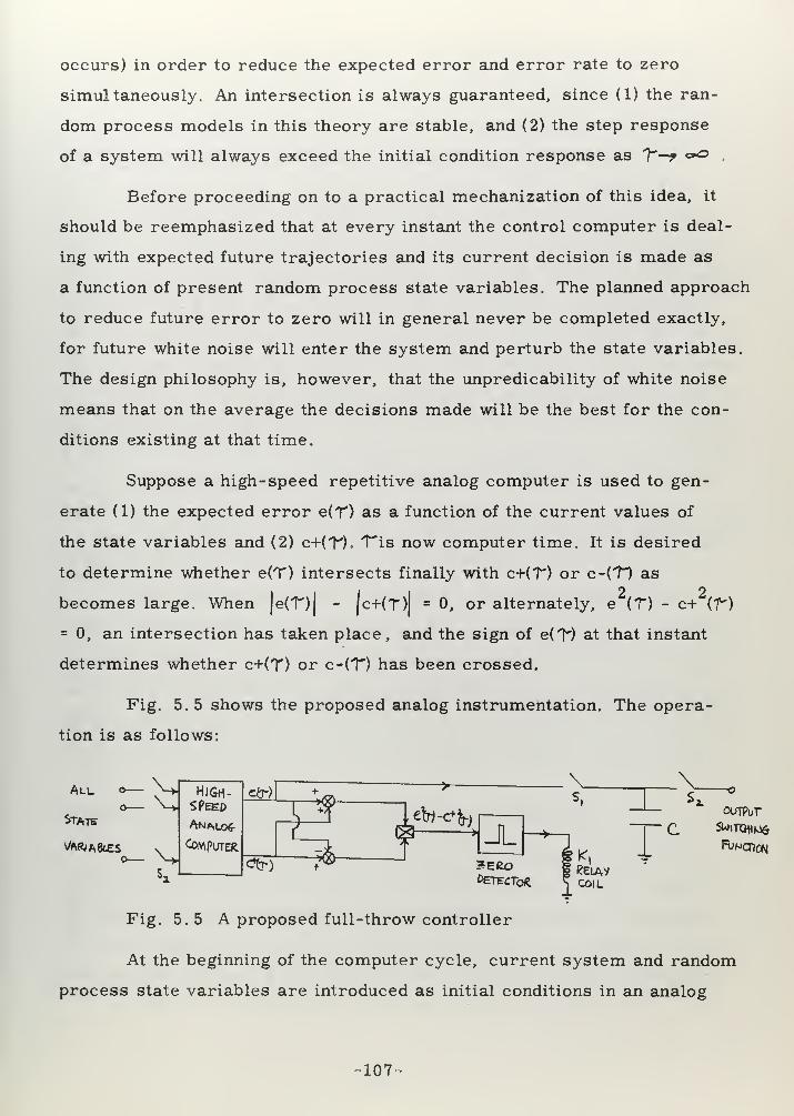
occurs) in order to reduce the expected error and error rate to zero

simultaneously. An intersection is always guaranteed, since (1) the ran-

dom process models in this theory are stable, and (2) the step response

of a system will always exceed the initial condition response as 7*—9 <s»°.

Before proceeding on to a practical mechanization of this idea, it

should be reemphasized that at every instant the control computer is deal-

ing with expected future trajectories and its current decision is made as

a function of present random process state variables. The planned approach

to reduce future error to zero will in general never be completed exactly,

for future white noise will enter the system and perturb the state variables.

The design philosophy is, however, that the unpredicability of white noise

means that on the average the decisions made will be the best for the con-

ditions existing at that time.

Suppose a high-speed repetitive analog computer is used to gen-

erate (1) the expected error e(T) as a function of the current values of

the state variables and (2) c+(7"). fis now computer time. It is desired

to determine whether e(T) intersects finally with c+(T") or c-(T) as

becomes large. When |e(T)| - |c+(T) = 0, or alternately, e (T) - c+ (f

)

= 0, an intersection has taken place, and the sign of e(T) at that instant

determines whether c+(T) or c-(T) has been crossed.

Fig. 5. 5 shows the proposed analog instrumentation. The opera-

tion is as follows:

All o

Statsoutput

S^iTOtiUfc

Function

Fig. 5.5 A proposed full-throw controller

At the beginning of the computer cycle, current system and random

process state variables are introduced as initial conditions in an analog

107

system which will reproduce e(T) and c (T) at its output when released.

With the trivial identity, e2(f) - c

+2(T) = ]jt(T) + c* (T\\ [e(T-) - c^(rj),

the intersections of e(T) and c (7") result in an output from a zero-detect-

ing device (perhaps a suitably configured relay with a small dead zone)

which energizes coil K^, momentarily closing switch S... Capacitor C

then "remembers" the voltage e(T') according to the previous zero cross-

ing. After a suitable run, the computer is recycled, and the programmed

closing of switch S delivers the last e(T) voltage at the output. This sampled

signal has the sign of the desired polarity of the maximum command to

the fixed system; further, it becomes zero when the present and future

error becomes zero. This makes it a desirable switching function to drive

a command relay with an arbitrarily small dead zone which will prevent,

for example, a continuous cycling under zero error conditions. Alternately,

a limiter with very high but finite gain near zero input can be used as the

output command element.

The computer repetition rate is chosen so that an error of one cycle

in switching will have small effect on the accuracy of control.

This configuration has the virtues of (1) being applicable to any

scalar linear system which saturates and any random process, regardless

of order, (2) being based on a design criteria which is intuitively satisfy-

ing, and (3) being the first practical design offered for a saturating control

system which uses all the available statistical information and tends to ex-

ploit rather than linearize away the incontestable saturation phenomenon.

5. 3 Optimum feedback configurations with load disturbance

The previous chapters have been mainly concerned with extract-

ing useful information from an input signal. In a control system, one of

the reasons for using feedback is that a disturbing signal often exists at

the output equipment. Figure 5. 6 shows the conventional means of mani-

pulating a disturbance d inside a loop into a form which can be dealt with

-108

or + 4- v^Sh W ^sb-

Fig. 5. 6 Manipulation of load disturbance to obtain standardcascade configuration

in the standard theory. This is the approach taken by Newton, Gould and

Kaiser and by Smith . There are two difficulties with this step however.

The first is that the form of the feedback path must be assumed. Secondly,

and much more important, the preliminary dilution of disturbance and in-

put signal creates an unnecessary task for the optimum system in separat-

ing them again.

It will be demonstrated in this section that in a linear theory load

disturbance does not affect the basic statistical design. As a start, one

optimum system which theoretically reduces the effect of load disturbance

to zero and yet operates optimally on the input signal is given in FigureS(s)

5. 7. Here —.—

r

_ T/ ; is the optimum system proven in section 4. 5,S(s) + N(s) r j r

where 5 (s) = G(s) G(-s) and G(s) = S(s) + N(s), the signal and noisewcomponents, respectively.

K- <=o

or Sc?)

SC?)-»-N(s) 2* K £&

Fig. 5. 7 Elimination of load disturbance with infinite gain amplifier

A more practical elaboration of this scheme is given in Figure 5. 8,

which shows an arbitrary transfer function H(s) enclosed with a minor

loop with infinite gain. This configuration is of considerable practical

significance since it is optimum, compensates any fixed minimum-phase

transfer function, unless the excess of poles over zeroes of H(s) is such

-109

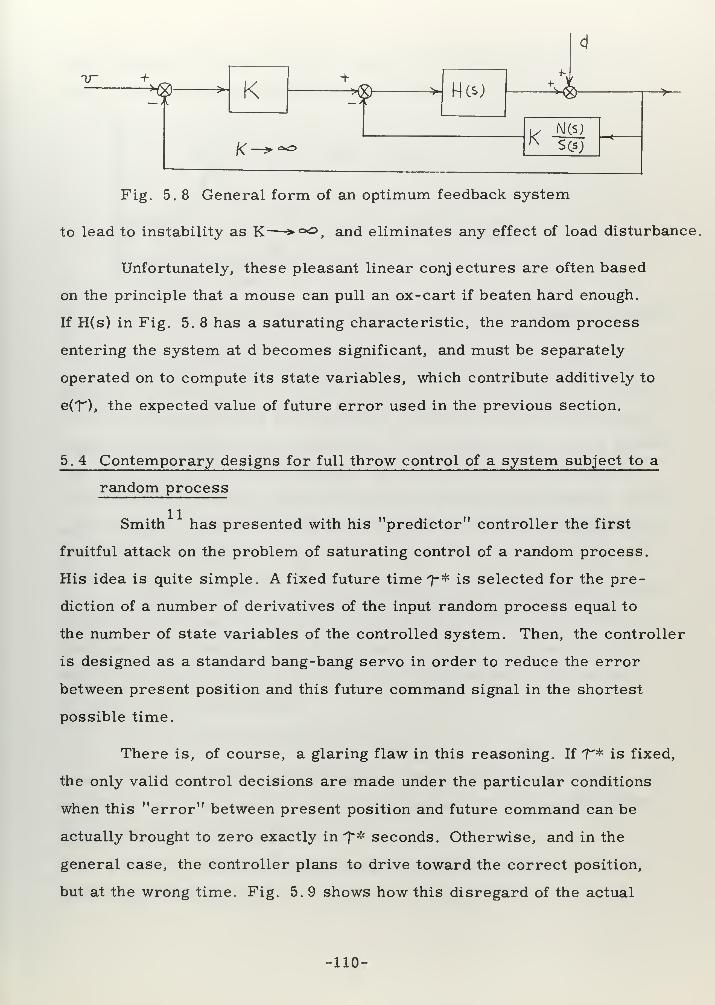
d

ir +K

+^- Hcs; ^Mgh

fcoO K

ncs;

Fig. 5. 8 General form of an optimum feedback system

to lead to instability as K—J* *, and eliminates any effect of load disturbance,

Unfortunately, these pleasant linear conj ectures are often based

on the principle that a mouse can pull an ox-cart if beaten hard enough.

If H(s) in Fig. 5. 8 has a saturating characteristic, the random process

entering the system at d becomes significant, and must be separately

operated on to compute its state variables, which contribute additively to

e(T), the expected value of future error used in the previous section.

5. 4 Contemporary designs for full throw control of a system subject to a

random process

Smith has presented with his "predictor" controller the first

fruitful attack on the problem of saturating control of a random process.

His idea is quite simple. A fixed future time 7-* is selected for the pre-

diction of a number of derivatives of the input random process equal to

the number of state variables of the controlled system. Then, the controller

is designed as a standard bang-bang servo in order to reduce the error

between present position and this future command signal in the shortest

possible time.

There is, of course, a glaring flaw in this reasoning. If T* is fixed,

the only valid control decisions are made under the particular conditions

when this "error" between present position and future command can be

actually brought to zero exactly in 1~* seconds. Otherwise, and in the

general case, the controller plans to drive toward the correct position,

but at the wrong time. Fig. 5. 9 shows how this disregard of the actual

110 =

time required to obtain a change in state can result in poor control deci-

sions, using the display presented in section 5. 2.

IS

•xlu

*&)opt/mum Control tpateot»(2/

Smith v^" vmeController. n State

Fig. 5. 9 Consequences of a fixed T* in the Smith predictor servo

30Benedict based his dissertation on this lack of optimality in an

attempt to justify or discredit this approach with analog computer simula-

tion. His results indicate that this Smith predictor servo is better than a

bang-bang controller which ignores any future change in the control signal

(ie: T* = 0), which is to be expected. He also notes that increasing the

value of T when the input signal level is high improves performance, which

again is logical since the actual time required to reach the specified state

would tend to be larger.

31Hopkin and Wang have taken perhaps a more logical look at this

problem. They make a Taylor's series expansion of the input random

process signal, and attempt to find a set of control switching intervals

which will reduce all the derivatives of the extrapolated future system

error to zero simultaneously.

The two defects in this approach are:

(1) The intrinsic quantities of the random process, the state

variables, are neglected in the Taylor series approximation, this provid-

ing a poor error prediction.

(2) The resulting transcendental equations are difficult to solve,

if a solution exists at all.

= 111

In summary, it is felt that the two attempts discussed above have

merit as beginning steps, but that the problem outline and approximate

solution of Section 5. 2 more clearly define the optimum system and best

utilize the information contained in the input random process.

5. 5 Multi-dimensional bang-bang control of systems subject to random

process inputs

There are three general classes of power actuator in a control

system. First, the output transducer may be conservatively rated and

perform in essentially a linear manner, which allows use of the large badly

of design information on linear control systems. Secondly, it may operate

in a partially saturated condition, the improvement of which case having

been considered earlier in this chapter. Finally, the power actuator may

be fairly inadequate and under- rated for the job presented by the input

random process.

It is this latter case which will be considered in this section. The

corrective action of the controller will not have a pronounced effect on

the error, but it is desired to optimize the effect small as it may be. Es-

sentially, what will be done is to define a figure of "badness" for the state

of the controlled system and of the random process which is a measure

of the expected future error. Then, the control or controls will be con-

tinuously thrown in such a direction so as to maximize the rate of de-

crease of this figure of "badness" at every instant.

The control system chosen for illustration of these ideas is a re-

gulator, but the ideas are equally applicable to a servo application.

To structure this design procedure in an orderly fashion, it is first

necessary to present some results of the venerable "Second Method of

32Lyapunov" . Then, an original modification will be made in order to ex-

tend this determinate theory to include random processes. Finally, it will

be shown how an optimal control law can be found as a linear function of

-112-

the state variables.

The Second Method of Lyapunov is not so much a method as it is

a way of characterizing the free dynamic behavior of linear and non-linear

systems. It uses a type of generalized energy expression, and examines

the rate of change of this function for various states of the system. If this

energy expression, called a Lyapunov function, tends to decrease every-

where except at the equilibrium point in a region of possible system states,

then the system is considered stable in this region.

In the particular case of a free linear system with no external

excitation, the standard differential equation form is

-~ x = Ax (4.1)dt

TA Lyapunov function, V(x), is chosen as a quadratic form x Px,

where P must be positive definite and symmetric. From the results of

section 3.3, it is known that, if P is positive definite, it can be factored

into two matricesTP = N . N

with N having real elements only. Thus,

T Tx Px = (Nx) Nx

which is the square of some linear transformation N on x.

One choice for P might be such as to make V(x) equal the energy32

of the system. According to the Second Method , the system is stable

if and only if — V(x) <C for all x, where x /

d , T , xd T t, f d T~l ^ T^/d 1—j- V(x) = — x Px = <—r; x f Px + x P<tt- *>

but

dt dt 1 dt ) dt

— x = A xdt

^- V(x) = xTATPx + x

TPAx = xT ATP + FA~]

Thus, ATP + PA = -Q (5.2)

-113-

J

where Q is some positive semi -definite symmetric matrix, if — V(x)

is always to be negative for any value of x.

The above relations are very important to the linear theory. Since

v(x,»J dv« x , =f dt ^*> -U (- *%L)

and ,o©

xTPx =

Jdt (x

TQx) (5.3)

the two symmetric matrices, P and Q, provide quadratic forms which areT

related in an integral fashion. Accordingly, if x Qx represents someT

measure of instantaneous error of a free system, x Px is the integral

of this error over all future time, which is a very useful error criterion.

n/n-4- 1 \

Eq. 5.2, in this case, must be solved for P with = inde-

pendent linear equations for a given Q.

33Bass suggested, in the case of a linear system settling to equi-

librium, that one form of good full-throw control would attempt to maximize

the negative rate of change of V(x) at every instant, V(x) being a suitably-

defined error criterion for the system without further control. In this

case

-37 x = A x + D cdt

c being a control vector having an amplitude constraint on each component.

£ [xTPx] . [5_ XT|

px + xTp|d_

xj

Substituting from the matrix differential equation

%- [xTPx] = [Ax + Do ]

TPX + xTp

[ **+ Dcl

T T T "1 T T Tx [_A P + PAj x + c D Px + x PDc

T r -T_ _ A n . T Tf T 1 T T[AP + PAj x + 2 c D Px

since a scalar can be transposed at will and P is symmetric. ThereforeT

to select c. so as to maximize the negative rate of change of x Px

114-

sign c. = - sign | D Px|. (5.4)

and the magnitude of c. should be the maximum possible. P, being a

measure of future error of the system, will be found by postulating a

positive definite matrix Q, which represents the instantaneous error, and

solving Eq. 5.2.

With this admittedly brief account of some of the available techniques

from the determinate Second Method of Lyapunov, it is now desired to con-

sider how this theory might be adapted to include stationary random pro-

cesses, since the state concept has been extended in this work to stochastic

inputs

.

To fix ideas, the regulator problem will be considered. Without

any control action, a physical system H(s) is shown in Fig. 5. 10 being

acted upon by a random process which is hypothesized to originate in a

white-noise driven system G(s). The output e is an undesired error. From

the results of this and the previous chapter, it is known that the expected

value of e(t +T) for Is

"} o is completely specified by knowledge of the state

variables of G(s) and H(s). Therefore it is logical to define a LyapunovT

function, x Px, which represents an integral error criterion over all future

time of the expected value of error from the total state vector. That is,

the concept of system in the Lyapunov theory is enlarged to include the ef-

fective system which generates the random process.

The error e and its m - 1 derivatives are linear combinations of

2 2 • «2the m state quantities of H(s). Thus, e , e , e , . . . can all be weighted

with a non-negative measure of instantaneous undesirability.

di-l

If e = B x, , where e. = —:—=— e, B is a mxm matrix, and x, is

idt

i-l h

the state vector of H(s), and the measure of undesirability of e is given byT T T

e Ee = x B EBx , then the matrix Q to weight the instantaneous undesira-

bility of the entire state vector x is given by

115

U)

Gi?)lr

HO) —>-

Fig. 5. 10 System subject to random disturbance

The first m elements of x are identical to x, .

r°T ^ tThe integral error criterion I x Qxdt = x Px

is found from solution of

AT P + P A - - Q (5.2)

if A is the matrix of the differential equation which governs the entire

systemd

-77 X = A Xdt

Now, suppose that it is desired to regulate the error with con-

trols that saturate and have small effect on the physical system in com-

parison with the random process. Bass's approach, described previosuly

in the determinate case, appears to have considerable promise in this

problem.

The objective of the control system in this case is to maximize

continuously the neg ative rate of change of the measure of future error.

Eq. 5.4 is still valid

sign c. = - sign j D P x I ,

with D defined by

d * ^—- x= Ax + Dcdt

A simple example will illustrate the ease of application of these

ideas:

EXAMPLE

A spring-mass -dashpot configuration is shown in Figure 5. 11. F2

is the disturbing random process, with power density spectrum R(s+a) (-s+a)

-116-

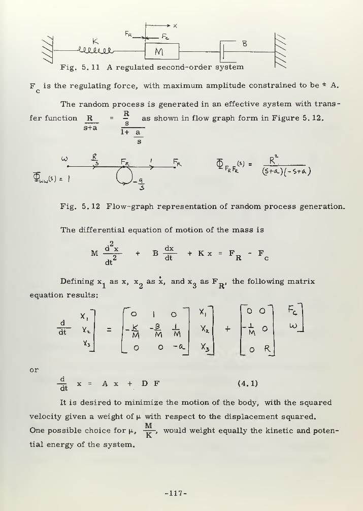
K

* X

MB

Fig. 5. 11 A regulated second-order system

F is the regulating force, with maximum amplitude constrained to be ± A.

The random process is generated in an effective system with trans

-

Rfer function R = — as shown in flow graph form in Figure 5. 12.

s+a =-1+ _a_

s

w->--

3L&) ^ i

s

K'«**. (S-tJL)[-<>-t-&.)

Fig. 5. 12 Flow-graph representation of random process generation.

The differential equation of motion of the mass is

dxM d2x

+ Bdt'

dt+ Kx = F = F

R c

Defining x. as x, x as x, and x_ as F , the following matrix12 o xv

equation results •

*i" fo 1 o X. ~o ol «=t

d

dT v.M

-8M

1

M x* + -*° LO

Vj -0. *3 o R

n

or

— x=Ax + DFdt

(4.1)

It is desired to minimize the motion of the body, with the squared

velocity given a weight of |x with respect to the displacement squared.M

One possible choice for \i, -==-« would weight equally the kinetic and poten-Ktial energy of the system.

= 117-

Q =

Next Eq. 5. 2 must be solved.

AT P + PA= = Q (5.2)

In this example, this equation is readily solved for the 6 independent

elements of the symmetrical P. Solving,

11

33

K2 B

1

MkB m,m( r +A) +

2"K 'P22 " "B ( tk +

2 a M

P =M

.

12 2 K '

B M + a M -t->"-AK MK2 B + a

2 K B M + K B2

P13

= (Ba + a2 M)P

33 =4(| +A)

->U-)

P = a M P^23 33

From Eq. 5.4

Fc

= - A sgn |dT P x } t

f 1 It.= - A Sgn <- — P. _ X. - ~ P,

® l. M 12 1 M : }22X2

=

M P23

X3

_ . Jl 1 ,M^ ijX 1 B + a(yW.K + M)Fc=Asgn

\-2kXl+

2B ( K +A)x2f2K Kfa(aMfB) X

3

Here sgn is an operator which equals + 1 if the enclosed quantity

is positive, and - 1 if it is negative.

This is the linear switching law which continuously tends to maxi-

mize the rate of decrease of the error criterion

jr{E [x(r)]}2

(E [x(r)]}2] dT

iwhich is a function of the state variables.

If it is desired to discount future values of error with an exponen-

tial, e , the matrix A is replaced by A - bl, since the Laplace trans -

}

-118

form of the system is given by j_sl " AJ , which, when s is replaced by

s + (r, becomes j~s I + (rl - Aj

This discounting becomes particularly significant in the case of

a servo, where integrators often appear in the controlled system, because

the integral of the squared initial condition response of an integrator is

infinite, and the design impossible. Replacement of — by ——-. means

a finite square response exists and this procedure is applicable.

To summarize the advantages of this proposed full-throw control

of a random process:

(1) The system becomes more and more optimum as the inadequacy

or non-linearity of the control transducer is emphasized.

(2) The design procedure is simple to execute and results in a

completely linear system except for the output relay.

(3) The resulting system is guaranteed to be stable from the non-

linear part of the Second Method, since y(x) is always negative.

(4) Multi -dimensional designs can be made with no more theoretical,

computational, or hardware difficulty than the single -dimensional case.

These four advantages make this proposed design philosophy very

promising for practical applications where power transducers are inade-

quate for their job in a stochastic environment.

-119-

CHAPTER VI.

SUMMARY AND CONCLUSIONS

6. 1 Outline and summary

The results obtained in this thesis investigation intertwine through-

out the entire theory of stationary random processes. However, there

are three fundamental and significant contributions in this work:

(1) Development of a complete multi -variable theory

The random process with many separate but statistically related

signals -- the so-called multi -dimensional random process -- has been

studied to an extent that there is now no conceptual difference between

single- and multi -dimensional theory. An important analytical tool in

this respect is the equation

§5 (s) = ^ £ G„(-s) ^x.y.(s) H T(s) (2.32)

xy j. j __i i J _Jwhich compactly determines the statistical relations between signal vectors

in a linear system as a function of the properties of the inputs.

The key to the solution of the optimum multi -dimensional system

in the Wiener sense is the concept of matrix factorization, which separates

a matrix of cross -power density spectra among the members of an input

random process v, according to the equation

$> (s) = G(-s) GT (s) (2.27)w .

such that both G(s ) and G(s) represent transfer function of stable systems.

With this factorization, it is possible to represent the optimum

multi -dimensional system with

WT (s) = [gT

(s)]=1

jJ:"1{g

=

\-s) (j5vi(s^<2.28)

The matrix factorization problem is one of great complexity. The

general solution presented in Chapter 3 was reached only after many

-120-

other approaches aborted. It basically consists of a series of simple steps

which manipulate the given matrix into desired forms, of which the final

one is a numerical matrix which can be easily factored. An iterative

method is also presented which shows promise of efficient and rapid so-

lution when a digital computer is used to solve resulting sets of linear

equations.

(2) Introduction of a theory of random processes based on physical models

The results of this thesis indicate that the simplest understanding

of random processes and of the optimum systems which operate on them

is obtained by hypothesizing that some linear system is being excited by

white noise to produce the random process, v. To support this claim:

(1) The result of matrix factorization, G(s) , is such a system,

where G(-s) GT(s) = <J> (s).

(2) The optimum predictor merely reproduces the individual state

variables of G(s) , and weights each by its reduction after "Tseconds of initial

condition decay in the model.

(3) If G(s) is separated into two parallel systems, S(s ) + N(s) ,

associated with the signal and noise components, respectively, of a random

process, then the optimum filter merely recovers the output of S(s) . This

optimum filter is, in canonic form, a unity feedback system with a forward_ i

loop transmission of S(s ) N(s) .

(4) Auto- and cross -correlation functions can be interpreted as

the initial condition response of G(s).

Incidental to this approach, it was found that the fundamental state-

ment of an optimum physically-realizable system is that any resulting error

should be uncorrelated with the past values of any input signal.

(3) The state of a random process viewed as fundamental information for

control use

The state approach has proven a powerful tool in the analysis of

-121-

determinate system behavior. A major contribution of this thesis is the

extension of these techniques to include the study of stationary random

processes.

The output of an optimum predictor minimizes the mean-square

error of the estimate, or alternately, is the expected value of the future

signal. It has been shown that this expected value is merely the initial

condition decay of the current state variables of the effective generating

model.

As was discussed in Chapter 5, the optimum filter at any time t

has a configuration which causes the expected value of future error, e(t+1^),

to be zero for all positive values of T*. Thus, for the purposes of control,

the actual system will more closely approximate the optimum system as

the expected value of future error is minimized.

A typical control problem has an input random process which is

to be followed and perhaps filtered, a fixed linear system which is externally

controlled, and a disturbance which acts on the fixed system. The expected

value of future error is given by (1) initial condition decay of state variables

of the input and disturbance generating models and of the fixed system,

and (2) the effect of future control action on an otherwise "empty" fixed

system. This problem of control becomes quite difficult when an ampli-

tude constraint is placed on the control variable.

Thus, the controller of a saturating system must continuously

select a control variable which is a function of all the state variables so

as to tend to minimize, with some criterion, the expected value of future

error.

Two general and feasible solutions to this problem have been given

in Chapter 5. Both assume that the best operation of the system will re-

suit with full-throw control. The first solution selects for a criterion

that the control variable should switch at an instant when the expected

value of error and its derivative can be brought to zero simultaneously

-122

along the next control trajectory.

The second solution considers the effect of future control as

small, and always tends to minimize a quadratic measure of future error.

This is accomplished through extension of the classical Second Method of

Lyapunov to include stationary random processes. A particularly signi-

ficant result of this approach is that it permits a rational and easily in-

strumented design procedure for a multi -dimensional saturating system.

6. 2 Paths for future research

In the course of this thesis investigation, many problems were

encountered which could not be satisfactorily dealt with in this report.

The following discussion presents some of the more prominent of these

in the hope that further interest and research can be stimulated.

(1) In many random processes of practical interest, for example,

the national economy, there are available a great number of possible com-

ponents for a multi -dimensional analysis. Assuming that this stationary

theory might approximate the true behavior (which would probably not be

valid) it is interesting to conjecture what might happen as the number

of scalar processes used becomes very large. Since the error in predic-

tion of a variable, for example, is always made less as the dimension

of the random process increases, one intuitively feels that the prediction

error could be made arbitrarily small by analyzing enough processes

which cross -correlate with the variables of interest.

It would be interesting to obtain some measure or bound on the

increase in precision obtainable by considering an additional correlated

random process, without completing a refactorization. Also, a means

of selecting the most useful (in the sense of reducing prediction error)

members of a set from consideration of their correlation functions is

needed.

(2) A general solution was presented in Chapter 3 for the matrix

-123-

factorization problem. The resulting answer for G(s) can be multiplied

Tby any real unitary matrix U, where U . U - I, without affecting the

validity of the answer. Although existence has been proven, uniqueness

has not. A useful further addition to this theory would be a proof of this

uniqueness of G(s) -- or, by counter-example, that a multiplicity of answers

exist besides the unitary transformation.

(3) Two significant alternate statements of optimality for linear

systems have been found through analysis of the Wiener theory.

(a) Zero correlation exists between present error and all past values

of input signal.

(b) The expected value of all future error is zero at any instant.

Considering (a), this could be generalized to the non= stationary

and "non-linear" case by specifying that all measures to indicate statistical

relation between signals be zero between past input and present error.

In the case of (b), this statement appears to be just as basic as re-

quiring that the mean-square error be minimized. This appears to have

an immediate application to random processes which are non=stationary

and/ or non=Gaussian.

The viewpoint of the author is at variance with much of the present

work going on in non-linear random process theory. It is suggested that

a possibly fruitful (although modest) line of attack would be to specify simple

non-linear models for the creation of the process from independent white

noise, and determine suitable statistical measurements which could fix

the parameters of these models. This approach is in contrast with a theory

which attempts to be totally general (ie: Wiener ) but which results in

models which have an infinite number of state variables. If a finite- state

model -- perhaps a linear system followed by a memeory-less non-linear

function generator -- could be found to represent adequately a class of

random processes -- then the optimum configurations for systems to operate

on these processes could be found through extension of the state and model

-124-

concepts outlined in this work.

(4) Practical control of systems operating in a stochastic environ-

ment will generally involve considerations of saturation, unless the de-

signer is willing to pay for the validity of the linear theory with increased

power actuator size, weight, and cost. The optimum controller has been

shown, in this case, to be one which continually plans to reduce the ex-

pected value of future error to zero in some optimal fashion.

There appears to be considerable promise in attempting a dynamic

programming solution to this most important problem. If a maximum

effort control system is specified, the desired solution is the delineation

of the switching surface as a numerical function of the state variables

of the random process and of the controlled system. A useful approxima-

tion to this surface would be its Taylor series expansion as linear and

quadratic functions of the state variables.

The two proposed designs of Chapter 5 have the advantages of (1)

comparatively uncomplicated instrumentation and (2) rational design theories

which make use of the state concept and the known saturation limitations

of the control signal. A complete analog computer investigation of their

merit would be warranted for comparison with more conventional configura-

tions.

-125

APPENDICES

-126-

APPENDIX I.

OPTIMALITY IN DISCRETE LINEAR SYSTEMS

1. Introduction

The random signals which have been the concern of the main part

of this report have been continuous in time, as have been the systems which

act on them. However, many problems of physical interest deal with random

sequences of numbers -- perhaps equally-spaced samples of a continuous

random process - and associated linear discrete systems.

There are several good textbooks -- for example, Ragazzini and23

Franklin -- which adequately present sampled-data theory, both deter -

minate and stochastic. In all, the primary emphasis has been on auto-

matic control applications, heightened by the increasing use of digital

computers in control.

The purpose of this appendix is not to encapsulate this general

discrete theory, but merely to show how the major results of this partic-

ular work in continuous random processes are easily extended to the

case of stationary, ergodic, and discrete stochastic processes. Pertinent

equations are preceded by the number of their analogous continuous equa-

tion in brackets.

2. Fundamental properties of discrete signals and systems

A discrete signal is a sequence of numbers, such as

.... f(n - 1), f(n), f(n + 1) ....

with n indicating discrete time. A "z -transform" is defined by

„, „ v n-1 ., v n .. , v n+1. . . + f(n - 1) z + f(n) z + f(n + 1) z ...

where the transform variable z serves to index the associated f(k) to the

proper time. For example, the sequence2 3 k

x , a, a,a,....,a,..»

-127-

has a z -transform2 2 k k

1 + az + a z +.....+ a z1 - a z

The variable z acts as a unit delay operator. Discrete systems

are constructed with this building block to delay, sum or multiply by

constants the discrete variables which pass through it. A convenient way

to visualize this process is to consider the discrete signal as a series of

impulses with areas equal to the value of the variables. The discrete

=sTsystem is then denoted by a transfer function in z, where z = e . T is

the time interval between impulses. This representation allows immediate

extension of much of the continuous Laplace transform theory. In example,

if x(n) is the input sequence, y(n) the output sequence, and the system

transform is given by G(z), then

Y<z) = X(z) . G(z)

3. Statistical relationships

The cross correlation function between two discrete signals, x(n)

and y(n), is defined by [2. 3 ~\

^x (k) = E ^x(n) y(n + k)} (A 1. 1)

and the discrete "cross power density spectrum" -- a misnomer, but used

for continuity -- is given by

§ (z) = 2E f (k) zk

(A 1.2)xy ie=--o ' xy

For later use, the general transformation of the statistical pro-

perties of the random sequence by linear systems will now be derived,

in analogy with Section 2.4.

Suppose an arbitrarily large but finite length of a signal x(n) is2 length of a sign;

= § x(n) z .available. Its z -transform is given by x(z) = ^ x(n) z . Also over

the same interval, y(z) = ^ y(n) z .

Consider the product term x(z ) y(z)

-128-

2. x(n) y(m) z

c(z ) y(z) = ,Z x(n) zU £ y(m) z

The coefficient of the kth term, which is multiplied by z , is

2̂ x(n) y(n + k)

1 JtV (k) = Urn 2NTT ^ x(n)y(n + k)

Therefore

Ky™ =

Mlim 2NTT ««"

l>*»>

If X£)=^>U*)£&) and /&)-% Kj^J^1 J='

K-

• A/-*<*» 2AI + I oT, ^ j*,JJ J ^ J

which yields / 2. 9_1

$* (z) = ^ ^ G.(z )H.(z) ^x.y.(z) (A 1.3)xy ^ j=i i j i j

By steps identical to those of section 2.9, the matrix relation-

ship [j2.323 ^ ^$ (z) = <^ 2 G.(z

_1) ^x.y.(z) H T

(z) (A 1.4)Xy ^| J=:,

_i i J _Jis easily obtained, where

_

x(z)l = 2 G(z) X (2)1

y(z)l = ^ H (z) y (z)lj j- 1 J J —

I

and

4. Opti mum configurations

From the arguments of Section 4. 5, it is clear that the basic

statement of optimality for a linear system to operate on this discrete

signal is 14. 11j

-129

Vv.e.(k) =1 J

k > (i, j == 1, 2 . . . . n)

or

^"'f^ve^l ± (A 1.5)

-1where the JJL operator retains its conventional meaning, discarding

all parts of the term in brackets with negative powers of z.

V

Fig. A-l. 1 Configuration of optimum multi -dimensional system

From Eq. A=1.4andFig. A-l. 1,

§ (z) = f .<z) - 3? (z) W T(z)

ve VI wHence [_2. 18^

(A 1.6)

W (z) can be factored into G(z ) G (z) with the methods of Chapter 3,w= 1 -sT\

z = e ).-1 sT

if functions of z * are regarded as functions of =s (z = e ,

G(z) and G (z) will both be realizable. It is assumed that the elements

of Q (z) have polynomials in z in the numerator and denominator.wFrom the results of section 2. 8, j_2. 28 J

TW U) = [gT(z) ]

~ l~1£>

"* | G'^z"1

)v̂i(z)l (A 1. 7)

5. Special interpretation of optimum systems

For simplicity, the following discussion refers to single -dimen-

sional systems, but the results are readily extended to multi -dimensional

problems.

Since (z) = G(z ) G(z), G(z) is a linear discrete system

which can reproduce the observed statistics when excited by a sequence

130-

of uncorrelated numbers with unit variance. It will be shown first that

the optimum predictor for k seconds in the future is a process of measur-

ing the model state variables and weighting them for k units of initial

condition decay, according to the results of Section 4. 3.

For the predictor,

<P .(z) = z"k § (z)

VI WThen

W(z) = £jg- A&' 1 |z*k G(z)}

Since ^y-, recovers the excitation of the model G(z), *L$r j z G(z)/

must provide a transmission to each state variable, and weight by the

transient decay for k units. Suppose, since this is more in the nature of

a demonstration than a proof, that

£ k -

G(z) = > -r1 rr6- 1 - a. z-**» l

Here, the partial fraction expansion into r poles gives an allowable

set of state variables which act in each of the r sub-systems.

r , k1 C u / k - -i J> k. a.

and

This shows the desired weighting by a. .

In the case of an optimum filter,

^vi(z) - ^ss(z>+ ^ns(z)

^ I G (z"1

)

. -l/5rss(z)+ ^ns(z)

The arguments of section 4. 5 indicate that ^[£G(z

_1)

is the partial fraction expansion of G(z) in the signal poles. Hence / 4. 5 1

G(z) = S(z) + N(z)

the signal and noise parts, respectively, and

-131-

W(z) =S(z)

S(z) + N(z)

Fig. A- 1.2 shows the canonic feedback filter.

(A- 1.8)

V- -I

Fig. A-1.2 Optimum discrete filter.

6. Considerations for optimum linear sampled-data control systems

For practical end use, a theory of pure numbers such as is built

up with z -transform is seldom applicable in control. Rather, it is neces-

sary to convert the discrete information signal into a quantity with physi-

cal significance which will in turn be the input to a continuous physical

system. A particular problem will be considered in this section, that of

an error-sampled control system which must attempt to follow a noisy

input signal.

The general approach in this thesis has been to emphasize the mo-

dels which effectively create random processes, and have signal levels

which are recoverable and useful. There are three models which could

account for the sampled input signal, as shown in Fig, A:rl. 3,

a) White noise

b) Uncorrelatedimpulses

c) Uncorrelatedimpulses

HI*;

'M Pulse ^

* &CS)

Modulator

-KSF—Modulator.

V

&*fe)IT

Fig. A-1.3 Various schemes for obtaining a random sequence of impulses, v*

In (a), the actual random process is sampled. As was discussed

-132-

in section 4.4, the continuous values of the state variables between sam-

pling instants are forever lost after sampling. The effect of white noise

builds up over the sampling interval, and the best estimate of the contin-

uous state variables is their initial condition decay. The configuration

of (b) in Fig. A- 1.3 reconstructs these state variables at the sampling

instants, and they do decay as initial conditions until the next impulse

is received. Accordingly, (b) represents a system which reproduces the

desired statistics, and contains signal levels which are totally recoverable.

The configuration of (c) neglects the knowable continuous portion of the

random process. The various systems are related as follows:

Let Q (s) be the power density spectrum of the continuous input

v, and (§ Hz) be the spectrum of the sampled v. Therefore,

H(s)H(-s) = Cf^s)

G*(z)-1

G*(z) = §> Hz)wG (z) is a system which can be considered to have an impulse

response which is the sampled version of one of a continuous system, G(s).

Figure A- 1.4 shows the optimum unity feedback system to recover

the knowable signal component of v, with G(s) = S(s) + N(s). N (z) is

the "starred" discrete system which is the sampled version of N(s). The

impulse modulator is a mathematical fiction used to represent the process

of sampling, converting the values of input signal at the sampling instant

< v¥

V SO)s

iU)T +

IMPU

T1

>

LSESM(s)

l

*tM*fc)

WSO)

Fig. A-1.4 Optimum error-sampled noise filter

into areas of output impulses. One typical actual output from a "sampler"

or a digital -to -analog converter is shown in Fig. A-1.5.

-133-

Continuous '1^ "^^^rr cvrpuT , SAM Pt£.\) AND HELD

Fig. A-l. 5 Typical output of practical sampling device

1 - zCascading the impulse modulator with the transfer function, ,

s

can account theoretically for this stair-step signal. If discrete compensa-

tion is allowable to process the signal in number form, with an output

of the sort pictured in Fig. A-1.5, the discrete compensation should be

————

—

and the continuous driven system should be s S(s) inN(z) (1 - z) J

order to have the overall optimum forward-loop transmission of Fig. A-l. 4.

7. Conclusions

The theory of discrete random processes and systems which act

on them has been sketchily shown to be substantially equal to the continuous

case. The major deviation occurs when it is necessary to reproduce an

optimum continuous signal from samples of a random process. Section

6 of this appendix has presented the optimum feedback filter to perform

this operation.

-134-

APPENDIX U.

A 3X3 EXAMPLE OF MATRIX FACTORIZATION

*To generate the problem, a simple 3x3 system, G (s) , is selected

which has an unrealizable inverse, and whose output power density, when

excited by white noise, is given by

3Xs) = G*(-s) . G*T(s)

o(2.27)

where

G (s) =

3

s+4

1

s+1

2 1

s+6 s+5

G <-s) G L(b)

s+3

1

s+2

* 3 (s+2. 464) (-s+4. 464)G (S,"(s+4) (s+1) (s+2) (s+3) (s+5)

O

o

(r s+ ')(-S+iXs+i)tS-t3) (-S4i)(-S+3)(S+l)(S+5j

(-sh)(s+m) C-Sn)(-^)(st.J(s«) (rs+i)fstsJ(-stt;(s+iXs+sXJtt)

The problem is to find some G(s) , where both G(s) and G (s) are

physically realizable, such that

G(-s) G^s) 3L&) (2.27)

A general solution for this matrix factorization problem has been

presented in Section 3. 5. The following steps follow the notation and

procedure given there.

1. Pole removal phase

Tx<-s) =

s + 4

(-s+1) (-s+3)

(~s+2)(-s+5)(-s+6)

-135

^V = TA-s) &)T, T(s)1 1 o 1

9 6 (s+5) (s+2)

- 5s2+ 13 (-3s

2- 7s + 16) (s + 6)

6 (-s+5) (- s + 2) (-3s2+ 7s +16)(-s+6) 6s

4- 217s

2+ 1444

2. Determinant reduction phase

JTas)| = 9 (-s+2.464) (-s+4.464) (-s+6) (s+2.464) (s+4.464) (s+6)

T<-b>

1

-s + 6

^2 j= T2(=S) ^f JT

2T(s)

6s -42s + 60

- s + 6

6s +42s+60

- 5s + 13

-3s + 7s + 16

s + 6

-3s - 7s + 16

6s4

- 217s2+ 1444

(s+6) (-s+6)

6s - 42s + 60- s + 6

6s + 6 +24

-s+69 k

x= -24; k

x- - 4

T3(-s) =

- _8^

3

-s+6

1

-136

$Tj) = T3(~s)F|)T

3

T(s)

9 6

- 5s2+ 13 -3s

2

- 6s + 6 3s2+ 7s +16 -

1

T4(-s) =

1

-1

s + 4.464

6s + 6

6s + 33

§f = t4(-s) $£)T

4

T(s)

6s + 6

- 6s + 6

- s + 4.464

- 5 s + 13

-3s + 7s +.16- s + 4.464

s + 4.464

- 3s2

- 7s + 16

s + 4.464

- 6s2

+ 33

(-s+4.464) (s+4. 464)

- 6s + 6

- s + 4.464= 6

20.784- s + 4.464

9 k = 20.784; k = 2.304

- 5 s + 13

s = 4.46486.55

°3s + 7s + 16

- s + 4.4643s + 6.392

12.55- s + 4.464

- 86.55 k = 12.55

k2

= - . 145

T5(-s) =

1

1

2.304 - .1450

-s+4.4641

-s+4.464

-137-

fto = T2(-s) ^T

g

T(s)

- 5s + 13

2.275 s + 3.156

2.275 s + 3. 156

5.227

T6(-s) =

1

1

-s+2.464

$f = x6(-s) Wg) T

6

T(s)

9 kx

= -6

6

-s + 2.464

- 5 s + 13

2.275 s + 3.156

6

s + 2.464

2.275s + 3.156s + 2.464

5.227- s + 2. 464 ( -s+2. 464) (s+2. 464)

5 s + 13 = - 17.35

s = 2.464

2.275 s + 3.156 8.765- s + 2.464

- <£.. 6 1 O- s + 2.464

k2

= .505

1

iy-s) =

1

2"3 .505

-s+2. 464 -s+2. 464

- 17.35 k2

= - 8.765

-138-

<§P = T7(-s) ^)T

7

T(s)

13

4.0

4.0

1.295

5 s + 13

2.525 s + 4.00

- 2.525 s + 4.00

1.295

*7

3. Element order reduction phase

1

V-s)

jBffN TJ=s) FjFj T8

T(s)

9~

1.95 s

1

N . N

Using the canonic triangular form of Section 3. 3,

N =

3.61

1.108 2.77

The solution for G(s) is given by

G(s) = T1

"1(s) T

2'\b) .... T

8

_1(s) N (3.5)

All the inverse matrices can be determined by inspection. Alter multiplication,

139

GKs) = s+4

2

s + 6

2.16 (s + 1.67)

(s +1) (s + 3)

1.28 (s + 3.55)

(s +2) (s + 5)

.540 s

(s +1) (s + 3)

.776 (s + 3.93)(s +2) (s + 5)

To check the accuracy of the solution,

GK=s) G^(s) =

o

&*)(*«) f-*")(-S»$)(S+l)fs+»; (-Sti)(-s+5)(-S+4)(S*0(S+S){s+g

which is compared with the original Q matrix

o

o

-^ LOs -Ml

bs+0£sw) fcS"-K-*sJU*0{»0 ^stl)^ s^ 5K-s+OC3^)Cs+s)tsH)

The differences between the desired and actual results reflect the

mortality of the author, and do not indicate the accuracy of the method.

The resulting GKs) has a realizable inverse, since

(3.6)G(s)" 1

= N^1

T8(s ) T^s)

and each of the T.(s) is obviously realizable.

-140

BIBLIOGRAPHY

1. N. Wiener, "The Extrapolation, Interpolation, and Smoothing of

Stationary Time Series", Technology Press, Cambridge, Mass., 1949.

2. A.N. Kolmogorov, "Interpolyatsiya i ekstrapolyatsiya statsion-

arnykh sluchaynykh posledovatelnostey" (Interpolation and extra-

polation of stationary random sequences), Izvestiya AN SSSR, ser. matem.

,

No. 5, 1941.

3. L. A. Zadeh and J. R. Ragazzini, "An Extension of Wiener'sTheory of Prediction", J. Appl. Phys., Vol. 21, pp. 645-655, 1950.

4. H. W. Bode and C.E. Shannon, "A Simplified Derivation of LinearLeast-Squares Smoothing and Prediction Theory", Proc. IRE, Vol. 38,

pp. 417-425, 1950.

5. M. Blum, "Generalization of the Class of Non-random Inputs of

the Zadeh-Ragazzini Prediction Model", IRE PGIT Trans., Vol. IT-2,

No. 2, pp. 76-81, 1956.

6. Y. W. Lee, "Application of Statistical Methods to CommunicationsProblems", Research Lab. of Electronics Rept. No. 181, Mass. Inst, of

Tech., Cambridge, Mass., 1950.

7. E. W. Pike, "A New Approach to Optimum Filtering", Proc. Nat.

Electronics Conf. , 1952, Vol. 8, pp. 407-418, 1953.

8. G.C. Newton, Jr., "Compensation of Feedback Control SystemsSubject to Saturation", J. Franklin Inst. , Vol. 254, pp. 281-286,391 - 413, 1952.

9. J.G. Truxal, "Automatic Feedback Control System Synthesis",

McGraw-Hill Book Co., New York, 1955.

10. G.C. Newton, Jr., L. A. Gould, and J. F. Kaiser, "AnalyticalDesign of Linear Feedback Controls", John Wiley and Sons, Inc.

,

New York, 1957.

11. O.J.M. Smith, "Feedback Control Systems", McGraw-Hill BookCo., New York, 1958.

12. W. W. Seifert and C. W. Steeg, Jr., Editors, "Control SystemsEngineering", McGraw-Hill Book Co. , New York, 1960.

13. J.H. Laning and R. H. Battin, "Random Processes in AutomaticControl", McGraw-Hill Book Co., New York, 1956.

-141-

14. J.H. Westcott, "Design of Multi-Variable Optimum Filters",

Trans. ASME, Vol. 80, pp. 463-467, 1958.

15. R. C. Amara, "Application of Matrix Methods to the LinearLeast Squares Synthesis of Multi -Variable Systems", J. Franklin Inst.,

Vol. 268, pp. 1 - 16, 1959.

16. H.C. Hsieh and C.T. Leondes, "On the Optimum Synthesis of

Multipole Control Systems in the Wiener Sense", IRE PGAC Trans.,Vol. AC-4, No. 2, pp. 16-29, November 1959.

17. W. R. Evans, "Control System Dynamics", McGraw-Hill Book Co.

,

New York, 1954.

18. R. A. Summers, "A Statistical Description of Large -ScaleAtmospheric Turbulence", Rept. T-55, Instrumentation Lab. , MIT,Cambridge, Mass., 1954.

19. G. Kraus and H. Potzl, "Limiting Conditions on the CorrelationProperties of Random Signals", IRE PGCT Trans., Vol. CT-3, No. 4,

Dec. 1956.

20. R. Bellman, "Introduction to Matrix Analysis", McGraw-HillBook Co., New York, 1960.

21. H.C. Lee, "Canonical Factorization of Non-negative HermitianMatrices", J. London Math. Soc, Vol. 23, pp. 100-110, 1948.

22. C.E. Cullis, "Matrices and Determinoids, Vol. Ill, Parti",University Press, Cambridge, 1925.

23. J. R. Ragazzini and G.F. Franklin, "Sampled-Data Control Systems",McGraw-Hill Book Co., New York, 1958.

24. R. E. Kalman and R. S. Bucy, "New Results in Linear Filteringand Prediction Theory'l(Preprint), ASME Paper 60 - JAC-12, presentedat the Joint Automatic Controls Conf . , Cambridge, Mass., Sept., 1960.

25. A. G. Bose, "A Theory of Nonlinear Systems", MIT Research Lab.of Electronics Report No. 309, Cambridge, Mass., 1956.

26. N. Wiener, "Nonlinear Problems in Random Theory", John Wileyand Sons, New York, 1958.

27. E.B. Lee, "Mathematical Aspects of the Syn thesis of LinearMinimum Response-Time Controllers", IRE PGAC Trans., Vol. AC-5,No. 4, Sept., 1960.

-142

28. R. Bellman, I. Glicksberg, and O. Gross, "On the Bang-BangControl Problem", Quart. J. Appl. Math., Vol. 14, pp. 11-18, 1956.

29. R. Bellman, "Dynamic Programming", Princeton University Press,Princeton, N. J., 1957.

30. T. R„ Benedict, "Predictor-Relay Servos with Random Inputs",

Proc. of Nat. Auto. Control Conf. , 1959, IRE PGAC Trans. , Vol. AC-4,No. 3, pp. 232-245, Dec., 1959.

31. A.M. Hopkin and P.K. C. Wang, "A Relay-Type Feedback ControlSystem Design for Random Inputs", AIEE Trans., Appl. and Ind. , No. 44,

pp. 228-233, Sept., 1959.

32. R. E. Kalman and J.E. Bertram, "Control System Analysis of

Design via the Second Method of Lyapunov", Pts. I and II, ASME Trans.,Vol. 82, pp. 371-400, June, 1960.

33. R. W. Bass, discussion of a paper by A. M. Letov, Proc. HeidelbergConf. on Automatic Control ("Regelungstechnik; Moderne Theorien undihre Verwendbarkeit", by R. Oldendourf, Munich, 1957), pp. 209-210.

34. S„0. Rice, "Mathematical Analysis of Random Noise", Bell SystemTech. J., Vol. 23, pp. 282 = 332, 1944, and Vol. 24, pp. 46-156, 1945.

35. V. V. Solodovnikov, "Introduction to the Statistical Dynamics of

Automatic Control Systems", translated from Russian by J. B. Thomasand L. A. Zadeh, Dover Publications, Inc., New York, 1960.

-143-

BIOGRAPHICAL NOTE

Michael C. Davis was born in Fullerton, California on October 12,

1931. He is married to the former Beverly Citrano, and has two sons,

Michael Jr. , 5, and Mark, 3.

After completion of high-school and preparatory school in Long

Beach, California, Lt. Davis attended the U. S. Naval Academy at Anna-

polis, Md. , graduating in June 1953 with the degree of Bachelor of Science

and with a commission in the U.S. Navy.

He served as Gunnery Officer aboard the destroyer USS SHELTON

(DD 790) and as Missile Guidance Officer aboard the guided-missile sub-

marine USS TUNNY (SSG 282). He was designated "qualified in Submarines"

in June 1957. Subsequently, he reported to the Massachusetts Institute of

Technology for instruction in Naval Construction and Engineering.

Upon graduation, Lt. Davis will be designated as an Engineering

Duty officer. He is a member of the Institute of Radio Engineers, the

American Institute of Electrical Engineers, and the Society of Naval

Architects and Marine Engineers.

= 144 .

Author(s) Davis, Michael Chase Title Massachusetts Institute

Documents

Transcript of Author(s) Davis, Michael Chase Title Massachusetts Institute