Author: Brian S. Fisher Corresponding author: Brian Fisher ...€¦ · Corresponding author: Brian...

1 | Economic consequences of alternative Australian climate policy approaches

Economic consequences of alternative Australian climate policy approaches

Author: Brian S. Fisher

Corresponding author: Brian Fisher, [email protected], GPO Box 5447, Kingston, ACT, 2604, Australia.*

* The author would like to thank Professor John Weyant for his helpful comments and suggestions. Any remaining errors remain those of the author. This paper was finalised on 11 March, 2019.

mailto:[email protected]


AbstractAustralian climate policy is at a cross-road. With a Federal election expected in May 2019, it is timely to assess the economic impacts of the alternative domestic policy approaches proposed by the two major political parties. While the Coalition government seeks to meet its Paris Agreement commitment of 26-28 per cent emissions reduction by 2030 (relative to 2005), the Labor opposition has announced a higher target of 45 per cent emissions reduction over the same time frame, with the aim of reaching net zero emissions by mid-century.

This paper examines the economic impacts of adopting different domestic climate policies using the BAEGEM Computable General Equilibrium (CGE) Model. Cumulative GNP losses are estimated at between A$80 billion and A$1.2 trillion by 2030 depending on whether less or more stringent abatement targets are adopted and whether policy flexibility is allowed in meeting the targets. Associated reductions in sectoral output, employment and real wages are estimated, and the disproportionate burden of the electricity sector in meeting most targets is demonstrated. Jobs growth is projected to be lower under all policy scenarios with the most serious curtailment in jobs growth under a 45 per cent reduction target with no policy flexibility in the way in which the target is met. Under the reference scenario real wages are projected to grow at 1.95 per cent each year over the decade to 2030. This growth in real wages falls to around 1.8 per cent each year in the case of a 26-28 per cent reduction target and utilising full policy flexibility. Given a 45 per cent reduction target and no policy flexibility in meeting that target, real wages are projected to fall each year over the decade to 2030. The latter result is modified substantially if policy flexibility is adopted.

Policy flexibility in meeting emissions abatement targets, such as through partial international permit trading and the possibility of utilising the carryover from Australia’s Kyoto 2 commitments are shown to be important options in substantially ameliorating the adverse economic effects of emissions abatement policy.

Keywords: Australian climate policy, economic consequences, policy flexibility, permit trading

1. IntroductionAustralia outperformed its Kyoto Protocol first commitment target (2008-2012) and is over-achieving toward meeting its 2020 target of reducing greenhouse gas emissions by 5 per cent below 2000 levels, or 13 per cent below 2005 levels. Australia has further committed to reduce emissions by 26-28 per cent below 2005 by 2030 under the Paris Agreement. According to the Department of Environment (2016) this represents a 50-52 per cent reduction in emissions per person and a 64-65 per cent reduction in emissions intensity of the Australian economy between 2005 and 2030. Australia’s Nationally Determined Contribution (NDC) target set out in the Paris Agreement is similar in percentage terms to NDC targets announced by the European Union, Canada and Japan.

There is considerable public disagreement about the appropriateness of the Paris target for Australia, and this is reflected in the disparate views on climate policy held by the two major political parties.

The Coalition government constructed and negotiated the pledge and therefore believes that Australia’s commitment is appropriate and fair in the international context. It has adopted a suite of measures to achieve the Kyoto and Paris targets, including a 23 per cent renewable energy target by 2020, and Direct Action which utilises taxpayer funds to reduce greenhouse gas emissions. Direct Action is underpinned by the Emissions Reduction Fund, a $2.55 billion fund used to purchase lowest cost emissions reductions via an auction among project proponents. The Fund is also supported by a safeguard mechanism to ensure businesses keep their emissions below historically determined baselines. Emissions exceeding a baseline must be paid for using emissions credits, which are regulated to ensure compliance. The Coalition government announced on 25 February, 2019 that it intends to extend the fund beyond 2020 and commit further money to environmental measures.

The Australian Labor Party, currently in Opposition, views the current Paris target as an insufficient contribution by Australia to the global effort to avert dangerous climate change, and has announced that it will implement more stringent climate policy if successful at the coming federal election. Labor has proposed a 45 per cent reduction in emissions by 2030 relative to 2005, and net zero emissions by 2050. It has also announced that it will increase the target for the contribution of renewables to electricity generation to 50 per cent by 2030.


With an Australian Federal election due in the first half of 2019, it is timely to re-examine the economic consequences of the dichotomous domestic climate policy approaches advocated by the country’s major political parties. This paper does not attempt to estimate the possible economic consequences linked to climate change itself. As noted by Chan, Stavins and Zou (2018, p.336) ‘…for virtually any jurisdiction taking action, the direct climate benefits it receives will be less than the direct abatement costs it incurs…’ and hence a focus on the level of abatement costs is crucial in understanding the likely direction of public policy on climate change because even if such costs are not transparent in the shorter term they will become more obvious over time.

In this paper, the economic implications of six different climate policies in Australia are outlined, including impacts on emissions, gross domestic product and gross national product (GDP and GNP respectively), labour market outcomes, electricity sector outcomes and industrial output. The results of these scenarios are compared with a reference case in which only currently announced policies are represented and no new measures are adopted beyond 2020.

2. Literature ReviewThere is an extensive literature built over several decades examining the potential costs of alternative climate policies. A wide variety of methodologies are utilised in these studies, and a considerable array of alternative policy measures are analysed. Given that baseline projections and technology costs change, and underlying economic conditions shift year on year, it is important to recognise that specific results from older studies become outdated relatively quickly. It is also important to recognise that differing assumptions about emissions reduction goals, timeframes, baseline projections and other non-climate policies have considerable bearing on results. However, basic findings tend to persist, including the high correlation between abatement ambition and economic cost, and the benefits of allowing policy flexibility in meeting emission reduction goals.

As was the case historically, the more recent literature on climate policy effects in Australia continues to report a wide range of views on the economic consequences – and thus to some extent the ease or difficulty – of achieving emissions reductions.

Liu et al. (2019) studied the economic and environmental consequences in 2030 of participating countries meeting their NDCs under the Paris Agreement. They find that if all regions achieve their NDCs, the Paris Agreement reduces CO2 emissions relative to baseline by 13 billion tonnes by 2030. However, the Paris scenario suggests that global CO2 emissions would not decline in absolute terms relative to 2015 levels, let alone follow a path consistent with a 2°C stabilisation scenario. Projected CO2 tax rates in 2030 required to achieve the Paris reductions vary significantly by country, ranging from US$5/t CO2 for Australia and Russia, to US$44 for India. GDP outcomes also vary by country but do not correlate with the magnitude of the domestic tax rates. For example, India’s tax rate is the highest, but its GDP reduction falls in the middle of the group. After including domestic co-benefits resulting from climate change mitigation, India is projected to achieve one of the best net outcomes. Meanwhile, Australia experiences a net loss, as co-benefits do not outweigh the negative impacts of the tax.

Other global computable general equilibrium (CGE) modelling studies focussed on achievement of the Paris Agreement include Vandyck et al. (2016), who use a global model coupled with a partial equilibrium energy system model to examine the impacts of both the Paris Agreement and a more ambitious 2°C scenario. They find that global GDP losses under both scenarios are small (-0.42 per cent and -0.72 per cent respectively), but the gap between required emissions reductions under the two scenarios is significant. Targets are primarily met through energy demand reduction and decarbonisation of the power sector in the period to 2050, and employment undergoes a significant transition from energy intensive to low carbon service sectors.

Kompas et al. (2018) use an intertemporal global CGE model incorporating forward-looking investment to assess the economic effects of global warming scenarios in the range 1-4°C. The temperature goals are translated into emissions targets consistent with the temperature outcomes, and the model incorporates climate change damages into the results. The variance in results between the 4°C (baseline with no policy) and 2°C (Paris Agreement scenario) is used to calculate the assumed benefits of compliance with Paris at around US$17,489 billion per year in the long run (year 2100).


Fujimori et al. (2016a) examined the global economic effects of meeting a 2°C goal, assuming participants deliver their Paris Agreement 2030 NDCs. A dynamic CGE model of the world economy, drawing on climate, land-use and environmental information provided by other specialised models, was used to determine that drastic emissions reductions are required between 2030 and 2050 if the 2°C goal is to be achieved. Fujimori et al. (2016b) take this conclusion and examine the effects of emissions trading under both the Paris Agreement and a more ambitious 2°C warming goal. Global welfare loss, which is estimated using household consumption outcomes in 2030, was found to be two-thirds smaller where emissions trading was used to achieve NDCs. Likewise, achieving the 2°C goal without emissions trading resulted in substantially higher global welfare loss than where emissions trading was implemented, and alternative burden-sharing schemes also mitigated outcomes significantly.

The impacts on the Australian economy of policies to reduce greenhouse gas emissions have been studied extensively in the past but there are few studies that have been completed to date that attempt to quantify the potential impacts of the Paris Agreement. Fisher (2016) together with McKibbin (2016) and Winchester (2016) provide a review of previous Australian studies of carbon abatement and energy policies but those reviews refer to analyses completed before the entry into force of the Paris Agreement.

3. Methodology

3.1 BAEGEM CGE model description

BAEGEM is a recursively dynamic CGE model of the world economy with a structure similar to that of GTEM.1 For each one-year time step, BAEGEM simulates the inter-relationships between production, consumption, economic growth, flows of international trade and investments, constraints on natural resources and production factors, and greenhouse gas emissions (Mi and Fisher 2014). The core of BAEGEM is built around the concepts of the GTAP model (Hertel 1997), with government consumption, household consumption and industry production governed by microeconomic theory.

Government consumption of each commodity is derived from a Cobb-Douglas function nested with Armington composites of commodities supplied by domestic and foreign sources. Household demand is modelled through the stylised consumption behaviour of a representative household adjusted by population growth. At the first level, the representative household chooses quantities of non-energy commodities and an energy composite (that is, coal, gas, refined petroleum product, electricity and heat) to maximise a utility function, given a budget constraint. At the next level, the representative household chooses quantities of energy commodities to minimise the cost of consuming the energy composite in the previous level. The purpose of this two-level demand system is to better reflect the substitutability between energy commodities. In any policy simulations where new taxation revenue is raised this is recycled to households in a lump sum fashion as is common in such models.

Demands for energy commodities in each production sector are derived from a nesting of Leontief, Constant Elasticity of Substitution (CES) and Constant Ratios of Elasticity of Substitution and Homothetic (CRESH) functions (Hanoch 1971).2 At the first level, a Leontief technology links the input of factor-energy composites to industry output. At the second level, CES cost minimisation results in an optimal combination of energy and factor composites, where energy commodities and primary factors (that is, capital, labour, land and natural resources) are substitutable, but not perfectly. For land and natural resource-intensive industries (that is, crops, livestock, coal, oil, and gas), a CES structure with imperfect substitutability ensures that constraints on land and natural resources or more intensive use of capital and labour under finite natural resources can be modelled properly in BAEGEM. At the third level, another cost minimisation problem is specified to provide an optimal combination of energy commodities for inputs.

1 GTEM, the Global Trade and Environment Model, was the CGE model built by ABARE and used extensively for climate change and trade policy analyses by Commonwealth Government agencies in the late 1990s and the following decade. For a description of the model see Pant (2007).2 The functions in models which describe production in various sectors may be specified to be more or less flexible. For example in a Leontief specification, inputs, such as labour and capital, will be combined in fixed proportions with no possibility of substitution between the two whereas flexible functional forms, such as that represented by the CRESH function, allow for substitution between inputs which is more reflective of what happens in the real world. The combination of functional forms as is done in BAEGEM makes it possible to allow substitution between inputs say within a subsector of an industry but to prevent substitutions that cannot occur in the real world. For example, in BAEGEM, electricity generated from a coal-fired power station is an imperfect substitute for electricity generated from renewables because a thermal coal plant cannot be converted into a wind generator. For a further discussion of production functions and their use in CGE models see for example Woodland (1976).


Electricity generation by technologies is modelled through a bottom-up ‘technology bundle’ approach. The technology bundle approach ensures that electricity output can be produced from a bundle of individually identified generation technologies and that each technology uses a different mix of inputs. The purpose of integrating a bottom-up modelling approach for the electricity sector into BAEGEM is to better represent the technology specific detail of the sector while retaining the benefits of the top-down interactions modelled in BAEGEM. In this application, the electricity output is the sum of nine technologies: coal; oil; gas; nuclear; hydro; wind; solar; biomass; and others.

The substitution possibilities between electricity technologies in BAEGEM are governed by a CRESH aggregation function. The CRESH function is a generalisation of the CES function and allows different elasticities of substitution between its elements. In other words, certain technologies identified in the framework can be more substitutable with other technologies. The use of the family of CRESH aggregation functions accounts for the fact that electricity, which is a homogenous output, can be generated in an economy simultaneously from different technologies with different production costs. This approach prevents the model generating a result where the lowest cost technology takes the whole market over a short timeframe.

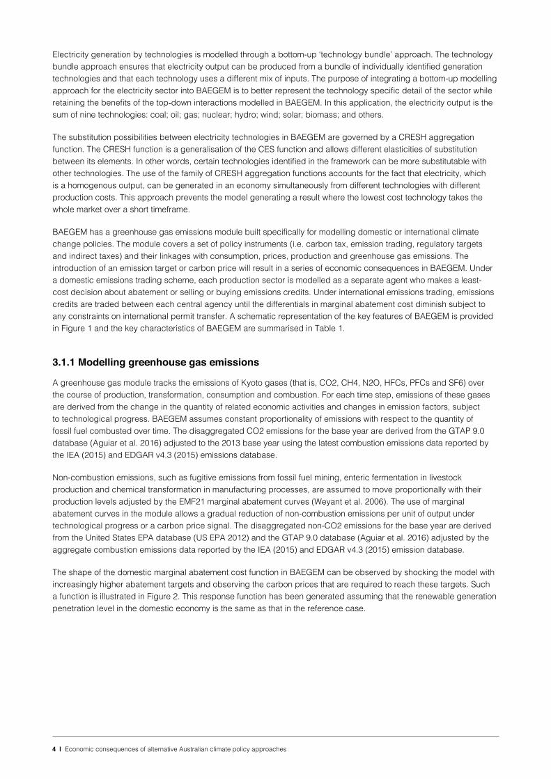
BAEGEM has a greenhouse gas emissions module built specifically for modelling domestic or international climate change policies. The module covers a set of policy instruments (i.e. carbon tax, emission trading, regulatory targets and indirect taxes) and their linkages with consumption, prices, production and greenhouse gas emissions. The introduction of an emission target or carbon price will result in a series of economic consequences in BAEGEM. Under a domestic emissions trading scheme, each production sector is modelled as a separate agent who makes a least-cost decision about abatement or selling or buying emissions credits. Under international emissions trading, emissions credits are traded between each central agency until the differentials in marginal abatement cost diminish subject to any constraints on international permit transfer. A schematic representation of the key features of BAEGEM is provided in Figure 1 and the key characteristics of BAEGEM are summarised in Table 1.

3.1.1 Modelling greenhouse gas emissions

A greenhouse gas module tracks the emissions of Kyoto gases (that is, CO2, CH4, N2O, HFCs, PFCs and SF6) over the course of production, transformation, consumption and combustion. For each time step, emissions of these gases are derived from the change in the quantity of related economic activities and changes in emission factors, subject to technological progress. BAEGEM assumes constant proportionality of emissions with respect to the quantity of fossil fuel combusted over time. The disaggregated CO2 emissions for the base year are derived from the GTAP 9.0 database (Aguiar et al. 2016) adjusted to the 2013 base year using the latest combustion emissions data reported by the IEA (2015) and EDGAR v4.3 (2015) emissions database.

Non-combustion emissions, such as fugitive emissions from fossil fuel mining, enteric fermentation in livestock production and chemical transformation in manufacturing processes, are assumed to move proportionally with their production levels adjusted by the EMF21 marginal abatement curves (Weyant et al. 2006). The use of marginal abatement curves in the module allows a gradual reduction of non-combustion emissions per unit of output under technological progress or a carbon price signal. The disaggregated non-CO2 emissions for the base year are derived from the United States EPA database (US EPA 2012) and the GTAP 9.0 database (Aguiar et al. 2016) adjusted by the aggregate combustion emissions data reported by the IEA (2015) and EDGAR v4.3 (2015) emission database.

The shape of the domestic marginal abatement cost function in BAEGEM can be observed by shocking the model with increasingly higher abatement targets and observing the carbon prices that are required to reach these targets. Such a function is illustrated in Figure 2. This response function has been generated assuming that the renewable generation penetration level in the domestic economy is the same as that in the reference case.


Figure 1: A schematic diagram of BAEGEM

4. DatabaseThe BAEGEM2013 database is derived from several sources. At its core, the database is a global Social Accounting Matrix (SAM), which captures the flow of economic transactions of households, governments, producers and international transport operators. Key economic transactions such as private consumption, government consumption, investment, total exports and total imports are benchmarked with the latest 2013 data from the United Nations (UN 2015) and the International Monetary Fund (IMF 2016). The industry structure for each economy is derived from the GTAP v9 database. For Australia, the SAM is supplemented by the use of industry gross-value data and industry import and export data from the Australian Bureau of Statistics.

In addition to the SAM, BAEGEM2013 incorporates energy data and electricity generation data from IEA publications (IEA 2015). Australian emissions for 2013 are based on Australian Department of Environment and Energy (2018). International emissions in BAEGEM2013 are derived from the GTAP 9 database (Aguiar et al 2016), the IEA CO2 emission database (2014) and the EDGAR v4.3 (2015) database.


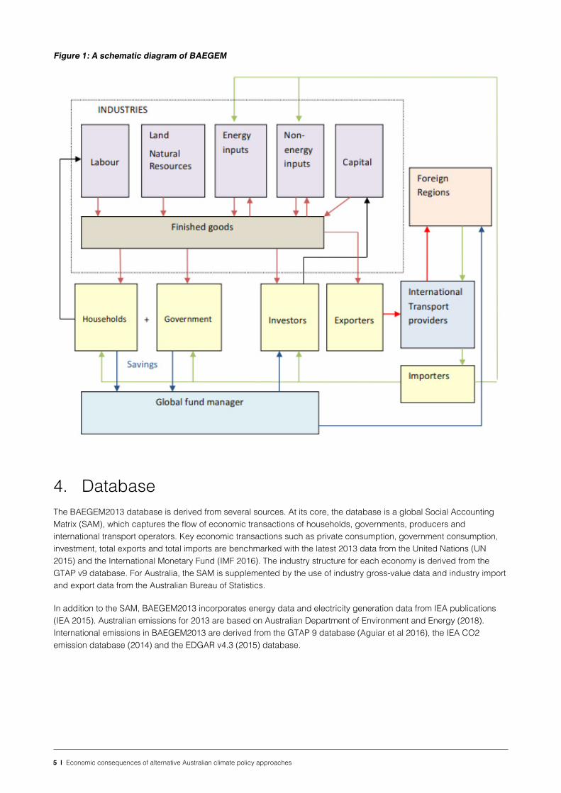
Table 1: Overview of BAEGEM

DISTINGUISHING FEATURE BAEGEM

Solution Concept Market equilibrium driven by supply and demand

Expectations/Foresight Recursive dynamics

Representation of the world economy

For the purposes of the present paper the world is divided into 18 economies as shown in Table 2

Representation of end-use sectors

There is one representative household and one government for each economy

Investment dynamics Investment is driven by long-term GDP growth rates and investment return differentials between economies

Labour market flexibility Not fully flexible, lower GDP growth rate will a trigger higher unemployment rate and a fall in real wages

Link between energy system and macro-economy

GDP sets the scale of economic activity in the model, which in turn drives the demand for each commodity in each segment of the world economy

Greenhouse gases covered CO2, CH4, N2O, HFCs, PFCs and SF6

Emission sectors covered Energy, Transport, Fugitives, Industry, Agriculture, Waste, LULUCF

Electricity production Substitution allowed between coal, gas, oil, hydro, nuclear, wind, solar, biomass and other renewables

Technological Change/Learning

Learning-by-doing gradually reduces the average production costs of renewable technologies (except hydro), compared with conventional electricity technologies

Integration costs Increased investment in intermittent renewable electricity technologies incurs additional capital integration costs to firm generation from these sources. Firming costs are based on estimates in Lovegrove et al. (2018).

Thermal efficiency improvement for fossil fuel electricity generation

0.5 per cent per year over the reference case

Energy consumption Substitution allowed between coal, gas, liquid fuel and electricity

Fuel consumption in transportation

Substitution allowed between coal, oil, gas, biofuel and electricity

Autonomous fuel efficiency improvement for transportation

2.5 per cent per year

Autonomous energy efficiency in other sectors

0.5 per cent for developed economies, 1 per cent for developing economies

Implementation of climate policy targets

Carbon prices, cap-and-trade, indirect taxes, regulatory targets, and combinations of the above


Figure 2: Australian domestic marginal abatement cost function in BAEGEM

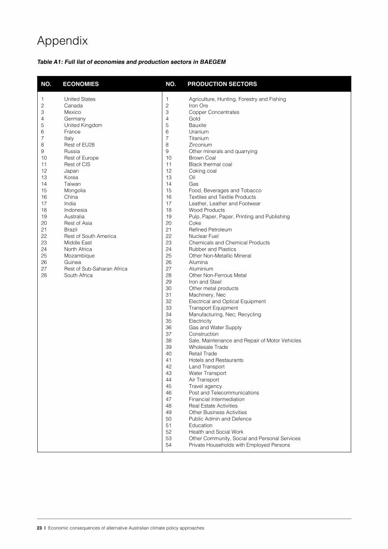
The full BAEGEM2013 database divides the world into 28 regions, and the database covers 54 commodity groups with a strong focus on energy and mineral commodities. It includes black thermal coal, brown coal, coking coal, oil, gas, iron ore, bauxite, copper, gold, uranium, titanium, zirconium and other minerals. Each production sector is assumed to produce a single, homogenous commodity within their regions. The full list of regions and production sectors is shown in Appendix Table A1. For this study, the database was aggregated to 18 regions and 21 sectors (Table 2).

5. Reference case and Policy ScenariosThe key objective in this paper is to evaluate the economic impacts of the domestic climate change policies proposed by the two main political parties in Australia. From this purpose, one reference case and six policy scenarios were specified.

5.1 Reference case

The reference case is a scenario representing the world in which current climate change mitigation policies continue to 2030 but where there is no new international agreement on mitigation targets from 2020. As such, before 2020, developed countries including Australia implement measures to reach their pledged 2020 emission targets. Developing countries continue their existing mitigation policies but do not aim to meet any quantitative emission reduction targets.

Population growth, economic growth, energy efficiency improvements and non-combustion emissions improvements are some of the most important determinants of reference case emissions projections. Under the current reference case, the population in Australia is assumed reach 28.5 million by 2030. Assumptions on population growth to 2030 in other key countries and regions are provided in Table 3. These growth rates are consistent with the medium variant projections in the United Nations’ World Population Prospects (UN 2015).

Australia’s real GDP is assumed to grow on average at 2.91 per cent over the projection period to 2030, slightly below its twenty-year long-term trend rate. Economic growth rate assumptions for the other key countries and regions in BAEGEM are also documented in Table 3. These growth rates are based around forecasts by the International Monetary Fund (IMF 2016).

The reference case assumes that thermal efficiency for fossil fuel electricity generation will improve by 0.5 per cent a year until 2030. Hence, for every gigawatt-hour of electricity generated from fossil fuel plant, 0.5 per cent less fossil fuel is consumed each year across the average of existing and new plant.


Autonomous fuel efficiency in transportation improves by 2.5 per cent a year until 2030. For land transportation, this improvement applies to each vehicle type. Fleet-wide fuel efficiency improvements resulting from substitution between different types of vehicles are modelled separately in BAEGEM and any improvements from this effect are additive with autonomous fuel efficiency improvements.

Energy efficiency in other uses improves by 0.5 per cent a year in developed countries and 1.0 per cent a year in developing countries. That is, for every unit of output, less energy is required to produce the same level of output every year. However, energy efficiency improvement does not necessarily imply lower energy consumption or lower emissions. Energy efficiency improvements could stimulate consumption through cost reduction and thus increase energy consumption.

Non-combustion emissions per unit of output have been falling over time due to technological advancement and better management practices. BAEGEM assumes these trends will continue with non-combustion emissions improving by 1.5 per cent a year per unit of output under the reference case.

Table 2: Regions and sectors in BAEGEM

REGIONS SECTORS

1 United States 1 Crops

2 Canada 2 Livestock

3 Mexico 3 Forestry

4 EU27 4 Fishing

5 Russia 5 Thermal Coal

6 Rest of Europe 6 Metallurgical Coal

7 China 7 Oil and Gas

8 India 8 Oil refinery

9 Japan 9 Iron ore

10 Korea 10 Other mining

11 Australia 11 Food processing

12 Rest of Asia 12 Chemicals, rubber and plastics

13 Brazil 13 Manufacture of non-metallic mining products

14 Rest of Latin America 14 Other manufacturing

15 Middle East 15 Iron and Steel

16 North Africa 16 Non-Ferrous Metal

17 South Africa 17 Electricity

18 Rest of Africa 18 Construction

19 Land Transport

20 Air and water Transport

21 Services

Australia’s real GDP is assumed to grow on average at 2.91 per cent over the projection period to 2030, slightly below its twenty-year long-term trend rate. Economic growth rate assumptions for the other key countries and regions in BAEGEM are also documented in Table 3. These growth rates are based around forecasts by the International Monetary Fund (IMF 2016).

The reference case assumes that thermal efficiency for fossil fuel electricity generation will improve by 0.5 per cent a year until 2030. Hence, for every gigawatt-hour of electricity generated from fossil fuel plant, 0.5 per cent less fossil fuel is consumed each year across the average of existing and new plant.


Autonomous fuel efficiency in transportation improves by 2.5 per cent a year until 2030. For land transportation, this improvement applies to each vehicle type. Fleet-wide fuel efficiency improvements resulting from substitution between different types of vehicles are modelled separately in BAEGEM and any improvements from this effect are additive with autonomous fuel efficiency improvements.

Energy efficiency in other uses improves by 0.5 per cent a year in developed countries and 1.0 per cent a year in developing countries. That is, for every unit of output, less energy is required to produce the same level of output every year. However, energy efficiency improvement does not necessarily imply lower energy consumption or lower emissions. Energy efficiency improvements could stimulate consumption through cost reduction and thus increase energy consumption.

Non-combustion emissions per unit of output have been falling over time due to technological advancement and better management practices. BAEGEM assumes these trends will continue with non-combustion emissions improving by 1.5 per cent a year per unit of output under the reference case.

Table 3: Population and economic growth assumptions (% average per year), reference case

POPULATION GROWTH, % REAL GDP GROWTH, %

2016-2020 2021-2030 2016-2020 2021-2030

United States 0.71 0.68 2.24 1.95

Canada 0.90 0.77 2.00 2.00

Mexico 1.24 0.98 2.84 3.34

EU27 0.13 0.03 1.80 1.50

Russia -0.01 -0.23 1.20 2.20

Rest of Europe 0.82 0.42 2.67 2.88

China 0.39 0.12 5.81 4.94

India 1.11 0.90 7.62 6.31

Japan -0.23 -0.40 0.43 0.96

Korea 0.36 0.23 3.01 2.91

Australia 1.31 1.06 2.94 2.91

Rest of Asia 1.23 1.02 5.02 5.02

Brazil 0.76 0.53 1.25 2.90

Rest of Latin America 1.06 0.87 2.47 4.00

Middle East 1.71 1.50 3.02 3.64

North Africa 1.81 1.51 4.31 4.42

South Africa 1.21 0.94 2.02 3.32

Rest of Africa 2.77 2.60 4.77 5.30

Australian reference case emissions are calibrated to the Australian Government’s most recent emissions projections to 2030 by emissions sector (Department of Environment and Energy 2018). For Australia, total emissions in the reference case are assumed to reach 540 Mt CO2e by 2020. Existing climate change mitigation policies including the Emission Reduction Fund (ERF), the Renewable Energy Target (RET) scheme, and the National Carbon Offset Standard (NCOS) are fully reflected in the reference case. In the case of the RET a target of 33 000 GWh is set for the large scale scheme by 2020 with the legislation and target remaining in place until 2030. No new policy measures are introduced in the reference case after 2020. Australian emissions are calibrated to reach 563 Mt CO2e in 2030 consistent with the latest Australian Government projections.


5.2 Policy scenarios

The policy scenarios were defined by varying assumptions on abatement targets, renewable energy generation shares and access to international permits to meet part of the domestic mitigation task. The scenarios are summarised in Table 4.

Scenarios 1 – 3 impose an emission target representing a 27 per cent reduction off 2005 levels consistent with the current federal government’s announced Paris contribution of a reduction in emissions to 26 to 28 per cent by 2030. Scenarios 4 – 6 impose a more stringent emissions target representing a reduction of 45 per cent compared to 2005 levels. These different targets were chosen to reflect the publicly announced emissions targets of the Coalition and Labor parties respectively.

To reflect a further ambition of the Labor party, a renewable energy generation target of 50 per cent by 2030 applies to scenarios 4 – 6. For Scenarios 1 – 3 the renewable target remains close to the reference case at around 36 per cent by 2030. This level is consistent with the renewable electricity generation share implied by the projections presented in Department of Environment and Energy (2018).

It is assumed that emissions reductions are applied linearly from 2020 to ensure that the specified target is met in 2030 and that all Australian domestic sectors contribute to the emissions reductions task. In scenarios 2,3,5 and 6, where the Kyoto carryover is available to meet the Paris target, the carryover projection is taken from Department of Environment and Energy (2018).

International permit trading is allowed in scenarios 3 and 6, where it is assumed that up to 25 per cent of the target can be met by the purchase of emissions permits from overseas at the world permit price. To calculate the world permit price, it is assumed that all countries with NDCs under the Paris Agreement fully meet those commitments by the years specified in their individual NDCs. Further, it is assumed that the United States reaches its NDC whether it remains as a member of the Paris Agreement or not. These scenarios have been included to provide context to the potential implications of international trade in permits for contributing to escalating emissions targets versus attempts to meet targets solely within Australia’s borders. These scenarios reflect any trade effects resulting from Australia and other countries meeting their respective Paris commitments together.

Table 4: Policy scenarios assumption summary

SCENARIO EMISSIONS ASSUMPTIONS

Reference case Without new policy beyond 2020 and Australian emissions calibrated to 2018 DEE projections

Scenario 1: -27% from 2005 by 2030

Scenario 2: -27% from 2005 by 2030 with use of Kyoto carryover

Scenario 3: -27% from 2005 by 2030 with use of carryover and permit trading

Scenario 4: -45% from 2005 by 2030 and 50% renewables

Scenario 5: -45% from 2005 by 2030 and 50% renewables with use of carryover

Scenario 6: -45% from 2005 by 2030 and 50% renewables with carryover and trading

Emissions trading allows industries with higher marginal abatement costs to purchase emissions permits from industries with lower marginal abatement costs. As such, the overall abatement cost for the economy is reduced as industries search for least cost alternatives to meet the regulatory target. The price paid by one industry to another industry for compensating their effort to reduce one extra tonne of CO2 equivalent is the market price for carbon. This market-based carbon price is explicitly modelled in BAEGEM with the expectation that the more stringent the emission target, the higher the carbon price (all else equal).

Emissions trading in BAEGEM is represented at the industry level. The marginal abatement cost curve of each industry reflects the aggregate effect of individual firms in the industry. For each time step, BAEGEM compares the marginal


abatement cost of each industry with respect to the prevailing carbon price and gives an approximation of the least cost solution. The least cost solution is influenced by a number of factors in each industry including: (i) fuel uses; (ii) ease of fuel substitution; (iii) emissions sources; (iv) emissions intensity; (v) output level; (vi) ease of output substitution; and (vii) costs of alternative technologies.

The likely costs of green technologies over the coming decade have a strong influence on intertemporal abatement costs. This is of particular significance in the electricity and transport sectors. BAEGEM assumes that that the intermittency of wind and solar energy does not put cost pressure on the power system until the share of electricity generation from intermittent renewables reaches 20 per cent. Beyond this threshold, the power system requires dispatchable power plants on standby, or sufficient installed battery or other storage to meet any sudden deficit in electricity supply. It is assumed that the existing reliability standards in the domestic electricity markets are maintained.

BAEGEM assumes that intermittency costs gradually increase from zero to $45/MWh when the share of generation from wind and solar increases from 20 per cent to 35 per cent. The intermittency and integration costs are assumed to peak at $200/MWh when the share of generation from wind and solar exceeds 75 per cent.

Population growth rates in the policy scenarios are the same as those in the reference case but real GDP growth rates are determined by the model in the policy scenarios. The labour market is not fully flexible, so unemployment can vary in the short to medium term. Depending on the size of the policy shock it is assumed that between 15 and 30 per cent of the adjustment in the labour market is represented by a fall in employment and the remainder is represented by a fall in real wages.

6. ResultsIn this section the results of modelling the scenarios described above in BAEGEM are described. The simulation results are discussed with a focus on the impacts on emissions, GDP, GNP, the electricity market, sectoral output, employment and real wages. The results reflect the economic impacts of the scenarios relative to what otherwise would have occurred if no policy interventions were implemented. They also describe the incremental effects of adding flexibility to the method by which emissions abatement targets are reached. All prices are expressed in real 2016$A unless otherwise stated.

6.1 Emissions reductions and carbon penalties

Australian emissions are projected to reach 563Mt CO2e by 2030 under the reference case. The greatest abatement under the policy scenarios is achieved by Labor’s proposed 45 per cent reduction policy excluding permit trading or carry-over, which results in 333Mt CO2e of emissions by 2030.

Emissions under all other scenarios fall within this range, with domestic emissions higher under scenarios that allow the greatest flexibility in meeting domestic targets. This reflects firstly that the Kyoto carry-over represents an intertemporal transfer from the past that lowers the emissions reduction effort required in the projection period, while scenarios that allow permit trading imbed a lower domestic abatement task via a partial contribution from international emissions reductions (where they can be done more cost effectively than in Australia). The domestic emissions outcomes under each scenario are shown in Figure 3.

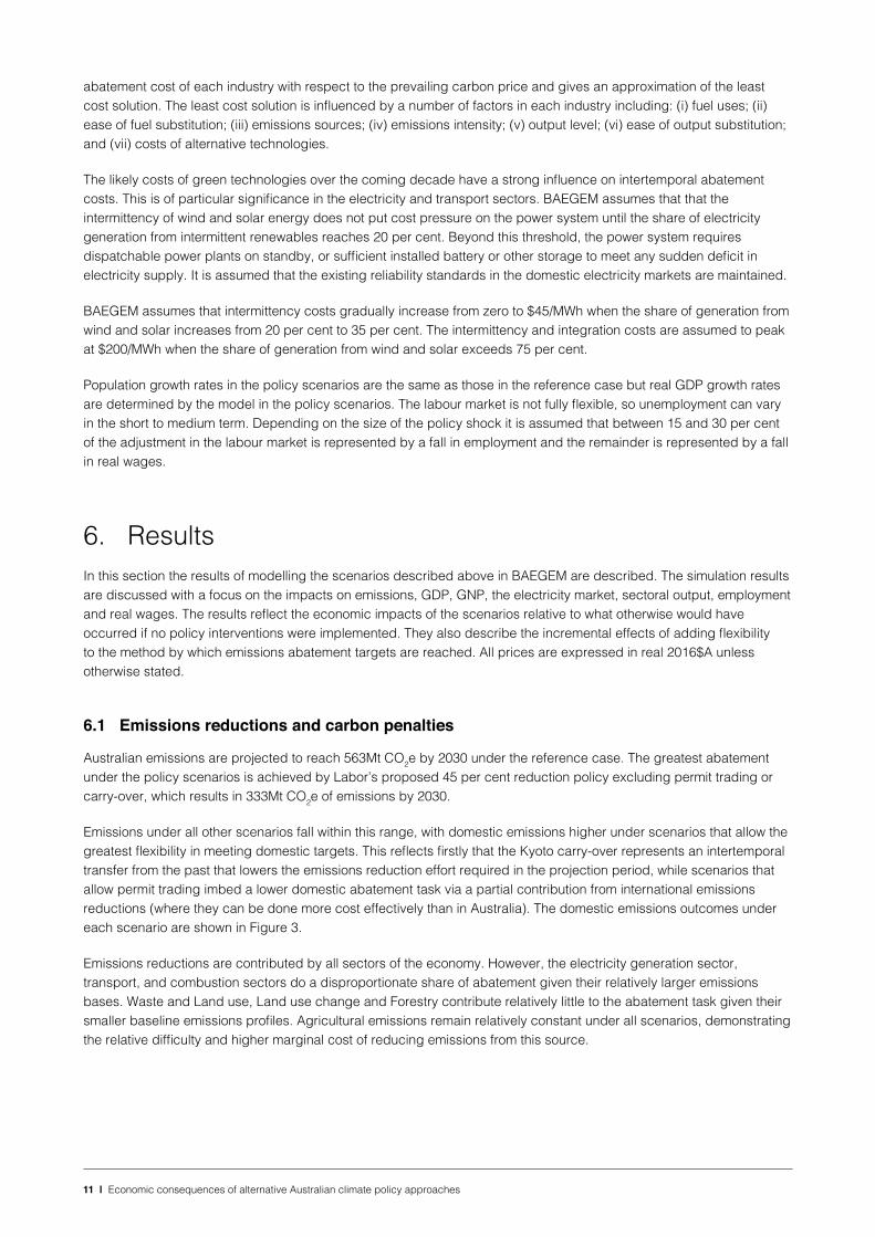
Emissions reductions are contributed by all sectors of the economy. However, the electricity generation sector, transport, and combustion sectors do a disproportionate share of abatement given their relatively larger emissions bases. Waste and Land use, Land use change and Forestry contribute relatively little to the abatement task given their smaller baseline emissions profiles. Agricultural emissions remain relatively constant under all scenarios, demonstrating the relative difficulty and higher marginal cost of reducing emissions from this source.


Emissions reductions are contributed by all sectors of the economy. However, the electricity generation sector, transport, and combustion sectors do a disproportionate share of abatement given their relatively larger emissions bases. Waste and Land use, Land use change and Forestry contribute relatively little to the abatement task given their smaller baseline emissions profiles. Agricultural emissions remain relatively constant under all scenarios, demonstrating the relative difficulty and higher marginal cost of reducing emissions from this source.

Figure 3: Australia’s domestic greenhouse gas emissions, reference case and policy scenarios

The economic impacts associated with emissions abatement result from the introduction of either an explicit or a shadow carbon price. The two main factors that influence the carbon price are the magnitude of the emissions abatement task and the availability and cost of abatement options.

Where international trade in emissions permits occurs, this lowers the marginal abatement cost by opening up new opportunities for lower cost emissions reduction from other countries, thereby lowering the Australian carbon price and ameliorating the economic effects of the penalty. The projected international carbon price in 2030 is $US42/t CO2e.

This dynamic clearly plays out in the estimated shadow carbon penalties for Australia under the modelled scenarios (Table 5). The Coalition’s emissions target of -27 per cent below 2005 levels by 2030 results in an estimated shadow carbon price of A$263/t CO2e in 2030. Allowing for both Kyoto carry-over and international trade in emissions permits reduces the carbon penalty to $73/t CO2e.

Labor’s 45 per cent emissions target over the same time horizon imposes a shadow carbon penalty of A$696/tCO2e, which can again be substantially reduced to $97/t CO2e by allowing for emissions reduction carry-over between commitment periods and international permit trading.

There is no suggestion here that future governments will impose a carbon tax as such. Both major political parties have already announced some policies aimed at reducing emissions and none of these alternatives involve direct taxation of carbon emissions. However, all of these policies impose a cost on the economy and the carbon penalty reported here is one proxy for that cost.3

Table 5: Carbon price, $A/tCO2e in 2030

YEAR SCENARIO 1 SCENARIO 2 SCENARIO 3 SCENARIO 4 SCENARIO 5 SCENARIO 6

Carbon price 263 92 73 696 326 97

3 Comparing the economic costs of different abatement policies is a complex task. For a discussion of possible methodology and some estimates see Productivity Commission (2011).


6.2 Gross Domestic Product

Real GDP is the most commonly used measure of the overall performance of an economy. The modelling indicates that any form of climate policy will have a negative impact on GDP relative to the reference case, with GDP losses ranging from A$17 billion to A$432 billion in 2030 (see Figure 4). GDP growth is affected least where there is flexibility in achieving emissions targets. This flexibility is modelled here via Kyoto carry-over of emissions reductions surplus to those required to meet Australia’s Kyoto 2nd commitment period pledge, and international trade in permits up to the specified limit.

Under the Coalition emissions target of -27 per cent by 2030, if carry-over and permit trading are allowed, Australia’s GDP growth rate over the period from 2021 to 2030 is projected to slow very moderately by around 0.1 percentage points per year from a reference case annual growth rate of 2.91 per cent.

Under Labor’s modelled policy scenarios, a similar dynamic is at play where less flexibility in the approach to emissions reduction results in increasingly negative effects on GDP. However, when the emissions reduction ambition is set higher (to -45 per cent by 2030), the relative economic growth effects resulting from less flexible policy are magnified. The projected annual GDP growth rate over the period between 2021 and 2030 slows to 2.65 per cent where flexible instruments are deployed and t0 0.88 per cent where they are not. The cumulative impact of slower growth over the period to 2030 results in projected GDP losses of $228 billion when permit trading and use of the carry-over is allowed. The cumulative loss is projected to be $1.2 trillion without either carry-over or permit trading.4

Figure 4: Real GDP deviation from the reference case, 2030

6.3 Gross National Product

In BAEGEM, the sale and purchase of emissions permits between economies are considered as international transfers of capital income and as such are reflected in the calculation of Gross National Product (GNP). An economy that mainly purchases emissions permits from other economies would expect its GNP to fall relative to its GDP while an economy that mainly sells emissions permits would expect its GNP to rise relative to its GDP, all other factors held constant.

4 The cumulative losses in GDP are expressed in $A 2016 calculated at an assumed social discount rate of 2.6 per cent.


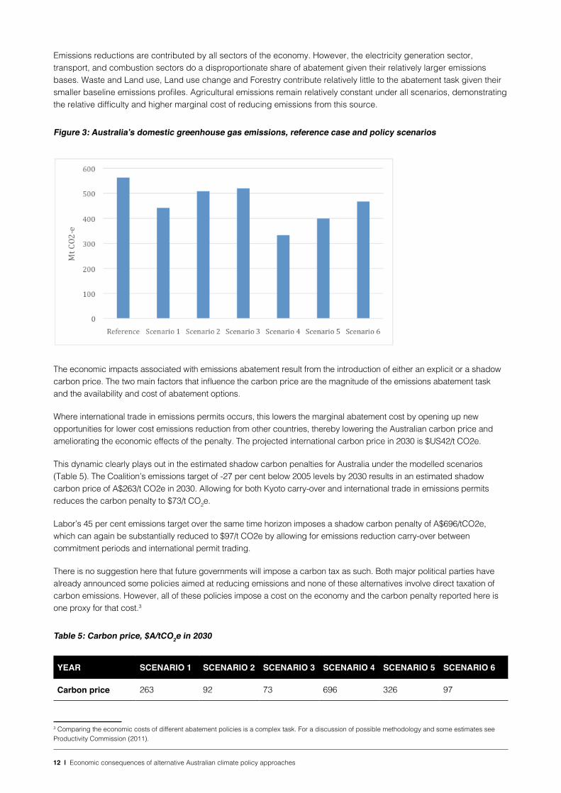
The projected net present value (NPV) of the loss of GNP over the decade from 2021-2030, relative to the reference case, ranges from $80 billion (scenario 3) to $1.2 trillion (scenario 4) under the modelled Coalition and Labor policy scenarios respectively (see Table 5). Consistent with the projected impacts on GDP the results suggest that the more policy flexibility that is allowed the less the negative impacts of the reductions in emissions on GNP.

Table 5: NPV* of cumulative real GNP loss from 2021-2030, relative to the reference case

YEAR SCENARIO 1 SCENARIO 2 SCENARIO 3 SCENARIO 4 SCENARIO 5 SCENARIO 6

Real GNP ($b) -$293 -$89 -$80 -$1237 -$502 -$254

*Applied with a social discount rate of 2.6 per cent a year

6.4 Electricity market

Under the reference case, electricity generation in Australia is projected to reach around 300 TWh by 2030. This is equivalent to a growth rate from 2021 to 2030 of around 1.6 per cent a year, accompanied by projected higher consumption by electric vehicles. The share of renewable energy, including hydro-electricity, is projected to increase from around 13 per cent in 2013 to around 36 per cent by 2030 in the reference case. Total electricity demand is lower under each of the policy scenarios modelled than under the reference case.

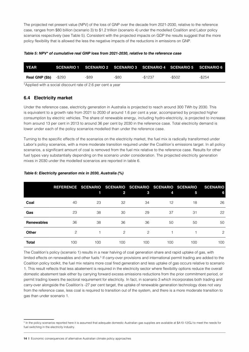
Turning to the specific effects of the scenarios on the electricity market, the fuel mix is radically transformed under Labor’s policy scenarios, with a more moderate transition required under the Coalition’s emissions target. In all policy scenarios, a significant amount of coal is removed from the fuel mix relative to the reference case. Results for other fuel types vary substantially depending on the scenario under consideration. The projected electricity generation mixes in 2030 under the modelled scenarios are reported in table 6.

Table 6: Electricity generation mix in 2030, Australia (%)

REFERENCE SCENARIO 1

SCENARIO 2

SCENARIO 3

SCENARIO 4

SCENARIO 5

SCENARIO 6

Coal 40 23 32 34 12 18 26

Gas 23 38 30 29 37 31 22

Renewables 36 38 36 36 50 50 50

Other 2 1 2 2 1 1 2

Total 100 100 100 100 100 100 100

The Coalition’s policy (scenario 1) results in a near halving of coal generation share and rapid uptake of gas, with limited effects on renewables and other fuels.5 If carry-over provisions and international permit trading are added to the Coalition policy toolkit, the fuel mix retains more coal fired generation and less uptake of gas occurs relative to scenario 1. This result reflects that less abatement is required in the electricity sector where flexibility options reduce the overall domestic abatement task either by carrying forward excess emissions reductions from the prior commitment period, or permit trading lowers the sectoral requirement for electricity. In fact, in scenario 3 which incorporates both trading and carry-over alongside the Coalition’s -27 per cent target, the uptake of renewable generation technology does not vary from the reference case, less coal is required to transition out of the system, and there is a more moderate transition to gas than under scenario 1.

5 In the policy scenarios reported here it is assumed that adequate domestic Australian gas supplies are available at $A10-12/GJ to meet the needs for fuel switching in the electricity industry.


At the higher emissions abatement task of -45 per cent proposed by Labor, the fuel mix must radically transform. Around three-quarters of reference case coal fired generation must retire by 2030, and renewables penetration must rise relative to reference case uptake. Gas penetration increases 14 percentage points beyond reference case levels in similar proportion to the contribution of gas under the Coalition policy scenario, noting however that overall electricity demand is lower under scenarios 4 – 6 compared with scenarios 1 – 3. Again, carry-over allowances and permit trading reduce the size of the task, thereby mitigating the extent of electricity sector transformation. However, given Labor’s fixed policy objective of a 50 per cent renewables target, much greater transition away from coal is observed than under the equivalent Coalition policy combinations. The transition to gas remains significant under the Labor policies modelled, making up a major share of the fuel mix in combination with renewables. In all the modelled scenarios the projected high gas penetration is critically dependent on the assumption that sufficient domestic gas supply is available.

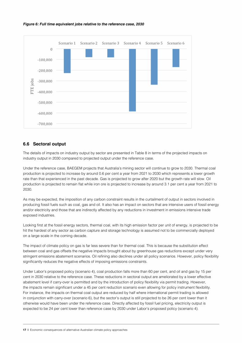
As expected, the effects on wholesale electricity prices are non-trivial, with the largest single determinant being abatement ambition, followed by the level of policy flexibility. The wholesale price reflects the LCOE of the existing generation capacity, the intermittency and integration costs of wind and solar technologies, and the supply and demand for electricity. Any policy instruments targeting greenhouse gas emissions in the electricity generation sector will have a direct impact on the wholesale price. On the other hand, the direct effect on the price paid for transmission, distribution and retail services will be small because emissions from these activities are small.

Under the reference case the wholesale electricity price in Australia is projected to increase from $69/MWh in 2016 to around $81/MWh by 2030. This represents an increase of about 1.5 per cent a year in real terms. For comparison, the GSP weighted average wholesale price in the National Electricity Market (NEM) from 2005-2016 rose about 3.2 per cent a year in nominal terms. The low growth in the wholesale electricity price throughout the projection period reflects the low LCOE of the existing generation capacity with limited further depreciation value and the rising competition from renewable energy.

The wholesale electricity price is projected to rise much faster under the policy scenarios. A rise in the shadow carbon price, increases in average LCOE after switching to new-build renewables and gas and increases in intermittency costs are the key factors driving the wholesale electricity price higher in the policy scenarios. By 2030, Australian electricity prices are projected to increase around 38 per cent under the Coalition policy and by 94 per cent under Labor’s proposed policy, relative to the reference case electricity price projection. These effects can be mitigated by more than two-thirds by allowing carry-over of emissions and permit trading.

Given Australia’s electricity prices are already high relative to international standards, these price effects translate into significant consequences for industrial activity, and hence real wages and employment. The modelled wholesale electricity price projections at 2030 are presented in Table 7.

Table 7: Impacts on wholesale electricity price in Australia in 2030, $/MWh

Reference Scenario 1 -27%

Scenario 2 -27% w c/o

Scenario 3 -27% w c/o & trade

Scenario 4 -45%

Scenario 5 -45% w c/o

Scenario 6 -45% w c/o & trade

Wholesale electricity price ($/MWh)

81 112 93 91 157 128 111

6.5 Employment and wages

BAEGEM assumes that the labour market is neither fully flexible nor fully sticky under the policy scenarios. That is, real wages fall following the implementation of emission targets but do not fall to a level that would hold the unemployment rate at the non-accelerating inflation rate of unemployment (NAIRU). Here, BAEGEM assumes that the adjustment in real wages and employment are bounded by the adjustment in real GDP in percentage terms. The actual outcomes in the labour market will ultimately depend not only on the government’s emission reduction policies but also on its labour market policies.


Under the reference case, real wages in Australia are projected to increase by 1.95 per cent a year during the next decade. In the policy scenarios, reflective of significant reductions in output across most sectors of the Australian economy, real wages are projected to fall compared to what they would otherwise have been (Figure 5). The larger the emissions reduction by 2030, and therefore the higher the implicit carbon price, the lower the real wage rate. The full-time adult equivalent average real wage in 2030 is projected to be around $106 000 under the reference case. Under scenario 1 real wages are projected to be around $101 000 in 2030. The projected fall in real wages under scenarios 2 and 3 compared to the reference case is more moderate at around $105 000. Under scenario 4 real wages are projected to be around $82 000 in 2030, 23 per cent below the reference case level. The negative impact on real wages is significantly moderated with policy flexibility under scenarios 5 and 6. In those scenarios projected real wages in 2030 are around $97 000 and $103 000 respectively.

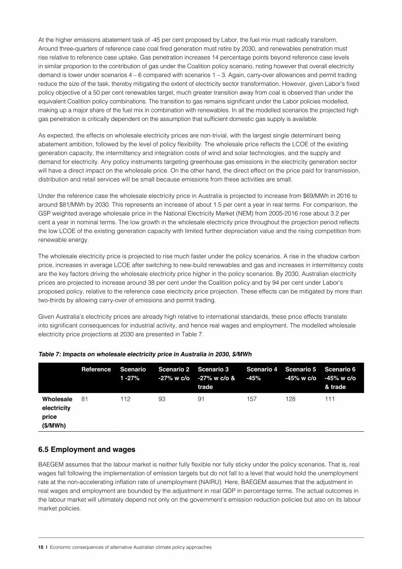
Job losses relative to reference case employment in 2030 are significant – ranging from -227,000 under the Coalition target and rising to -586,000 under the proposed Labor policy. Allowing Kyoto carry-over and permit trading to contribute 25 per cent of the target mitigates these projected job losses significantly (Figure 6). The impact on employment is not expected to be evenly spread across sectors. It can be expected that the greatest negative effects will be felt in sectors such as coal production and the regions in which this sector is located. Burke, Best and Jotzo (2019) explore some of these adjustment effects in the coal-fired power sector.

Figure 5: Australia’s real wage relative to the reference case, 2030


Figure 6: Full time equivalent jobs relative to the reference case, 2030

6.6 Sectoral output

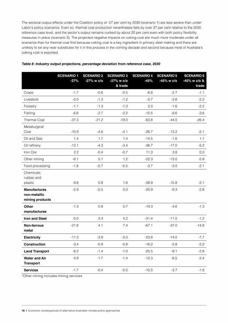
The details of impacts on industry output by sector are presented in Table 8 in terms of the projected impacts on industry output in 2030 compared to projected output under the reference case.

Under the reference case, BAEGEM projects that Australia’s mining sector will continue to grow to 2030. Thermal coal production is projected to increase by around 0.6 per cent a year from 2021 to 2030 which represents a lower growth rate than that experienced in the past decade. Gas is projected to grow after 2020 but the growth rate will slow. Oil production is projected to remain flat while iron ore is projected to increase by around 3.1 per cent a year from 2021 to 2030.

As may be expected, the imposition of any carbon constraint results in the curtailment of output in sectors involved in producing fossil fuels such as coal, gas and oil. It also has an impact on sectors that are intensive users of fossil energy and/or electricity and those that are indirectly affected by any reductions in investment in emissions intensive trade exposed industries.

Looking first at the fossil energy sectors, thermal coal, with its high emission factor per unit of energy, is projected to be hit the hardest of any sector as carbon capture and storage technology is assumed not to be commercially deployed on a large scale in the coming decade.

The impact of climate policy on gas is far less severe than for thermal coal. This is because the substitution effect between coal and gas offsets the negative impacts brought about by greenhouse gas reductions except under very stringent emissions abatement scenarios. Oil refining also declines under all policy scenarios. However, policy flexibility significantly reduces the negative effects of imposing emissions constraints.

Under Labor’s proposed policy (scenario 4), coal production falls more than 60 per cent, and oil and gas by 15 per cent in 2030 relative to the reference case. These reductions in sectoral output are ameliorated by a lower effective abatement level if carry-over is permitted and by the introduction of policy flexibility via permit trading. However, the impacts remain significant under a 45 per cent reduction scenario even allowing for policy instrument flexibility. For instance, the impacts on thermal coal output are reduced by half where international permit trading is allowed in conjunction with carry-over (scenario 6), but the sector’s output is still projected to be 26 per cent lower than it otherwise would have been under the reference case. Directly affected by fossil fuel pricing, electricity output is expected to be 24 per cent lower than reference case by 2030 under Labor’s proposed policy (scenario 4).


The sectoral output effects under the Coalition policy of -27 per cent by 2030 (scenario 1) are less severe than under Labor’s policy scenarios. Even so, thermal coal production nevertheless falls by over 37 per cent relative to the 2030 reference case level, and the sector’s output remains curbed by about 20 per cent even with both policy flexibility measures in place (scenario 3). The projected negative impacts on coking coal are much more moderate under all scenarios than for thermal coal first because coking coal is a key ingredient in primary steel making and there are unlikely to be any near substitutes for it in this process in the coming decade and second because most of Australia’s coking coal is exported.

Table 8: Industry output projections, percentage deviation from reference case, 2030

SCENARIO 1 -27%

SCENARIO 2 -27% w c/o


& trade

SCENARIO 4 -45%


SCENARIO 6 -45% w c/o &

trade

Crops -1.7 -0.6 -0.5 -6.8 -2.7 -1.1

Livestock -2.0 -1.3 -1.2 -0.7 -2.6 -2.2

Forestry -1.1 -1.3 -1.3 2.0 -1.6 -2.2

Fishing -6.6 -2.7 -2.2 -15.5 -8.6 -3.6

Thermal Coal -37.3 -21.2 -19.0 -63.8 -44.0 -26.4

Metallurgical Coal -10.9 -4.8 -4.1 -26.7 -13.2 -5.1

Oil and Gas 1.4 1.7 1.4 -14.5 -1.6 1.1

Oil refinery -13.1 -4.3 -3.4 -36.7 -17.0 -5.2

Iron Ore 2.2 -0.4 -0.7 11.3 3.8 0.3

Other mining -8.1 0.1 1.2 -22.3 -13.0 -5.9

Food processing -1.8 -0.7 -0.5 -3.7 -3.0 -2.1

Chemicals, rubber and plastic -9.8 0.8 1.8 -38.9 -15.8 -2.1

Manufactures non-metallic mining products

-5.9 -0.5 0.0 -20.9 -9.3 -2.8

Other manufactures

-1.3 0.8 0.7 -19.3 -4.6 -1.3

Iron and Steel -5.0 3.4 4.2 -31.4 -11.0 -1.2

Non-ferrous metal

-21.8 4.1 7.4 -67.1 -37.0 -14.8

Electricity -11.3 -3.9 -3.0 -23.8 -14.0 -7.7

Construction -3.4 -0.9 -0.8 -16.2 -5.8 -2.2

Land Transport -6.2 -1.4 -1.0 -20.5 -9.1 -2.8

Water and Air Transport

-4.9 -1.7 -1.4 -12.3 -6.5 -2.4

Services -1.7 -0.4 -0.5 -10.5 -3.7 -1.8*Other mining includes mining services


The oil and gas sector is positively affected under the Coalition’s modelled scenarios, with the substitution toward lower emissions-intensity gas a key factor in the outcome. Electricity output under scenario 1 declines 11 per cent by 2030 relative to the reference case, reducing to a 3 per cent curtailment by 2030 when policy flexibility is introduced in scenario 3.

Since fossil fuels underpin a substantive proportion of energy consumption in Australia both via electricity, direct and indirect use, the impacts of the climate policies modelled in this paper have broad ramifications beyond energy commodities and electricity. Cropping and fishing, manufacturing, construction, transport and services are all meaningfully affected.

Of note is the substantial transformation required in land-based transport to achieve these modelled climate policies. While the share of rail remains relatively constant between the reference case and policy scenarios, major shifts are observed out of internal combustion (ICE) and into hybrid and electric vehicles. This effect is most marked under the Labor policy scenario, where the ICE share falls from 73 per cent in 2030 under the reference case to 43 per cent, while hybrid and electric vehicle uptake rises from 4 per cent under the reference case to 32 per cent in scenario 4.

The energy intensive non-ferrous metals sector is heavily affected by the substantial curtailment of emissions and can be observed under most policy scenarios to be doing much of the heavy lifting alongside the coal and electricity sectors in reaching emissions targets. Under scenarios 2 and 3, non-ferrous metals output increases relative to the reference case because the sector benefits from policy flexibility and lower real wages.

Outputs of the manufacturing, transport and services sectors are also lower than reference case levels in response to increasingly stringent emissions abatement targets, reflecting energy cost pressures due to escalation of the implicit carbon price.

The iron ore industry is one of the few industries projected to experience a positive outcome under a range of scenarios. This is largely because the iron ore industry is not particularly emission-intensive relative to other sectors, is highly internationally competitive and would benefit from the projected reduction in real wages.

As shown in Table 8, other mining production is more negatively affected than iron ore, particularly under the Labor policy scenarios. This is because the industry is more emissions intensive than iron ore production, and electricity use in other mining is significantly higher.

7. Conclusions and Policy ImplicationsClimate and energy policy will almost certainly be a key differentiator between the two major political parties at the upcoming Australian Federal election. The Coalition government has proposed meeting Australia’s Paris Agreement commitments through a 26 – 28 per cent emissions reduction by 2030 relative to base-year emissions in 2005. The opposition Labor party has announced a higher emissions target of 45 per cent over the same time period, with an objective of 50 per cent renewable electricity generation and an aim to reach net zero emissions by mid-century.

This paper examines the economic impacts of adopting these different domestic emissions targets using the BAEGEM computable general equilibrium model. Six separate scenarios are modelled alongside a reference case scenario, which assumes no new policy beyond that already in place from 2020. Differentiating the scenarios are assumptions on emissions reductions, availability of mitigation through Kyoto carry-over, renewable energy targets and recognition of international emissions permits to meet part of the domestic mitigation task.

Cumulative GNP losses are estimated at A$293 billion by 2030 for the Coalition emissions reduction target of -27 per cent, and A$1.2 trillion under Labor’s higher 45 per cent emissions abatement goal. These GDP losses are brought about by the implicit carbon price and transition requirements for the economy to meet the emissions targets specified. A Coalition policy without policy flexibility leads to a shadow carbon price of A$263/tCO2e, while Labor’s proposed policy target incurs a projected carbon price of A$696/tCO2e.

Associated negative consequences for sectoral output, employment and wages are projected. The sectors hardest hit by the policies of both parties are electricity, thermal coal, non-ferrous mining and chemicals, rubber and plastic.


Policy flexibility in meeting emissions abatement targets is modelled via two options: i) by lowering the abatement task in the projection period by allowing carry-over of excess abatement from the Kyoto commitment period; and ii) by allowing part of the domestic abatement task to be met by international emissions permit trading. Both options are demonstrated to be important in ameliorating the adverse economic costs of reducing emissions. Results indicate that when these additional policy options are introduced, negative GNP effects are around one quarter of what they otherwise would be without policy flexibility. Of the two flexibility options examined in this paper, allowing Kyoto carry-over had a larger impact than enabling 25 per cent of the abatement task to be contributed by international permit trading.

In the present paper all sectors of the economy are assumed to participate in abatement activities with no exemptions applied. If some sectors were to be partially exempted from the abatement effort (and the targets remain the same) then additional burden would fall on the remaining sectors. For an ambitious target such as that represented by Labor policy, any special treatment of emissions intensive trade exposed industries would shift significant further burden directly onto households and the non-traded goods sectors. This issue is worthy of further analysis if proposals for special treatment of emissions intensive trade exposed industries emerge.

The emissions trading scheme modelled in this paper is efficient in the sense that emitters are allowed to buy and sell permits to ensure that the marginal tonne of abatement is done at the lowest possible cost in the domestic economy and that, subject to the restriction on purchasing overseas permits, permits generated in other countries can be used in Australia if it is cheaper to do so. Any form of emissions trading based on baseline and credit schemes will be less cost effective than the scheme reported here because there will inevitably be errors made in setting emissions baselines. In addition, any abatement achieved through regulation is likely to be less cost effective than the measures modelled here. It follows that the economic costs reported here may turn out to be an under-statement of the economic burden of the modelled scenarios on the Australian economy.

The paper highlights the significant economic consequences, and thereby the inherent political difficulties, associated with adoption of ambitious emissions reduction targets. It also demonstrates the sizeable benefits attached to building in adjunct policy measures that allow targets to be met flexibly, and at lowest marginal cost.


ReferencesAguiar, Angel, Badri Narayanan, & Robert McDougall, 2016. An Overview of the GTAP 9 Data Base, Journal of Global Economic Analysis, 1(1), 181-208.

Burke, P.J., Best, R. and Jotzo, F. 2019. ‘Closures of coal-fired power stations in Australia: local unemployment effects’, Australian Journal of Agricultural and Resource Economics, 63(1), 142-65.

Chan, G., Stavins, R. and Zou, J. 2018. ‘International climate change policy’, Annual Reviews of Resource Economics, 10, 335-60.

Department of the Environment 2016. ‘The Safeguard Mechanism – Overview’ https://www.environment.gov.au/system/files/resources/8fb34942-eb71-420a-b87a-3221c40b2d21/files/factsheet-safeguard-mechanism.pdf, 30 May 2016.

Department of Environment and Energy 2018. Australia’s emissions projections 2018, Commonwealth of Australia, http://www.environment.gov.au/system/files/resources/128ae060-ac07-4874-857e-dced2ca22347/files/australias-emissions-projections-2018.pdf (accessed December 2018).

EDGARv4.3 2015, European Commission, Joint Research Centre (JRC)/PBL Netherlands Environmental Assessment Agency. Emission Database for Global Atmospheric Research (EDGAR), release version 4.3.

Fisher, B.S. 2016. ‘Antipodean agricultural and resource economics at 60: climate change policy and energy transition’, Australian Journal of Agricultural and Resource Economics, 60(4), 692-705.

Fujimori, S., Su, X., Liu, J., Hasegawa, T., Takahashi, K., Masui, T. and Takimi, M. 2016a, ‘Implication of Paris Agreement in the context of long-term climate mitigation goals’, Springerplus 5(1): 1620.

Fujimori, S., Kubota, I., Dai, H., Takahashi, K., Hasegawa, T., Liu, J.Y., Hijioka, Y., Masui, T. and Takimi, M. 2016b. ‘Will international emissions trading help achieve the objectives of the Paris Agreement?’ Environmental Research Letters 11(10). https://iopscience.iop.org/article/10.1088/1748-9326/11/10/104001/meta.

Hanoch, G. 1971. ‘CRESH production functions’, Econometrica, 39(5), 695-712.

Hertel, T 1997. Global Trade Analysis: Modeling and Applications. Cambridge University Press, Cambridge.

IEA 2015. CO2 Emissions from Fuel Combustion, 2015 Edition. International Energy Agency, Paris.

IMF 2016. World Economic Database, April2016 Edition, International Monetary Fund.

Kompas, T., Pham, V.H. and Che, T.N. 2018. ‘The Effects of Climate Change on GDP by Country and the Global Economic Gains from Complying with the Paris Climate Accord’. Earth’s Future 6(8), 1153–1173. https://agupubs.onlinelibrary.wiley.com/doi/full/10.1029/2018EF000922.

Liu, W., McKibbin, W., Morris, A., Wilcoxen, P. 2019. ‘Global Economic and Environmental Outcomes of the Paris Agreement’, Brookings Institute, Climate and Energy Economics Discussion Paper, January 7, 2019.

Lovegrove, K., James, G., Leitch, D., Milczarek, A., Ngo, A. Rutovitz, J., Watt, M. and Wyder, J. 2018. Comparison of Dispatchable Renewable electricity Options: Technologies for an Orderly Transition, Report prepared for the Australian Renewable Energy Agency by the ITP Energised Group (ITP), Canberra.

McKibbin, W. 2016. ‘Comment 1 on ‘Climate change policy and energy transition’ by Fisher’, Australian Journal of Agricultural and Resource Economics, 60(4), 706-7.

Mi, R. and Fisher, B. S. 2014. Model Documentation: BAEGEM – the BAEconomics Computable General Equilibrium Model of the World Economy, http://www.baeconomics.com.au/wp-content/uploads/2014/02/BAEGEM-229 documentation-21Feb14.pdf).

Pant, H. 2007. GTEM: Global Trade and Environment Model. ABARE Technical report, Canberra.


Productivity Commission 2011. Carbon Emission Policies in Key Economies, Productivity Commission Research Report, Commonwealth of Australia, May.

United Nations 2015. National Accounts Statistics: Main Aggregates and Detailed Tables, United Nations Statistics Division.

United States Environmental Protection Authority 2012. Global Anthropogenic Non-CO2 Greenhouse Gas Emissions: 1990-2030, US EPA, viewed 24 April 2015, http://www.epa.gov/climatechange/Downloads/EPAactivities/EPA_Global_NonCO2_Projections_Dec2012.pdf.

Vandyck, T., Keramidas, K., Saveyn, B., Kitous, A. and Vrontisi, Z. 2016. ‘A global stocktake of the Paris pledges: implications for energy systems and economy’. Global Environmental Change 41 (2016): 46-63. https://ac.els-cdn.com/S095937801630142X/1-s2.0-S095937801630142X-main.pdf?_tid=37814930-82bb-43ad-b881-2f57723444c3&acdnat=1548647911_ad6cd63196c3afdbc507782e81bb2765

Weyant, J.P., de la Chesnaye, F.C. and Blanford, G.J. 2006. ‘Overview of EMF-21: multigas mitigation and climate policy’, The Energy Journal, Special Issue, 1-32.

Winchester, N. 2016. ‘Comment 2 on ‘Climate change policy and energy transition’ by Fisher’, Australian Journal of Agricultural and Resource Economics, 60(4), 708-9.

Woodland, A.D. 1976. ‘Modelling the production sector of an economy: a selective survey and analysis’, Working Paper No. 0-04, IMPACT of Demographic Change on Industry Structure in Australia papers, June 1976, http://www.copsmodels.com/opseries.htm.


AppendixTable A1: Full list of economies and production sectors in BAEGEM

NO. ECONOMIES NO. PRODUCTION SECTORS

1 United States 2 Canada 3 Mexico 4 Germany 5 United Kingdom6 France 7 Italy8 Rest of EU28 9 Russia 10 Rest of Europe 11 Rest of CIS 12 Japan 13 Korea 14 Taiwan 15 Mongolia 16 China 17 India 18 Indonesia 19 Australia 20 Rest of Asia 21 Brazil 22 Rest of South America 23 Middle East24 North Africa 25 Mozambique 26 Guinea 27 Rest of Sub-Saharan Africa 28 South Africa

1 Agriculture, Hunting, Forestry and Fishing2 Iron Ore3 Copper Concentrates4 Gold5 Bauxite6 Uranium7 Titanium8 Zirconium9 Other minerals and quarrying 10 Brown Coal11 Black thermal coal 12 Coking coal 13 Oil 14 Gas 15 Food, Beverages and Tobacco16 Textiles and Textile Products 17 Leather, Leather and Footwear 18 Wood Products 19 Pulp, Paper, Paper, Printing and Publishing 20 Coke 21 Refined Petroleum22 Nuclear Fuel23 Chemicals and Chemical Products 24 Rubber and Plastics 25 Other Non-Metallic Mineral26 Alumina 27 Aluminium 28 Other Non-Ferrous Metal 29 Iron and Steel 30 Other metal products 31 Machinery, Nec 32 Electrical and Optical Equipment 33 Transport Equipment 34 Manufacturing, Nec; Recycling 35 Electricity 36 Gas and Water Supply 37 Construction 38 Sale, Maintenance and Repair of Motor Vehicles 39 Wholesale Trade 40 Retail Trade 41 Hotels and Restaurants 42 Land Transport 43 Water Transport 44 Air Transport 45 Travel agency 46 Post and Telecommunications 47 Financial Intermediation 48 Real Estate Activities 49 Other Business Activities 50 Public Admin and Defence 51 Education 52 Health and Social Work 53 Other Community, Social and Personal Services54 Private Households with Employed Persons

Author: Brian S. Fisher Corresponding author: Brian Fisher ...€¦ · Corresponding author: Brian...

Documents

Transcript of Author: Brian S. Fisher Corresponding author: Brian Fisher ...€¦ · Corresponding author: Brian...