Australia's Low Pollution Future - The Short to Medium Run ...
47
The Short to medium Run Economic Costs of Alternative Emission Reduction Scenarios * Warwick J. McKibbin** Centre for Applied Macroeconomic Analysis in the ANU College of Business and Economics and The Brookings Institution and The Lowy Institute for International Policy Final Version 8 January 2009 * The views expressed in the paper are those of the authors and should not be interpreted as reflecting the views of any of the above collaborators or of the Institutions with which the authors are affiliated including the trustees, officers or other staff of the ANU, Lowy Institute or The Brookings Institution nor does it reflect the views of The Australian Treasury. This is a background paper prepared for the Australian Treasury report on “Australia’s Low Pollution Future: The Economics of Climate Change Mitigation”. Part of this research was jointly undertaken with Dr Alison Stegman and draws on joint research with Peter Wilcoxen. The authors thank Waranya Pim Chanthapun for excellent research assistance and Nicole Mies for editorial assistance. This research has benefited from collaboration with researchers at the Australian Treasury including Andrew Ceber, Robert Ewing, Meghan Quinn and Robert Scealy. ** Send correspondence to Professor Warwick J McKibbin, Centre for Applied Macroeconomic Analysis, ANU College of Business and Economics, Australian National University, ACT 0200, Australia. Tel: 61-2-61250301, Fax: 61-2- 61253700, Email: [email protected].
Transcript of Australia's Low Pollution Future - The Short to Medium Run ...
The Short to medium Run Economic Costs of Alternative Emission Reduction Scenarios*
Warwick J. McKibbin** Centre for Applied Macroeconomic Analysis
in the ANU College of Business and Economics and
The Brookings Institution and The Lowy Institute for International Policy
Final Version 8 January 2009
* The views expressed in the paper are those of the authors and should not be interpreted as reflecting the views of any of
the above collaborators or of the Institutions with which the authors are affiliated including the trustees, officers or other
staff of the ANU, Lowy Institute or The Brookings Institution nor does it reflect the views of The Australian Treasury.
This is a background paper prepared for the Australian Treasury report on “Australia’s Low Pollution Future: The
Economics of Climate Change Mitigation”. Part of this research was jointly undertaken with Dr Alison Stegman and
draws on joint research with Peter Wilcoxen. The authors thank Waranya Pim Chanthapun for excellent research
assistance and Nicole Mies for editorial assistance. This research has benefited from collaboration with researchers at the
Australian Treasury including Andrew Ceber, Robert Ewing, Meghan Quinn and Robert Scealy.
** Send correspondence to Professor Warwick J McKibbin, Centre for Applied Macroeconomic Analysis, ANU College of
Business and Economics, Australian National University, ACT 0200, Australia. Tel: 61-2-61250301, Fax: 61-2-
61253700, Email: [email protected].

1 Introduction
Creating a robust policy framework for dealing with climate change and climate
uncertainty is a key global and national policy issue. There is a wide range of possible policy
approaches ranging from “cap and trade” to a carbon tax with a Hybrid in between. This
report deals explicitly with the approach outlined in the Australian Government’s recent
Green Paper on the “Carbon Pollution Reduction Scheme” (CPRS) report. In evaluating the
consequences of alternative targets under a CPRS approach, the impacts of such a scheme
depends on the extent of reduction targets, the timing of the reductions, the marginal
abatement costs of mitigation, and the extent of participation of other countries in a global
scheme amongst a wide range of other factors.
One way of assessing various policy options is to use economic models to gain
insights into key aspects of various emissions reduction strategies. Even the best of the
existing small stock of economic models that can be used to evaluate alternative climate
policies are very simple representations of complex economies. They should be used with
great care and do not purport to give precise predictions of the world economy. The greatest
benefit from using a model is for showing key insights on proposed policies and orders of
magnitudes of the quantitative effects of policies and shocks. They are not capable of
accurately predicting the outcome of any policy, but they provide substantially more insight
than produced by special pleading of both extremes of the policy debate or back of the
envelope calculations of economic policies. Results can be highly sensitive to input
assumptions as well as the structure of the model.
As part of a collaborative project with the Australian Treasury, this report summarizes
the G-Cubed multi-country model highlighting the strengths and weaknesses of this model
for policy analysis. It then outlines the modifications that were made to the G-Cubed model
in order to more fully answer specific questions on the cost of some alternative climate
policies in the specific context of the CPRS approach. The questions addressed are in no way

2
exhaustive. Indeed a small subset of possible policy approaches are explored in this report.
Within this subset of policies, the experiments in this report explicitly assume a sequencing of
international agreements on climate change that are a subset of a number that might emerge
in coming years. They also presume that permit trading across national borders is possible
and undertaken at least cost1.
The primary economic results can, to a first approximation, be interpreted as
informing a wide range of policy alternatives around the pricing of greenhouse gas emissions
from a global carbon tax or a McKibbin Wilcoxen Hybrid but with second order transfers
between countries occurring. In some cases (as noted) these transfers do not change the
fundamental insights of the analysis, although in some cases the transfers can be large enough
to be of first order in magnitude. Many of the insights from the modeling undertaken can
therefore be applied to a wider range of policy considerations and not just a pure global
emissions trading system. It is also important to stress that the policies considered in this
report are not conventional theoretical “cap and trade” permit trading systems. Emissions are
not actually capped in any year. The approaches in this report explicitly assume a target for
concentrations of emissions by 2100. There is almost complete banking and borrowing within
and across countries in the systems that are modeled (although not complete in some cases)
so that emissions in any year do not have to hit a particular target. In a very important sense,
the policies modeled are also very similar to national coordinated policies such as the
McKibbin Wilcoxen Hybrid2 except that in the results there are transfer payments between
1 In other papers McKibbin and Wilcoxen ( 2002a,2002b) have argued that wide spread international permit trading is
unlikely to occur because of the characteristics of emission permits that are similar to national monies. There has not been a
global currency and for the same reason there is unlikely to be a global permit market. Nonetheless it is worth considering
what a perfect world of carbon trading might achieve as a benchmark to compare alternative policy approaches.
2 See McKibbin and Wilcoxen (2002a,2002b, 2007, 2008)
3
countries to cover the cost of permits when permits are needed to be purchased by one
country from another.
The report is structured as follows. Section 2 summarizes the G-Cubed multi-country
model (also fully documented at www.gcubed.com). Section 3 outlines the new extensions to
the model that enabled multiple gases to be incorporated for the Treasury report. Section 4
summarizes the baseline that was replicated using assumptions provided by Treasury to be
commensurate with the other models in the Treasury report. Section 5 summarizes the four
scenarios for concentration targets by 2100 that are explored. Section 6 presents the results of
the scenarios expressed as deviations from the imposed baseline of the model. Section 7
summarizes the key insights from the analysis and suggests key areas where future research is
needed.
2 The G-Cubed Multi-Country Model
This section outlines a global economic model called G-Cubed which is used in this
report to explore different global emissions trading regimes. The G-Cubed model is
summarized in Table 1. Full documentation of the version (GGGV83E) used in this report
can be found at www.gcubed.com It is a widely-used dynamic intertemporal general
equilibrium (or DSGE) model of the world economy with 9 regions3 and 12 sectors of
production in each region. The model produces annual results for trajectories running many
decades into the future.
The theoretical structure is outlined in McKibbin and Wilcoxen (1998)4. A number of
3 Other versions have more and different regional aggregations but version GGGv83E with modifications as indicated in
this report was used for this report.
4 Full details of the model including a list of equations and parameters can be found online at: www.gcubed.com.

4
Table 1: Overview of the G-Cubed Model (Version GGGv83E)
Regions
1 United States 2 Japan 3 Australia 4 Europe 5 Rest of the OECD 6 China 7 Oil Exporting Developing Countries 8 Eastern Europe and the former Soviet Union 9 Other Developing Countries
Sectors Energy:
1 Electric Utilities 2 Gas Utilities 3 Petroleum Refining 4 Coal Mining 5 Crude Oil and Gas Extraction
Non-Energy: 6 Mining 7 Agriculture, Fishing and Hunting 8 Forestry/ Wood Products 9 Durable Manufacturing
10 Non-Durable Manufacturing 11 Transportation 12 Services
Other: 13 Capital Producing Sector
studies—summarized in McKibbin and Vines (2000)—show that the G-cubed modeling
approach has been useful in assessing a range of issues across a number of countries since the
mid-1980s.5
The model is based on explicit intertemporal optimization by the agents (consumers
and firms) in each economy6. In contrast to static CGE models, time and dynamics driven by
5 See McKibbin and Vines (2002).
6 See Blanchard and Fischer (1989) and Obstfeld and Rogoff (1996).

5
short term rigidities are of fundamental importance in the G-Cubed model. The G-Cubed
model is also known as a DSGE (Dynamic Stochastic General Equilibrium) model in the
macroeconomics literature and a Dynamic Intertemporal General Equilibrium (DIGE) model
in the computable general equilibrium literature.
In order to track the macro time series, the behavior of agents is modified to allow for
short run deviations from optimal behavior either due to myopia or to restrictions on the
ability of households and firms to borrow at the risk free bond rate on government debt. For
both households and firms, deviations from intertemporal optimizing behavior take the form
of rules of thumb, which are consistent with an optimizing agent that does not update
predictions based on new information about future events. These rules of thumb are chosen to
generate the same steady state behavior as optimizing agents so that in the long run there is
only a single intertemporal optimizing equilibrium of the model. In the short run, actual
behavior is assumed to be a weighted average of the optimizing and the rule of thumb
assumptions. Thus aggregate consumption is a weighted average of consumption based on
wealth (current asset valuation and expected future after tax labor income) and consumption
based on current disposable income. Similarly, aggregate investment is a weighted average of
investment based on Tobin’s Q (a market valuation of the expected future change in the
marginal product of capital relative to the cost) and investment based on a backward looking
version of Q.
There is an explicit treatment of the holding of financial assets, including money.
Money is introduced into the model through a restriction that households require money to
purchase goods.
The model also allows for short run nominal wage rigidity (by different degrees in
different countries) and therefore allows for significant periods of unemployment depending
on the labor market institutions in each country. This assumption, when taken together with
the explicit role for money, is what gives the model its “macroeconomic” characteristics.

6
(Here again the model's assumptions differ from the standard market clearing assumption in
most CGE models.)
The model distinguishes between the stickiness of physical capital within sectors and
within countries and the flexibility of financial capital, which immediately flows to where
expected returns are highest. This important distinction leads to a critical difference between
the quantity of physical capital that is available at any time to produce goods and services,
and the valuation of that capital as a result of decisions about the allocation of financial
capital. In climate policy this effect is important since climate policies affect expected future
returns to capital differently in different sectors.
As a result of this structure, the G-Cubed model contains rich dynamic behavior,
driven on the one hand by asset accumulation and, on the other by wage adjustment to a
neoclassical steady state. It embodies a wide range of assumptions about individual behavior
and empirical regularities in a general equilibrium framework. The interdependencies are
solved out using a computer algorithm that solves for the rational expectations equilibrium of
the global economy. It is important to stress that the term ‘general equilibrium’ is used to
signify that as many interactions as possible are captured, not that all economies are in a full
market clearing equilibrium at each point in time. Although it is assumed that market forces
eventually drive the world economy to a neoclassical steady state growth equilibrium,
unemployment does emerge for long periods due to wage stickiness, to an extent that differs
between countries due to differences in labor market institutions.
The main weaknesses of the model is the degree of disaggregation of sectors which
means the model can’t be used to explore details of small disaggregated sectors. Also the
representation of technology is via a production function approach rather than specific
technologies. This is not such as drawback in an aggregated model because there is no such
thing as an aggregated technology that doesn’t look like a traditional production function.
This prevents the analysis of specific detailed policy interventions, but other models exist

7
which can do this however without the macroeconomic and financial richness of the G-Cubed
model.
3 Model developments undertaken for this project
There were a number of enhancements introduced into the model to enable the assessment of
multiple greenhouse gases in addition to carbon dioxide emissions from energy combustion
which is already modeled.
a) Emissions
A new prototype module for calculating emissions of methane (CH4), nitrous oxide (NO),
non combustion carbon (NC) and waste was added to the G-Cubed model. In the version used
in this report we calculated emissions in the following way. CH4, NO and non combustion
carbon emissions are assumed to be based on the output of each sector. First we calculate an
emissions coefficient (using 2001 data) where for example the coefficient for sector i is:
Cc_ch4i = CH4emissions i /Output i
Cc_n2Oi = N2Oemissions i /Output i
Cc_ncci = NCCemissions i /Output i
Emissions from households are assumed to be proportional to consumption of different goods.
For example, emission of CH4 from households’ consumption of gas is calculated as
Cc_ch4Gi = CH4emissions i /Consumption i
Sectoral emissions from waste are assumed to be proportional to sectoral gross output. For

8
example the emissions coefficient of CH4 from waste is:
Cc_ch4Wi= CH4emissions from wastei /OUTPUTi
These emission coefficients are all calculated in a spreadsheet using data supplied by
Treasury, and fed into the model through the file SETPARAMETERS.CSV
The full set of new parameters is contained in Table 2:
Table 2: New Treasury Parameters
Type Name Definition
parameter cc_ch4(goods,regions) 'emissions coefficients, methane' ;
parameter cc_ch4G(goods,regions) 'emissions for gas, methane' ;
parameter cc_ch4W(goods,regions) 'emissions for waste, methane' ;
parameter cc_n2o(goods,regions) 'emissions coefficients, nitrous oxide' ;
parameter cc_n2oW(goods,regions) 'emissions for waste, nitrous oxide' ;
parameter cc_ncc(goods,regions) 'emissions coefficients, non combust co2' ;
We also defined new variables:
Table 3: New Treasury Variables
Type Name Definition Type Units
variable EMME(regions) 'methane emissions' end, mmtgdp ;
variable EMNO(regions) 'nitrous oxide emissions' end, mmtgdp ;
variable EMNC(regions) 'non carbon emissions' end, mmtgdp ;
variable EMTC(regions) 'total carbon emissions' end, mmtgdp ;
variable EMTCEQ(regions) 'total carbon equivalent emissions' end, mmtgdp ;
variable TCARCH4(regions) 'unit tax on carbon equivalent methane ' end, cent ;
variable TCARNO(regions) 'unit tax on carbon equivalent nitrous oxide' end, cent ;
variable TCARNC(regions) 'unit tax on non combustion carbon emissions' end, cent ;
9
b) Concentrations and Temperatures
The G-Cubed model only produces profiles for annual greenhouse gas emissions. The
emissions profiles from the model are copied into an Excel worksheet, which converts the G-
Cubed profiles into a form suitable for the MAGICC climate calculator, which in turn yields
concentrations, temperature forcing, and the change in temperature forcing.
4 Baseline Projections and reference scenario
In the G-Cubed model, projections are usually made based on a range on input
assumptions. There are two key inputs into the growth rate of each sector in the model. The
first is the economy wide population projection. The second is the sectoral productivity
growth rate. In Bagnoli et al (1996) and McKibbin Pearce and Stegman (2007), we outline
the approaches for modeling catch-up in sectoral growth rates in the G-Cubed model. In this
report we modify the usual approach followed in G-Cubed to incorporate assumptions
provided by Treasury for population and productivity growth by sector to be consistent with
the projections from the other economic models. This is not ideal but it is the only way that
the different models can have the same baseline projection for growth and emissions. Given
these exogenous inputs for sectoral productivity growth and population growth, we then solve
the model with the other drivers of growth, capital accumulation, sectoral demand for other
inputs of energy and materials, all endogenously determined. Critical to the nature and scale
of growth across countries are these assumption plus the underlying assumptions that
financial capital flows to where the return is highest, physical capital is sector specific in the
short run, labor can flow freely across sectors within a country but not between countries, and
that international trade in goods and financial capital is possible subject to existing tax

10
structures and trade restrictions.
Thus the economic growth of any particular country is not completely determined by
the exogenous inputs in that country since all countries are linked through goods and asset
markets. Carbon emissions from combustion are determined in the model by the amount of
fossil fuels (coal, oil, natural gas) that are consumed within each country in each period.
Other emissions depend on the assumption made in the previous section. These primary
factors are endowed within countries but can also be traded internationally subject to
transportation costs (captured implicitly through the elasticities of substitution between each
good in the model). Thus economic growth can occur within a country, without any particular
pattern implied for energy use. The pattern for energy use will be dependent on the
underlying inputs into the growth process.
The baseline for global emissions is shown in Chart 1 below.
5 Alternative Scenarios
Based on directions from Treasury, four different target scenarios were modeled with
different assumptions about when countries would join a global greenhouse policy regime.
These regimes and the timing of regions joining are set out in Table 4.
Further details can be found in the Government’s Report. The assumptions in Table 4
result in the emissions paths for the world in Chart 1 from the report.

Table 4: Four Scenarios
Scenario Concentration
Stabilization
Participation Key assumptions
CPRS-5 550 ppm by 2100 2010 Annex B, China 2015, all developing by 2025 Full banking, limited international trading until
2020, rights based on gradual divergence from
reference scenario
CPRS-15 510 ppm by 2100 2010 Annex B, China 2015, all developing by 2025 As above
Garnaut-10 550 ppm by 2100 All countries from 2013 Full international trading, contraction and
convergence allocation of emission rights
Garnaut-25 450 ppm by 2100 All countries from 2013 As above

12
Chart 1: Global emissions and allocations
0
20
40
60
80
100
120
2005 2010 2015 2020 2025 2030 2035 2040 2045 20500
20
40
60
80
100
120
Reference CPRS -5 CPRS -15 Garnaut -10 Garnaut -25
Gt CO2-e Gt CO2-e
Source: Australian Government (2008); Chart 4.2
The allocation of permits in the Garnaut scenarios is based on a contraction and convergence
model with eventual convergence of emission per capita (see Garnaut (2008)). The allocation
in the CPRS scenarios are summarized for CPRS-5 in Chart 2.
It is important to stress that these results do not contain any shielding support for
affected industries as it was difficult to implement in the model within the time available for
undertaking the analysis.

13
Chart 2: Multi-stage emission allocations: relative to reference scenario
CPRS -5 scenario
-100
-80
-60
-40
-20
0
2010 2015 2020 2025 2030 2035 2040 2045 2050-100
-80
-60
-40
-20
0
Annex B China and higher income developingIndia and middle income developing Low er income developing
Per cent Per cent
Source: Australian Government (2008). Chart 4.4.
Results for the four scenarios are contained in Figures 1 through 20. In these figures
the focus is on the issues in which the G-Cubed model has a comparative advantage relative
to the other models: the short to medium term macroeconomic adjustment (including in
labour markets where there is not assumed to be full employment) and the domestic and
international financial implications of the policies. Results are presented for each region in
the model for carbon prices, real Gross Domestic Product (GDP); Real Gross National
Product (GNP); private investment, the current account, employment, inflation, real interest
rates, the value of the share market; and the real effective exchange rate (defined as an
increase is an appreciation). Results are presented as percentage deviation relative to the
reference scenario, except for the current account which is percent of GDP deviation from the
reference scenario and inflation and interest rates which are expressed as percentage point
deviation from reference scenario (1 is 1 percentage point or 100 basis points). Results are

14
presented for the period 2010 to 2035 because the focus is on the short to medium run even
though the model was run out to 2050.
The results for carbon price in $US per ton of CO2-e are contained in Figures 1 and 2.
The carbon price is assumed to rise at the real rate of interest (by assumptions provided by
Treasury) with the initial jump sufficient to reach the global concentration target for each
scenario. Note that in Figure 1 there is a common global price for carbon for the Garnaut
scenarios because all countries participate in the global carbon market. Differentiation occurs
in the allocation of emissions permits across countries. The price paths are very smooth
because there are no restrictions, nor market failures in these scenarios.
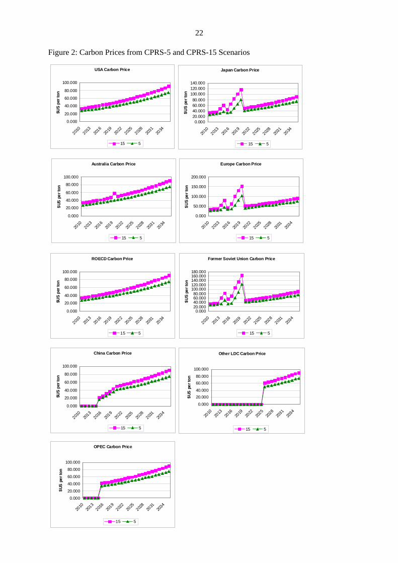
The results for carbon prices for the CPRS scenarios in the Green Paper are contained
in Figure 2. In this case a similar methodology is used except that countries enter the markets
at different times and there are some restrictions on trading. This shows up in the price
volatility especially for high marginal cost countries such as Japan, Europe and the Former
Soviet Union. Removal of trade restrictions enables more smoothing of the carbon price.
There is a slight spike in Australia in 2019 as constraints on trading are reached.
Several issues stand out in the results. The first is that the restrictions on permit trades
causes volatility in some variables for some countries. Spikes in carbon prices translate into
spikes in economic activity. This will vary in practice depending on a range of assumptions.
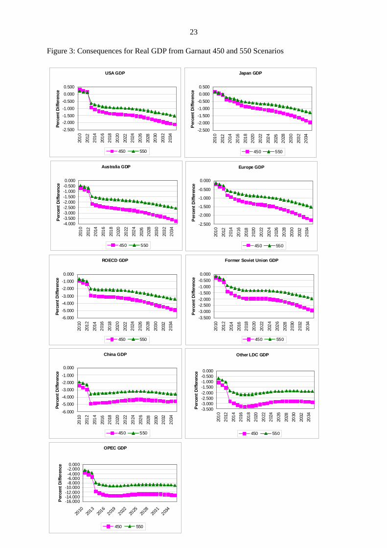
Secondly as countries face a binding emissions constraint, their GDP falls in the early years
of entry significantly. The short run dynamics and the long run averaging of costs over many
years are quite different in their implications than the short run adjustment. Under the
Garnaut-450 trajectory, Australia’s GDP is projected to fall by over 2 percent lower on
average than base over the first five years (see Figure 3). A large part of the economic costs
occur up front and then gradually rise over time as adjustments occur, and firms and
households have time to adjust to the new innovations induced by the carbon price. For
industrialized economies the GDP reduction in the first five years range from 0.25 percent for
15
Japan to 3 percent for the rest of the OECD in 2013 for the 450ppm scenario and two thirds
of that for the 550ppm scenario. Interestingly for the Garnaut scenarios developing countries
(who also enter in 2013) face similarly large GDP losses, in particular OPEC economies face
enormous losses in GDP in the initial years of 12 percent of GDP for the 450 scenario. Even
allowing income transfers through permit trading does not reduce the GDP losses, although it
does reduce the GNP losses since permit transfers are included in GNP. Despite these
transfers, GNP is still below base from 2013 in both Garnaut scenarios. It is clear that despite
the transfers through permit trading to developing countries there are still negative
implications of taking a domestic carbon price at the same time as the industrial economies.
Just transferring money for permits is not sufficient to give substantial differentiation in
economic costs. This point is not new and is familiar from a decade of literature (see for
example McKibbin, Shackleton and Wilcoxen (1999).
The results for GDP and GNP for the Green Paper CPRS scenarios are contained in
Figures 4 and 6. Recall that the carbon pricing policy begins earlier than the Garnaut
scenarios - in 2010 - and have a different phasing on the timing of each country’s entry. Costs
rise sharply in high abatement cost countries like Japan, Europe and Former Soviet Union
until 2020 due to limits on trading7.
Results for private investment for each scenario are shown in Figures 7 and 8. There
are two different forces acting on private investment in each economy. The announcement of
the policy in 2007 to begin either in 2010 or 2013 mean that some sectors that are carbon
intensive will anticipate the decline in the return on capital in their sector and cut back
investment. Other firms will ramp up investment in anticipation of the gains to new
technologies and investments in non carbon emitting inputs. This anticipation effect is
7 Spikes in prices that can be possible under the system modeled can be eliminated as argued by McKibbin and Wilcoxen
(2008) in a coordinated system of national pricing system.

16
important in the G-Cubed model because of the role of forward looking expectations in
decision making and because financial markets provide support in investing for expected
future gains. The other factor weighing on investment is the expected future slowdown of the
global economy as a result of the near term carbon constraint where the overall reduction in
economic activity reduces the expected return to capital. In some cases, countries that are
most affected will have a more negative impact of expected returns and financial capital will
flow from those economies to economies with less impacted expected returns. The flows of
capital will shown up as an improvement in the current accounts of countries losing capital
and a worsening in the current accounts of countries that are gaining foreign capital inflow.
In Figures 5 and 6 The United States and Japan experience initially stronger investment
where countries like Australia and other Annex B countries experience weaker investment.
Global capital flows to the larger economies away from fossil fuel intensive economies. This
effect was noted in McKibbin, Shackelton and Wilcoxen (1999). This makes the loss in GDP
larger for the countries losing capital and smaller for the countries gaining capital. Note that
the negative investment effects are larger for the developing economies.
The impact of the policies on the current account for each country is shown in Figures
10 and 11. As anticipated above, countries such as the United States experience a worsening
in their current account as capital flows in whereas Australia experiences an improvement in
the current account as capital flows out. Unfortunately all the developing regions experience
capital outflows due to the return to capital falling in these economies.
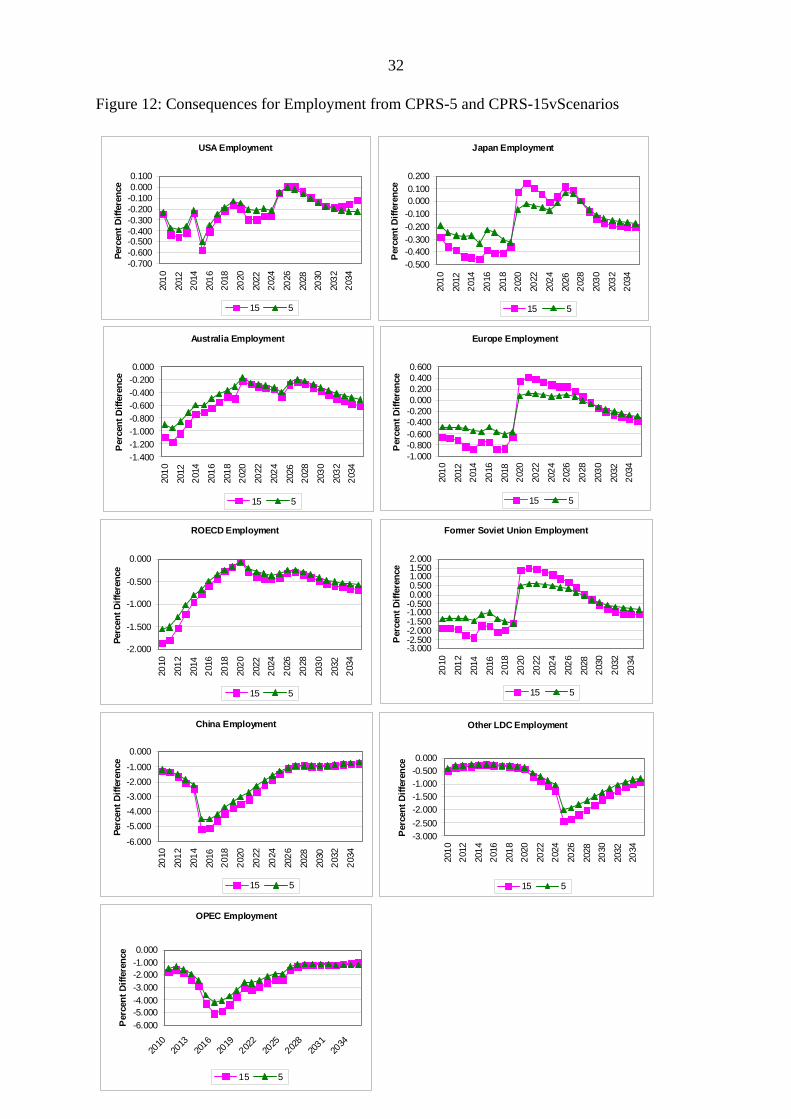
One of the strengths of the G-Cubed model is that it is not an equilibrium model in the
short run. Labour market rigidities, sticky prices and adjustment costs mean that it takes
many decades for equilibrium to be restored after an economic shock. This is shown clearly
in the results for employment shown in Figures 11 and 12. The results are deviations from a
reference scenario trajectory in which economies were moving from various degrees of
excess demand and excess supply of labour towards a long run steady state in which all

17
workers are eventually employed, subject to permanent structural rigidities. In all economies
the carbon constraint causes a fall in employment for the three decades shown in the graphs.
Eventually wages will adjust downwards relative to producer prices to ensure all workers are
eventually employed. The reason for the decline in employment at the national level is due to
the slowdown in overall economic activity globally, and the stickiness of real wages in which
the carbon price induced spike in consumer price leads to higher wage claims which reduce
the demand for labour. Individual sectors that are carbon intensive lose jobs that are not
quickly created by other expanding sectors because of the overall decline in economic
activity and spike in real wages. In Australia the average employment loss over the first five
years is 1 percent under the Garnaut 450 scenario and 0.5 percent under the Garnaut 550
scenario. The CPRS has a similar initial impact but after a decade employment returns close
to reference scenario.
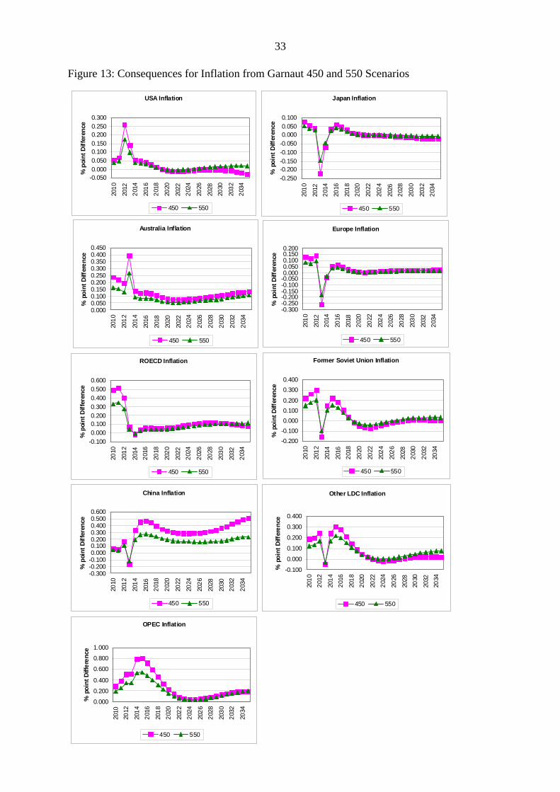
The results for inflation are shown in Figures 13 and 14. It is important to stress that
inflation is partly driven by the carbon constraint but also by the reaction of monetary
authorities in each economy in response to the changing economic conditions. The monetary
rule in each economy differs. The behavior of each region’s central bank follows a region-
specific Henderson-McKibbin-Taylor rule with a weight on output growth relative to trend, a
weight on inflation relative to trend and a weight on exchange rate volatility.8 The weights
vary across countries with industrialized economies focusing on controlling inflation and
output volatility, and developing countries placing a large weight on pegging the exchange
rate to the US dollar. Thus inflation is controlled eventually by all monetary authorities with
different short run responses depending on the relative weights on inflation versus output loss.
The introduction of the Garnaut 450 scenario causes Australian inflation to spike by 0.4% and
for the Garnaut-550 scenario to spike by 0.2% in the initial year of the policy. The CPRS
8 See Henderson and McKibbin (1993) and Taylor (1993).
18
scenarios have a slightly higher inflation spike of 0.7 percent and 0.5 percent for the 15
percent and 5 percent cuts. As with the other variables in the model, inflation tends to be
volatile around a small range once the various country entry assumptions are taken into
account.
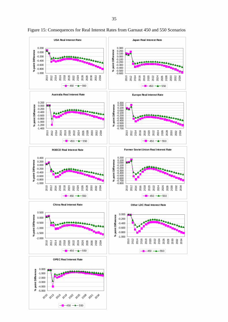
As mentioned above, the change in the carbon price reduces the return to capital in the
short run. Figures 15 and 16 show that this translates into a decline in real interest rates of
between 0.2 percentage points and 4 percentage points for the Garnaut 450 scenario. The
longer run change in real interest rates is directly related to the global changes in the return to
capital. The short run changes are a combination of this effect and the change in the short
term nominal interest rates set by the monetary authorities in each economy. The differences
across economies reflect the expected changes in real exchange rates over time. As a highly
greenhouse intensive economy, OPEC experiences a significant fall in real interest rates. This
is followed by Australia. In the case of the CPRS scenarios the adjustment path is more
volatile reflecting the volatility in other asset prices and economic activity. The overall trend
is similar to the Garnaut scenarios.
Figures 17 and 18 contain the results for the share market valuations. This is the total
value of all shares. Equity markets fall in all economies upon announcement of the policies
with an additional step down when the policies are implemented. The fall in share markets in
Australia is between 2 percent and 4 percent initially for the four scenarios. They then drift
lower over time reflecting the permanent decline in economic growth relative to reference
scenario. There is some volatility in prices in the CPRS scenarios as already outlined. The
relatively small fall in share markets reflect the anticipation of the largest impact being up
front but the long term changes in profitability is less affected
Finally results for the real effective exchange rates are shown in Figures 19 and 20.
The real effective exchange rate is defined in such a way that a rise is an appreciation. As
expected countries that are relatively fossil fuel intensive such as Australia and ROECD

19
experience a fall in their real exchange rate although there are a wide range of differences.
Partly this reflects the general equilibrium effects of the structure of production, aggregate
production outcomes, and the responses of monetary authorities. The outcomes are relatively
small because all countries are taking on carbon constraints. A single country taking action
would experience a much larger change in its real exchange rate.
6 Summary and Conclusions
This report has focused on the short run to medium run impacts of the four scenarios
for global emissions trading in a carbon constrained world. It is found that the very short run
impacts are significant in the model used although over time adjustment is relatively smooth.
These results are insightful not because of the specific sign of the outcomes but because they
show a number of important points. Firstly arbitrary restrictions on the global carbon market
and access to that market can generate volatility in carbon prices and asset prices generally. It
is not obvious that there are gains to this volatility and thus a strong case can be made to
build into policy a capacity to smooth this price volatility. Smoothing of the carbon price in
the short run will not necessarily occur because this volatility depends on what actually
occurs in future years across a wide range of economic realities. However the results for the
scenarios in this report show that excessive short term price volatility can occur in which case
it should be taken into account in the system design. Access to global carbon markets if
possible, can reduce this problem as might complete banking and borrowing of permits if
systems are well designed.
Secondly, developing countries have a significant impact on the price of carbon in
industrialized economies.
Thirdly, by linking developing countries into a global carbon price regime, these
countries incur adjustment costs which are not necessarily offset sufficiently by “fair” permit
allocations such as those under the contraction and convergence allocations modeled.

20
Finally it is important to understand the short run aggregate effects of policy shifts
such as an emission trading system that may deliver emissions reductions with a reasonable
economic outcome on average over half a century but which needs to survive the initial years
of dislocation and adjustment in order to be sustained. Due to technical problems this report
has not modeled the impact of transitional policy measures but the report does demonstrate
the importance of dealing with transitional issues in whatever policy framework is designed,
independently of how good the policy may look in the longer run.

21
Figure 1: Carbon Prices from Garnaut 450 and 550 Scenario
USA carbon price
0.000
20.000
40.000
60.000
80.000
100.000
2010
2013
2016
2019
2022
2025
2028
2031
2034
$US
per t
on
450 550
Japan carbon price
0.000
20.000
40.000
60.000
80.000
100.000
2010
2013
2016
2019
2022
2025
2028
2031
2034
$US
per t
on
450 550
Australia carbon price
0.000
20.000
40.000
60.000
80.000
100.000
2010
2013
2016
2019
2022
2025
2028
2031
2034
$US
per
ton
450 550
Europe carbon price
0.000
20.000
40.000
60.000
80.000
100.000
2010
2013
2016
2019
2022
2025
2028
2031
2034
$US
per t
on
450 550
ROECD carbon price
0.000
20.000
40.000
60.000
80.000
100.000
2010
2013
2016
2019
2022
2025
2028
2031
2034
$US
per t
on
450 550
Former Soviet Union carbon price
0.000
20.000
40.000
60.000
80.000
100.000
2010
2013
2016
2019
2022
2025
2028
2031
2034
$US
per t
on
450 550
China carbon price
0.000
20.000
40.000
60.000
80.000
100.000
2010
2013
2016
2019
2022
2025
2028
2031
2034
$US
per t
on
450 550
Other LDC carbon price
0.00020.000
40.00060.000
80.000100.000
2010
2013
2016
2019
2022
2025
2028
2031
2034
$US
per
ton
450 550
OPEC carbon price
0.00020.00040.00060.00080.000
100.000
2010
2013
2016
2019
2022
2025
2028
2031
2034
$US
per
ton
450 550
22
Figure 2: Carbon Prices from CPRS-5 and CPRS-15 Scenarios
USA Carbon Price
0.000
20.000
40.000
60.000
80.000
100.000
2010
2013
2016
2019
2022
2025
2028
2031
2034
$US
per t
on
15 5
Japan Carbon Price
0.00020.00040.00060.00080.000
100.000120.000140.000
2010
2013
2016
2019
2022
2025
2028
2031
2034
$US
per t
on
15 5
Australia Carbon Price
0.000
20.000
40.000
60.000
80.000
100.000
2010
2013
2016
2019
2022
2025
2028
2031
2034
$US
per
ton
15 5
Europe Carbon Price
0.000
50.000
100.000
150.000
200.000
2010
2013
2016
2019
2022
2025
2028
2031
2034
$US
per t
on
15 5
ROECD Carbon Price
0.000
20.000
40.000
60.000
80.000
100.000
2010
2013
2016
2019
2022
2025
2028
2031
2034
$US
per t
on
15 5
Former Soviet Union Carbon Price
0.00020.00040.00060.00080.000
100.000120.000140.000160.000180.000
2010
2013
2016
2019
2022
2025
2028
2031
2034
$US
per t
on
15 5
China Carbon Price
0.000
20.000
40.000
60.000
80.000
100.000
2010
2013
2016
2019
2022
2025
2028
2031
2034
$US
per t
on
15 5
Other LDC Carbon Price
0.000
20.00040.000
60.00080.000
100.000
2010
2013
2016
2019
2022
2025
2028
2031
2034
$US
per
ton
15 5
OPEC Carbon Price
0.000
20.000
40.000
60.000
80.000
100.000
2010
2013
2016
2019
2022
2025
2028
2031
2034
$US
per
ton
15 5
23
Figure 3: Consequences for Real GDP from Garnaut 450 and 550 Scenarios
USA GDP
-2.500-2.000-1.500-1.000-0.5000.0000.500
2010
2012
2014
2016
2018
2020
2022
2024
2026
2028
2030
2032
2034
Perc
ent D
iffer
ence
450 550
Japan GDP
-2.500-2.000-1.500-1.000-0.5000.0000.500
2010
2012
2014
2016
2018
2020
2022
2024
2026
2028
2030
2032
2034
Per
cent
Diff
eren
ce
450 550
Australia GDP
-4.000-3.500-3.000-2.500-2.000-1.500-1.000-0.5000.000
2010
2012
2014
2016
2018
2020
2022
2024
2026
2028
2030
2032
2034
Per
cent
Diff
eren
ce
450 550
Europe GDP
-2.500
-2.000
-1.500
-1.000
-0.500
0.000
2010
2012
2014
2016
2018
2020
2022
2024
2026
2028
2030
2032
2034
Per
cent
Diff
eren
ce
450 550
ROECD GDP
-6.000-5.000-4.000-3.000
-2.000-1.0000.000
2010
2012
2014
2016
2018
2020
2022
2024
2026
2028
2030
2032
2034
Perc
ent D
iffer
ence
450 550
Former Soviet Union GDP
-3.500-3.000-2.500-2.000-1.500-1.000-0.5000.000
2010
2012
2014
2016
2018
2020
2022
2024
2026
2028
2030
2032
2034
Per
cent
Diff
eren
ce
450 550
China GDP
-6.000
-5.000-4.000-3.000-2.000-1.000
0.000
2010
2012
2014
2016
2018
2020
2022
2024
2026
2028
2030
2032
2034
Perc
ent D
iffer
ence
450 550
Other LDC GDP
-3.500-3.000-2.500-2.000-1.500-1.000-0.5000.000
2010
2012
2014
2016
2018
2020
2022
2024
2026
2028
2030
2032
2034
Per
cent
Diff
eren
ce
450 550
OPEC GDP
-16.000-14.000-12.000-10.000-8.000-6.000-4.000-2.0000.000
2010
2013
2016
2019
2022
2025
2028
2031
2034
Per
cent
Diff
eren
ce
450 550

24
Figure 4: Consequences for Real GDP from CPRS-5 and CPRS-15 Scenarios
USA GDP
-2.000
-1.500
-1.000
-0.500
0.00020
10
2012
2014
2016
2018
2020
2022
2024
2026
2028
2030
2032
2034
Perc
ent D
iffer
ence
15 5
Japan GDP
-2.500
-2.000
-1.500
-1.000
-0.500
0.000
2010
2012
2014
2016
2018
2020
2022
2024
2026
2028
2030
2032
2034
Per
cent
Diff
eren
ce
15 5
Australia GDP
-5.000
-4.000
-3.000
-2.000
-1.000
0.000
2010
2012
2014
2016
2018
2020
2022
2024
2026
2028
2030
2032
2034
Per
cent
Diff
eren
ce
15 5
Europe GDP
-3.500-3.000-2.500-2.000-1.500-1.000-0.5000.000
2010
2012
2014
2016
2018
2020
2022
2024
2026
2028
2030
2032
2034
Per
cent
Diff
eren
ce
15 5
ROECD GDP
-6.000-5.000-4.000-3.000-2.000-1.0000.000
2010
2012
2014
2016
2018
2020
2022
2024
2026
2028
2030
2032
2034
Perc
ent D
iffer
ence
15 5
Former Soviet Union GDP
-5.000
-4.000
-3.000
-2.000
-1.000
0.000
2010
2012
2014
2016
2018
2020
2022
2024
2026
2028
2030
2032
2034
Per
cent
Diff
eren
ce
15 5
China GDP
-6.000
-5.000-4.000-3.000-2.000-1.000
0.000
2010
2012
2014
2016
2018
2020
2022
2024
2026
2028
2030
2032
2034
Perc
ent D
iffer
ence
15 5
Other LDC GDP
-4.000
-3.000
-2.000
-1.000
0.000
2010
2012
2014
2016
2018
2020
2022
2024
2026
2028
2030
2032
2034
Per
cent
Diff
eren
ce
15 5
OPEC GDP
-14.000-12.000-10.000-8.000-6.000-4.000-2.0000.000
2010
2013
2016
2019
2022
2025
2028
2031
2034
Per
cent
Diff
eren
ce
15 5

25
Figure 5: Consequences for Real GNP from Garnaut 450 and 550 Scenarios
USA GNP
-2.500-2.000-1.500-1.000-0.5000.0000.500
2010
2012
2014
2016
2018
2020
2022
2024
2026
2028
2030
2032
2034
Perc
ent D
iffer
ence
450 550
Japan GNP
-4.000
-3.000
-2.000
-1.000
0.000
1.000
2010
2012
2014
2016
2018
2020
2022
2024
2026
2028
2030
2032
2034
Per
cent
Diff
eren
ce
450 550
Australia GNP
-4.000-3.500-3.000-2.500-2.000-1.500-1.000-0.5000.000
2010
2012
2014
2016
2018
2020
2022
2024
2026
2028
2030
2032
2034
Per
cent
Diff
eren
ce
450 550
Europe GNP
-3.500-3.000-2.500-2.000-1.500-1.000-0.5000.000
2010
2012
2014
2016
2018
2020
2022
2024
2026
2028
2030
2032
2034
Per
cent
Diff
eren
ce
450 550
ROECD GNP
-5.000
-4.000
-3.000
-2.000
-1.000
0.000
2010
2012
2014
2016
2018
2020
2022
2024
2026
2028
2030
2032
2034
Perc
ent D
iffer
ence
450 550
Former Soviet Union GNP
-4.000-3.500-3.000-2.500-2.000-1.500-1.000-0.5000.000
2010
2012
2014
2016
2018
2020
2022
2024
2026
2028
2030
2032
2034
Per
cent
Diff
eren
ce
450 550
China GNP
-3.500-3.000-2.500-2.000-1.500-1.000-0.5000.000
2010
2012
2014
2016
2018
2020
2022
2024
2026
2028
2030
2032
2034
Perc
ent D
iffer
ence
450 550
Other LDC GNP
-3.500-3.000-2.500-2.000-1.500-1.000-0.5000.000
2010
2012
2014
2016
2018
2020
2022
2024
2026
2028
2030
2032
2034
Per
cent
Diff
eren
ce
450 550
OPEC GNP
-14.000-12.000-10.000-8.000-6.000-4.000-2.0000.000
2010
2013
2016
2019
2022
2025
2028
2031
2034
Per
cent
Diff
eren
ce
450 550

26
Figure 6: Consequences for Real GNP from CPRS-5 and CPRS-15 Scenarios
USA GNP
-2.500
-2.000
-1.500
-1.000
-0.500
0.00020
10
2012
2014
2016
2018
2020
2022
2024
2026
2028
2030
2032
2034
Perc
ent D
iffer
ence
15 5
Japan GNP
-3.500-3.000-2.500-2.000-1.500-1.000-0.5000.000
2010
2012
2014
2016
2018
2020
2022
2024
2026
2028
2030
2032
2034
Per
cent
Diff
eren
ce
15 5
Australia GNP
-4.000-3.500-3.000-2.500-2.000-1.500-1.000-0.5000.000
2010
2012
2014
2016
2018
2020
2022
2024
2026
2028
2030
2032
2034
Per
cent
Diff
eren
ce
15 5
Europe GNP
-3.500-3.000-2.500-2.000-1.500-1.000-0.5000.000
2010
2012
2014
2016
2018
2020
2022
2024
2026
2028
2030
2032
2034
Per
cent
Diff
eren
ce
15 5
ROECD GNP
-4.500-4.000-3.500-3.000-2.500-2.000-1.500-1.000-0.5000.000
2010
2012
2014
2016
2018
2020
2022
2024
2026
2028
2030
2032
2034
Perc
ent D
iffer
ence
15 5
Former Soviet Union GNP
-4.500-4.000-3.500-3.000-2.500-2.000-1.500-1.000-0.5000.000
2010
2012
2014
2016
2018
2020
2022
2024
2026
2028
2030
2032
2034
Per
cent
Diff
eren
ce
15 5
China GNP
-6.000
-5.000-4.000-3.000-2.000-1.000
0.000
2010
2012
2014
2016
2018
2020
2022
2024
2026
2028
2030
2032
2034
Perc
ent D
iffer
ence
15 5
Other LDC GNP
-4.000
-3.000
-2.000
-1.000
0.000
2010
2012
2014
2016
2018
2020
2022
2024
2026
2028
2030
2032
2034
Per
cent
Diff
eren
ce
15 5
OPEC GNP
-14.000-12.000-10.000-8.000-6.000-4.000-2.0000.000
2010
2013
2016
2019
2022
2025
2028
2031
2034
Per
cent
Diff
eren
ce
15 5

27
Figure 7: Consequences for Private Investment from Garnaut 450 and 550 Scenarios
USA Investment
-3.000
-2.000
-1.000
0.000
1.000
2.00020
10
2012
2014
2016
2018
2020
2022
2024
2026
2028
2030
2032
2034
Perc
ent D
iffer
ence
450 550
Japan Investment
-3.000-2.000-1.0000.0001.0002.0003.000
2010
2012
2014
2016
2018
2020
2022
2024
2026
2028
2030
2032
2034
Per
cent
Diff
eren
ce
450 550
Australia Investment
-7.000-6.000-5.000-4.000-3.000-2.000-1.0000.000
2010
2012
2014
2016
2018
2020
2022
2024
2026
2028
2030
2032
2034
Per
cent
Diff
eren
ce
450 550
Europe Investment
-6.000-5.000-4.000-3.000-2.000-1.0000.000
2010
2012
2014
2016
2018
2020
2022
2024
2026
2028
2030
2032
2034
Per
cent
Diff
eren
ce
450 550
ROECD Investment
-14.000-12.000-10.000-8.000-6.000-4.000-2.0000.000
2010
2013
2016
2019
2022
2025
2028
2031
2034
Perc
ent D
iffer
ence
450 550
Former Soviet Union Investment
-8.000-7.000-6.000-5.000-4.000-3.000-2.000-1.0000.000
2010
2012
2014
2016
2018
2020
2022
2024
2026
2028
2030
2032
2034
Per
cent
Diff
eren
ce
450 550
China Investment
-10.000
-8.000
-6.000
-4.000
-2.000
0.000
2010
2012
2014
2016
2018
2020
2022
2024
2026
2028
2030
2032
2034
Perc
ent D
iffer
ence
450 550
Other LDC Investment
-7.000-6.000-5.000-4.000-3.000-2.000-1.0000.000
2010
2012
2014
2016
2018
2020
2022
2024
2026
2028
2030
2032
2034
Per
cent
Diff
eren
ce
450 550
OPEC Investment
-30.000-25.000-20.000-15.000-10.000-5.0000.000
2010
2013
2016
2019
2022
2025
2028
2031
2034
Per
cent
Diff
eren
ce
450 550

28
Figure 8: Consequences for Private Investment from CPRS-5 and CPRS-15 Scenarios
USA Investment
-2.000-1.500-1.000-0.5000.0000.5001.000
2010
2012
2014
2016
2018
2020
2022
2024
2026
2028
2030
2032
2034
Perc
ent D
iffer
ence
15 5
Japan Investment
-12.000-10.000-8.000-6.000-4.000-2.0000.0002.0004.000
2010
2013
2016
2019
2022
2025
2028
2031
2034
Per
cent
Diff
eren
ce
15 5
Australia Investment
-8.000-7.000-6.000-5.000-4.000-3.000-2.000-1.0000.000
2010
2012
2014
2016
2018
2020
2022
2024
2026
2028
2030
2032
2034
Per
cent
Diff
eren
ce
15 5
Europe Investment
-7.000-6.000-5.000-4.000-3.000-2.000-1.0000.000
2010
2012
2014
2016
2018
2020
2022
2024
2026
2028
2030
2032
2034
Per
cent
Diff
eren
ce
15 5
ROECD Investment
-16.000-14.000-12.000-10.000-8.000-6.000-4.000-2.0000.000
2010
2013
2016
2019
2022
2025
2028
2031
2034
Perc
ent D
iffer
ence
15 5
Former Soviet Union Investment
-12.000-10.000-8.000
-6.000-4.000-2.000
0.000
2010
2012
2014
2016
2018
2020
2022
2024
2026
2028
2030
2032
2034
Per
cent
Diff
eren
ce
15 5
China Investment
-10.000
-8.000
-6.000
-4.000
-2.000
0.000
2010
2012
2014
2016
2018
2020
2022
2024
2026
2028
2030
2032
2034
Perc
ent D
iffer
ence
15 5
Other LDC Investment
-7.000-6.000-5.000-4.000-3.000-2.000-1.0000.000
2010
2012
2014
2016
2018
2020
2022
2024
2026
2028
2030
2032
2034
Per
cent
Diff
eren
ce
15 5
OPEC Investment
-25.000-20.000
-15.000-10.000
-5.0000.000
2010
2013
2016
2019
2022
2025
2028
2031
2034
Per
cent
Diff
eren
ce
15 5

29
Figure 9: Consequences for Current Account from Garnaut 450 and 550 Scenarios
USA Current Account
-0.600-0.500-0.400-0.300-0.200-0.1000.000
2010
2012
2014
2016
2018
2020
2022
2024
2026
2028
2030
2032
2034
Perc
ent G
DP D
iffer
ence
450 550
Japan Current Account
-3.500-3.000-2.500-2.000-1.500-1.000-0.5000.000
2010
2012
2014
2016
2018
2020
2022
2024
2026
2028
2030
2032
2034
Per
cent
GD
P D
iffer
ence
450 550
Australia Current Account
0.000
0.200
0.400
0.600
0.800
1.000
2010
2012
2014
2016
2018
2020
2022
2024
2026
2028
2030
2032
2034
Per
cent
GD
P D
iffer
ence
450 550
Europe Current Account
-1.200-1.000-0.800-0.600-0.400-0.2000.000
2010
2012
2014
2016
2018
2020
2022
2024
2026
2028
2030
2032
2034
Per
cent
GD
P D
iffer
ence
450 550
ROECD Current Account
0.0000.2000.4000.6000.8001.0001.2001.400
2010
2012
2014
2016
2018
2020
2022
2024
2026
2028
2030
2032
2034
Perc
ent G
DP D
iffer
ence
450 550
Former Soviet Union Current Account
-0.200
-0.150
-0.100
-0.050
0.000
0.050
2010
2012
2014
2016
2018
2020
2022
2024
2026
2028
2030
2032
2034
Per
cent
GD
P D
iffer
ence
450 550
China Current Account
0.0000.5001.0001.5002.0002.5003.0003.5004.0004.500
2010
2012
2014
2016
2018
2020
2022
2024
2026
2028
2030
2032
2034
Perc
ent G
DP D
iffer
ence
450 550
Other LDC Current Account
0.000
0.200
0.400
0.600
0.800
2010
2012
2014
2016
2018
2020
2022
2024
2026
2028
2030
2032
2034P
erce
nt G
DP
Diff
eren
ce
450 550
OPEC Current Account
0.0000.5001.0001.5002.0002.5003.0003.5004.000
2010
2012
2014
2016
2018
2020
2022
2024
2026
2028
2030
2032
2034P
erce
nt G
DP D
iffer
ence
450 550

30
Figure 10: Consequences for Current Account from CPRS-5 and CPRS-15vScenarios
USA Current Account
-1.200-1.000-0.800-0.600-0.400-0.2000.000
2010
2012
2014
2016
2018
2020
2022
2024
2026
2028
2030
2032
2034
Perc
ent G
DP D
iffer
ence
15 5
Japan Current Account
-3.000-2.500-2.000-1.500-1.000-0.5000.000
2010
2012
2014
2016
2018
2020
2022
2024
2026
2028
2030
2032
2034
Per
cent
GD
P D
iffer
ence
15 5
Australia Current Account
0.0000.2000.4000.6000.8001.0001.2001.4001.600
2010
2012
2014
2016
2018
2020
2022
2024
2026
2028
2030
2032
2034
Per
cent
GD
P D
iffer
ence
15 5
Europe Current Account
-1.000-0.800-0.600-0.400
-0.2000.0000.200
2010
2012
2014
2016
2018
2020
2022
2024
2026
2028
2030
2032
2034
Per
cent
GD
P D
iffer
ence
15 5
ROECD Current Account
0.000
0.500
1.000
1.500
2.000
2.500
2010
2012
2014
2016
2018
2020
2022
2024
2026
2028
2030
2032
2034
Perc
ent G
DP D
iffer
ence
15 5
Former Soviet Union Current Account
0.0000.2000.4000.6000.8001.0001.2001.4001.600
2010
2012
2014
2016
2018
2020
2022
2024
2026
2028
2030
2032
2034
Per
cent
GD
P D
iffer
ence
15 5
China Current Account
0.000
0.500
1.000
1.500
2.000
2.500
2010
2012
2014
2016
2018
2020
2022
2024
2026
2028
2030
2032
2034
Perc
ent G
DP D
iffer
ence
15 5
Other LDC Current Account
0.0000.2000.4000.6000.8001.0001.200
2010
2012
2014
2016
2018
2020
2022
2024
2026
2028
2030
2032
2034P
erce
nt G
DP
Diff
eren
ce
15 5
OPEC Current Account
-2.000-1.500-1.000-0.5000.0000.5001.0001.5002.000
2010
2013
2016
2019
2022
2025
2028
2031
2034
Per
cent
GD
P D
iffer
ence
15 5

31
Figure 11: Consequences for Employment from Garnaut 450 and 550 Scenarios
USA Employment
-1.000-0.800-0.600-0.400-0.2000.0000.200
2010
2012
2014
2016
2018
2020
2022
2024
2026
2028
2030
2032
2034
Perc
ent D
iffer
ence
450 550
Japan Employment
-0.500-0.400-0.300-0.200-0.1000.0000.100
2010
2012
2014
2016
2018
2020
2022
2024
2026
2028
2030
2032
2034
Per
cent
Diff
eren
ce
450 550
Australia Employment
-1.400-1.200-1.000-0.800-0.600-0.400-0.2000.000
2010
2012
2014
2016
2018
2020
2022
2024
2026
2028
2030
2032
2034
Per
cent
Diff
eren
ce
450 550
Europe Employment
-0.800-0.700-0.600-0.500-0.400-0.300-0.200-0.1000.000
2010
2012
2014
2016
2018
2020
2022
2024
2026
2028
2030
2032
2034
Per
cent
Diff
eren
ce
450 550
ROECD Employment
-2.000
-1.500
-1.000
-0.500
0.000
2010
2012
2014
2016
2018
2020
2022
2024
2026
2028
2030
2032
2034
Perc
ent D
iffer
ence
450 550
Former Soviet Union Employment
-1.600-1.400-1.200-1.000-0.800-0.600-0.400-0.2000.000
2010
2012
2014
2016
2018
2020
2022
2024
2026
2028
2030
2032
2034
Per
cent
Diff
eren
ce
450 550
China Employment
-5.000
-4.000
-3.000
-2.000
-1.000
0.000
2010
2012
2014
2016
2018
2020
2022
2024
2026
2028
2030
2032
2034
Perc
ent D
iffer
ence
450 550
Other LDC Employment
-2.000
-1.500
-1.000
-0.500
0.000
2010
2012
2014
2016
2018
2020
2022
2024
2026
2028
2030
2032
2034
Per
cent
Diff
eren
ce
450 550
OPEC Employment
-6.000-5.000-4.000-3.000-2.000-1.0000.000
2010
2013
2016
2019
2022
2025
2028
2031
2034
Per
cent
Diff
eren
ce
450 550
32
Figure 12: Consequences for Employment from CPRS-5 and CPRS-15vScenarios
USA Employment
-0.700-0.600-0.500-0.400-0.300-0.200-0.1000.0000.100
2010
2012
2014
2016
2018
2020
2022
2024
2026
2028
2030
2032
2034
Perc
ent D
iffer
ence
15 5
Japan Employment
-0.500-0.400-0.300-0.200-0.1000.0000.1000.200
2010
2012
2014
2016
2018
2020
2022
2024
2026
2028
2030
2032
2034
Per
cent
Diff
eren
ce
15 5
Australia Employment
-1.400-1.200-1.000-0.800-0.600-0.400-0.2000.000
2010
2012
2014
2016
2018
2020
2022
2024
2026
2028
2030
2032
2034
Per
cent
Diff
eren
ce
15 5
Europe Employment
-1.000-0.800-0.600-0.400-0.2000.0000.2000.4000.600
2010
2012
2014
2016
2018
2020
2022
2024
2026
2028
2030
2032
2034
Per
cent
Diff
eren
ce
15 5
ROECD Employment
-2.000
-1.500
-1.000
-0.500
0.000
2010
2012
2014
2016
2018
2020
2022
2024
2026
2028
2030
2032
2034
Perc
ent D
iffer
ence
15 5
Former Soviet Union Employment
-3.000-2.500-2.000-1.500-1.000-0.5000.0000.5001.0001.5002.000
2010
2012
2014
2016
2018
2020
2022
2024
2026
2028
2030
2032
2034
Per
cent
Diff
eren
ce
15 5
China Employment
-6.000
-5.000-4.000-3.000-2.000-1.000
0.000
2010
2012
2014
2016
2018
2020
2022
2024
2026
2028
2030
2032
2034
Perc
ent D
iffer
ence
15 5
Other LDC Employment
-3.000-2.500-2.000-1.500-1.000-0.5000.000
2010
2012
2014
2016
2018
2020
2022
2024
2026
2028
2030
2032
2034
Perc
ent D
iffer
ence
15 5
OPEC Employment
-6.000-5.000-4.000-3.000-2.000-1.0000.000
2010
2013
2016
2019
2022
2025
2028
2031
2034
Per
cent
Diff
eren
ce
15 5
33
Figure 13: Consequences for Inflation from Garnaut 450 and 550 Scenarios
USA Inflation
-0.0500.0000.0500.1000.1500.2000.2500.300
2010
2012
2014
2016
2018
2020
2022
2024
2026
2028
2030
2032
2034
% p
oint
Diff
eren
ce
450 550
Japan Inflation
-0.250-0.200-0.150-0.100-0.0500.0000.0500.100
2010
2012
2014
2016
2018
2020
2022
2024
2026
2028
2030
2032
2034
% p
oint
Diff
eren
ce
450 550
Australia Inflation
0.0000.0500.1000.1500.2000.2500.3000.3500.4000.450
2010
2012
2014
2016
2018
2020
2022
2024
2026
2028
2030
2032
2034
% p
oint
Diff
eren
ce
450 550
Europe Inflation
-0.300-0.250-0.200-0.150-0.100-0.0500.0000.0500.1000.1500.200
2010
2012
2014
2016
2018
2020
2022
2024
2026
2028
2030
2032
2034
% p
oint
Diff
eren
ce
450 550
ROECD Inflation
-0.1000.0000.1000.2000.3000.4000.5000.600
2010
2012
2014
2016
2018
2020
2022
2024
2026
2028
2030
2032
2034
% p
oint
Diff
eren
ce
450 550
Former Soviet Union Inflation
-0.200-0.1000.0000.1000.200
0.3000.400
2010
2012
2014
2016
2018
2020
2022
2024
2026
2028
2030
2032
2034
% p
oint
Diff
eren
ce
450 550
China Inflation
-0.300-0.200-0.1000.0000.1000.2000.3000.4000.5000.600
2010
2012
2014
2016
2018
2020
2022
2024
2026
2028
2030
2032
2034
% p
oint
Diff
eren
ce
450 550
Other LDC Inflation
-0.100
0.000
0.100
0.200
0.300
0.400
2010
2012
2014
2016
2018
2020
2022
2024
2026
2028
2030
2032
2034
% p
oint
Diff
eren
ce
450 550
OPEC Inflation
0.000
0.200
0.400
0.600
0.800
1.000
2010
2012
2014
2016
2018
2020
2022
2024
2026
2028
2030
2032
2034
% p
oint
Diff
eren
ce
450 550

34
Figure 14: Consequences for Inflation from CPRS-5 and CPRS-15vScenarios
USA Inflation
-0.400-0.2000.000
0.2000.400
0.60020
10
2012
2014
2016
2018
2020
2022
2024
2026
2028
2030
2032
2034
% p
oint
Diff
eren
ce
15 5
Japan Inflation
-0.300-0.200-0.1000.0000.1000.2000.300
2010
2012
2014
2016
2018
2020
2022
2024
2026
2028
2030
2032
2034
% p
oint
Diff
eren
ce
15 5
Australia Inflation
-0.600-0.400-0.2000.0000.2000.4000.6000.800
2010
2012
2014
2016
2018
2020
2022
2024
2026
2028
2030
2032
2034
% p
oint
Diff
eren
ce
15 5
Europe Inflation
-0.300
-0.200-0.1000.000
0.1000.2000.300
2010
2012
2014
2016
2018
2020
2022
2024
2026
2028
2030
2032
2034
% p
oint
Diff
eren
ce
15 5
ROECD Inflation
-0.200-0.1000.0000.1000.2000.3000.4000.5000.600
2010
2012
2014
2016
2018
2020
2022
2024
2026
2028
2030
2032
2034
% p
oint
Diff
eren
ce
15 5
Former Soviet Union Inflation
-0.600-0.400-0.2000.0000.2000.4000.600
2010
2012
2014
2016
2018
2020
2022
2024
2026
2028
2030
2032
2034
% p
oint
Diff
eren
ce
15 5
China Inflation
-0.400-0.2000.0000.2000.4000.6000.8001.000
2010
2012
2014
2016
2018
2020
2022
2024
2026
2028
2030
2032
2034
% p
oint
Diff
eren
ce
15 5
Other LDC Inflation
-0.400
-0.200
0.000
0.200
0.4000.600
2010
2012
2014
2016
2018
2020
2022
2024
2026
2028
2030
2032
2034
% p
oint
Diff
eren
ce
15 5
OPEC Inflation
-2.000-1.0000.0001.0002.0003.0004.000
2010
2013
2016
2019
2022
2025
2028
2031
2034
% p
oint
Diff
eren
ce
15 5
35
Figure 15: Consequences for Real Interest Rates from Garnaut 450 and 550 Scenarios
USA Real Interest Rate
-1.000-0.800-0.600-0.400-0.2000.0000.200
2010
2012
2014
2016
2018
2020
2022
2024
2026
2028
2030
2032
2034
% p
oint
Diff
eren
ce
450 550
Japan Real Interest Rate
-0.600-0.500-0.400-0.300-0.200-0.1000.0000.1000.2000.300
2010
2012
2014
2016
2018
2020
2022
2024
2026
2028
2030
2032
2034
% p
oint
Diff
eren
ce
450 550
Australia Real Interest Rate
-1.400-1.200-1.000-0.800-0.600-0.400-0.2000.0000.200
2010
2012
2014
2016
2018
2020
2022
2024
2026
2028
2030
2032
2034
% p
oint
Diff
eren
ce
450 550
Europe Real Interest Rate
-0.700-0.600-0.500-0.400-0.300-0.200-0.1000.0000.1000.2000.300
2010
2012
2014
2016
2018
2020
2022
2024
2026
2028
2030
2032
2034
% p
oint
Diff
eren
ce
450 550
ROECD Real Interest Rate
-1.000-0.800-0.600-0.400-0.2000.0000.2000.400
2010
2012
2014
2016
2018
2020
2022
2024
2026
2028
2030
2032
2034
% p
oint
Diff
eren
ce
450 550
Former Soviet Union Real Interest Rate
-0.800-0.700-0.600-0.500-0.400-0.300-0.200-0.1000.0000.1000.200
2010
2012
2014
2016
2018
2020
2022
2024
2026
2028
2030
2032
2034
% p
oint
Diff
eren
ce
450 550
China Real Interest Rate
-2.000
-1.500
-1.000
-0.500
0.000
0.500
2010
2012
2014
2016
2018
2020
2022
2024
2026
2028
2030
2032
2034
% p
oint
Diff
eren
ce
450 550
Other LDC Real Interest Rate
-1.000
-0.800
-0.600
-0.400
-0.200
0.000
2010
2012
2014
2016
2018
2020
2022
2024
2026
2028
2030
2032
2034
% p
oint
Diff
eren
ce
450 550
OPEC Real Interest Rate
-5.000-4.000
-3.000-2.000
-1.0000.000
2010
2013
2016
2019
2022
2025
2028
2031
2034
% p
oint
Diff
eren
ce
450 550
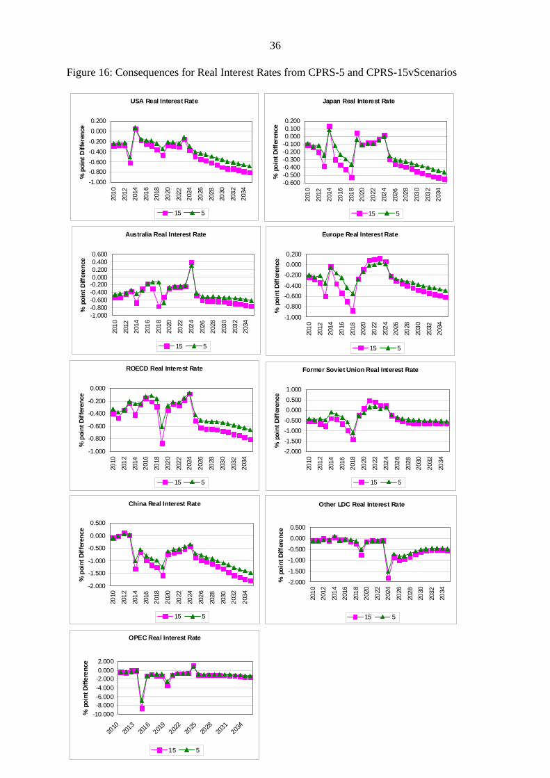
36
Figure 16: Consequences for Real Interest Rates from CPRS-5 and CPRS-15vScenarios
USA Real Interest Rate
-1.000-0.800-0.600-0.400-0.2000.0000.200
2010
2012
2014
2016
2018
2020
2022
2024
2026
2028
2030
2032
2034
% p
oint
Diff
eren
ce
15 5
Japan Real Interest Rate
-0.600-0.500-0.400-0.300-0.200-0.1000.0000.1000.200
2010
2012
2014
2016
2018
2020
2022
2024
2026
2028
2030
2032
2034
% p
oint
Diff
eren
ce
15 5
Australia Real Interest Rate
-1.000-0.800-0.600-0.400-0.2000.0000.2000.4000.600
2010
2012
2014
2016
2018
2020
2022
2024
2026
2028
2030
2032
2034
% p
oint
Diff
eren
ce
15 5
Europe Real Interest Rate
-1.000
-0.800-0.600-0.400
-0.2000.0000.200
2010
2012
2014
2016
2018
2020
2022
2024
2026
2028
2030
2032
2034
% p
oint
Diff
eren
ce
15 5
ROECD Real Interest Rate
-1.000
-0.800
-0.600
-0.400
-0.200
0.000
2010
2012
2014
2016
2018
2020
2022
2024
2026
2028
2030
2032
2034
% p
oint
Diff
eren
ce
15 5
Former Soviet Union Real Interest Rate
-2.000-1.500-1.000-0.5000.0000.5001.000
2010
2012
2014
2016
2018
2020
2022
2024
2026
2028
2030
2032
2034
% p
oint
Diff
eren
ce
15 5
China Real Interest Rate
-2.000
-1.500
-1.000
-0.500
0.000
0.500
2010
2012
2014
2016
2018
2020
2022
2024
2026
2028
2030
2032
2034
% p
oint
Diff
eren
ce
15 5
Other LDC Real Interest Rate
-2.000
-1.500
-1.000
-0.500
0.000
0.500
2010
2012
2014
2016
2018
2020
2022
2024
2026
2028
2030
2032
2034
% p
oint
Diff
eren
ce
15 5
OPEC Real Interest Rate
-10.000-8.000-6.000-4.000-2.0000.0002.000
2010
2013
2016
2019
2022
2025
2028
2031
2034
% p
oint
Diff
eren
ce
15 5
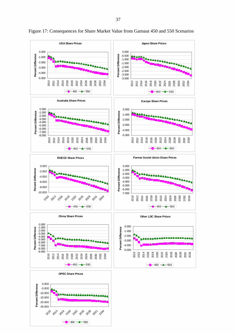
37
Figure 17: Consequences for Share Market Value from Garnaut 450 and 550 Scenarios
USA Share Prices
-5.000
-4.000
-3.000
-2.000
-1.000
0.00020
10
2012
2014
2016
2018
2020
2022
2024
2026
2028
2030
2032
2034
Perc
ent D
iffer
ence
450 550
Japan Share Prices
-3.500-3.000-2.500-2.000-1.500-1.000-0.5000.000
2010
2012
2014
2016
2018
2020
2022
2024
2026
2028
2030
2032
2034
Per
cent
Diff
eren
ce
450 550
Australia Share Prices
-8.000-7.000-6.000-5.000-4.000-3.000-2.000-1.0000.000
2010
2012
2014
2016
2018
2020
2022
2024
2026
2028
2030
2032
2034
Per
cent
Diff
eren
ce
450 550
Europe Share Prices
-5.000
-4.000
-3.000
-2.000
-1.000
0.000
2010
2012
2014
2016
2018
2020
2022
2024
2026
2028
2030
2032
2034
Per
cent
Diff
eren
ce
450 550
ROECD Share Prices
-10.000
-8.000
-6.000
-4.000
-2.000
0.000
2010
2013
2016
2019
2022
2025
2028
2031
2034
Perc
ent D
iffer
ence
450 550
Former Soviet Union Share Prices
-7.000-6.000-5.000-4.000-3.000-2.000-1.0000.000
2010
2012
2014
2016
2018
2020
2022
2024
2026
2028
2030
2032
2034
Per
cent
Diff
eren
ce
450 550
China Share Prices
-9.000-8.000-7.000-6.000-5.000-4.000-3.000-2.000-1.0000.000
2010
2012
2014
2016
2018
2020
2022
2024
2026
2028
2030
2032
2034
Perc
ent D
iffer
ence
450 550
Other LDC Share Prices
-5.000
-4.000
-3.000
-2.000
-1.000
0.000
2010
2012
2014
2016
2018
2020
2022
2024
2026
2028
2030
2032
2034
Per
cent
Diff
eren
ce
450 550
OPEC Share Prices
-25.000-20.000
-15.000-10.000
-5.0000.000
2010
2013
2016
2019
2022
2025
2028
2031
2034
Per
cent
Diff
eren
ce
450 550

38
Figure 18: Consequences for Share Market Value from CPRS-5 and CPRS-15vScenarios
USA Share Market
-5.000
-4.000
-3.000
-2.000
-1.000
0.00020
10
2012
2014
2016
2018
2020
2022
2024
2026
2028
2030
2032
2034
Perc
ent D
iffer
ence
15 5
Japan Share Market
-3.500-3.000-2.500-2.000-1.500-1.000-0.5000.000
2010
2012
2014
2016
2018
2020
2022
2024
2026
2028
2030
2032
2034
Per
cent
Diff
eren
ce
15 5
Australia Share Market
-9.000-8.000-7.000-6.000-5.000-4.000-3.000-2.000-1.0000.000
2010
2012
2014
2016
2018
2020
2022
2024
2026
2028
2030
2032
2034
Per
cent
Diff
eren
ce
15 5
Europe Share Market
-4.500-4.000-3.500-3.000-2.500-2.000-1.500-1.000-0.5000.000
2010
2012
2014
2016
2018
2020
2022
2024
2026
2028
2030
2032
2034
Per
cent
Diff
eren
ce
15 5
ROECD Share Market
-12.000-10.000-8.000-6.000-4.000-2.0000.000
2010
2013
2016
2019
2022
2025
2028
2031
2034
Perc
ent D
iffer
ence
15 5
Former Soviet Union Share Market
-8.000-7.000-6.000-5.000-4.000-3.000-2.000-1.0000.000
2010
2012
2014
2016
2018
2020
2022
2024
2026
2028
2030
2032
2034
Per
cent
Diff
eren
ce
15 5
China Share Market
-9.000-8.000-7.000-6.000-5.000-4.000-3.000-2.000-1.0000.000
2010
2012
2014
2016
2018
2020
2022
2024
2026
2028
2030
2032
2034
Perc
ent D
iffer
ence
15 5
Other LDC Share Market
-5.000
-4.000
-3.000
-2.000
-1.000
0.000
2010
2012
2014
2016
2018
2020
2022
2024
2026
2028
2030
2032
2034
Per
cent
Diff
eren
ce
15 5
OPEC Share Market
-25.000-20.000
-15.000-10.000
-5.0000.000
2010
2013
2016
2019
2022
2025
2028
2031
2034
Per
cent
Diff
eren
ce
15 5
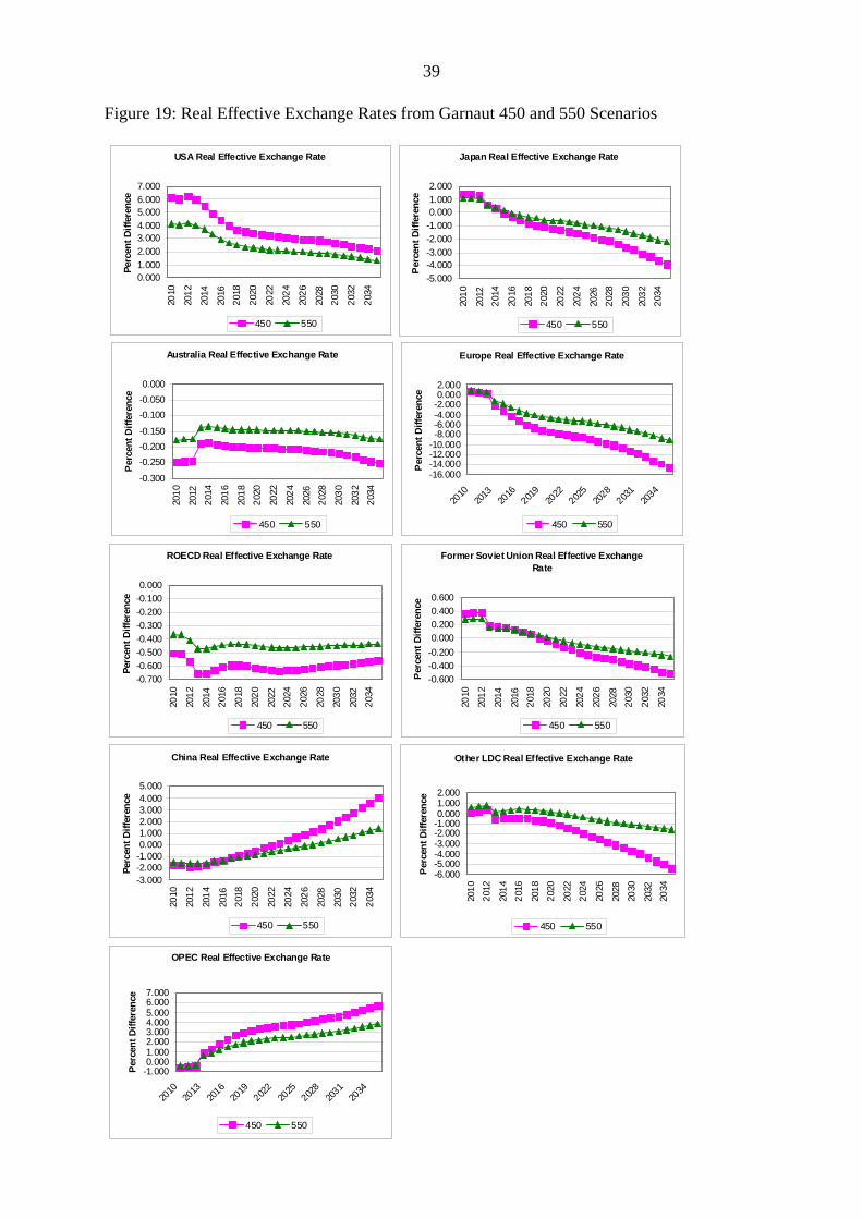
39
Figure 19: Real Effective Exchange Rates from Garnaut 450 and 550 Scenarios
USA Real Effective Exchange Rate
0.0001.0002.0003.0004.0005.0006.0007.000
2010
2012
2014
2016
2018
2020
2022
2024
2026
2028
2030
2032
2034
Perc
ent D
iffer
ence
450 550
Japan Real Effective Exchange Rate
-5.000-4.000-3.000-2.000-1.0000.0001.0002.000
2010
2012
2014
2016
2018
2020
2022
2024
2026
2028
2030
2032
2034
Per
cent
Diff
eren
ce
450 550
Australia Real Effective Exchange Rate
-0.300
-0.250-0.200-0.150
-0.100-0.0500.000
2010
2012
2014
2016
2018
2020
2022
2024
2026
2028
2030
2032
2034
Per
cent
Diff
eren
ce
450 550
Europe Real Effective Exchange Rate
-16.000-14.000-12.000-10.000-8.000-6.000-4.000-2.0000.0002.000
2010
2013
2016
2019
2022
2025
2028
2031
2034
Per
cent
Diff
eren
ce
450 550
ROECD Real Effective Exchange Rate
-0.700-0.600-0.500-0.400-0.300-0.200-0.1000.000
2010
2012
2014
2016
2018
2020
2022
2024
2026
2028
2030
2032
2034
Perc
ent D
iffer
ence
450 550
Former Soviet Union Real Effective Exchange Rate
-0.600-0.400-0.2000.0000.2000.4000.600
2010
2012
2014
2016
2018
2020
2022
2024
2026
2028
2030
2032
2034
Per
cent
Diff
eren
ce
450 550
China Real Effective Exchange Rate
-3.000-2.000-1.0000.0001.0002.0003.0004.0005.000
2010
2012
2014
2016
2018
2020
2022
2024
2026
2028
2030
2032
2034
Perc
ent D
iffer
ence
450 550
Other LDC Real Effective Exchange Rate
-6.000-5.000-4.000-3.000-2.000-1.0000.0001.0002.000
2010
2012
2014
2016
2018
2020
2022
2024
2026
2028
2030
2032
2034
Per
cent
Diff
eren
ce
450 550
OPEC Real Effective Exchange Rate
-1.0000.0001.0002.0003.0004.0005.0006.0007.000
2010
2013
2016
2019
2022
2025
2028
2031
2034
Per
cent
Diff
eren
ce
450 550

40
Figure 20: Real Effective Exchange Rates from CPRS-5 and CPRS-15vScenarios
USA Real Effective Exchange Rate
0.0002.0004.0006.0008.000
10.00012.000
2010
2012
2014
2016
2018
2020
2022
2024
2026
2028
2030
2032
2034
Perc
ent D
iffer
ence
15 5
Japan Real Effective Exchange Rate
-6.000-5.000-4.000-3.000-2.000-1.0000.0001.0002.000
2010
2012
2014
2016
2018
2020
2022
2024
2026
2028
2030
2032
2034
Per
cent
Diff
eren
ce
15 5
Australia Real Effective Exchange Rate
-0.500
-0.400
-0.300
-0.200
-0.100
0.000
2010
2012
2014
2016
2018
2020
2022
2024
2026
2028
2030
2032
2034
Per
cent
Diff
eren
ce
15 5
Europe Real Effective Exchange Rate
-18.000-16.000-14.000-12.000-10.000-8.000-6.000-4.000-2.0000.000
2010
2013
2016
2019
2022
2025
2028
2031
2034
Per
cent
Diff
eren
ce
15 5
ROECD Real Effective Exchange Rate
-1.200-1.000-0.800-0.600
-0.400-0.2000.000
2010
2012
2014
2016
2018
2020
2022
2024
2026
2028
2030
2032
2034
Perc
ent D
iffer
ence
15 5
Former Soviet Union Real Effective Exchange Rate
-1.000-0.800-0.600-0.400-0.2000.0000.2000.400
2010
2012
2014
2016
2018
2020
2022
2024
2026
2028
2030
2032
2034
Per
cent
Diff
eren
ce
15 5
China Real Effective Exchange Rate
-2.000-1.0000.0001.0002.0003.0004.0005.0006.000
2010
2012
2014
2016
2018
2020
2022
2024
2026
2028
2030
2032
2034
Perc
ent D
iffer
ence
15 5
Other LDC Real Effective Exchange Rate
-15.000
-10.000
-5.000
0.000
2010
2013
2016
2019
2022
2025
2028
2031
2034
Per
cent
Diff
eren
ce
15 5
OPEC Real Effective Exchange Rate
-2.0000.0002.0004.0006.0008.000
10.000
2010
2013
2016
2019
2022
2025
2028
2031
2034
Per
cent
Diff
eren
ce
15 5

41
References
Aldy, J. and R. Stavins (eds) (2007), Architectures for Agreement: Addressing Global
Climate Change in the Post-Kyoto World, Cambridge University Press, pp185-208.
Australian Treasury (2008) Australia's Low Pollution Future: The Economics of Climate Change Mitigation 30 October 2008. Commonwealth of Australia.
Bagnoli, P. McKibbin W. and P. Wilcoxen (1996) “Future Projections and Structural Change” in N, Nakicenovic, W. Nordhaus, R. Richels and F. Toth (ed) Climate Change: Integrating Economics and Policy, CP 96-1 , Vienna: International Institute for Applied Systems Analysis, 181-206.
Barrett, S (2008). "A Portfolio System of Climate Treaties." Discussion Paper 08-13, Cambridge, Mass.: Harvard Project on International Climate Agreements, October 2008.
Blanchard O. and S. Fischer (1989) Lectures on Macroeconomics MIT Press, Cambridge MA.
Blanford, G, Richels, R and T. Rutherford (2008). "Revised Emissions Growth Projections for China: Why Post-Kyoto Climate Policy Must Look East." Discussion Paper 08-06, Cambridge, Mass.: Harvard Project on International Climate Agreements, September 2008.
Garnaut, R. (2008). Garnaut Climate Change Review Final Report, Cambridge University Press, Port Melbourne.
Harvard Project on International Climate Agreements (2008) http://belfercenter.ksg.harvard.edu/project/56/harvard_project_on_international_climate_agreements.html?page_id=209
Henderson, D.W., and W. McKibbin (1993), “A Comparison of Some Basic Monetary Policy Regimes for Open Economies: Implications of Different Degrees of Instrument Adjustment and Wage Persistence,” Carnegie-Rochester Conference Series on Public Policy,39, pp 221-317.
Intergovernmental Panel on Climate Change (2007) Climate Change 2007: Synthesis Report, Cambridge University Press, Cambridge.
International Monetary Fund (2008), World Economic Outlook, April.

42
Jaffe, J. and R. Stavins.(2008) "Linkage of Tradable Permit Systems in International Climate Policy Architecture." Discussion Paper 08-07, Cambridge, Mass.: Harvard Project on International Climate Agreements, September 2008
McKibbin, W., Morris, A. and P. Wilcoxen (2008) “Expecting the Unexpected:
Macroeconomic Volatility and Climate Policy”, Discussion Paper 08-16, Cambridge, Mass.: Harvard Project on International Climate Agreements, November 2008 also CAMA working paper 35/2008, The Australian National University
http://www.cama.anu.edu.au/Working%20Papers/Papers/2008/McKibbin_Morris_Wilcoxen_352008.pdf;
McKibbin W. D. Pearce and A. Stegman (2007) “Long Term Projections of Carbon
Emissions” International Journal of Forecasting, vol 23, pp637-653
McKibbin W. , Shackleton R. and P. Wilcoxen (1999) “What to Expect from an International System of Tradeable Permits for Carbon Emissions” Resource and Energy Economics, volume 21, 3, pp 319-346.
McKibbin W.J. and D. Vines (2000) “Modeling Reality: The Need for Both Intertemporal
Optimization and Stickiness in Models for Policymaking” Oxford Review of Economic Policy vol 16, no 4.
McKibbin W. and P. Wilcoxen (1997), “A Better Way to Slow Global Climate Change”
Brookings Policy Brief no 17, June, The Brookings Institution, Washington D.C. . McKibbin W. and P. Wilcoxen (1998) “The Theoretical and Empirical Structure of the G-
Cubed Model” Economic Modelling , 16, 1, pp 123-148 McKibbin, W. J. and P. J. Wilcoxen (2002a), Climate Change Policy After Kyoto: A
Blueprint for a Realistic Approach, Washington: The Brookings Institution. McKibbin, W. J. and P. J. Wilcoxen (2002b), “The Role of Economics in Climate Change
Policy,” Journal of Economic Perspectives, 16(2), pp.107-130.
McKibbin W. and P. Wilcoxen (2007) “A Credible Foundation for Long Term International Cooperation on Climate Change” in Joseph Aldy and Robert Stavins (eds), Architectures for Agreement: Addressing Global Climate Change in the Post-Kyoto World, Cambridge University Press, pp185-208.

43
McKibbin W.J. and P. Wilcoxen (2008) “Building on Kyoto: Towards a Realistic Global Climate Change Agreement”, Lowy Institute Working Paper in International Economics and CAMA working paper 13/2008; http://www.cama.anu.edu.au/Working%20Papers/Papers/2008/ McKibbin_Wilcoxen_132008.pdf
Obstfeld M. and K. Rogoff (1996) Foundations of International Macroeconomics MIT Press, Cambridge MA.
Pearce D. and W. McKibbin (2007) “Two issues in Carbon Pricing: Timing and Competitiveness” Lowy Institute Working Paper in International Economics no 1.07.
Pizer, W.A. (1997), “Prices vs. Quantities Revisited: The Case of Climate Change,”
Resources for the Future Discussion Paper 98-02, Washington: Resources for the Future.
Roberts, M. J., and A. M. Spence (1976), “Effluent Charges and Licenses under
Uncertainty,” Journal of Public Economics, 5, 193-208.
Stern, N. (2006), Stern Review: Report on the Economics of Climate Change. Cambridge University Press, UK.
Taylor, J. B. (1993), Discretion Versus Policy Rules in Practice. Carnegie-Rochester
Carnegie-Rochester Conference Series on Public Policy 39, 195-214. Weitzman, M. L. (1974), “Prices vs. Quantities,” Review of Economic Studies, 41, 477-91.
Weyant, John (ed.) (1999), “The Costs of the Kyoto Protocol: A Multi-model Evaluation,” The Energy Journal, Special Issue.

44
Appendix A; New Treasury Equations:
This appendix should be read in conjunction with the model documentation for version GGGV83E which contains the naming conventions as well as all equations in the model. Please see:
http://www.msgpl.com.au/g3versions.htm

45
Table A1: New Treasury Equations
goods_e: CON = delta_eH * CNPE *
exp( PRCE - PRY - ln(1+cc_ch4G*TCARCH4) )^sigma_eH;
EMME = 1000*( sum( goods, cc_ch4*OUG ) + sum( goods, cc_ch4G*CON ) +
sum( goods, cc_ch4W*OUG ) );
EMNO = 1000*( sum( goods, cc_n2o*OUG ) + sum( goods, cc_n2oW*OUG ) );
EMNC = 1000*( sum( goods, cc_ncc*OUG ) );
EMTC = EMNC + EMIS ;
EMTCEQ = EMTC + EMME + EMNO ;
PRD = ln( sum(sectors, makeinv*(exp(PRP)))
+ carcoef*TCAR + (cc_ch4 + cc_ch4W)*TCARCH4 + (cc_n2o + cc_n2oW)*TCARNO
+ cc_ncc*TCARNC + btucoef*TBFD );
PRCE = cd_eH*sum( goods_e,
delta_eH*(ln(1+cc_ch4G(goods_e)*TCARCH4)+PRY(goods_e)) )
+ (1-cd_eH)*ln( sum(goods_e,
delta_eH*(ln(1+cc_ch4G(goods_e)*TCARCH4)+exp(PRY(goods_e)))^(1-sigma_eH))
) / (1-sigma_eH*(1-cd_eH)) ;
dest: TAXE = sum( goods, (carcoef*TCAR + (cc_ch4 + cc_ch4W)*TCARCH4 +
(cc_n2o + cc_n2oW)*TCARNO
+cc_ncc*TCARNC + btucoef*TBFD)*OUG +
(cc_ch4G *TCARCH4)*CON+
(carcoef*TCEX + btucoef*TBFX)*EXQ +
(carcoef*TCAI + btucoef*TBFI)*IMQ );
TCARCH4 = TCAR;
TCARNO = TCAR;
TCARNC = TCAR;

46