august 2011 working paper - Mercatus Center€¦ · working paper Tax raTes and migraTion By Antony...

working paperTax raTes and migraTion

By Antony Davies and John Pulito

no. 11-31 august 2011

The ideas presented in this research are the authors’ and do not represent official positions of the Mercatus Center at George Mason University.

Tax Rates and Migration

Antony Davies

John Pulito

Top Marginal Income-Tax Rates

In an environment marked by large budget deficits, state “millionaire” taxes have begun

to draw increasing attention. According to financial journalists Robert Frank and Laura

Saunders, “Advocates of the taxes say that with the wealthy riding the recovery of stock markets

and global growth, and with less fortunate Americans facing unemployment and a housing

slump, the top earners can best afford to foot the government’s bills. Opponents say the taxes

amount to a redistribution of wealth and encourage runaway government spending.”1

The term “millionaire tax” does not necessarily mean a tax imposed only on individuals

earning more than a million dollars per year. Depending on the state, landing in the top income-

tax bracket could require earning more than $1 million (New Jersey, Maryland, and California)

or as little as $200,000 (Hawaii and Ohio) or even $150,000 (Arizona). Recent attention has

focused on New Jersey, which increased its (former) top income-tax rate by more than 14

percent (from 8.97 percent to 10.25 percent) in 2009 for individuals making more than $500,000

and added a new 10.75 percent tax bracket for those earning more than $1 million. Top marginal

income tax rates vary widely across states (Figure 1). Figure 2 shows the top income-tax brackets

and the corresponding top income-tax rates for states in which the cutoff for the top bracket

exceeds the median household income for the United States (approximately $50,000). Figure 3

shows changes in top marginal income-tax rates for various states over the recent past.

1 Robert Frank and Laura Saunders, “The Battle of the Millionaire’s Tax,” Wall Street Journal, March 26, 2011.

Figure 1: Top Marginal Tax Rate, Single Payer, 20112

Source: Tax Foundation, State Individual Income Tax Rates, 2000–2011 (Washington, DC: Tax Foundation, March 3, 2011), http://www.taxfoundation.org/taxdata/show/228.html.

Produced by: Davies and Pulito

2 The tax for Tennessee only applies to interest and dividend income.

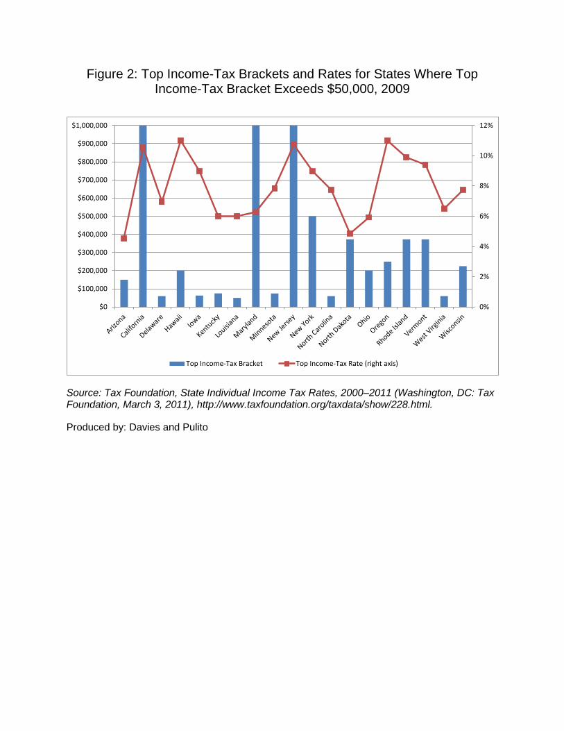
Figure 2: Top Income-Tax Brackets and Rates for States Where Top Income-Tax Bracket Exceeds $50,000, 2009

0%

2%

4%

6%

8%

10%

12%

$0

$100,000

$200,000

$300,000

$400,000

$500,000

$600,000

$700,000

$800,000

$900,000

$1,000,000

Top Income-Tax Bracket Top Income-Tax Rate (right axis)



Figure 3: Changes in the Top Marginal Income-Tax Rate for Single Payers, 2000–20113



3 We only display states that experienced a change in tax rates. If no change occurred, or if a state does not have an income tax, we did not include it. Also, while North Dakota, Rhode Island, and Vermont now have a progressive income-tax system, this was not the case in 2000. As of 2000, these states charged an income tax equal to a certain percentage of the federal income tax liability.

This paper responds to an experiment by Young and Varner, who explore high-income

migration into and out of New Jersey following an increase in the marginal tax rate in 2004.4

Young and Varner look at microdata for New Jersey in the four years preceding and the four

years following the 2004 increase in the top state income-tax rate. They conclude that the

increase had little effect on migration.

Two problems arise from Young and Varner’s study. First, since it looked only at New

Jersey, a coincident factor specific to New Jersey could explain their results. For example, New

York City is atypical in its concentration of high-income jobs. To hold one of these jobs, a

person must live in the vicinity of New York City. Living in New Jersey may be a complement

to working in New York City and so mitigate out-migration from New Jersey. A second and

more troubling problem is technical. Young and Varner model migration on a trinary scale,

where -1 indicates a household that migrated out of New Jersey, 1 indicates a household that

migrated into New Jersey, and 0 indicates a household that did not migrate. They employ

ordinary least squares (OLS) estimation with this trinary measure as the dependent variable. This

procedure is incorrect and will yield, if not biased results, then at least estimators whose

statistical properties are unknown. In short, given the techniques they employed, it is not possible

to make any statistical inference from their data.5

Our research addresses these two problems by comparing changes in top marginal

income-tax rates to migration between the states and counties within the states in a panel data

setting. By examining data over time and across many states and counties, any coincidental

relationships specific to particular counties or particular states are averaged out. We measure

4 C. Young and C. Varner, “Millionaire Migration and State Taxation of Top Incomes: Evidence from a Natural Experiment,” National Tax Journal 64, no. 2 (2011): 255–284. 5 The correct procedure would have been to employ ordered or multinomial logit.

migration as a continuous variable rather than a trinary variable, making OLS procedures the

correct procedures to employ.

Using aggregate data from the Census Bureau for 790 counties across 50 states over the

period 2004 to 2009, we examine the relationship between changes in the top marginal income-

tax rate and changes in the number of high-income households. While these data are useful for

showing the rise and fall in the number of high-income households, they leave two questions

unanswered: (1) how much of the rise and fall is due to normal migration versus movements into

and out of the high-income category, and (2) to which locations are the migrating households

moving? We also look at Statistics of Income data from the IRS that show the origin and

destination of migrants across states. Using these data, we compare changes in relative tax rates

across pairs of states to the ratio of in-migrants to out-migrants across the states. While this data

set includes all households, it allows us to identify changes in the number of households that are

due specifically to migration and to identify the origin and destination of the migration.

Additional research in this area includes that of Conway and Houtenville,6 who find that

the elderly are less likely to move into a state with a high estate tax; Fox et al.,7 who find that an

increase in income-tax rates is associated with a decrease in the likelihood of in-migration;

Bakija and Slemrod, who find that elderly individuals change their state of residence to avoid

high estate and sales taxes;8 and Coomes and Hoyt,9 who find that increases in state-tax rates are

associated with a decline in in-migration.

6 K. S. Conway and A. J. Houtenville, “Elderly Migration and State Fiscal Policy: Evidence from the 1990 Census Migration Flows,” National Tax Journal 51, no. 1 (2001): 103–123. 7 W. F. Fox, H. W. Herzog, and A. M. Schlottman, “Metropolitan Fiscal Structure and Migration,” Journal of Regional Science 29, no. 4 (1989): 523–536. 8 J. Bakija and J. Slemrod, “Do the Rich Flee from High State Taxes? Evidence from Federal Estate Tax Returns” (Working Paper No. 10645, National Bureau of Economic Research, Cambridge, MA, 2004), 1–50.

County-Based Model

We construct two sets of models: county-based models and state-based models. The

county-based model contains data showing the number of high-income households (defined as

households with incomes of $200,000 per year or more) in each of 791 counties over time.10 We

use this model to measure the relationship between marginal income-tax rates and the number of

high-income households. The state-based model contains data showing the number of tax filers

that move from one state to another for each pair-wise combination of states over time. We use

this model to measure the relationship between marginal income-tax rates and migration across

states.

Young and Varner attempt to explain migration as a function of a change in New Jersey’s

income tax only.11 Bakija and Slemrod look at the effects of estate, inheritance, gift, income,

sales, and property-tax rates.12 They control for differences in government expenditures,

population, unemployment, crime, climate, death rates, stock prices, and housing prices. Wallace

attempts to explain migration as a function of differences in tax rates (income, property, and

sales), employment, education expenditures, welfare expenditures, climate, home values, and

high school enrollment.13 Conway and Houtenville look at the distances between geographic

areas; differences in household incomes; crime; climate; education, health, welfare, and

9 P. A. Coomes and W. H. Hoyt, “Income Taxes and the Destination of Movers to Multistate MSAs,” Journal of Urban Economics 63, no. 3 (2008): 920–937. 10 Data come from the Census Bureau’s American Community Survey for each year from 2004 through 2009. The American Community Survey produces one-year estimates annually for counties with a population of 65,000 or more. 11 Young and Varner, “Millionaire Migration.” 12 Bakija and Slemrod, “Do the Rich Flee from High State Taxes?” 13 S. Wallace, “The Effect of State Income Tax Structure on Interstate Migration,” Fiscal Research Program, Report No. 79, 2002. Wallace looks at individual data and so also includes individual-level variables that we cannot include in our aggregated data model.

Medicaid expenditures; and income, property, estate, and gift taxes.14 Lee and Roseman look at

unemployment rates, property taxes, income taxes, climate, and other individual-specific

factors.15 Because we use aggregate data, we have no visibility into individual-specific factors.

We attempt to explain migration as a function of differences in income, property, and sales-tax

rates; income-tax bracket definitions; unemployment rates; crime rates; and climate.16

To control for changes in the total number of high-income households over time as well

as changes in the number of counties reporting across different years, for each year, we look at

the number of high-income households in each county as a fraction of all high-income

households among the reporting counties in that year. An increase in this measure indicates an

increase in that county’s share of high-income households that exist in the given year. To

estimate the effect of changes in each state’s marginal high-income tax rate, for each state, we

look at the marginal income-tax rate that applies to incomes of $200,000.17 Where migration is

concerned, what is important is not the state’s marginal rate but rather the state’s rate relative to

those in other states. Therefore, we scale each state’s tax rate by the average high-income

marginal rate across all states to obtain Rit. The effect of a high income-tax rate can be mitigated

by increasing the minimum income to which the rate applies. To account for this, we include the

lower limit of the tax bracket applicable to those earning $200,000, Bit. Other taxes that may

influence migration are property taxes and sales taxes. For each county, we measure the average

property tax as a percentage of home value and express this as a fraction of the average measure

14 Conway and Houtenville, “Elderly Migration and State Fiscal Policy.” 15 S. Lee and C. C. Roseman, “Migration Determinants and Employment Consequences of White and Black Families, 1985–1990,” Economic Geography 75, no. 2 (1999): 109–133. 16 The latter two factors were highly insignificant in all of our tests, and we excluded them from the results we show. 17 With the exceptions of California, Maryland, New Jersey, New York, North Dakota, Rhode Island, Vermont, and Wisconsin, the state marginal income-tax rate that applies to a $200,000 income is also that state’s top marginal income-tax rate.

across all counties in the data set Pit. Similarly, Sit represents the sales tax in each county as a

fraction of the average for all counties.

To allow for the possibility that the employment climate may influence migration, we

include the unemployment rate in each county as a fraction of the average across all counties

(Uit). One possibility is that the unemployment rate has little effect on migration because

unemployment disproportionately affects the lesser educated, and the lesser educated, on

average, are also less mobile. Another possibility is that the unemployment rate in a county

affects the quality of life in that county for all people (for example, via a less vibrant community,

deterioration of homes, the presence of homeless people and panhandlers); therefore, those who

are more mobile, even though employed, will tend to want to move out of areas in which many

others are unemployed. Including the unemployment rate in the analysis allows for the

possibility of, but does not assume, an unemployment effect.

Finally, there may be other county-specific factors other than those factors we have

identified that influence the number of high-income households. We include dummy variables in

a cross-section fixed effects model to account for these factors. Table 1 defines the variables we

use in the county-based model.

Table 1: Variable Definitions for the County-Based Model

Variable Definition Mean (standard deviation)

Hit

Number of households reporting income over $200,000 in county i in year t expressed as a fraction of all U.S. households in year t

7.80 x 10-6 (7.09 x 10-6)

Rit

The marginal state income-tax rate applicable to a $200,000 income in county i in year t expressed as a fraction of the average, across all states, of the marginal state income-tax rates applicable to a $200,000 income18

0.938 (0.498)

Bit The lower limit of the tax bracket applicable to those earning $200,000 in county i in year t18 41,035 (60,018)

Pit Property tax as a fraction of home value in county i in year t expressed as a fraction of the average for the state

1.000 (0.209)

Sit Sales tax in county i in year t expressed as a fraction of the average U.S. sales tax in year t 0.999 (0.277)

Uit

Unemployment rate in county i in year t expressed as a fraction of the average U.S. unemployment rate in year t

1.001 (0.300)

Equation 1 shows our county-based model. We estimate the model using OLS for panel

data with fixed effects with cluster-robust standard errors. Table 2 shows the results, which

indicate a negative (though weak) relationship between the high-income tax rate and the number

of high-income households. For example, in 2008, Wisconsin’s high-income tax rate was 6.75

percent—1.23 times the average for the country in that year.19 In 2009, the state raised its high-

income tax rate to 7.75 percent, or 1.38 times the average for that year. Our model predicts that

Wisconsin’s share of high-income households should have fallen from 12,070 (or 0.013 percent

18 These data are constant for all counties within a given state. 19 By “the country,” we mean those counties included in our data set for the specified year.

of the total for the country) to 12,020, for a loss of 50 high-income households. In fact, the 22

counties reported for Wisconsin lost a combined 50 high-income households that year.

Equation 1: 1 2 3 4 5it i it it it it it itH R B P S U uα β β β β β= + + + + + +

Table 2: Relationship Between High-Income Households and High-Income Tax Rates

Variable Description Coefficient Estimate (standard deviation)

Hit Number of high-income households

Rit High-income marginal income-tax rate -7.72 x 10-7 (4.48 x 10-7)*

Bit High-income tax bracket cutoff 3.66 x 10-12 (9.89 x 10-13)***

Pit Property-tax rate -1.27 x 10-9 (4.84 x 10-7)

Sit Sales-tax rate -8.88 x 10-7 (6.43 x 10-7)

Uit Unemployment rate -8.78 x 10-7 (2.19 x 10-7)***

County-based data. Panel OLS, fixed cross-sectional, 3,901 observations (791 counties, annual data 2005–2009). Cluster-robust standard errors. * Significant at 10%. ** Significant at 5%. *** Significant at 1%. See table 1 for precise variable definitions.

Figure 4: Prevalence of High-Income Households in Counties with Below- and Above-Median Income Tax Rates (791 counties, 2005–2009)

0.00%

0.02%

0.04%

0.06%

0.08%

0.10%

0.12%

0.14%

0.16%

0.18%

Counties With Below-Median Income-Tax Rates Counties With Above-Median Income-Tax Rates

Coun

ty's

Shar

e of

Hig

h-In

com

e Ho

useh

olds

Source: 2009 American Community Survey 1-Year Estimates, 2008 American Community Survey 1-Year Estimates, 2007 American Community Survey 1-Year Estimates, 2006 American Community Survey, 2005 American Community Survey, 2004 American Community Survey. American FactFinder, (Washington, DC: Census Bureau, 2005- 2009)(http://factfinder.census.gov/servlet/DownloadDatasetServlet?_lang=en).


Figure 4 compares the average county’s share of high-income households for counties

with state marginal high-income tax rates above and below the median for each year.20 Counties

with below-median high-income tax rates had 0.16 percent of the high-income households for

each year versus 0.13 percent for counties with above median high-income tax rates—a 22

20 The median state income tax was 6 percent in each year.

percent difference.21 Figure 5 shows a similar analysis for the counties broken into high-income

tax rate quartiles. Quartiles one through three exhibit the inverse relationship between the high-

income tax rate and counties’ shares of high-income households: as the high-income tax rate

rises, counties’ shares of high-income households decline. The fourth quartile is an exception,

showing a greater share of high-income households.22

Figure 5: Prevalence of High-Income Households in Counties with Different Income-Tax Rates (791 counties, 2005–2009)

0.00%

0.02%

0.04%

0.06%

0.08%

0.10%

0.12%

0.14%

0.16%

0.18%

0.20%

Lowest-Income Quartile Second Quartile Third Quartile Highest-Income Quartile

Coun

ty's

Shar

e of

Hig

h-In

com

e Ho

useh

olds

Source: 2009 American Community Survey 1-Year Estimates, 2008 American Community Survey 1-Year Estimates, 2007 American Community Survey 1-Year Estimates, 2006 American Community Survey, 2005 American Community Survey, 2004 American Community Survey. American FactFinder, (Washington, DC: Census Bureau, 2005 2009)(http://factfinder.census.gov/servlet/DownloadDatasetServlet?_lang=en).


21 The difference is statistically significant with p < 0.001. 22 Differences are all pair-wise statistically significant with p < 0.001, with the exception of the difference between the second and fourth quartiles, which is significant with p < 0.05.

Using equation 1, we find a positive relationship between the lower limit of the high-

income tax bracket and a county’s share of high-income households. This finding is consistent

with our findings for the high-income tax rate. As the lower limit of the high-income tax bracket

increases, fewer “near” high-income households are subject to the high-income tax bracket

(where a “near” high-income household is one that is in the tax bracket directly below the high-

income tax bracket). An impact on near high-income households might affect a county’s share of

high-income households because households that are not high-income but which expect to

become high-income will, on average, avoid counties with higher high-income tax rates.

Our estimates of equation 1 show no significant relationship between property- and

income-tax rates and the share of high-income households. We do find a negative relationship

between a county’s unemployment rate and the county’s share of high-income households. This

relationship is predictable and the causality likely runs in both directions: people with high-

incomes will tend not to want to reside in areas of high unemployment and areas of high

unemployment will tend not to generate high incomes.

State-Based Model

The drawback to the county-based model is that while it shows changes in the number of

high-income households, it does not show movements in households across states. In other

words, a change in the number of high-income households could be due to migration or it could

be due to a change in households’ incomes. We also examine migration data from the IRS’s

Statistics on Income that show movements of households between states.23 For each state in each

year, the data show the number of households that moved from that state to each of the other 49

23 For simplicity, we continue to speak in terms of households. Technically, the IRS data measure tax returns.

states and the number of households that moved from each of the other 49 states to that state.

Our data set spans the years 2006 through 2009. Accounting for pair-wise movements between

states, we have a possible 10,000 observations. Unlike our county-based models, the state-based

model shows migration of all households, not only high-income households. However, in

keeping with our focus on the effect of changes in high-income marginal tax rates, we will

examine the relationship between high-income marginal tax rates and the migration of all

households.

To account for the direction of migration, each variable contains three subscripts that

represent the state of origin, the state of destination, and the year, respectively. For example, Mijt

is the ratio of migrants moving from state j to state i to the number moving from state i to state j.

It is helpful to think of state i as the “home state.” A ratio greater than one indicates a net inflow

of households from state j to the home state. ΔRijt is the difference in high-income marginal state

income-tax rates for state j versus the home state, where a positive number indicates that state j’s

tax rate is higher than the home state’s tax rate. Table 3 shows the variable definitions.

Table 3: Variable Definitions for the State-Based Model

Variable Definition Mean (standard deviation)

Mijt

For year t, the number of migrants moving from state j to state i divided by the number moving from state i to state j. For state i, this is the ratio of “in-migrants” to “out-migrants.”

1.035 (0.323)

ΔRijt

For year t, the marginal state income-tax rate applicable to a $200,000 income in state j minus the marginal state income-tax rate applicable to a $200,000 income in state i.

0.001 (0.039)

ΔBijt

For year t, the lower limit of the tax bracket applicable to a $200,000 income in state j minus the lower limit of the tax bracket applicable to a $200,000 income in state i.

0.000 (82,324)

ΔPijt For year t, property tax as a fraction of home value in state i minus property tax as a fraction of home value in state j.

0.000 (0.020)

ΔSijt For year t, sales tax in state i minus sales tax in state j. 0.000 (0.026)

To the extent that tax rates influence migration, what matters is the difference in tax rates

between the origin and destination states. To adjust for differences in population size, we look at

the ratio of households entering state X from state Y (“in-migrants”) to those leaving state X for

state Y (“out-migrants”). If we think of state i as the home state, then a positive tax difference

means that taxes are higher outside the home state. If tax rates affect migration, we would expect

to see a positive relationship between the tax differences and the migration ratio. That is, as other

states’ tax rates rise relative to the home state, the home state should experience a net in-

migration from those other states. Equation 2 shows our model. To account for state-specific

migration effects, we include dummies representing the home states. Table 4 shows the results.

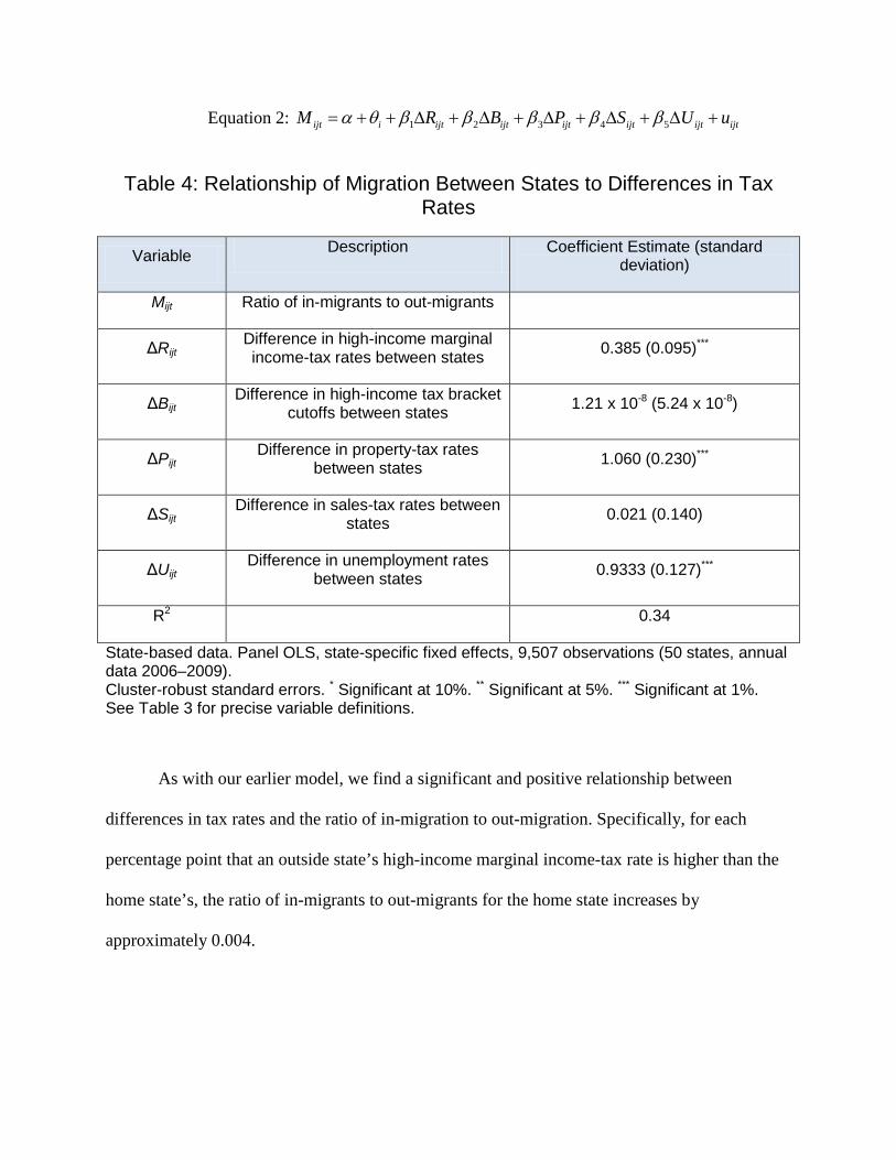
Equation 2: 1 2 3 4 5ijt i ijt ijt ijt ijt ijt ijtM R B P S U uα θ β β β β β= + + ∆ + ∆ + ∆ + ∆ + ∆ +

Table 4: Relationship of Migration Between States to Differences in Tax Rates

Variable Description Coefficient Estimate (standard deviation)

Mijt Ratio of in-migrants to out-migrants

ΔRijt Difference in high-income marginal income-tax rates between states 0.385 (0.095)***

ΔBijt Difference in high-income tax bracket

cutoffs between states 1.21 x 10-8 (5.24 x 10-8)

ΔPijt Difference in property-tax rates

between states 1.060 (0.230)***

ΔSijt Difference in sales-tax rates between

states 0.021 (0.140)

ΔUijt Difference in unemployment rates

between states 0.9333 (0.127)***

R2 0.34

State-based data. Panel OLS, state-specific fixed effects, 9,507 observations (50 states, annual data 2006–2009). Cluster-robust standard errors. * Significant at 10%. ** Significant at 5%. *** Significant at 1%. See Table 3 for precise variable definitions.

As with our earlier model, we find a significant and positive relationship between

differences in tax rates and the ratio of in-migration to out-migration. Specifically, for each

percentage point that an outside state’s high-income marginal income-tax rate is higher than the

home state’s, the ratio of in-migrants to out-migrants for the home state increases by

approximately 0.004.

Figure 6: Migration Between States with Below- and Above-Median Differences Income-Tax Rates (1,250 pair-wise combinations of states,

2009)

0.98

1.00

1.02

1.04

1.06

1.08

1.10

Tax Difference Between States Is Below Median Tax Difference Between States Is Above Median

Ratio

of I

n-M

igra

nts

to O

ut-M

igra

nts

Source: State-to-State Inflow 2008-2009, State-to-State Outflow 2008-2009. Internal Revenue Service, SOI Tax Stats: State-to-State Migration Database Files (Washington, DC: IRS, 2009), http://www.irs.gov/taxstats/article/0,,id=212702,00.html.


Figure 6 compares migration ratios between states that exhibit large and small differences

in high-income marginal tax rates. The bar on the left shows that when there is less difference in

high-income marginal tax rates between states, migration between the states tends to be lower.

The bar on the right shows that when the difference in tax rates is large, migration tends to be

higher, with the net migration flowing from the higher-tax states to the lower-tax states.24 Figure

24 The difference is significant at p < 0.001.

7 shows a similar analysis across high-income tax rate quartiles.25 With the exception of the first

quartile (where the difference in high-income tax rates is the least, and often zero), as the

difference in high-income tax rates increases across states, there is a significant increase in the

migration ratio between the states—again, with households flowing from higher-tax states to

lower-tax states.

Figure 7: Migration Between States with Various Differences in Income-Tax Rates (1,250 pair-wise combinations of states, 2009)

0.94

0.96

0.98

1.00

1.02

1.04

1.06

1.08

1.10

1.12

1.14

Lowest-Income Quartile Second Quartile Third Quartile Highest-Income Quartile

Ratio

of I

n-M

igra

nts

to O

ut-M

igra

nts

Source: State-to-State Inflow 2008-2009, State-to-State Outflow 2008-2009. Internal Revenue Service, SOI Tax Stats: State-to-State Migration Database Files (Washington, DC: IRS, year), http://www.irs.gov/taxstats/article/0,,id=212702,00.html. Produced by: Davies and Pulito

It is noteworthy that we observe a significant effect even though we are comparing the

migration of all households to the marginal income-tax rate applied to high-income households.

25 The difference between any two quartiles is significant at p < 0.02.

There are at least three possible explanations. One is that higher-income households are more

mobile and so the majority of migration involves high-income households. If this is the case,

then our results speak directly to the relationship between high-income tax rates and high-income

migration. A second possible explanation is that people who anticipate earning higher incomes

take account of high-income tax rates. A third and related explanation is that all households take

the top tax rate as a signal for the state’s proclivity for raising taxes in general. In other words, a

state that is more likely to raise taxes on high-income households is also more likely to lower the

threshold of “high-income” households to include middle-income households.

Of additional concern is the direction of causality. Do higher taxes encourage out-

migration, or does increased out-migration pressure states to increase tax rates in an attempt to

make up for lost revenues due to the out-migration? We conducted Granger causality tests on the

state data and found strong (p < 0.001) bi-directionality in causality between migration and the

top marginal income-tax rate, and between migration and the top marginal income-tax bracket.

These results suggest a feedback loop in which higher tax rates (or lowered top tax brackets) lead

to out-migration which, in turn, pressures states to raise tax rates (or lower top brackets). We find

strong evidence (p < 0.001) that changes in property-tax rates drive changes in migration, but

weaker evidence (p = 0.07) that changes in migration drive changes in property-tax rates.

Finally, we find strong evidence (p < 0.001) that changes in sales-tax rates drive changes in

migration but no evidence (p = 0.73) that changes in migration drive changes in sales-tax rates.

Conclusion

This paper explores the relationship between high-income tax rates and the interstate

migration of high-income households. Controlling for property-tax rates, sales-tax rates, high-

income tax brackets, unemployment, and state/county-specific and time-specific effects, we find

that higher state income-tax rates cause a net out-migration not only of higher-income residents,

but of residents in general. We also find that changes in the income levels to which the tax rates

apply similarly affect out-migration. For county-level data, we find that high-income households

react to a lowering of income levels to which higher tax rates apply in the same way that they

react to increases in the tax rates themselves. This behavior suggests that the tendency to lower

the threshold for “high income” or “millionaire” households to capture households that are not

millionaires may entice those households to follow the behavior of millionaire households and

flee to more tax-friendly environs. Finally, for state-level data, we find that the effect of property

taxes on migration is significantly stronger than the effect of high-income tax rates on migration.

For example, a one percentage point increase in the property-tax differential between two states

has almost three times the effect on migration as does a one percentage point increase in the

difference in high-income tax rates. All of these data suggest a recipe for population depletion.

States lose households to more tax-friendly states by (1) lowering the “high-income” threshold

so as to capture more households, (2) increasing high-income tax rates, and (3) increasing

property-tax rates.

august 2011 working paper - Mercatus Center€¦ · working paper Tax raTes and migraTion By Antony...

Documents

Transcript of august 2011 working paper - Mercatus Center€¦ · working paper Tax raTes and migraTion By Antony...