AUFLS Scheme Design Technical Summary - … Scheme Design Technical Summary 07 August 2013 IMPORTANT...
64
AUFLS Scheme Design Technical Summary 07 August 2013
-
Upload
phamkhuong -
Category
Documents
-
view
217 -
download
0
Transcript of AUFLS Scheme Design Technical Summary - … Scheme Design Technical Summary 07 August 2013 IMPORTANT...

AUFLS Scheme Design
Technical Summary
07 August 2013

IMPORTANT
Disclaimer
The information in this document is provided in good-faith and represents the opinion of Transpower
New Zealand Limited, as the System Operator, at the date of publication. Transpower New Zealand
Limited does not make any representations, warranties or undertakings either express or implied, about
the accuracy or the completeness of the information provided. The act of making the information
available does not constitute any representation, warranty or undertaking, either express or implied.
This document does not, and is not intended to; create any legal obligation or duty on Transpower New
Zealand Limited. To the extent permitted by law, no liability (whether in negligence or other tort, by
contract, under statute or in equity) is accepted by Transpower New Zealand Limited by reason of, or in
connection with, any statement made in this document or by any actual or purported reliance on it by
any party. Transpower New Zealand Limited reserves all rights, in its absolute discretion, to alter any of
the information provided in this document.
Copyright
The concepts and information contained in this document are the property of Transpower New Zealand
Limited. Reproduction of this document in whole or in part without the written permission of Transpower
New Zealand.
Contact Details
Address: Transpower New Zealand Ltd
96 The Terrace
PO Box 1021
Wellington
New Zealand
Telephone: +64 4 495 7000
Fax: +64 4 498 2671
Email: [email protected]
Website: http://www.systemoperator.co.nz

SYSTEM OPERATOR REPORT: AUFLS FRAMEWORK SUMMARY
3
Contents 1. Executive Summary ...................................................................................... 4 2. Introduction ................................................................................................ 7
Glossary of Terms ..................................................................................... 7 2.1
Background .............................................................................................. 8 2.2
Purpose ................................................................................................. 10 2.3
3. Scheme Design Principles ............................................................................ 10 Objective of AUFLS Scheme ...................................................................... 10 3.1
Limiting Factors ...................................................................................... 11 3.2
4. Baseline Requirement ................................................................................. 11 Methodology ........................................................................................... 12 4.1
Findings ................................................................................................. 12 4.2
5. Alternate Scheme Designs ........................................................................... 13 Base schemes (frequency and time) .......................................................... 13 5.1
Variants on the base scheme .................................................................... 13 5.2
6. Test Methodology ....................................................................................... 15 Overview of AUFLS Scheme Performance ................................................... 15 6.1
7. Performance Criteria ................................................................................... 18 Weighting (Probability) ............................................................................ 19 7.1
Case Scaling ........................................................................................... 19 7.2
Scoring Metric ......................................................................................... 19 7.3
8. Results...................................................................................................... 21 Base Schemes (Fixed Frequency and Time) ................................................ 21 8.1
Faster Operating Time ............................................................................. 23 8.2
Use of Rate of Change of Frequency (RoCoF) .............................................. 24 8.3
Findings ................................................................................................. 25 8.4
9. Analysing Provision Behaviour ...................................................................... 25 10. Proposal Factors ......................................................................................... 29
Cost-Benefit Analysis ............................................................................... 30 10.1
11. Summary of Findings and Recommendations ................................................. 32 12. Links to additional information ..................................................................... 33 13. Appendix A: Probability Distribution Methodology ........................................... 34 14. Appendix B: Operating Time ........................................................................ 37 15. Appendix C: Use of Rate of Change of Frequency (RoCoF) Relays ..................... 39
Settings ................................................................................................. 39 15.1
Scheme design ....................................................................................... 43 15.2
Other features ........................................................................................ 44 15.3
Specification and performance requirements ............................................... 45 15.4
16. Appendix D: AUFLS Requirement Changes Cost Benefit Analysis ...................... 47 Purpose ................................................................................................. 47 16.1
Instantaneous Reserve procurement cost ................................................... 48 16.2
AUFLS Load Shedding Costs ..................................................................... 54 16.3
Relay costs ............................................................................................. 61 16.4
Frequency Collapse Cost .......................................................................... 62 16.5
Summary of key messages ....................................................................... 63 16.6

SYSTEM OPERATOR REPORT: AUFLS FRAMEWORK SUMMARY
4
1. EXECUTIVE SUMMARY
AUFLS is the acronym for Automatic Under-Frequency Load Shedding and describes the
set of relays in New Zealand which automatically trip blocks of load following a severe
under-frequency event so as to restore the system frequency.
The System Operator relies on these relays to prevent system collapse following under-
frequency events which have the potential to cause a system blackout.
New Zealand’s current AUFLS scheme is made up of a minimum of two 16% blocks in
each island. This means that 32% of customer load can automatically disconnect to
restore stability to the power system.
As a significant review of the AUFLS arrangements had not been completed since their
installation in 1965, the System Operator completed a series of technical and economic
reviews of the AUFLS arrangements to identify if the scheme provided adequate
coverage for New Zealand and investigate potential improvements.
The technical reviews indicated that the current two block AUFLS scheme with the
assistance of under-frequency reserve products will prevent under-frequency system
collapse from large defined risks, such as the sudden disconnection of both poles of the
HVDC link.
However, the results provided the System Operator insufficient confidence in the range
of undefined larger “other” risks that can be covered by the AUFLS scheme. The results
highlighted the need for a methodology to determine a reasonable level of coverage and
the amount of load required to provide this coverage level.
Further, the reviews indicated that the current North Island AUFLS arrangements can
result in tripping more AUFLS than required for both defined and undefined events –
leading to dangerous over-frequency conditions and potential system collapse.
In total, the reviews suggest adjusting the current North Island AUFLS arrangements to
improve the reliability of supply from the power system.
To improve overall performance and therefore reliability of the scheme, the System
Operator identified dividing the AUFLS load into more blocks of smaller sizes. The
investigations also indicated the scheme’s performance could further improve through
using the rate of frequency fall to trigger AUFLS.
However, further investigation into the use of the rate of change of frequency (RoCoF)
relay technology found that due to the lack of uniformity in the relay calculation methods
and their susceptibility to inaccuracy, adequate precautions would need to be taken in
their use.
Due to the risk associated with relying on the current North Island AUFLS scheme, the
System Operator sought to propose an implementable AUFLS scheme design in light of
the current limitations and improvement options identified in the previous reports.

SYSTEM OPERATOR REPORT: AUFLS FRAMEWORK SUMMARY
5
The System Operator, with the support of the Electricity Authority, set out through this
technical review to answer the following questions in regards to the North Island AUFLS:
1. What is a reasonable level of AUFLS coverage for the North Island power system?
2. How much load should be allocated to the AUFLS scheme to achieve this coverage
level?
3. What implementable scheme design will more effectively use the load allocated to
the AUFLS scheme?
4. What RoCoF settings will enable prudent introduction of RoCoF relays in New
Zealand?
The System Operator determined a methodology to identify a reasonable level of
coverage of the North Island power system and provide a better view of scheme
performance across a range of events.
The following key findings and recommendations came out of the technical review:
AUFLS provision behaviour impacts the desired AUFLS requirement level
The review indicated that the provision behaviour of AUFLS providers can
significantly impact the performance of the AUFLS scheme, specifically any
practice that results in significant surplus of AUFLS feeders armed. The
outcomes of the Electricity Authority’s Extended Reserves Procurement review
will shape the structure and level of the AUFLS Requirement.
Allocating 32% demand to AUFLS provides a prudent coverage level
The results indicated that within the current limitations, and assuming static
AUFLS provision, a 32% requirement provides a prudent coverage level across
the scenarios assessed.
A ‘large early’ four block scheme design provides effective coverage
A four block scheme made respectively of 10%, 10%, 6%, and 6% provided the
most effective coverage of the implementable scheme designs considered.
Reducing the requirement may be necessary to manage surplus
provision
If the practice of surplus AUFLS allocation continues after any changes to the
AUFLS procurement methods, then the System Operator may recommend
reducing the minimum AUFLS requirement to 26% and adjusting the scheme
design to four blocks made of 8%, 8%, 5%, and 5% respectively. This is
because surplus provision of AUFLS can cause system collapse from over-
frequency following an AUFLS event. Thus, by setting the minimum obligation at
a lower level the System Operator intends to balance the periods of surplus
provision with periods of minimum provision to attempt to get the best overall
level of system security.

SYSTEM OPERATOR REPORT: AUFLS FRAMEWORK SUMMARY
6
An incremental approach to the use and settings of RoCoF relays is
recommended
The analysis indicated that using RoCoF relays benefits the performance of the
scheme. To minimise the risk associated with using unproven technology it is
recommended that only the fourth block, the least likely block to operate, of the
scheme be armed with RoCoF settings. Further it is recommended that
conservative settings be used to only rely on the relay for high impact low
probability events. Therefore the System Operator recommended using the
highest performing frequency and time scheme design and adding on the RoCoF
functionality to the last block as a prudent introduction to the technology.
Future investigation should be given to the use of over-frequency
reserves in relation to AUFLS
The analysis demonstrated that within the current design limitations all of the
schemes assessed result in some level of over-shedding and over-frequency
risk. The use of over-frequency reserves, particularly during the day, could be
used to improve system reliability. However further investigation is into how the
over-frequency arrangements should be modified in the light of related
developments (AUFLS, HVDC, and others) is required and will be carried out as a
part of the UFM project.
The analysis identified that future performance improvements could be made once
greater confidence in the use of RoCoF relays is gained. Further improvements can be
made from reducing the operating time of the AUFLS relay to circuit breaker
configurations. The technical investigation aimed to identify an improvement to the
status quo that can be implemented in the near future.
The proposed scheme design, even with a reduced minimum requirement (26%), is
estimated to deliver improved performance in system collapse cost resulting in savings of
$11m/yr over the status quo scheme. The implementation costs, estimated at $6m, are
well below the break-even cost, estimated at $100m, and therefore the proposal is
considered to be for the long-term benefit of the consumer.
The proposed AUFLS scheme provides greater reliability than the existing scheme and it
is recommended that changing to the proposed scheme design is made as soon as
practicable. The question, what is the most efficient way of securing the AUFLS load for
the long term benefit of the consumer however remains, and the work that the System
Operator and Authority are currently undertaking will answer that question.
The System Operator will be presenting and discussing the contents of this proposal at
the upcoming System Operator workshops in September 2013.

SYSTEM OPERATOR REPORT: AUFLS FRAMEWORK SUMMARY
7
2. INTRODUCTION
GLOSSARY OF TERMS 2.1
AUFLS Automatic Under-Frequency Load Shedding
Automatic shedding of electrical load when the frequency falls below
pre-set frequency levels as specified in the Code.
Bi-pole Both poles of the HVDC link are commonly referred to as the bi-pole
CE Contingent Event
Events that could happen relatively frequently or cause a severe
enough impact on the power system to justify incorporating pre-event
mitigating measures into the scheduling and dispatch processes.
Examples of such measures are instantaneous reserves or security
constraints
df/dt Rate of change of frequency
The rate at which the frequency falls following the loss generation
injecting into the system is referred to as df/dt.
Disturbance The term “disturbance” is used to reference events which remove net
injection from the system causing under-frequency events
ECE Extended Contingent Event
Events that may have a severe impact on the power system but the
likelihood of them occurring is too low to justify implementing any
mitigating measures in planning time.
In such cases, reliance may be placed on demand shedding (AUFLS) to
avoid power system collapse.
RoCoF Rate of change of frequency
In this report, the RoCoF abbreviation is used in reference to the relays
that are capable of shedding load when the frequency fall reaches a set
a speed
TSAT Transient Stability Analysis Tool
The simulation tool used by the System Operator to assess the dynamic
behaviour of the power system. In terms of this report, the tool is used
to assess the behaviour of the system, particularly the frequency,
during under-frequency events.

SYSTEM OPERATOR REPORT: AUFLS FRAMEWORK SUMMARY
8
BACKGROUND 2.2
Purpose of AUFLS
AUFLS is the acronym for Automatic Under-Frequency Load Shedding and describes the
set of relays in New Zealand which automatically trip blocks of load following a severe
under-frequency event to seek to restore the system frequency.
These relays are relied upon by the System Operator to prevent the collapse of the
system following under-frequency events which have the potential to cause a system
blackout.
New Zealand’s current AUFLS scheme is made up of a minimum of two 16% blocks in
each island. This means that 32% of customer load can be automatically disconnected to
restore stability to the power system.
While any AUFLS scheme is designed to prevent system collapse from under-frequency
events, like any such scheme, have limitations in the range of event sizes they can cover
to prevent system blackout.
The original AUFLS arrangement (2 x 20%) was designed with commissioning of HVDC
Pole 1 in 1965 with only one significant review occurring since its installation. This
review reduced the block sizes (2 x 16%), with the introduction of a fast emergency
response product (FRED).
In 2010, the System Operator completed a technical review of the AUFLS arrangements
to determine if the scheme provided adequate coverage for New Zealand. The results of
the technical review concluded that the under-frequency products managed through the
Reserve Management Tool (RMT) and that are available for dispatch should at all times
prevent system collapse from large defined risks, such as the sudden disconnection of
the HVDC bi-pole.
However, the results provided the System Operator insufficient confidence in the range
of undefined larger “other” risks that can be covered by the AUFLS scheme and
highlighted the need to identify the risks which are reasonable to cover.
In 2012, the System Operator developed an AUFLS framework consisting of a Standard,
a Requirement and a Scheme Design. At industry workshops held in the latter part of
2012, the System Operator proposed defining the purpose of AUFLS as being “to manage
a reasonable loss of net injection which results in the frequency dropping below 48 Hz”.
In addition, the establishment of a cyclic review process to determine the reasonable
coverage level was also proposed. This proposal is known as the “AUFLS Standard”.
As the current AUFLS arrangements are largely based on historical practice, several
parties from industry also expressed concern over the technical justification for the
current amount of load allocated to the AUFLS system (32%).
The System Operator set out in this technical review to identify the reasonable level of
coverage the system requires and the required amount of load allocated to AUFLS
scheme to achieve it efficiently. This is known as the AUFLS Requirement.
Scheme Performance
The 2010 technical review and recent analysis completed for the HVDC Pole 3
commissioning demonstrated that operation of the current AUFLS scheme could result in
over-frequency and potentially system collapse from some of the defined risks.

SYSTEM OPERATOR REPORT: AUFLS FRAMEWORK SUMMARY
9
The technical review indicated that the combination of block sizes, the speed of
disconnection, and frequency settings can result in more AUFLS tripping than is required.
This can lead to dangerous over-frequency conditions and the potential for cascade
tripping of generators, which causes a further under-frequency event and, without any
AUFLS remaining, system collapse.
Further, the analysis completed from the HVDC Pole 3 commissioning also indicated that
the dynamic nature of AUFLS provision (the percentage of AUFLS provided during times
of day/week/year) can significantly impact the performance of a scheme.
Together, the results of the technical review and recent Pole 3 analysis outlined the
potential risk associated with the on-going use of the current AUFLS arrangements and
underlined the need for a more robust analysis method to review the overall
performance of an AUFLS scheme.
Considering the need to replace the current scheme and the problems associated with its
design, the System Operator set out to identify an implementable scheme design which
would improve the overall performance of AUFLS and could be an incremental step
toward future scheme improvements.
The work for defining the most efficient way of securing the AUFLS load for the long term
benefit of the consumer is underway, and should provide a procurement method that is
implementable, and supportive of the Authority’s Code amendment principles
Use of Rate of Change of Frequency (RoCoF) Relays
After the 2010 technical review, the System Operator evaluated the costs and benefits
associated with technically feasible options identified in the review. All the options
included increasing the number of AUFLS blocks and one of the options proposed
included the use of rate-of-change-of-frequency (RoCoF) relays.
The economic analysis revealed that the scheme using RoCoF elements resulted in the
largest benefit range for the North Island. The results of the economic analysis were
presented to industry in August 2011 and industry feedback was received on the
proposed changes.
Bench testing was then carried out to ensure RoCoF relays would perform reliably over a
range of system disturbances that would not normally result in AUFLS operation. The
bench testing indicated that while the relays performed within the specified accuracy
margins for clean frequency decays, they are susceptible to calculation inaccuracy due to
system oscillations.
Further, the tests demonstrated that the sampled RoCoF relays all behave differently
when subjected to identical inputs and the unique calculation methods result in a range
of accuracy.
To improve the resilience to system oscillations, the System Operator recommended the
use of a time (hold) delay requirement to minimize the risk of mal-operation (tripping for
events which do not require AUFLS).
In light of the testing work, the System Operator decided that an incremental approach
to using RoCoF relays would be prudent to provide greater practical experience of the
relay performance in New Zealand power system. The System Operator set out to
identify the settings that will enable prudent use of RoCoF.

SYSTEM OPERATOR REPORT: AUFLS FRAMEWORK SUMMARY
10
PURPOSE 2.3
The System Operator, with the support of the Electricity Authority, set out through this
technical review to answer the following questions in regards to the North Island AUFLS1:
What is a reasonable level of AUFLS coverage for the North Island power
system?
How much load should be allocated to the AUFLS scheme to achieve this
coverage level?
How to improve the method of assessing the over-all performance (under and
over-frequency risk) of an AUFLS scheme?
What implementable scheme design will more effectively use the load allocated
to the AUFLS scheme?
What RoCoF settings will enable prudent introduction of RoCoF relays in New
Zealand?
3. SCHEME DESIGN PRINCIPLES
OBJECTIVE OF AUFLS SCHEME 3.1
The purpose of the AUFLS scheme is to manage a reasonable loss of net injection (which
includes both events classified as ECE and Other Events) which would result in the
frequency dropping below 48 Hz.
The ideal AUFLS scheme maximizes the prevention of system collapse from under-
frequency events while minimising the risk of system collapse from over-frequency
following AUFLS operation.
To develop and assess AUFLS schemes, the System Operator identified criteria for the
successful management of a reasonable loss of net injection.
The success criteria of the AUFLS scheme were outlined as follows:
The operation of the scheme should result in the system frequency staying
within the frequency standards specified in the Principle Performance Obligations
(PPO’s) (i.e. not falling below 47 Hz or rising above 52 Hz).
The scheme should be robust enough to maintain the frequency standards for
different load and system configurations (i.e. HVDC in and out service).
The scheme should not operate for contingent events (CE).
The proposed scheme settings must be achievable through commercially
available relays.
It was noted that AUFLS is designed as an under-frequency mitigation measure. There
are events classified as Extended Contingent Events (ECEs) which may result in other
types of power system issues2 (such as voltage instability, islanding or grid
splits/reconfigurations). Although the triggering of AUFLS may contribute to their
management, the scheme is not designed to manage or address these “non” under-
frequency events.
1 Changes to the South Island scheme design were proposed in the previous AUFLS Review found here:
http://www.systemoperator.co.nz/f5573,75968707/Automatic-under-frequency-load-shedding-RoCoF-testing-summary-web.pdf 2 For example, the loss of an interconnecting transformer.

SYSTEM OPERATOR REPORT: AUFLS FRAMEWORK SUMMARY
11
It was also considered that the proposed scheme design should not rely on the use of
Over-Frequency Reserves to improve performance of the status quo scheme design3.
LIMITING FACTORS 3.2
The system frequency is allowed to drop to 48 Hz following a contingent event (e.g. the
loss of a single generator unit). The frequency target following contingent events limits
the maximum allowable frequency for an AUFLS block to trip is 47.9 Hz.4 Previous work
demonstrated that increasing the CE Limit incurred significant instantaneous reserve
procurement cost to industry and therefore was not pursued further.5
The time it takes for protection relays to sense a change system frequency, send a trip
signal and for the circuit breaker to disconnect is known as the AUFLS operating time.
The operating time of the AUFLS trip configurations is currently required to disconnect
load within 400ms of the system frequency reaching the block trigger set point.
At 47 Hz, many North Island generators will trip on under-speed protection, so after
taking into account relay and breaker operating times, the lowest realistic AUFLS setting
is in the range of 47.2 to 47.3 Hz.
The small frequency range of 0.7 Hz combined with the relatively long delay of 400ms
means that there is little scope for greatly increasing the number of blocks or
optimization by arranging the tripping frequencies of the AUFLS blocks. The tripping
frequencies for most schemes studied in this report were fixed at intervals of 0.2 Hz
starting from 47.9 Hz in order to expedite testing and design.
As highlighted in previous reports, increasing the size of the AUFLS frequency band can
enable future improvements to the scheme design. This report will consider whether
changes to the operating times might also offer areas to improve.
4. BASELINE REQUIREMENT
The current AUFLS block arrangements are largely based on historical practice, and
several industry parties have expressed concern over the technical justification for the
current amount of load allocated to the AUFLS system (32%).
The System Operator set out to complete a high level assessment of how much load is
appropriate to allocate to the AUFLS scheme. The requirement was considered a
“baseline”, as further assessment would be carried out after appraising alternative
scheme designs to observe the impact scheme design has on the AUFLS requirement.
3 This is not to say over-frequency reserves could not be used to improve performance, but the scheme design
should not depend on their availability. 4 Note this is for frequency and time triggering and does not include RoCoF triggering 5 See Economic Review found here http://www.systemoperator.co.nz/aufls.

SYSTEM OPERATOR REPORT: AUFLS FRAMEWORK SUMMARY
12
METHODOLOGY 4.1
The methodology involved undertaking a high level assessment aimed at observing the
impact the AUFLS Requirement has on scheme capability and performance. To focus on
the impact of the Requirement, a fixed scheme design was established. The fixed design
was made up of four equal blocks for each requirement level (i.e. 32% resulted in a
4x8% scheme).
The assessment varied the requirement level from 24% to 48% as outlined in Table 1.
Table 1. Requirement levels and scheme designs
Requirement Scheme Design
24% 4x6%
28% 4x7%
32% 4x8%
40% 4x10%
48% 4x12%
Scenarios were created around three load scenarios (peak, med, and low) for three
representative types of event: site loss, sympathetic trip, and ECE. The events were
represented as follows:
Site loss: Huntly Site (U1-5) and Huntly Station (U1-4)
Sympathetic Trip: 2 CCGT’s and Bipole + CCGT
ECE: HVDC Bi-pole
Previous five-year data was analysed to identify times when the events would result in
the greatest percentage disturbance. The generation pattern for each case was created
to achieve low system inertia levels thereby allowing for the greatest frequency impact
following the events.
The scheme performances across the events and load scenarios were analysed with the
Transient Stability Assessment Tool (TSAT) and the results were reviewed to identify the
minimum and maximum frequencies reached across all scenarios.
FINDINGS 4.2
The high level assessment demonstrated that, from the events analysed, the 32%
requirement provided a better overall performance, across a range of disturbances, than
the other requirements.
Increasing the AUFLS requirement also increased the risk of over-frequency events after
AUFLS operation. Reducing the requirement resulted in lower minimum frequencies from
the under-frequency events and more occurrences of the frequency falling below 47 Hz.
The work also highlighted that only increasing the total amount of load allocated to the
AUFLS scheme does not guarantee coverage of larger events as the operating time may
be too slow for the fourth block to trigger before the frequency has dropped below 47 Hz.

SYSTEM OPERATOR REPORT: AUFLS FRAMEWORK SUMMARY
13
From the high level assessment the baseline requirement was set to 32%. Further
assessment of the AUFLS Requirement will be revisited in a later section once the
selection of a scheme design has been identified.
5. ALTERNATE SCHEME DESIGNS
The initial requirement assessment indicated that allocating 32% of load to the AUFLS
system provides a good baseline for analysing scheme designs. After identifying a
baseline AUFLS Requirement, the System Operator developed alternative scheme
designs to attempt to improve the effectiveness of the load allocated to AUFLS.
BASE SCHEMES (FREQUENCY AND TIME) 5.1
Six alternative scheme designs were then developed to attempt to maximise the use of
the 32% demand. The six alternatives are shown in Table 2.
Table 2: Base scheme designs
Scheme Design Block 1 Block 2 Block 3 Block 4 Block 5 Block 6
% Hz % Hz % Hz % Hz % Hz % Hz
Existing Scheme 16% 47.8 16% 47.5 - - - - - - - -
A Equal Block 8% 47.9 8% 47.7 8% 47.5 8% 47.3 - - - -
B Increasing 4% 47.9 6% 47.7 10% 47.5 12% 47.3 - - - -
C Decreasing 12% 47.9 10% 47.7 6% 47.5 4% 47.3 - - - -
D Large Early 10% 47.9 10% 47.7 6% 47.5 6% 47.3 - - - -
E Sandwich 10% 47.9 6% 47.7 6% 47.5 10% 47.3 - - - -
F Six Block 10% 47.9 8% 47.8 6% 47.7 4% 47.6 2% 47.5 2% 47.4
The alternative schemes varied the block sizes to attempt to improve the matching of
load shed relative to the system need following the loss of net injection.
The base schemes considered rely on frequency and time components only. Note that all
the frequency settings for each block are the same across all the scheme designs except
for the six block scheme. The six block scheme required smaller differences (.1 Hz)
between frequency settings to enable all blocks to shed before 47.3 Hz.
Some of the schemes identified (the ‘sandwich’ and ‘six block’) were proposed to be
considered with the variations discussed in the next section.
VARIANTS ON THE BASE SCHEME 5.2
Two variants on the base scheme were considered and tested. The variants considered
were
i) improving the disconnection speed of frequency and time relays, and
ii) identifying any benefit from using RoCoF relays.
Some of the variants and scheme designs were analysed to identify future development
areas for the AUFLS scheme.

SYSTEM OPERATOR REPORT: AUFLS FRAMEWORK SUMMARY
14
The first variant considered was decreasing the operating time from the current 400ms
time to 250ms. The faster operating time should improve the scheme’s performance by
increasing the discrimination achieved between blocks and potentially increasing
coverage of larger under-frequency events.
Most modern equipment used by Transpower and Distribution Companies for AUFLS is
capable of achieving the 250ms operating time (i.e. load disconnection within 250ms of
the frequency reaching the trigger setting). There are some legacy systems which would
only be capable of a total delay of 400ms. The operating time is discussed in greater
detail in Appendix B.
The loss of generation, and consequently the amount of load required to be tripped, is
more closely related to the system rate of frequency change (df/dt) than to the
frequency. Using RoCoF for AUFLS enables triggering to occur above the 48 Hz C.E.
threshold (without falsely triggering for a CE) and can greatly improve the AUFLS
scheme performance.
However, RoCoF calculations are susceptible to errors especially during system transients
and unusual system conditions. The System Operator investigated a conservative use
RoCoF at this stage with greater reliance upon RoCoF possible in the future once practical
experience has been gained with the technology.
The last block of AUFLS (47.3 Hz for 4-block schemes) was set to trip when the
frequency is below 48.5 Hz and the df/dt is steeper than -1.2 Hz/s. Therefore during
large events, the last block (Block 4) will trip first. For more information on the use of
RoCoF see Appendix C.

SYSTEM OPERATOR REPORT: AUFLS FRAMEWORK SUMMARY
15
6. TEST METHODOLOGY
The System Operator set out to identify a reasonable level of coverage provided by the
AUFLS Requirement and Scheme Design. To determine a “reasonable” level of AUFLS
coverage, a methodology which incorporates probability of event occurrence needs to be
developed.
In addition, and in light of recent assessments into the over-frequency risk following
AUFLS operation, the System Operator desired to develop a methodology which
considers the scheme design’s impact on both under-frequency and over-frequency
performance.
The following section outlines the methodology used to identify a reasonable coverage
level and over-all performance.
OVERVIEW OF AUFLS SCHEME PERFORMANCE 6.1
Traditionally AUFLS schemes have been analysed on a worst case event basis to consider
the maximise coverage of under-frequency events. This approach is limited as the event
sizes that most greatly impact the minimum and maximum frequencies are dependent
on scheme design.
To consider the impact of both under and over-frequency over a range of disturbance
sizes a method was developed that incremented event sizes (MW lost) over a range of
capabilities. The result enables a view of the scheme’s minimum and maximum
frequency, as displayed in Figure 1. This method was named the “saw-tooth” method
from the graphs that result.
The highest maximum frequency occurs when the frequency just dips below an AUFLS
block trigger point and then recovers, as an unneeded block is shed. Figure 1a shows the
frequency traces from the existing AUFLS scheme (16% at 47.8 Hz and 47.5 Hz). In this
example, the transfer on the HVDC bipole was incremented in size and tripped. When
770 MW is tripped, the frequency recovers before the second blocks trigger point (47.5
Hz), and there is minimal over-frequency. However, when 780 MW is tripped, the
frequency falls below the trigger point (47.5 Hz), the last block of AUFLS is tripped,
resulting in over-frequency.
The maximum and minimum frequencies can be plotted to create a “saw-tooth” graph as
shown in Figure 1b. Each “tooth” in the graph, corresponds to the marginal point at
which an AUFLS block trips.

SYSTEM OPERATOR REPORT: AUFLS FRAMEWORK SUMMARY
16
Figure 1: (a) Frequency traces for a medium load case using the existing AUFLS scheme (16% at 47.8 Hz and 47.5 Hz) where the HVDC is tripped. (b) Saw tooth graph plotting the minimum and maximum frequencies versus the MW tripped.
In this example, the exact point of maximum over-frequency may lie anywhere between
770 MW and 780 MW, and this is represented by the blue circles in Figure 1b where the
three points after the step (780 MW, 790 MW, 800 MW) are linearly interpolated and
used to estimate the worst case step at just after 770 MW.
The saw-tooth method enables the scheme’s performance to be observed and scored
across a range of disturbance levels. The scoring method used to analyse the scheme is
covered in section 7.3.
Three load flow cases were chosen to provide analysis across different load conditions,
namely a light, medium, and peak (high) load.
For the peak load case, the peak load of 2011 was used and then scaled with annual load
growth assumption of 4%. For the light load case, actual light load of 2011 was used and
considered an annual load growth of 1% per year. An average load profile was then
created for the medium load case.
Table 3. North Island Case Loads
Case NI Load (MW)
Light Load 2016
Med Load 3691
Peak Load 5130
A histogram of total North Island load over the last 3 years6 is shown in Figure 2 for the
HVDC both in and out of service.
6 Data was analysed from April 2010 to April 2013
0 5 10 15 20 25 3046
47
48
49
50
51
52
53
Time (s)
Fre
quency (
Hz)
47.5Hz
770 MW
780 MW
MW Trip
Fre
quency (
Hz)
400 500 600 700 800 900 1000 1100 120046
47
48
49
50
51
52
53
Max freq
Min freq
770 MW
780 MW

SYSTEM OPERATOR REPORT: AUFLS FRAMEWORK SUMMARY
17
Figure 2: Load profile showing the load for the three loadflows (low, medium and high load) used for the simulations.
All loads are modelled as constant power for steady-state load flow studies and as
constant impedance in the dynamic simulations.
Two events were chosen to represent the different categories of events AUFLS is
designed to operate for: Extended Contingent Events7 and Other Events, as defined in
the Policy Statement. These events were studied over a range of their capability across
the different load cases. The range of events analysed is as follows:
ECE: HVDC Bi-pole from 350 to 1200 MW
Other Events: Huntly Site (Units 1-4 and e3p) from 350 to 1000 MW8
Huntly was chosen to represent other HVAC events as it was the simplest to incorporate
in the methodology and provided a large range to analyse. The light load case only
assessed loss of Huntly with HVDC bi-pole out of service. This event and configuration
represented the assumed worst case system condition. The performance observed from
this combination would improve for the loss of the bi-pole.
The Transient Stability Assessment Tool (TSAT) was used to simulate the disturbances9.
For each case, a series of 30sec TSAT simulations were carried out, where the total
amount of generation at Huntly and the total transfer on the HVDC bi-pole were varied in
steps of 10 MW in opposite directions, allowing the North Island slack to remain
relatively constant.
7 AUFLS and Instantaneous Reserves (IR) are relied on to prevent under-frequency collapse from Extended
Contingent Events (i.e. HVDC Bi-pole).
8 The saw-tooth methodology was unable to increase Huntly above a 1000 MW before the cases become unstable. This is not a comment about the systems capability but of a methodology limitation. 9 TSAT is the preferred assessment tool for analysing the impact of under-frequency events as it offers a more
accurate prediction of system frequency response than the other tools used by the System Operator.
1500 2000 2500 3000 3500 4000 4500 5000 55000
500
1000
1500
2000
2500
3000
3500
4000
Load MW
Count
NI Load
NI Load with No DC (10)

SYSTEM OPERATOR REPORT: AUFLS FRAMEWORK SUMMARY
18
The remaining generation mix was chosen on the basis of ‘must run’ status (i.e.
geothermal and wind) and the lowest inertia contribution to ensure the system inertia
assumption was conservative. The conservative (low) inertia assumption was selected to
ensure the worst case frequency impact of the events was captured in the results.
Generation in the South Island was dispatched as necessary. For each case, the
operating generators were not changed, so the total system inertia from the machines
was kept constant. Then either the entire Huntly station or the HVDC bipole was tripped.
Depending on the amount of generation or bipole transfer tripped, a range of severity of
system events (initial df/dt) would occur.
The analysis methodology resulted in the running of over 10,000 TSAT cases and the
assessment of dozens of saw-tooth graphs. The running of a heavily automated method
meant that not all the results could be verified as 100% accurate. However, the results
could be viewed graphically and any erroneous cases checked for an accepted margin of
error or the individual case corrected.
Available Reserves
Minimum Instantaneous Reserves were scheduled for the study cases to observe worst
case frequency impact. Interruptible Load (IL) is included as a fixed amount to ensure
that the post-event system frequency does not fall below 48 Hz for a contingent event
(CE).
Interruptible load is assumed to be tripping within 1 sec, in line with the Code
requirement. In reality, Interruptible load relays may operate faster than one second,
but are modelled in accordance with the Code obligation.
The amount of Interruptible load assumed for peak, medium and light load scenarios in
North Island are 510 MW, 367 MW and 230 MW respectively.
HVDC
For the studies in this report, the Transpower grid configuration includes modifications to
reflect the completion of HVDC pole 3 commissioning, Stage 2.
The HVDC Pole 2 and 3 frequency controls were modelled with the new Pole 2 and 3
controls which will be available following the commissioning of the new Pole 2 control
system. The HVDC bi-pole is assumed to have a transfer capability of 1200 MW North.
7. PERFORMANCE CRITERIA
The saw-tooth methodology provides an overview of each scheme’s performance across
a range of disturbance sizes. The performance of each scheme after each disturbance
size can be observed and scored. Each disturbance size has a different level of likelihood.
To evaluate the reasonable level of coverage a probability assessment is required. The
first task is to determine how to estimate the probability of each disturbance given the
number of parameters that need to be considered.

SYSTEM OPERATOR REPORT: AUFLS FRAMEWORK SUMMARY
19
WEIGHTING (PROBABILITY) 7.1
Several factors need to be considered (including system configuration, generation mix,
type of event) to determine the likelihood of each unique AUFLS situation. There are too
many parameters to consider them all; however, for the purposes of AUFLS analyses,
namely frequency impact, the parameters can be reduced to two:
System inertia remaining after the disturbance
The fraction of MW generation disconnected
The fraction of generation loss and the remaining system inertia can be captured into
one value, the initial system rate-of-change of frequency (df/dt). A probability
distribution function was created based on historic data for each event. The details of the
methodology used are found in Appendix A.
CASE SCALING 7.2
Consideration was given to the relative probabilities of the light, medium, and peak load
cases. They were assumed to be in the ratio of 1:7:2 respectively. Due to the lack of
certainty of the return period for a Huntly station trip, it was assumed to be four times
less likely than a bi-pole trip. This assumption enables the impact of the other events to
be captured by the scoring methodology. The relative probabilities for each of the load
cases and events occurring can therefore be determined, as shown in Table 4.
Table 4. Case Scaling Values
Load Case Event Case Scalar
Light Load Huntly Site 10%
Medium Load Huntly Site 14%
Medium Load HVDC Bi-pole 56%
Peak Load Huntly Site 04%
Peak Load HVDC Bi-pole 16%
Total Score 100%
SCORING METRIC 7.3
Each step in the saw-tooth methodology can be scored against successful and non-
successful performance criteria to provide an overview of the performance of each
scheme. A methodology was developed to estimate how likely the scheme is to “fail” (i.e.
to prevent system collapse following a system disturbance).
The System Operator (SO) is bound by Principal Performance Obligations (PPO’s) - as
specified in Part 7 of the Electricity Industry Participation Code - to maintain and manage
the frequency of the North Island between 47 and 52 Hz during a momentary fluctuation.
Outside of these parameters, generating units may disconnect leading to cascade failure
of the power system. A scoring metric was created in light of these boundaries.

SYSTEM OPERATOR REPORT: AUFLS FRAMEWORK SUMMARY
20
A score is assigned based on the maximum and minimum frequencies for each simulation
as follows. This score is analogous to the percentage probability of the AUFLS scheme
being unable to prevent system collapse (“non-successful”).
{
( )
{
( )
The total score is then given by . Note that if an event causes the frequency
to both drop below 47 Hz and then rise above 52 Hz after AUFLS operation, a score of
200 will be applied. This allows such “doubly-bad” performance events to be
distinguished from events which only breach the criteria on one side.
Ideally the simulation would cover the entire range of event magnitudes from the
probability distribution function. However, some events do not result in frequency drops
below 48 Hz and have no indication on scheme performance. Other events were too
large to be analysed through the simulation methodology and so the performance could
not be observed. For example, any event larger than 1000 MW for a loss of Huntly site
(as can be seen from Figure 9 in Appendix A) falls outside the range observed through
simulation. The performance of any scheme for these events is outside the “observed
range” must be assumed and then multiplied by the residual historic probability to give
the metric .
The performance of the scheme against events smaller in magnitude than the observed
range was assigned a metric of zero (successful operation) as they would not result in
the frequency falling below 48 Hz. For these events, no indication of the AUFLS scheme
performance could be ascertained, as AUFLS was not triggered.
The performance of schemes against events greater in magnitude than the observed
range are assumed to be either completely “non-successful” (score=100) or completely
successful (score=0). The performance assumption is dependent on the range of the pdf
observed and the general performance of all the AUFLS schemes for the system condition
under test. For each system condition the same assumption is made for all schemes to
prevent any impact on the relative performance of each scheme.
The metric is then multiplied element-wise by the pdf and summed, then is
added, i.e.
∑ ( )
The result is roughly analogous to the percentage probability of failure to prevent system
collapse (deemed to be “non-successful” performance), but with logical adjustments to
make it more useful as a metric.

SYSTEM OPERATOR REPORT: AUFLS FRAMEWORK SUMMARY
21
8. RESULTS
BASE SCHEMES (FIXED FREQUENCY AND TIME) 8.1
A summary of results are shown in Table 5.
Table 5. Scoring Metric Results of Base Schemes
Ph
ase
Scheme Design
Lig
ht
Lo
ad
(H
LY
)
Med
Lo
ad
(H
LY
)
Med
Lo
ad
(D
C)
Peak L
oad
(H
LY
)
Peak L
oad
(D
C)
To
tal S
co
re
%
Im
pro
vem
en
t
over e
xis
tin
g
Case Probability Scalar 0.10 0.14 0.56 0.04 0.16 1.00
Phase 1
Existing Scheme 1.599 0.041 0.181 0.202 0.287 2.311 0.0%
Scheme A Equal Block 1.669 0.042 0.152 0.014 0.119 1.996 13.7%
Scheme B Increasing 1.974 0.055 0.397 0.033 0.200 2.659 -15.0%
Scheme C Decreasing 1.471 0.038 0.054 0.005 0.125 1.693 26.7%
Scheme D Large Early 1.490 0.037 0.055 0.002 0.098 1.683 27.2%
Scheme E Sandwich 1.669 0.038 0.094 0.005 0.097 1.903 17.7%
Scheme F Six Block 1.303 0.037 0.062 0.019 0.519 1.939 16.1%
Scores indicate the probability of failure to prevent system collapse associated with each
scheme scaled by the likelihood of the event, the resulting df/dt, and load. The lower the
score the better it performed (and the less likely the scheme is to fail to prevent system
collapse). The colours indicate relative comparison between scheme (green being lowest
and red highest scores).
Figure 3. (a) Scheme A results for Huntly trip during low load, (b) Scheme A results for DC trip during peak load
For most schemes, the under-frequency component has the highest impact on the total
score. In particular the light load case is the highest contributor to the overall score. In
the light load case, the schemes are unable to prevent the frequency from falling below
47 Hz for large events, as seen in Figure 3a. The pink shaded areas in Figure 3a
represent the “penalty” areas in which the schemes are penalised for increasing the
likelihood of non-successful performance.
For the light load scenario depicted in Figure 3a, the max frequency from Scheme A
remains outside of the penalty area for the duration of the analysis. The entirety of the
MW Trip
Fre
quency (
Hz)
400 500 600 700 800 900 100046
47
48
49
50
51
52
53
MW Trip
Fre
quency (
Hz)
400 500 600 700 800 900 1000 1100 120046
47
48
49
50
51
52
53

SYSTEM OPERATOR REPORT: AUFLS FRAMEWORK SUMMARY
22
light load score for Scheme A comes from under-frequency and the light load case makes
up around 80% of scheme A’s total score.
The over-frequency component becomes of greater significance for the peak cases
(particularly the HVDC event). For example, Scheme A’s peak performance is displayed
in Figure 3b. While Scheme A is able to prevent the minimum frequency from falling
below 47 Hz, the last block sends the maximum frequency over 52 Hz.
The schemes which decrease the “lower” blocks (i.e. blocks 3 and 4) allow as much
AUFLS to trip as early as possible. Shedding additional load earlier gives greater
coverage of larger disturbances as can be seen from light load results (Schemes C, D,
and F performing the best).
The scheme with increasing block sizes (Scheme B) has the worst performance of all
schemes considered (even worse than the status quo). Tripping smaller blocks early lets
the frequency to fall further before sufficient AUFLS is tripped. This decreases coverage
of larger disturbances.
Further, as the df/dt increases from larger events, the discrimination between blocks
decreases and the scheme over-sheds (with the most significant over-shedding generally
occurring from block 4). This is of particular interest for the six block scheme which
performs fairly well until the peak load cases where significant over-shedding is seen.
Figure 4 (a) Existing Scheme for DC trip during Med Load , (b) Scheme D for DC trip during Med Load.
The large early scheme (scheme D) provides the overall winner of the fixed frequency
and time phase. The decreasing scheme (scheme C) was also a strong performer. Figure
4 displays a comparison of the existing scheme and strongest performing alternative
scheme (scheme D) for bi-pole trip during medium load. The graph demonstrates that
while providing a similar level of under-frequency coverage (seen from the min
frequency trace), that Scheme D reduces the risk of over-frequency compared to
existing.
MW Trip
Fre
quency (
Hz)
400 500 600 700 800 900 1000 1100 120046
47
48
49
50
51
52
53
MW Trip
Fre
quency (
Hz)
400 500 600 700 800 900 1000 1100 120046
47
48
49
50
51
52
53

SYSTEM OPERATOR REPORT: AUFLS FRAMEWORK SUMMARY
23
FASTER OPERATING TIME 8.2
Decreasing the operating time of AUFLS from the current 400ms to 250ms provides
significant improvements in scheme performance, as outlined in Error! Reference
source not found.. Further improvements could be realised if the scheme is redesigned
(particularly the trip settings) with the faster operating time taken into account.
Table 6. Scoring metric results for faster operating time on base scheme
Ph
ase
Scheme Design
Lig
ht
Lo
ad
(H
LY
)
Med
Lo
ad
(H
LY
)
Med
Lo
ad
(D
C)
Peak L
oad
(H
LY
)
Peak L
oad
(D
C)
To
tal S
co
re
% I
mp
ro
vem
en
t
on
exis
tin
g
% I
mp
ro
vem
en
t
on
Base D
esig
n
Case Probability Scalar 0.10 0.14 0.56 0.04 0.16 1.00
Phase 2
Scheme A2 .25s Equal 1.321 0.035 0.041 0.006 0.039 1.442 38% 28%
Scheme B2 .25s Increase 1.453 0.043 0.073 0.033 0.126 1.728 25% 35%
Scheme C2 .25s Decrease 1.140 0.033 0.025 0.000 0.015 1.213 48% 28%
Scheme D2 .25s Large Early 1.159 0.032 0.027 0.000 0.013 1.231 47% 27%
Scheme E2 .25s Sandwich 1.328 0.033 0.037 0.003 0.036 1.438 38% 24%
Scheme F2 .25s Six Block 1.055 0.032 0.019 0.000 0.022 1.129 51% 42%
In terms of AUFLS scheme performance, when the disturbances cause high df/dt,
shedding load faster is equivalent to increasing the system inertia. It enables better
discrimination between the AUFLS blocks and so reduces the amount of over-shedding
that occurs.
The column in Table 6: “Improvement on base design” compares the variation scheme’s
score with the relative base scheme studied in phase 1 (i.e Scheme A and Scheme A2).
The benefit is seen across all schemes but most notably the six block scheme sees
significant improvement. The six block scheme (Scheme F2) now becomes the strongest
performing scheme, noting that the six block scheme has only .1 Hz difference between
the block settings compared to the .2 Hz of the other schemes. While the increasing
scheme (Scheme B) improves with the faster operating time it is still the weakest
performing scheme.
It is unlikely that all AUFLS relays and circuit breaker configurations will be able to
comply with a 250 ms operating time. Requiring the shorter operating time for scheme
performance is not pursued at this time as it could incur additional cost and time to
implement.
However, even if only a portion of the capable configurations are set to the faster
operating time, it will improve the performance of the AUFLS scheme. New testing
guidelines are being proposed to have the capable relays perform at the faster operating
time while not excluding those that can only meet the present requirements. More
information is given in Appendix B.

SYSTEM OPERATOR REPORT: AUFLS FRAMEWORK SUMMARY
24
USE OF RATE OF CHANGE OF FREQUENCY (ROCOF) 8.3
The fourth block of each scheme was armed with RoCoF settings to enable the relays to
operate sooner for large system disturbances. The settings used in the work were 1.2
Hz/s with a frequency guard at 48.5 Hz. More information on the settings and the
proposed use of RoCoF can be found in Appendix C.
Table 7. Scoring metric results from the addition of RoCoF on the base schemes
Ph
ase
Scheme Design
Lig
ht
Lo
ad
(H
LY
)
Med
Lo
ad
(H
LY
)
Med
Lo
ad
(D
C)
Peak L
oad
(H
LY
)
Peak L
oad
(D
C)
To
tal S
co
re
% I
mp
ro
vem
en
t
over e
xis
tin
g
% I
mp
ro
vem
en
t
over B
ase
Desig
n
Case Probability Scalar 0.10 0.14 0.56 0.04 0.16 1.00
Phase 3
Scheme A3 RoCoF Eq Block 1.173 0.036 0.032 0.011 0.125 1.376 40% 31%
Scheme B3 RoCoF Increase 1.157 0.047 0.132 0.019 0.198 1.552 33% 42%
Scheme C3 RoCoF Decrease 1.156 0.035 0.036 0.005 0.092 1.324 43% 22%
Scheme D3 RoCoF Large Early 1.156 0.035 0.030 0.005 0.089 1.315 43% 22%
Scheme E3 RoCoF Sandwich 1.042 0.034 0.022 0.010 0.114 1.222 47% 36%
Scheme F3 RoCoF Six Block 1.146 0.033 0.038 0.022 0.314 1.553 33% 20%
The use of RoCoF triggering increases the scheme’s ability to cover larger events by
shedding load at a higher frequency, as can be seen in Figures 5a and 5b. The “bump” in
the minimum frequency around 680 MW is the point at which the RoCoF relay trips,
which increases the minimum frequency.
Figure 5 (a) Scheme D for Huntly trip during light load, (b) Scheme D3 for Huntly trip during light load.
The use of RoCoF improves the performance of all the schemes analysed. Most notably,
the “sandwich” scheme (scheme E) shows the greatest improvement and is the strongest
performing scheme using RoCoF, as it has a larger sized RoCoF block.
However, as described in Appendix C, to step into the use of the RoCoF technology it was
proposed to use the scheme as an additional feature on the best fixed frequency and
time scheme. Treating RoCoF as an add-on decreases the reliance on the unproven
technology and enables practical learning to occur before stepping towards greater
reliance.
The “sandwich” scheme could be assessed as a future development in the AUFLS scheme
once there is sufficient trust in the performance of RoCoF relays.
MW Trip
Fre
quency (
Hz)
400 500 600 700 800 900 100046
47
48
49
50
51
52
53
MW Trip
Fre
quency (
Hz)
400 500 600 700 800 900 100046
47
48
49
50
51
52
53

SYSTEM OPERATOR REPORT: AUFLS FRAMEWORK SUMMARY
25
FINDINGS 8.4
Overall Scheme D (10%, 10%, 6%, and 6%) using RoCoF on the fourth block provides
the greatest implementable improvement against the status quo. The results indicated
that all of the schemes assessed are limited in their ability to successfully perform across
all disturbance sizes.
The risk of over-frequency following AUFLS operation occurred during the high load
scenarios for events that triggered the later AUFLS blocks (blocks 3 and 4). Although not
investigated in this report, the use of over-frequency reserves during the day could
improve the system performance following AUFLS operation.
Reducing the operating time from 400ms to 250ms is shown to have an immediate
benefit to the current proposed scheme design even if not all configurations can achieve
it. In the future, the faster operating time can enable redesign of the AUFLS scheme and
the potential addition of more blocks to improve performance.
The use of RoCoF was shown to have benefit across all scheme designs. After greater
experience with the relays has been gained, schemes which rely more heavily on RoCoF
can be developed to increase coverage of under-frequency events.
9. ANALYSING PROVISION BEHAVIOUR
The methodology completed so far has assumed a static provision (i.e. fixed percentage)
of AUFLS throughout the day, week, and year. However in practice the provision of
AUFLS is dynamic.
Distribution companies in the North Island, in striving to be compliant with the existing
AUFLS obligation, allocate feeders to ensure the minimum obligation is met during light
load conditions such as overnight (at least 16% per block). This allocation method
results in a surplus of AUFLS provided most of the time. The majority of the load
allocated is residential load which is more variable than industrial load and results in the
most significant quantities of surplus provision occurring over the peak periods.
The next phase of work sought to investigate what impact the dynamic provision of
AUFLS might have on scheme performance.
The highest performing AUFLS schemes identified in the earlier phases of the work,
namely the decreasing (scheme C) and the large early (scheme D) were assessed to
determine which would perform the best across the range of provision levels. The RoCoF
variations of the schemes were assessed as they represent the proposal candidates for
implementation.
Although the “surplus allocation” method is commonly used by distribution companies,
the System Operator has limited view into the levels and likelihood of surplus provision.
Recent AUFLS work completed for the Pole 3 commissioning indicated the current block
sizes can reach at least 24% of the obligated load. It was assumed for the purpose of

SYSTEM OPERATOR REPORT: AUFLS FRAMEWORK SUMMARY
26
this assessment the surplus provision is proportional to the block requirement and that
an assumption of 50% surplus provision was made10.
Table 8. Max and Min Scheme Sizes for Provision Range Assessment
Scheme Variation Block 1 Block 2 Block 3 Block 4
% Hz % Hz % Hz % Hz Hz/s @ Hz
Scheme C3 - 32% RoCoF - Min 12% 47.9 10% 47.7 6% 47.5 4% 47.3 1.2 48.5
RoCoF- Max 18% 47.9 15% 47.7 9% 47.5 6% 47.3 1.2 48.5
Scheme D3 - 32% RoCoF - Min 10% 47.9 10% 47.7 6% 47.5 6% 47.3 1.2 48.5
RoCoF - Max 15% 47.9 15% 47.7 9% 47.5 9% 47.3 1.2 48.5
To account for the dynamic nature of provision, specifically due to the residential
component, the max and min cases are scaled based on the load scenario. The scaling
factors are based on the assumption that minimum provision level will occur at light
loads and maximum at times of peak. The scaling factors are located in the “Provision
Scaling” rows of Table 9.
Table 9. Max and Min Provision Behaviour Assessment Results for Strongest Schemes
Ph
ase
Scheme Design
Lig
ht
Lo
ad
(H
LY
)
Med
Lo
ad
(H
LY
)
Med
Lo
ad
(D
C)
Peak L
oad
(H
LY
)
Peak L
oad
(D
C)
To
tal S
co
re
Overall S
co
re
Percen
tag
e
Im
pro
vem
en
t o
ver
exis
tin
g
Provision Scaling - Min 0.80 0.50 0.50 0.20 0.20
Provision Scaling - Max 0.20 0.50 0.50 0.80 0.80
Case Probability Scalar 0.10 0.14 0.56 0.04 0.16 1.00
Surp
lus P
rovis
ion
Existing Scheme – Min 1.279 0.021 0.090 0.040 0.057 1.488 6.503 0%
Existing Scheme - Max 0.604 0.144 1.652 0.164 2.450 5.015
Scheme C3 - 32% RoCoF - Min 0.925 0.017 0.018 0.001 0.018 0.980
3.000 54% RoCoF - Max 0.173 0.021 0.694 0.605 0.528 2.020
Scheme D3 -32% RoCoF - Min 0.925 0.017 0.015 0.001 0.018 0.976
2.504 61% RoCoF - Max 0.094 0.017 0.355 0.283 0.779 1.528
The max and min provision levels were assessed for the strongest performing schemes.
The max levels, outlined in Table 9, were derived by assuming 50% of the block size is
provided in surplus.
The overall score of the scheme is a summation of the scaled scores for both minimum
and maximum provision levels.
While Scheme C and D have similar performance for the min provision case, the large
block (12%) for Scheme C causes increased risk of over-frequency for 50% surplus
provision cases.
While both schemes offer considerable improvement to the status quo, Scheme D was
selected as it performed the best across the provision tests. Further, the common block
sizes of Scheme D may also aid implementation.
10 This assumption can be refined as greater data visibility is achieved through the updated ACS process and
can be used during the next AUFLS review.

SYSTEM OPERATOR REPORT: AUFLS FRAMEWORK SUMMARY
27
The provision range analysis indicated reduced scheme performance at times of
maximum surplus provision. The current “surplus” allocation method results in provision
more often larger than minimum provision levels. As the analysis confirmed that the
32% scheme has the best over-all performance a reduced minimum requirement was
analysed to consider if reducing the requirement would enable the total provision level to
be closer to the desired 32% on average.
To accomplish this, additional tests were carried out using 26% of the load on AUFLS.
The scheme design was scaled accordingly, with block sizes to 8% and 5%.
Table 10. Max and Min Scheme Sizes for Requirement Assessment
Scheme Variation Block 1 Block 2 Block 3 Block 4
% Hz % Hz % Hz % Hz Hz/s @ Hz
Scheme D - 32% Base - Min 10% 47.9 10% 47.7 6% 47.5 6% 47.3 - -
Base - Max 15% 47.9 15% 47.7 9% 47.5 9% 47.3 - -
Scheme D3 - 32% RoCoF - Min 10% 47.9 10% 47.7 6% 47.5 6% 47.3 1.2 48.5
RoCoF -Max 15% 47.9 15% 47.7 9% 47.5 9% 47.3 1.2 48.5
Scheme D - 26% Base - Min 8% 47.9 8% 47.7 5% 47.5 5% 47.3 - -
Base - Max 12% 47.9 12% 47.7 7.5% 47.5 7.5% 47.3 - -
Scheme D3 - 26% RoCoF - Min 8% 47.9 8% 47.7 5% 47.5 5% 47.3 1.2 48.5
RoCoF -Max 12% 47.9 12% 47.7 7.5% 47.5 7.5% 47.3 1.2 48.5
The tests analysed the scheme with and without 50% overprovision. The results are
shown in Table 11. Reducing the requirement impacts the scheme’s coverage ability to
cover large disturbances. This can be seen from the overall reduction in performance for
the 26% scheme at times of low provision.
However the improvements are seen when comparing the results at times of surplus
(max) provision. Overall, reducing the minimum requirement improves the performances
of the base frequency and time schemes. The improvement is marginal when considering
the use of RoCoF.

SYSTEM OPERATOR REPORT: AUFLS FRAMEWORK SUMMARY
28
Table 11. Results for Requirement Analysis
Ph
ase
Scheme Design
Lig
ht
Lo
ad
(H
LY
)
Med
Lo
ad
(H
LY
)
Med
Lo
ad
(D
C)
Peak L
oad
(H
LY
)
Peak L
oad
(D
C)
To
tal S
co
re
Overall S
co
re
Percen
tag
e
Im
pro
vem
en
t o
ver
exis
tin
g
Provision Scaling - Min 0.80 0.50 0.50 0.20 0.20
Provision Scaling - Max 0.20 0.50 0.50 0.80 0.80
Case Probability Scalar 0.10 0.14 0.56 0.04 0.16 1.00
Requirem
ent
Analy
sis
Existing Scheme -Min 1.279 0.021 0.090 0.040 0.057 1.488 6.503 0%
Existing Scheme - Max 0.604 0.144 1.652 0.164 2.450 5.015
Scheme D - 32% Base - Min 1.192 0.019 0.028 0.000 0.020 1.258
3.032 53% Base - Max 0.250 0.020 0.514 0.217 0.773 1.773
Scheme D3 -32% RoCoF - Min 0.925 0.017 0.015 0.001 0.018 0.976
2.504 61% RoCoF - Max 0.094 0.017 0.355 0.283 0.779 1.528
Scheme D - 26% Base - Min 1.689 0.021 0.086 0.015 0.004 1.813
2.862 56% Base - Max 0.213 0.066 0.176 0.015 0.579 1.049
Scheme D3 -26% RoCoF - Min 1.457 0.020 0.035 0.003 0.002 1.516
2.432 63% RoCoF - Max 0.130 0.018 0.173 0.015 0.580 0.916
However this methodology is slightly limited in capturing the impact of the probability of
provision distribution. Figure 6 provides a better picture of the impact of provision
behaviour on scheme performance.
Figure 6: Scheme performance versus total amount of AUFLS for Scheme D.
The analysis demonstrated that the 32% scheme results in the lowest probability of non-
successful performance (failure to prevent system collapse) and so represents the
desired amount of AUFLS. However, if the current provision behaviours continue and the
minimum requirement is set at 32% then the use of surplus provision would increase the
probability of non-successful performance and lead to poor results.
Reducing the minimum requirement to 26% still provides reasonable performance in the
rare event that the minimum amount of AUFLS is provided. As the provision increases
during the day, the scheme will more closely resemble the 32% scheme delivering better
26 30 34 38 42 46 501
1.5
2
2.5
3
3.5
4
Amount of AUFLS (%)
% f
ailu
re
No Dfdt
Dfdt
Dfdt 25% fail

SYSTEM OPERATOR REPORT: AUFLS FRAMEWORK SUMMARY
29
performance. Over the peaks, when the surplus provision is the highest, the scheme will
provide reasonable performance.
Over-frequency reserves are pre-approved generating units set to trip once the system
frequency reaches certain levels. Generation tripping reduces the amount of MW being
injected into the grid to prevent the frequency rising above 52 Hz leading to uncontrolled
tripping of generators.
The analysis demonstrated that, within the current design limitations, all of the schemes
assessed result in some level of over-shedding and over-frequency risk. The proposed
scheme carries with it the least amount of over-frequency risk of the implementable
schemes assessed. Further, as demonstrated above, the provision behaviour of AUFLS
providers can increase the risk of over-frequency events resulting from AUFLS operation.
The use of over-frequency reserves, particularly during the day, could be used to allow
for a higher AUFLS Requirement level and still improve system reliability. However,
further work is required to understand the operational requirements and risk associated
with the on-going use of over-frequency reserves to enable higher level of AUFLS armed.
The Under-Frequency Management (UFM) project is investigating the wider uses of Over-
Frequency Reserves.
10. PROPOSAL FACTORS
The results demonstrated that every scheme is susceptible to over shedding and over-
frequency risk, but that by decreasing the amount of load shed in later blocks the total
risk of over-frequency can be significantly reduced.
The analysis demonstrated that the 32% scheme represents the desired amount of
AUFLS armed on the system. However, the expected provision behaviour of AUFLS,
specifically the amount of expected surplus provision, will impact on the recommend
requirement level. The outcomes of the Electricity Authorities’ Extended Reserves
Procurement project will shape the structure and level of the AUFLS Requirement
proposal.
If the current practice of surplus feeder allocation remains following any changes to the
AUFLS procurement methodology11, the System Operator will recommend reducing the
requirement. The 26% scheme will provide under-frequency coverage of events up to a
size of –1.35 Hz/s12. The 8%, 8%, 5%, and 5% scheme with RoCoF is the proposed
scheme design for the reduced minimum requirement for the North Island. Table 12
provides a summary of the potential settings.
If there is a 26% requirement then a soft maximum requirement will be set at 39% for
all North Island providers. For more information on the use of a soft maximum please
refer to the AUFLS June 2013 Update Paper. Future analysis is recommended on the use
11 The Electricity Authority is currently reviewing the method used to allocate the AUFLS load as a part of its Extended Reserve Review. See http://www.ea.govt.nz/our-work/consultations/pso-cq/efficient-procurement-extended-reserves/. 12 The worst case df/dt was calculated from the Huntly Site trip during light load. It represents the event with the worst initial df/dt that the proposed scheme prevents the system frequency falling below the 47 Hz limit.

SYSTEM OPERATOR REPORT: AUFLS FRAMEWORK SUMMARY
30
of over-frequency reserves to further reduce the risk of over-frequency as a part of the
Under-Frequency Management project.
Table 12. Potential North Island Required AUFLS Settings
Block 1 Block 2 Block 3 Block 4
Minimum Size (%) 8% 8% 5% 5%
Trip Freq (Hz) 47.9 47.7 47.5 47.3
Operating Time (sec) - .4 .4 .4
2nd Trip Freq (Hz) - 47.9 47.7 47.5
Hold delay13 (sec) - 15 15 15
RoCoF setting (Hz/s) - - - -1.2
Frequency guard (Hz) - - - 48.5
RoCoF hold delay (sec) - - - .1
COST-BENEFIT ANALYSIS 10.1
The main objective of the technical review of the AUFLS scheme is to increase the
reliability of electricity supply to end users. The increase in reliability can also result in an
economic impact on the consumer.
The economic work completed in 2011 indicated moving to a four block scheme with
RoCoF could provide significant savings to consumers, particularly through reduction in
interruption time. To further analyse the potential cost and benefits to the end user, the
System Operator completed a high level cost/benefit analysis in light of the saw tooth
methodology.
The cost of a system black start is assumed to be $1.5b, and AUFLS is assumed to
trip once every years. Therefore, the expected dollar improvement per year is
given by
( )
Where is the probability of AUFLS failing resulting in a blackstart. The breakeven one-
off implementation cost is the present value calculated from the expected yearly savings
over 15 years assuming a 7% discount rate.
Note that the RoCoF block is designed so that the RoCoF may not trip during a noisy
event. Assuming that this occurs 25% of the time, the expected score for the
RoCoF scheme is given by
( )
is the score where the RoCoF block triggers, and is the score for the standard
scheme, which is equivalent to when the RoCoF block does not trigger.
13 This delay is to assist with situations when the frequency is not recovering to the normal range. The settings
provide an additional security measure to restore system frequency.
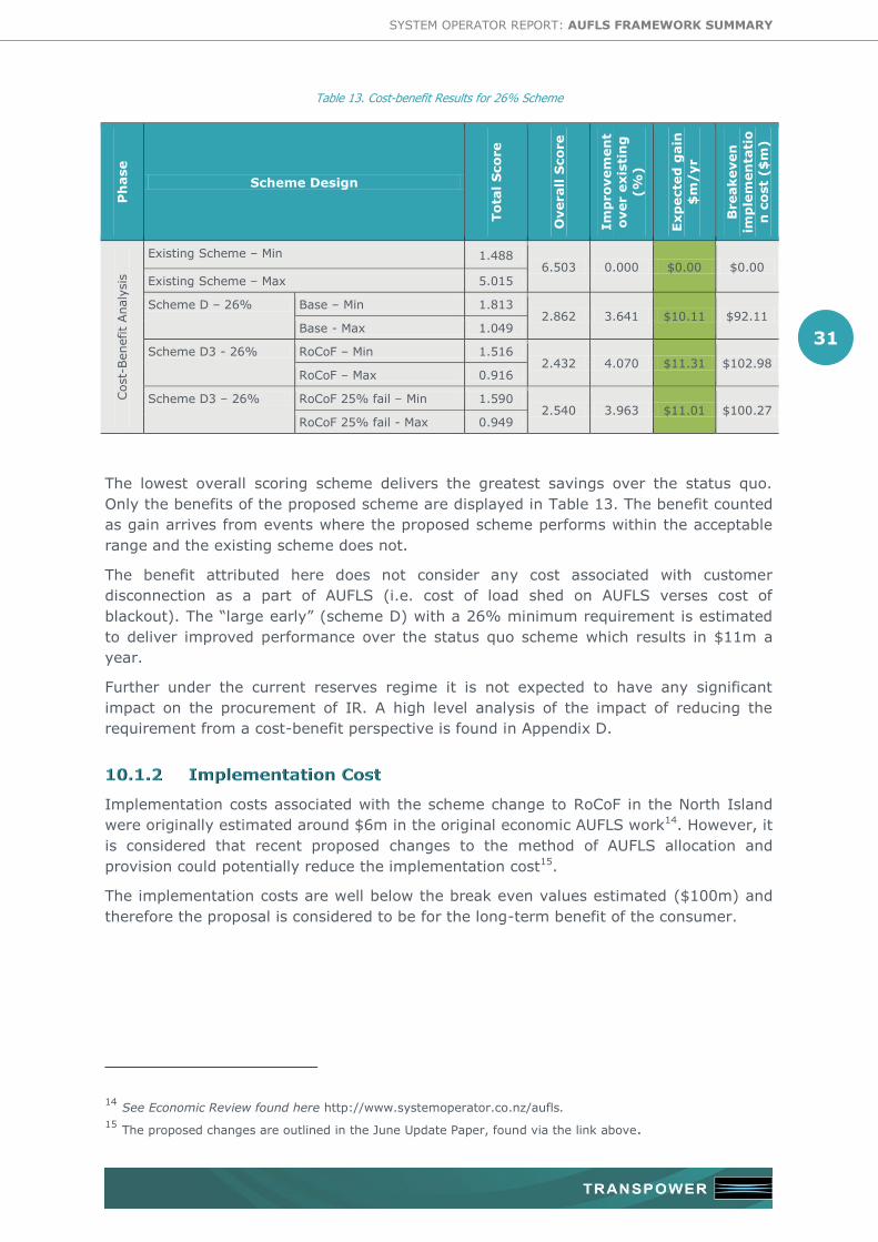
SYSTEM OPERATOR REPORT: AUFLS FRAMEWORK SUMMARY
31
Table 13. Cost-benefit Results for 26% Scheme
Ph
ase
Scheme Design
To
tal S
co
re
Overall S
co
re
Im
pro
vem
en
t
over e
xis
tin
g
(%
)
Exp
ecte
d g
ain
$m
/yr
Breakeven
imp
lem
en
tati
o
n c
ost
($
m)
Cost-
Benefit
Analy
sis
Existing Scheme – Min 1.488 6.503 0.000 $0.00 $0.00
Existing Scheme – Max 5.015
Scheme D – 26% Base – Min 1.813 2.862 3.641 $10.11 $92.11
Base - Max 1.049
Scheme D3 - 26% RoCoF – Min 1.516 2.432 4.070 $11.31 $102.98
RoCoF – Max 0.916
Scheme D3 – 26% RoCoF 25% fail – Min 1.590 2.540 3.963 $11.01 $100.27
RoCoF 25% fail - Max 0.949
The lowest overall scoring scheme delivers the greatest savings over the status quo.
Only the benefits of the proposed scheme are displayed in Table 13. The benefit counted
as gain arrives from events where the proposed scheme performs within the acceptable
range and the existing scheme does not.
The benefit attributed here does not consider any cost associated with customer
disconnection as a part of AUFLS (i.e. cost of load shed on AUFLS verses cost of
blackout). The “large early” (scheme D) with a 26% minimum requirement is estimated
to deliver improved performance over the status quo scheme which results in $11m a
year.
Further under the current reserves regime it is not expected to have any significant
impact on the procurement of IR. A high level analysis of the impact of reducing the
requirement from a cost-benefit perspective is found in Appendix D.
Implementation costs associated with the scheme change to RoCoF in the North Island
were originally estimated around $6m in the original economic AUFLS work14. However, it
is considered that recent proposed changes to the method of AUFLS allocation and
provision could potentially reduce the implementation cost15.
The implementation costs are well below the break even values estimated ($100m) and
therefore the proposal is considered to be for the long-term benefit of the consumer.
14 See Economic Review found here http://www.systemoperator.co.nz/aufls.
15 The proposed changes are outlined in the June Update Paper, found via the link above.
SYSTEM OPERATOR REPORT: AUFLS FRAMEWORK SUMMARY
32
11. SUMMARY OF FINDINGS AND RECOMMENDATIONS
The System Operator set out to determine a methodology to identify a reasonable level
of AUFLS coverage of the North Island power system. The “saw-tooth” methodology was
developed to provide a wider view of AUFLS performance and determine the reasonable
coverage level.
Allocating 32% demand to AUFLS provides a prudent coverage level
The results of the “saw-tooth” methodology indicated that within the current
limitations, and assuming static AUFLS provision, a 32% requirement provides a
prudent coverage level across the scenarios assessed.
A ‘large early’ four block scheme design provides effective coverage
The Four blocks made respectively of 10%, 10%, 6%, and 6% provided the
most effective coverage of the scheme designs considered.
AUFLS provision behaviour impacts the desired AUFLS requirement level
The expected provision range of AUFLS, specifically the amount of expected
surplus provision, will impact on the recommend AUFLS requirement level. The
outcomes of the Electricity Authority’s Extended Reserves Procurement project
will shape the structure and level of the AUFLS Requirement.
Reducing the requirement may be necessary to manage surplus
provision
If the practice of surplus AUFLS allocation is expected to continue after any
future procurement method changes then the System Operator may recommend
reducing the minimum requirement to 26% and adjusting the scheme design to
four blocks made of 8%, 8%, 5%, and 5% respectively.
An incremental approach to the use and settings of RoCoF relays is
recommended
The use of RoCoF relays adds benefit to the scheme design but to minimise risk
associated with the unproven technology it was recommended that only the
fourth block be armed of the strongest performing under-frequency scheme.
The analysis identified that future performance improvements could be made
once greater confidence is the use of RoCoF relays is gained. Further
improvements can be made from reducing the operating time of the AUFLS relay
to circuit breaker configurations.
Future investigation should be given to the use of over-frequency
reserves in relation to AUFLS
The analysis demonstrated that within the current design limitations all of the
schemes assessed result in some level of over-shedding and over-frequency
risk. The use of over-frequency reserves, particularly during the day, could be
used to improve system reliability. However further investigation is required and
will be carried out as a part of the UFM project.
The aim of the investigation was to identify an improvement from the status quo that is
implementable in the near future. The large early (10%, 10%, 6%, and 6%) scheme
proposed provides greater reliability than the current AUFLS scheme and is
recommended that the change to the proposed scheme design are made as soon as
practicable.

SYSTEM OPERATOR REPORT: AUFLS FRAMEWORK SUMMARY
33
12. LINKS TO ADDITIONAL INFORMATION
If you would like further background information on these various under-frequency
management and AUFLS initiatives, the following web links are likely to be useful:
http://www.systemoperator.co.nz/aufls. This web-page details the various
elements of the System Operator’s investigations into the performance of
existing and potential new AUFLS arrangements.
http://www.systemoperator.co.nz/f5573,84053156/20130630_AUFLS_u
pdate_Jun_2013.pdf. This links to the June Update paper which includes
proposal to improve AUFLS provision behaviour and compliance
practices.
http://www.systemoperator.co.nz/f5573,75968707/Automatic-under-
frequency-load-shedding-RoCoF-testing-summary-web.pdf This links to
the RoCoF Bench Testing Report completed in 2012.
http://www.systemoperator.co.nz/ufm . This web page provides detailed
information about the broader Under-Frequency Management (UFM) project
http://www.ea.govt.nz/our-work/programmes/pso-cq/under-frequency-
management/aufls/. This web page provides more information about the issues
associated with the AUFLS exemptions, and the Authority’s proposed approach
to addressing the issues identified.
http://www.ea.govt.nz/our-work/consultations/pso-cq/efficient-procurement-
extended-reserves/. This web page contains the consultation papers published
by the Electricity Authority on different procurement methods for AUFLS load.

SYSTEM OPERATOR REPORT: AUFLS FRAMEWORK SUMMARY
34
13. APPENDIX A: PROBABILITY DISTRIBUTION
METHODOLOGY
The purpose of this appendix is to outline the methodology used to create the probability
distribution function for each event analysed in the saw-tooth methodology.
Data from 10-Apr-2010 until 10-Apr-2013 was collected at half hourly intervals. At each
time-step, the inertia from all the running machines were summed to calculate the
system inertia. From the calculated system inertia the expected df/dt following an event
can be calculated. For example, the expected df/dt from the loss of Huntly station or the
loss of the HVDC was calculated using the formula
( )
Where
denotes the change in frequency in Hz/s, denotes the inertia in MWs, and
denotes the power in MW. The HVDC is assumed to be running in the Huntly station trip
case, and it is assumed to share the frequency perfectly between the North and South
Islands, so the system inertia is the sum of the inertia of both islands. The total NZ
inertia was chosen instead of the North Island inertia when the HVDC is out of service,
since the data is from the last 3 years where Pole 1 has not been used as often. With
Pole 3 in-service, and especially when a national frequency market eventuates, it is more
likely in the future that at least one of the HVDC poles will be in service. For the HVDC
bipole trip, the HVDC is out of service, and thus only the inertia of the North Island
generators is relevant (for a North Island event).
Using a selection of frequency events from 2009 to 2012, the initial system df/dt
measured from Phasor Measurement Units (PMUs) was compared to the expected df/dt
calculated using the method, described above. The results are shown to match relatively
well as shown in Figure 7.
Figure 7: Expected vs measured df/dt for a range of events.
Based on the historic data, the cumulative percentage and probability distribution
function (pdf) of the df/dt for a Huntly station trip and a HVDC bipole trip were calculated
-0.8 -0.6 -0.4 -0.2 0 0.2 0.4 0.6-0.8
-0.6
-0.4
-0.2
0
0.2
0.4
0.6
(Gen Loss) --- Measured df/dt (Hz/s) --- (Load Loss)
Expecte
d d
f/dt
(Hz/s
)

SYSTEM OPERATOR REPORT: AUFLS FRAMEWORK SUMMARY
35
as shown in Figure 8. Historically the Huntly event has been more severe, but
progressive decommissioning of Huntly generation units and commissioning of Pole 3 is
expected to close or even reverse the gap.
Figure 8: (a) Cumulative percentile and (b) pdf of expected df/dt for a Huntly station trip, an HVDC bipole trip, and a Huntly station trip with the HVDC out of service.
For each TSAT-simulated event, the initial df/dt is calculated and plotted versus the MW
tripped as shown in Figure 9a. Since AUFLS occurs well after the initial df/dt, the df/dt to
MW trip curve is the same regardless of AUFLS scheme used. A quadratic fit through the
origin is then used to smooth the graph, since energy is proportional to , so the power
deficit, or the change in energy over time, is proportional to
.
The quadratic is then used to map df/dt to MW for the historic df/dt data to give the pdf
of MW trip size as shown in Figure 9b. The TSAT simulation can then be thought of as
calculating the expected AUFLS performance over a section of the pdf. The section of the
pdf observed is dependent upon the system snapshot simulated in TSAT. A plot of the
observed regions of the pdf for the five TSAT cases is shown in Figure 10.
A minimum pdf level of 0.05% every 10 MW is applied to cover for high impact low
probability events not captured in the pdf. This “black swan” factor allows schemes which
have better performance with high df/dt events such as a bipole trip with sympathetic
generation trip) to be distinguished.
Figure 9: (a) Calculated df/dt from simulation vs MW tripped with quadratic smoothing (b) pdf vs MW trip showing the observed range and modified pdf
-2.5 -2 -1.5 -1 -0.5 0 0.5 10
10
20
30
40
50
60
70
80
90
100
Expected df/dt (Hz/s)
Cum
ula
tive P
erc
entile
HLY Trip
HVDC Trip
HLY Trip with HVDC out
-2 -1.8 -1.6 -1.4 -1.2 -1 -0.8 -0.6 -0.4 -0.20
0.2
0.4
0.6
0.8
1
1.2
1.4
1.6
1.8
2
Expected df/dt (Hz/s)
Pro
babili
ty D
istr
ibution F
unction
HLY Trip
HVDC Trip
HLY Trip with HVDC out
0 200 400 600 800 1000-1.4
-1.2
-1
-0.8
-0.6
-0.4
-0.2
0
MW Trip
df/
dt
(Hz/s
)
Calculated df/dt from simulation
Quadratic smoothed df/dt
MW Trip (MW)
Pro
babili
ty D
istr
ibution F
unction (
%)
0 200 400 600 800 1000 12000
0.05
0.1
0.15
0.2
0.25
Observed range
Original pdf
With lower limit

SYSTEM OPERATOR REPORT: AUFLS FRAMEWORK SUMMARY
36
Figure 10: Coverage of the simulations on the expected df/dt pdfs.
-2 -1.8 -1.6 -1.4 -1.2 -1 -0.8 -0.6 -0.4 -0.20
0.5
1
1.5
2
Expected df/dt (Hz/s)
Pro
babili
ty D
istr
ibution F
unction
Light load, HVDC out, HLY trip
Med load, HLY trip
Med load, HVDC out
High load, HLY out
High load, HVDC outHLY Trip
HVDC Trip
HLY Trip with HVDC out

SYSTEM OPERATOR REPORT: AUFLS FRAMEWORK SUMMARY
37
14. APPENDIX B: OPERATING TIME
Technical analysis has shown that minimising the operating time of AUFLS relay
arrangements has a benefit to the overall effectiveness of the scheme. A review of the
AUFLS system as it stands has highlighted that there is scope to ‘speed-up’ the operating
times of many relay arrangements simply by minimising ‘introduced’ time delays.
Sensing frequency events and disconnecting demand primarily involves an arrangement
of protection relays, tripping relays, and circuit breakers. The components that make up
the total operating time of any protection scheme is shown in Figure 11.
Figure 11 - Protection scheme operating time components
Protection relays have a specific ‘sensing time’ (A-B) which is usually fixed and cannot be
adjusted. Most arrangements also include one or more adjustable time delays (B-C)
which may either be built into the protection relay and/or are provided by separate time
delay relays. The adjustable time delays in AUFLS relay arrangements are used to ensure
the frequency stays at or below a trigger point for a specified amount of time. The
adjustable delays are also used to provide the different time delays presently specified
for AUFLS blocks 1 and 2.
Most arrangements feature a separate ‘tripping relay’ which has a finite and usually non-
adjustable operating time (C-D). The circuit breaker also has a finite operating time
measured from when it receives a ‘trip’ signal to when the primary contacts separate (D-
E). The table below provides some context as to the typical ranges of the above ‘fixed’
times:
Protection relay sensing time (usually fixed)
Tripping relay operating time (fixed)
Circuit breaker operating time (fixed)
Freq
uen
cyFr
equ
ency
Time
Operating time (excluding CB arcing time)
Adjustable time delay
B
C
A
D
E

SYSTEM OPERATOR REPORT: AUFLS FRAMEWORK SUMMARY
38
Table 14 Time Delays for a typical relay arrangement
Item Typical time
Protection relay sensing time (A-B) 100 ms
Tripping relay operating time (C-D) 20 ms
Circuit breaker operating time (D-E) 40 ms16
Total ‘fixed’ time delay 160 ms
The System Operator is proposing the total ‘operating time’ for all AUFLS relay
arrangements blocks be kept as short as practicable while still allowing for sufficient time
to prevent spurious tripping during transient frequency dips.
It is proposed that the only ‘introduced’ time delay is 100ms provided between the
protection relay having sensed a frequency drop (point B) and a ‘trip’ signal being
propagated to the tripping relay (point C). This will result in a total operating time of
around 250ms for most typical AUFLS relay arrangements without having to alter the
400ms maximum operating time presently specified in The Code17.
The testing requirements for AUFLS schemes will include measuring the time delay
between the frequency falling below the tripping threshold (point A) and the propagation
of a signal to the tripping relay (point C) as well ensuring the ‘adjustable’ time delay
(B-C) is set to 100ms. The requirements will also specify that no other adjustable time
delays be introduced apart from B-C above.
16 This is typical for most modern types of circuit breaker. Some older circuit breakers can be significantly
slower than this.
17 The Code presently sets out that the distributor must disconnect demand within 400ms after the frequency
reduces to, and remains at or below, the AUFLS trigger point. 400ms is the ‘maximum’ operating time however
this in some cases this appears to have been treated as a ‘target’.

SYSTEM OPERATOR REPORT: AUFLS FRAMEWORK SUMMARY
39
15. APPENDIX C: USE OF RATE OF CHANGE OF
FREQUENCY (ROCOF) RELAYS
A large loss of generation will almost always result in a correspondingly rapid rate of
change in frequency. It follows therefore that detecting df/dt and using it to trip AULFS
load is likely to be beneficial in an AUFLS scheme. This may be particularly useful when
there is a small frequency band within which AUFLS is required to operate such as in the
North Island
Many manufacturers offer relays with RoCoF functionality, but they are often intended to
be used for anti-islanding protection where rates of frequency change tend to be large
and are easily distinguished from ‘normal’ frequency excursions.
The type of frequency excursion that may trigger AUFLS relays vary from those that
have relatively low rates of frequency change, to those with very rapid rates of change.
In addition, there is usually some sort of disturbance on the system that has caused the
event and which will introduce ‘noise’ or distorted frequency traces. It is the noise in
particular that is of concern when RoCoF relays are being considered for use with AUFLS.
Bench testing of a selection of relays fitted with RoCoF functionality18 found that errors
can appear during the calculation of RoCoF, especially during system transients and
under unusual system conditions. These errors may result in either the RoCoF operating
when it shouldn’t, or it failing to operate when it should. A conservative implementation
of RoCoF is therefore recommended as a first step in order to limit its impact should an
error occur.
SETTINGS 15.1
Analysis of actual and simulated losses of generation shows that the fall of frequency is
greatest just after the event. As the event progresses, the rate of change in frequency
decreases as mechanisms such as interruptible load and AUFLS relays operate.
The analysis shows that for the use of RoCoF to have maximum effect, the block armed
with RoCoF should operate before the frequency and time blocks, when the rate of
change is steeper. The details of the settings and arrangement of RoCoF are based on
this premise.
18 Refer to RoCoF testing report found at http://www.systemoperator.co.nz/f5573,75968707/Automatic-under-
frequency-load-shedding-RoCoF-testing-summary-web.pdf

SYSTEM OPERATOR REPORT: AUFLS FRAMEWORK SUMMARY
40
The magnitude of the df/dt setting must be set high enough19 that it will not trip for
contingent events (CE’s). The maximum predicted initial df/dt from CE’s is shown in
Figure 12a. The CCGT plot refers to the maximum expected df/dt from the loss of
HLY-U5, OTC or SPL. The magnitude of initial df/dt from a single CE does not usually
exceed 0.8 Hz/s.
Figure 12: (a) Expected df/dt for a CE event, (b) expected df/dt from two simultaneous CE events.
During commissioning of large items of plant, such as a large generating unit, additional
reserves are procured such that the frequency will not fall below 48 Hz for a loss of CE
and a secondary trip of the asset being commissioning. To estimate the worst case, the
maximum expected df/dt from the loss of two CE was analysed from historical data and
is shown Figure 12b. These curves represent the worst case expected initial df/dt at the
point in time of two simultaneous CE’s (normally Pole 2 and a large CCGT) as they are
based on the historic conditions where no additional reserves were procured.
The initial df/dt for two simultaneous CE’s rarely goes above 1.3 Hz/s. For added
confidence, the RoCoF settings are set to not operate until the frequency has reached
48.5 Hz, this is known as the frequency guard and is covered in more detail in the next
section. Allowing for additional reserves and the reduction in the system df/dt by the
time the frequency is at 48.5 Hz, the RoCoF AUFLS block would be unlikely to trip for
most secondary trips during commissioning20.
Further for the commissioning of significantly sized units assessments can be completed
to ensure the df/dt will not result in RoCoF blocks tripping and planning work can be
completed to avoid high injection commissioning test occurring during very light load
(when the inertia is low).
The RoCoF setting must be set low enough that it will trip during severe ECE’s. A
histogram of the expected df/dt is shown in Figure 8 in Appendix A, where a setting of
1.2 Hz/s can be seen to be useful for the most severe ECE’s considered, with additional
benefits for even larger “black swan” events.
19 For the purpose of AUFLS, the rate of frequency fall or negative df/dt is of concern; this section will refer to
the magnitude of the setting in terms of a positive value for simplicity. 20 The timing of the secondary event impacts the overall size of risk that can be discriminated.
-1 -0.8 -0.6 -0.4 -0.2 00
500
1000
1500
Worst case df/dt from a CE (Hz/s)
Count
Pole 2
CCGT
Combined
-2 -1.5 -1 -0.5 00
500
1000
1500
Worst case df/dt from two CEs (Hz/s)
Count
Pole 2 + CCGT
2 CCGT
Worst Case

SYSTEM OPERATOR REPORT: AUFLS FRAMEWORK SUMMARY
41
A RoCoF setting of 1.2 Hz/s therefore is recommended as it is sufficiently removed from
the maximum expected df/dt of 0.8 Hz/s for a CE to allow for the possible loss of
accuracy that has been observed during bench testing, while still being in the range
where it can provide additional protection against large system disturbances.
Figure 13: (a) Expected df/dt for a CE event, (b) expected df/dt from two simultaneous CE events.
To guard against the possibility of RoCoF tripping when it shouldn’t, a time delay will be
applied to the RoCoF element, such that the measured df/dt will have to be greater than
the setting for a pre-set length of time before the relay can trip. This will cause the relay
to err on the side of not-tripping. The delay is of most benefit with noisy frequency
signals that can result in large calculated df/dt but it will also help reduce the df/dt error
caused by sinusoidal power oscillations.
During system events, there is likely to be noise in the frequency measurements. This
noise can be in the form of short transients, or power oscillations from rotor angle
swinging. A small amount of high frequency noise is sufficient to greatly increase the
noise in the df/dt.
A delay filter of at least 100ms will be applied, so the measured df/dt will have to be
above the set point for at least 100ms before the relay will trip. This is likely to be
extremely helpful in eliminating the noise caused by short transients, but problems may
still exist with power oscillations.
The delay window will have an effective “bode plot” in that it will increase the magnitude
of the power oscillation required to trip the relay. For example, a power oscillation of >5
Hz will have a half cycle of 100ms. Since any half cycle will go through zero, power
oscillations of >5 Hz will be completely eliminated by the 100ms delay filter.
The bode plot of the filter responses with and without a 100ms delay is shown in Figure
14. The delay filter is seen to significantly improve the bode plots by providing filtering at
higher frequencies.
-1 -0.8 -0.6 -0.4 -0.2 00
500
1000
1500
Worst case df/dt from a CE (Hz/s)
Count
Pole 2
CCGT
Combined
-2 -1.5 -1 -0.5 00
500
1000
1500
Worst case df/dt from two CEs (Hz/s)
Count
Pole 2 + CCGT
2 CCGT
Worst Case

SYSTEM OPERATOR REPORT: AUFLS FRAMEWORK SUMMARY
42
Figure 14: (a) Bode plot with no delay, (b) Bode plot with 100ms delay
The df/dt error caused by an oscillation of 2° peak to peak amplitude is shown in Figure
15. The delay window can be seen to significantly improve performance.
Figure 15: (a) df/dt error with oscillation of fixed size, (b) df/dt error with oscillation of fixed size
All of the relays provide reasonable resistance to noise when combined with the 100ms
delay, especially since the guard frequency provides significant additional protection.
Relays with heavier filtering such as the GE760 may be more suitable if all other factors
are equal, but cost, ease of use and integration into existing systems should be the
primary determinants of relay choice21.
A guard frequency setting will be applied to the df/dt element to prevent it from tripping
when the frequency is above 48.5 Hz. This will ‘lock-out’ the df/dt element for most
normal frequency excursions, while still providing enough headroom for it to be effective
during large frequency excursions.
A logic diagram of the required df/dt tripping logic is shown below22.
21 Note also that staying connected during noisy events which lower the frequency may have unexpected
effects on equipment, so staying connected is not necessarily always better. 22 Note the df/dt element value is described in terms of magnitude here, in practice the df/dt setting is (df/dt <
-1.2 Hz).
0 1 2 3 4 5 6 70
0.1
0.2
0.3
0.4
0.5
0.6
0.7
0.8
0.9
1G
ain
Oscillation Frequency (Hz)
Bode plot with no delay window
SEL351 0.4Hz/s
SEL351 1.5Hz/s
GE760 0.4Hz/s
GE760 1.5Hz/s
P145 0.96s
P145 0.2s
7SJ64 0.4Hz/s
7SJ64 1.5Hz/s
7SJ80 0.4Hz/s
7SJ80 1.5Hz/s
0 1 2 3 4 5 6 70
0.1
0.2
0.3
0.4
0.5
0.6
0.7
0.8
0.9
1
Gain
Oscillation Frequency (Hz)
Bode plot with 0.1s delay window
SEL351 0.4Hz/s
SEL351 1.5Hz/s
GE760 0.4Hz/s
GE760 1.5Hz/s
P145 0.96s
P145 0.2s
7SJ64 0.4Hz/s
7SJ64 1.5Hz/s
7SJ80 0.4Hz/s
7SJ80 1.5Hz/s
0 1 2 3 4 5 6 70
0.1
0.2
0.3
0.4
0.5
0.6
0.7
0.8
0.9
1
dfd
t err
or
(Hz/s
)
Oscillation Frequency (Hz)
df/dt for a 2 deg pk-pk phase oscillation with no delay window
SEL351 0.4Hz/s
SEL351 1.5Hz/s
GE760 0.4Hz/s
GE760 1.5Hz/s
P145 0.96s
P145 0.2s
7SJ64 0.4Hz/s
7SJ64 1.5Hz/s
7SJ80 0.4Hz/s
7SJ80 1.5Hz/s
0 1 2 3 4 5 6 70
0.1
0.2
0.3
0.4
0.5
0.6
0.7
0.8
0.9
1
dfd
t err
or
(Hz/s
)
Oscillation Frequency (Hz)
df/dt for a 2 deg pk-pk phase oscillation with 0.1s delay window
SEL351 0.4Hz/s
SEL351 1.5Hz/s
GE760 0.4Hz/s
GE760 1.5Hz/s
P145 0.96s
P145 0.2s
7SJ64 0.4Hz/s
7SJ64 1.5Hz/s
7SJ80 0.4Hz/s
7SJ80 1.5Hz/s
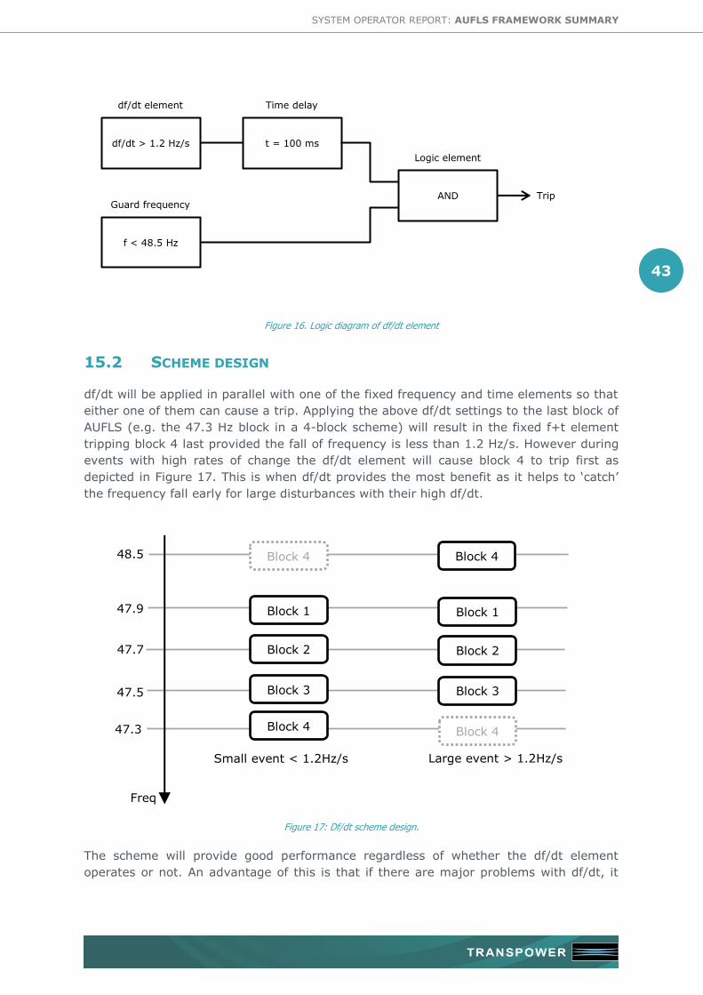
SYSTEM OPERATOR REPORT: AUFLS FRAMEWORK SUMMARY
43
Figure 16. Logic diagram of df/dt element
SCHEME DESIGN 15.2
df/dt will be applied in parallel with one of the fixed frequency and time elements so that
either one of them can cause a trip. Applying the above df/dt settings to the last block of
AUFLS (e.g. the 47.3 Hz block in a 4-block scheme) will result in the fixed f+t element
tripping block 4 last provided the fall of frequency is less than 1.2 Hz/s. However during
events with high rates of change the df/dt element will cause block 4 to trip first as
depicted in Figure 17. This is when df/dt provides the most benefit as it helps to ‘catch’
the frequency fall early for large disturbances with their high df/dt.
Figure 17: Df/dt scheme design.
The scheme will provide good performance regardless of whether the df/dt element
operates or not. An advantage of this is that if there are major problems with df/dt, it
df/dt > 1.2 Hz/s
df/dt element
f < 48.5 Hz
Guard frequency
t = 100 ms
Time delay
AND
Logic element
Trip
Block 1
Block 2
Block 3
Block 4
Block 1
Block 2
Block 3
Block 4
48.5
47.9
47.7
47.5
47.3
Freq
Small event < 1.2Hz/s Large event > 1.2Hz/s
Block 4
Block 4

SYSTEM OPERATOR REPORT: AUFLS FRAMEWORK SUMMARY
44
can be turned off and AUFLS will continue to perform well as a four block f+t only
scheme.
The overall tripping logic for the df/dt plus f+t AUFLS block is shown below.
Figure 18: Logic diagram of df/dt with fixed f+t element.
Relays that cannot accommodate this arrangement of logic will be precluded from being
used in the scheme.
OTHER FEATURES 15.3
There are some additional features that are desirable in a scheme that features df/dt.
These features are not essential but they would be useful in allowing the performance of
the scheme to be more easily monitored.
The initial implementation of df/dt as described above is intended to allow the System
Operator to realise the benefits of it without placing the AUFLS system at high risk
should it fail to operate as expected.
Accordingly, it would be desirable to have a feature that allows for the df/dt elements to
be easily disabled (switched off) should this be desired for any reason.
This feature would ideally allow for the df/dt element to be disabled by an operator via a
local switch / pushbutton or via a SCADA control rather than via technician having to
interface a computer to the relay.
The ability to identify whether the df/dt element of an AUFLS relay had operated during a
frequency event is important as it will aid with post event analysis. The flagging of
df/dt < -1.2 Hz/s
df/dt element
f < 48.5 Hz
Guard frequency
t = 100 ms
Time delay
AND
Logic element
Trip
f < 47.3 Hz
Fixed frequency
OR
Logic element
t = 100 ms
Time delay

SYSTEM OPERATOR REPORT: AUFLS FRAMEWORK SUMMARY
45
operation would preferably be via SCADA as local flagging would necessitate visits to all
sites where df/dt relays were in service.
Event capture is a feature of some relays that allows system parameters (e.g. voltage
and frequency) to be recorded before, during and after an event. Having this type of
information would also aid in post event analysis.
SPECIFICATION AND PERFORMANCE REQUIREMENTS 15.4
The df/dt relay settings and list of desirable features form the basis of a technical
specification for AUFLS df/dt relays. The specification is as follows:
Feature Required Notes
Df/dt element:
Number of elements 1
Range of settings -1.0 to -2.0 Hz/s
Resolution of settings 0.1 Hz/s
Adjustable time delay 0 to 500ms
Fixed frequency element:
Number of elements 2
Range of settings 50 to 47 Hz
Resolution of settings 0.1 Hz
Adjustable time delay 0 to 500ms
Other requirements:
Customisable logic As per Figure 16
Feature Details
Remote enable/disable of df/dt element Via SCADA or via front panel
Flagging of df/dt operation Via SCADA or via front panel
Event logging
In addition, the following information is required for any df/dt relay proposed for use on
the AUFLS system:
Manufacturer and model
Stated accuracy
Stated repeatability
List of standards which it complies with (e.g. EMI withstand etc.)
Available communication interfaces

SYSTEM OPERATOR REPORT: AUFLS FRAMEWORK SUMMARY
46
Transpower has independently tested a number of readily available df/dt relays in order
to understand how they respond to simulated under frequency events. This information
has helped us form a view as to how df/dt is likely to perform in service.
Transpower’s aim is not to determine which relays should be used by industry but to
identify the needed performance requirements. Transpower has the required equipment
and files available should a group wish to test a relay not covered in the bench testing
analysis.

SYSTEM OPERATOR REPORT: AUFLS FRAMEWORK SUMMARY
47
16. APPENDIX D: AUFLS REQUIREMENT CHANGES
COST BENEFIT ANALYSIS
PURPOSE 16.1
As part of the technical work the System Operator considered the impact of changing the
amount of pre-event demand allocated to Automatic Under-Frequency Load Shedding
(AUFLS) in the North Island. The amount of pre-event demand allocated to AUFLS is
known as the AUFLS requirement. The System Operator approached the Electricity
Authority and Concept Consulting to assist in identifying the key cost and benefit
categories that would be impacted by changing the AUFLS requirement or scheme design
(i.e. number, relative size, and trip settings of the different blocks).
This report outlines the high level analysis of how the cost and benefit categories change
in relation to future state of the system and the AUFLS Requirement.
The AUFLS Requirement is the level of pre-event system demand, generally referred to
as a percentage of island load, allocated for AUFLS. The overall performance and cost of
AUFLS is impacted both by the requirement and how the load is allocated, organized and
triggered, i.e. the scheme design.
Different scheme designs can have markedly different costs and benefits, even though
they may have the same percentage of load under AUFLS. The number of load blocks,
and the tripping mechanism, play a significant role in determining many of the costs
which make up the overall cost of a scheme.
In addition to system security performance, there are a number of other considerations
which can influence the ‘optimal’ size of the AUFLS Requirement. For example, as set out
later in this Appendix, increases in the instantaneous reserve costs is a critical factor in
considering reducing the AUFLS requirement. Conversely, if the AUFLS requirement
increases, AUFLS impacts on reserve costs would fall to zero and the dominant costs
would arise from the scheme’s load shedding efficiency (disconnecting AUFLS blocks
when needed), and over frequency collapse costs arising from over-shedding of AUFLS
load.
The principal focus of the high-level Concept analysis was in relation to the non-system
collapse costs associated with different AUFLS requirements. This is because the System
Operator was undertaking the analysis necessary to evaluate the likely nature and scale
of variation in under- and over-frequency system collapse costs with different scheme
designs.
This appendix sets out the key conclusions of the Concept analysis relating to:
IR costs
AUFLS load shedding costs
AUFLS relay costs
Over-frequency arming
The report is based on work completed by Simon Coates of Concept Consulting and the
System Operator would like to thank him for his contribution.

SYSTEM OPERATOR REPORT: AUFLS FRAMEWORK SUMMARY
48
INSTANTANEOUS RESERVE PROCUREMENT COST 16.2
Reserves and energy are similar products but are used for different purposes and offered
at different prices. Reserves can be seen as dedicated capacity, or energy on standby,
available when the system conditions require it in the event of the sudden loss of net
injection. Many generators can offer capability as either energy or reserve, or a
combination of the two. Instantaneous Reserves (IR) are procured to cover both the
contingent event (CE) and extended contingent event (ECE) risk on the system. The
AUFLS scheme design is considered when calculating the amount of IR required to
sufficiently covering the ECE risk. Any changes to the AUFLS requirement could impact
the quantity of IR procured.
There are two main ways in which AUFLS arrangements can impact on IR costs:
1. Having insufficient AUFLS to cover the ECE, thereby giving rise to a need to
purchase increased quantities of IR above that necessary to cover the CE
2. Preventing load from being more valuably used to provide IR because it is instead
required to provide AUFLS.
The Concept analysis set out in this appendix only considered the implications of the first
factor. This is because the second factor is not an inherent feature in relation to the
AUFLS requirement, but is instead driven by the AUFLS procurement approach used to
acquire the load necessary to meet the AUFLS requirement. This procurement aspect is
the subject of a separate initiative being undertaken by the EA and SO, and was thus out
of scope for this exercise.
With respect to the first factor, the diagram below shows how having insufficient AUFLS
at any given moment in time could result in increased IR costs.
Figure 19 Illustration of how insufficient AUFLS may result in increased IR procurement
CE
ECE
IR
AUF
L
S
IR
Additional IR procured due to insufficient AUFLS available
Estimated AUFLS available from Requirement and Scheme Design
IR procured to cover CE

SYSTEM OPERATOR REPORT: AUFLS FRAMEWORK SUMMARY
49
The extent to which extra IR may be required for a given AUFLS Requirement will depend
on:
The size of the CE (and thus the amount of IR that would be procured anyway)
The size of the ECE
The amount of demand (and thus the amount of AUFLS that would be available
if the AUFLS requirement is specified as a percentage of demand)
All such factors exhibit considerable variation at different times of the day and year.
Accordingly, a framework was adopted which considered the likely implications of
different AUFLS requirements for different key time periods, distinguishing by season
(Summer, Shoulder, and Winter months) and time of day (Night, Day, and Peak).
A framework was also adopted which considered the two main drivers of IR costs:
The fixed costs of carrying extra capacity on the system to provide reserves;
and
The variable costs of making reserve available (principally the costs of running
some machines at lower efficiency to provide spinning reserve, or the costs of
running hydro machines in tail-water depressed mode)
The fixed carrying costs are effectively only incurred when capacity is scarce – i.e.
principally at times of peak demand, whereas the variable costs are incurred at all times
IR is required.
Figure 20 below illustrates this relationship. It also shows that the fixed carrying costs of
providing extra capacity on the system are orders of magnitude greater than the variable
costs of making IR available.
Figure 20. Historic relationship between IR prices and demand

SYSTEM OPERATOR REPORT: AUFLS FRAMEWORK SUMMARY
50
In terms of estimating the potential impact of different AUFLS requirements on IR costs,
the above analysis highlights that the principal potential cost impact would be if there
were insufficient AUFLS to cover the ECE at times of peak, as this would likely give rise
to an increased requirement to build generation capacity.
The marginal source of capacity at times of peak demand is assumed to be an open-cycle
gas turbine (OCGT) peaker. Even if such OCGTs are not directly used to provide IR,
building more OCGT peakers will free up other existing generation (e.g. hydro stations)
from providing energy to enable them to provide reserves. The carrying costs of a new
OCGT (i.e. annual fixed O&M costs, plus capital recovery costs) are assumed to be
$145,000/MW/yr. This is based on recent analysis undertaken by the Electricity
Authority in relation to capacity adequacy.
In comparison, the variable costs of IR provision are much less significant, estimated to
be of the order of $1-2/MW/h, based on inspection of historical IR offers.
Relatively simple analysis can be undertaken to estimate the ‘threshold’ AUFLS
requirement, below which it would be likely that there would be a need to procure more
IR at times of system peak.
Figure 21 Simple illustration of the steps required to estimate the threshold % AUFLS requirement at times of peak, below which there would be a need for extra IR to be procured
At the moment, the largest possible ECE is the loss of the HVDC bipole. Until recently,
the maximum northbound capacity of the HVDC bipole was 700MW. With the
commissioning of Pole 3 this has risen to 1,200MW (≈ 1,100 MW received i.e. after
losses across the HVDC), and in the future this could rise further to 1,400MW (≈1,300
MW received) if the capacity of the link is upgraded further.
At times of peak demand, the size of the CE is likely to be set by the largest CCGT in
operation. Generally, at times of winter peak demand, all the CCGTs are in operation.
However, it is possible that the largest, e3p, could be out of operation, so it could be that
the size of the CE is ‘only’ 365 MW, set by the Otahuhu B CCGT.
Peak North Island demand is approximately 4,400 MW.
Taking all of the above, and considering the situation of a 1,200 MW HVDC, it would
appear at first glance that the AUFLS requirement at peak would equal
1,100 MW – 365 MW = 735 MW ≈ 17% of peak demand.
And in a future where the HVDC capacity was increased to 1,400 MW, this requirement
would increase to ≈ 21%.
CE
ECE
IR
AUF
L
S
2. Subtract the smallest amount of IR that will be required to cover the CE at peak demand
1. Determine the size of maximum ECE that could be experienced at times of peak demand
3. The remaining amount is the AUFLS requirement. This can be expressed as a % of peak
demand.

SYSTEM OPERATOR REPORT: AUFLS FRAMEWORK SUMMARY
51
Based on this simplistic framework, an AUFLS requirement which was less than these %
values would appear likely result in the need to procure extra IR at peak.
However, this approach to considering the likely size of the ECE at times of peak
demand, ignores the fact that there may be insufficient ‘spare’ South Island generation
to send North after meeting South Island demand requirements at times of peak. Thus,
the HVDC may not be operating at full capacity at times of peak North Island demand.
Thus, at times of peak demand, it is likely that the balance of South Island generation
and demand will significantly limit the amount of transfer across the HVDC at times of
peak demand. Unless new South Island generation is built, then progressive growth in
South Island demand is likely to further reduce the size of northward HVDC transfer at
times of North Island peak demand.
The most significant factor that could change this is if the Tiwai smelter were to shut.
This would release an extra 600 MW of South Island generation which could be sent
north at times of system peak. This would mean that the HVDC could be at full capacity
at times of peak North Island demand.
Another factor that could potentially alter the IR requirements is if the definition of the
extended contingent event were to change. Two possible changes to the definition of the
ECE were identified which could increase the size of the ECE:
1. The addition of the largest single potential secondary plant trip to the ECE.
For example, adding the risk that the largest CCGT were to trip in response to
the under-frequency event caused by the original ECE trip. Such a secondary
trip would be in breach of the plant’s AOPOS and could thus be considered
unlikely23.
2. Classifying the loss of the largest potential site as an ECE. For example the
whole of the Huntly site (i.e. the original Huntly station, plus e3p, plus the P40
OCGT). Following the retirement of one of the Huntly station units, the
maximum size of the Huntly site is ≈ 1,185 MW. Again, the loss of a whole
23 Despite being unlikely, such a situation has occurred twice in the last decade.
SI Gen
Cap
SI Dem
Based on current SI peak gen and demand, the amount of ‘spare’ SI gen capacity is only ≈ 960 MW (890 MW received) which is ≈ 12% peak NI demand. This is less than the HVDC capacity. SI Generation
Capacity
Available generation to export to NI across HVDC
HVDC
SPARE

SYSTEM OPERATOR REPORT: AUFLS FRAMEWORK SUMMARY
52
site could be considered to be very unlikely, but certainly within the realms of
possibility with a return period of decades rather than years.
The next credible event review is next year. It is possible, although unlikely, that such a
review could result in a change in the ECE classification to include the type of additional
risk outlined above.
Accordingly, high-level analysis was undertaken which considered all these different
possible changes in physical risk and credible event classification, and calculated the
consequent size of the ECE minus the CE and expressed it as a percentage of peak NI
demand – i.e. the ‘threshold’ AUFLS requirement at peak, below which an increase in IR
costs could be expected to occur. This is shown in the following figure:

SYSTEM OPERATOR REPORT: AUFLS FRAMEWORK SUMMARY
53
Figure 22. Estimate of the impact of difference physical system states, and credible event definitions, on the 'threshold' peak AUFLS requirement, below which significant increase in IR cost would be likely to occur

SYSTEM OPERATOR REPORT: AUFLS FRAMEWORK SUMMARY
54
As can be seen, if the ECE definition does not change (corresponding with the ECE =
HVDC and 0MW 2ndry risk categories in the graph), then the threshold peak AUFLS
requirement is at very low levels (10-14% or 17-20%, depending on whether Tiwai
continues to be in, or is out).
However, if the ECE definition were to change next year to include both a secondary trip
risk and the Huntly site, then AUFLS requirements of 30% or less at peak could start to
have material IR impacts.
In this respect it is worth noting that it would likely not be cost-effective to procure
additional reserves at times of peak to cover such extremely low probability events.
However, it could be cost-effective to procure AUFLS – i.e. setting the requirement at a
large enough level to cover such events – provided the increased costs of AUFLS load
shedding and over-frequency collapse risk do not outweigh the benefit from increased
security.
The System Operator has undertaken such analysis for the purpose of determining the
appropriate AUFLS requirement, through considering the probability distribution function
of different sized events for different system states. Given the above, it is considered
unlikely that the ECE definitions will change to include the risk of secondary trip risks
and/or whole-of-site loss risks.
It is worth noting that this ‘threshold’ AUFLS requirement will be significantly less at off-
peak times due to the fact that there will be significant ‘spare’ capacity available to
provide extra IR if required. Simple analysis suggests that the threshold requirement is
likely to be of the order of 8% less for ‘day’ periods, and approximately 25% less for
night periods.
For example, if the physical system state, and contingent event definition were such that
the ‘threshold’ AUFLS requirement at times of peak demand was 27%, then the
threshold requirement during day periods would be 27% - 8% = 19%, and for night
periods it would be 27% - 25% = 2%.
This is an important conclusion, because it suggests that the IR cost impact of different
requirements could be very different for different times of the day and year.
In terms of estimating the potential scale of cost impact, for every 1% the requirement
is set below the ‘threshold’ peak AUFLS requirement, the increased system capacity costs
are likely to be of the order of $6m per year.
AUFLS LOAD SHEDDING COSTS 16.3
Every time load is shed during an AUFLS event, those customers who are beneath the
AUFLS feeder will incur an interruption costs. With estimates of the value of lost load
(VoLL) for different customers ranging between $10,000 to $30,000/MWh (and more in
some cases), these costs can be significant.
As the AUFLS requirement increases, the amount of load which will be shed during an
AUFLS event will also increase.
Accordingly, analysis was undertaken to understand the potential scale of AUFLS load
shedding costs, and how such costs may vary with different AUFLS quantity
requirements and scheme design (i.e. the number and relative size of the different
blocks).
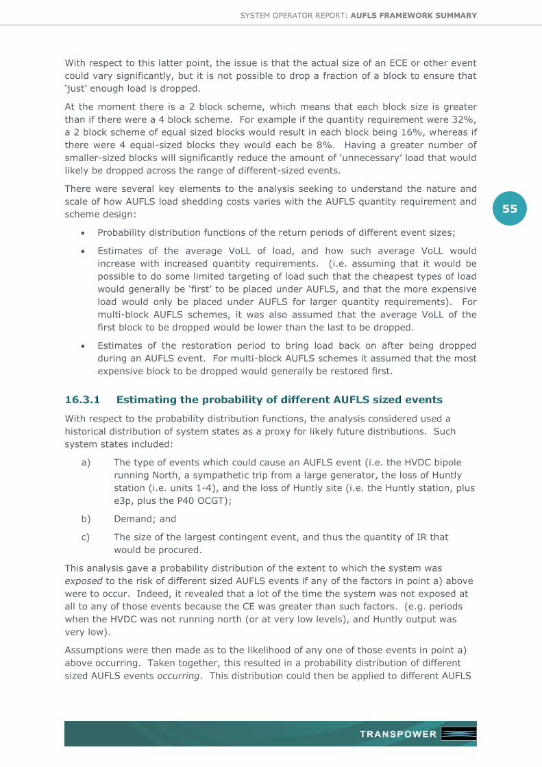
SYSTEM OPERATOR REPORT: AUFLS FRAMEWORK SUMMARY
55
With respect to this latter point, the issue is that the actual size of an ECE or other event
could vary significantly, but it is not possible to drop a fraction of a block to ensure that
‘just’ enough load is dropped.
At the moment there is a 2 block scheme, which means that each block size is greater
than if there were a 4 block scheme. For example if the quantity requirement were 32%,
a 2 block scheme of equal sized blocks would result in each block being 16%, whereas if
there were 4 equal-sized blocks they would each be 8%. Having a greater number of
smaller-sized blocks will significantly reduce the amount of ‘unnecessary’ load that would
likely be dropped across the range of different-sized events.
There were several key elements to the analysis seeking to understand the nature and
scale of how AUFLS load shedding costs varies with the AUFLS quantity requirement and
scheme design:
Probability distribution functions of the return periods of different event sizes;
Estimates of the average VoLL of load, and how such average VoLL would
increase with increased quantity requirements. (i.e. assuming that it would be
possible to do some limited targeting of load such that the cheapest types of load
would generally be ‘first’ to be placed under AUFLS, and that the more expensive
load would only be placed under AUFLS for larger quantity requirements). For
multi-block AUFLS schemes, it was also assumed that the average VoLL of the
first block to be dropped would be lower than the last to be dropped.
Estimates of the restoration period to bring load back on after being dropped
during an AUFLS event. For multi-block AUFLS schemes it assumed that the most
expensive block to be dropped would generally be restored first.
With respect to the probability distribution functions, the analysis considered used a
historical distribution of system states as a proxy for likely future distributions. Such
system states included:
a) The type of events which could cause an AUFLS event (i.e. the HVDC bipole
running North, a sympathetic trip from a large generator, the loss of Huntly
station (i.e. units 1-4), and the loss of Huntly site (i.e. the Huntly station, plus
e3p, plus the P40 OCGT);
b) Demand; and
c) The size of the largest contingent event, and thus the quantity of IR that
would be procured.
This analysis gave a probability distribution of the extent to which the system was
exposed to the risk of different sized AUFLS events if any of the factors in point a) above
were to occur. Indeed, it revealed that a lot of the time the system was not exposed at
all to any of those events because the CE was greater than such factors. (e.g. periods
when the HVDC was not running north (or at very low levels), and Huntly output was
very low).
Assumptions were then made as to the likelihood of any one of those events in point a)
above occurring. Taken together, this resulted in a probability distribution of different
sized AUFLS events occurring. This distribution could then be applied to different AUFLS

SYSTEM OPERATOR REPORT: AUFLS FRAMEWORK SUMMARY
56
quantity requirements and scheme designs to determine how much load would be
dropped, and thus the average AUFLS load shedding costs.
With respect to the likelihood of events occurring, the key return period assumptions
were:
• Failure of the HVDC bipole = 1 in 5 years (based on analysis in the last
credible event review)
• Failure of Huntly station = 1 in 9 years (based on the historical frequency of
occurrence of this event)
• Failure of the Huntly site = 1 in 30 years (guesstimate)
The risk of a secondary trip was considered to vary with the size of the primary event
relative to demand (and thus the speed at which system frequency was likely to fall).
Thus for a primary AUFLS event whose ECE minus CE size was equal to 2% of demand,
the risk of a secondary trip was considered to be 2%. However this grew to 20% for an
ECE-minus-CE event size equal to 60% of demand.
The historical data was also factored to take account of key system changes. In
particular:
• The HVDC capacity was scaled up to 1,200 MW northbound
• Huntly station was scaled down from 1,000 MW to 750 MW following the
recent mothballing of a unit
On balance, it was considered that this approach of scaling historical data would over-
estimate the likelihood of large scale risks occurring. This is because:
• Although the HVDC capacity has increased, the generation capability in the
South Island has not.
• Huntly station is likely to have a reduced generation capacity factor going
forward compared to that observed in the historical data set, due to factors
such as its continued displacement by new-build renewables.
However, it was considered appropriate to err on the side of over-estimating risks rather
than under-estimating. The probability distribution function that results from the
assumptions is displayed in Figure 23.

SYSTEM OPERATOR REPORT: AUFLS FRAMEWORK SUMMARY
57
The probability of the events requiring a significant amount of AUFLS (greater than 30%
demand) is low (considered being of the order of once every 100 years).
Figure 23 Probability distribution of likely AUFLS quantity required (expressed as a percentage of demand)

SYSTEM OPERATOR REPORT: AUFLS FRAMEWORK SUMMARY
58
The following graph show the estimated expected annual AUFLS load shedding cost for
the different quantity requirements and for different number of blocks24.
Such ‘expected’ annual numbers take account of the fact that AUFLS events are only
likely to occur once every five to six years or so.
As can be seen, as the AUFLS quantity requirement increases, a greater amount of load
will be shed for AUFLS events. However, having a larger number of smaller blocks better
enables ‘just’ enough load to be shed for a given sized event. For example, if the
requirement were set to 30% of load, then in a 1 block scheme that 30% of load would
be triggered even for relatively small AUFLS events (e.g. an event whose ECE minus CE
size was only equal to 5% of load). In a 4 block scheme, however, only the 1st block
would likely be triggered for such a small event.
This better ability to drop ‘just’ enough load accounts for the significantly lower AUFLS
load shedding costs for the 4 block scheme compared to the 1 and 2 block schemes.
The following two graphs display the above information but with the y-axis being
expressed in the first graph as the average $/MW/h cost of AUFLS load shedding, and in
the second graph as the incremental $/MW/h cost of AUFLS load shedding. Again,
expressing such costs on a per hour basis takes account of the fact that AUFLS events
are only likely to happen once every five to six years or so, and for multi-block schemes
the return period of the last block being triggered could be an order of magnitude less
likely than the first block being triggered.
24 The load shedding analysis assumed equal size for the 2 block scheme, but an 8:8:5:5 proportion for the 4
block scheme.
Figure 24. Estimated annual AUFLS load shedding costs for different requirements and blocks

SYSTEM OPERATOR REPORT: AUFLS FRAMEWORK SUMMARY
59
Figure 25. Average and incremental cost of AUFLS requirement and block number

SYSTEM OPERATOR REPORT: AUFLS FRAMEWORK SUMMARY
60
The above analysis demonstrates that:
• Having multiple blocks significantly reduced the average AUFLS load-shedding
cost
• For the purposes of analysis of the cost-benefit of different AUFLS quantity
requirements it would appear appropriate to assume for a four-block scheme
that the incremental AUFLS load-shedding cost for increased requirements
should be valued at approximately $0.25/MW/h.
Given that average NI demand is approximately 2,700 MW, this means that an increase
in the requirement by 1% would approximately increase annual AUFLS load shedding
costs by
• $2,700 MW * 1% * $0.25/MW/h * 8,760 h = $60,000 per year.
This is not a large amount when compared with the change in system under- and over-
frequency collapse costs associated with varying the requirement by 1%, as determined
by the system operator in its system security studies.
As such, AUFLS load shedding costs appear to be more of a secondary consideration
when determining the appropriate requirement compared to system security
considerations – particularly for a four block scheme rather than the current two block
scheme. That said, such costs would ideally be included in the framework which
determined the ‘best’ requirement and scheme design.
However, it should be noted that this AUFLS load shedding analysis assumes perfect
block discrimination during events. To the extent that an ‘extra’ block fires during an
event due to poor discrimination, this will increase the AUFLS load shedding costs. If this
poor discrimination were to occur 50% of the time, then it would be reasonable to
increase the AUFLS load shedding costs by 50%.
Similarly, if the VoLL estimates in this analysis ($20,000/MWh on average) were
incorrect, or the restoration times, the eventual AUFLS load shedding costs would need
to be similarly scaled up or down depending on the direction in which the assumptions in
this analysis were in error.
The last graph that is of relevance relates to the likely return period of a block being
called upon25.
25 Note this graph was created from the 8%, 8%, 5%, 5% scheme.

SYSTEM OPERATOR REPORT: AUFLS FRAMEWORK SUMMARY
61
Figure 26 Return period for each AUFLS block
This clearly shows the difference between the first and the fourth block, particularly
when considering AUFLS requirements around the 30-35% level.
Again, the above graph assumes perfect block discrimination so it is likely that the return
periods for the blocks (except for block 1) should reduce depending on the extent to
which poor block discrimination occurs.
RELAY COSTS 16.4
Any increase in the AUFLS requirement may result in the arming of additional feeders
and therefore increase the implementation and compliance cost.
However it is assumed there are relatively small differences in the cost of relays for
changes in the % requirement. Certainly, very second order compared with the security
cost implications of changes in requirement. Previous investigation into cost of changing
from the current two block scheme to a four block arrangement in the North Island was
estimated at $6m.
Further, changes to the AUFLS procurement approach could have much more significant
impacts on the relay costs. (i.e. the impact of procurement approaches which factored
relay costs into the cost minimisation function could be much more significant than the
impact of increasing the requirement by 5%).

SYSTEM OPERATOR REPORT: AUFLS FRAMEWORK SUMMARY
62
FREQUENCY COLLAPSE COST 16.5
Figure 27 Frequency collapse costs as a function of AUFLS requirement
Varying the AUFLS Requirement directly impact the AUFLS scheme’s ability to safely
mitigate system disturbances and prevent system collapse. Figure 27 illustrates the
yearly frequency collapse costs as a function of the AUFLS requirement for the four block
scheme proposed in the technical report26.
Three load flow cases were set up, with simulations run for each of six proposed scheme
designs, and the current scheme design. In each case a score was assigned, out of a
total of 200, based on the magnitude of the over and under frequency of the specific
simulation. These scores were scaled based on the probability distribution function of the
event occurring and then converted into a percentage likelihood of failure per AUFLS
event. The curve in Figure 27 was extrapolated to give an expected failure curve; the
failure curve was determined as a function of the AUFLS requirement for a specific
scheme design27.
Figure 27 required the conversion of the percentage likelihood of failure per AUFLS event
into frequency collapse costs per year. This was achieved by multiplying the percentage
failure by $1.5b (the assumed cost of a North Island black out), and then dividing by 5.4
(as an AUFLS event is expected to occur once every 5.4 years).
The results above illustrate that below a 32% AUFLS requirement there is the potential
for large collapse costs, as there may be insufficient AUFLS load to cover larger events.
Above 32% and over-frequency costs come into play. As the AUFLS requirement
increases so do the over-frequency collapse costs.
26 The AUFLS scheme proposed in the technical report as a four block scheme with block sizes made up of
10%, 10%, 6%, and 6% respectively. The fourth block is armed with df/dt.
27 See section 7.3 of the report for more detail on the scoring methodology use.
0
1
2
3
4
5
6
7
8
9
10
20 25 30 35 40 45 50
Fre
qu
en
cy C
olla
pse
Co
sts
($m
/yr)
AUFLS Requirement (%)

SYSTEM OPERATOR REPORT: AUFLS FRAMEWORK SUMMARY
63
The risk of over-frequency collapse and the performance of over-frequency arming will
have a significant impact on the level of optimal quantity requirement. The use of over-
frequency reserves could be investigated to reduce the impact and cost of higher AUFLS
requirements.
The above analysis assumed that any situations where system frequency rose to 52 Hz
or above automatically resulted in system collapse due to over-frequency. In reality, the
use of over-frequency reserves is expected to lower the collapse cost for the higher
requirement levels, even if it did not always successfully prevent collapse every time.
Further investigation into the requirements for the use of over-frequency reserves in
relation to AUFLS is recommended to enable further benefit from the AUFLS scheme.
Within the current limitations, and assuming no benefit from over-frequency reserves, a
32% AUFLS requirement is optimal based on a 10% 10% 6% 6% df/dt scheme.
The variation in collapse costs with different AUFLS Requirements and scheme design is
sensitive to the future system state, particularly the changing size and probability
distribution function of the largest event. It is important to evaluate the AUFLS
Requirement against the most likely system event probability distribution functions for
the future [5 year] period for which the Requirement and scheme design will be
implemented.
SUMMARY OF KEY MESSAGES 16.6
This high level analysis sought to identify the key cost and benefit categories of and the
impact of changing the AUFLS requirement. The analysis indicated that the frequency
collapse cost and instantaneous reserve cost are the highest contributing factors when
considering the appropriate requirement.
The impact of the IR costs on the requirement level could be much greater if the credible
event review were to change the definition of ECE to include the loss of a site and the
loss of a largest single generator as a secondary trip.
In such a future, significant IR costs could be incurred if the requirement were set close
to 30% (or below). Such costs could rapidly dominate system security collapse costs
associated with different AUFLS requirements.
However it is considered unlikely the definition of an ECE will change. If it remains the
same, then it is estimated that only requirements of approximately 20% or less would be
likely to have a material impact on IR costs.
The interruption cost associated with shedding of each AUFLS blocks are likely to be a
secondary consideration compared to system collapse costs when considering the
appropriate requirement level – particularly for a four-block scheme rather than the
current two block scheme. As such, they are unlikely to materially impact the
determination of the appropriate AUFLS requirement.
The analysis also highlighted the significantly reduced load-shedding benefits of having
multiple blocks and the very long return periods for the fourth block compared to the
first block.
Relay costs are also likely to be second-order compared to system collapse costs when
considering the appropriate requirement level. Further, different procurement
approaches would likely be the biggest factor driving relay costs.

SYSTEM OPERATOR REPORT: AUFLS FRAMEWORK SUMMARY
64
The use of over-frequency reserves is expected to lower the collapse cost for the higher
requirement levels, even if it did not always successfully prevent collapse every time.
Further investigation into the requirements for the use of over-frequency reserves in
relation to AUFLS is recommended to enable further benefit from the AUFLS scheme