Audit Fee Theory and Estimation: A Consideration of the Logarithmic Audit Fee Model

MARC PICCONI

Associate Professor of Accounting

College of William and Mary

E-mail: marc.picconi@mason.wm.edu

J. KENNETH REYNOLDS *

Associate Professor of Accounting

Florida State University

E-mail: kreynolds3@cob.fsu.edu

Phone: 850-644-9933

Current Draft: April, 2013

Preliminary draft. Please do not quote without permission.

* Corresponding Author

The authors would like to thank Daniel Beneish, Jere Francis, Laureen Maines, Teri Yohn, Kim

Smith, Jamie Diaz, and workshop participants at Indiana University and Louisiana State

University for comments on previous versions of this manuscript.

Audit Fee Theory and Estimation: A Consideration of the Logarithmic Audit Fee Model

ABSTRACT: Regressing the natural logarithm of fees on a set of predictor variables, including

the natural logarithm of assets, has become the de facto standard functional form for estimating

audit fees. We demonstrate that this represents a multiplicative model of fees in which all the

predictor variables interact and where predicted coefficients represent elasticities; constant

elasticity between fees and assets, and linearly increasing elasticity between fees and the other

predictors. We show that the actual elasticities do not exhibit these properties, but that

regressing by year and size partitions improves the estimation, greatly increases the explanatory

power of the model, and produces residuals uncorrelated with size. We also provide examples of

how the use of partitions can influence the inferences drawn from past studies.

JEL classification: M40, M42

Keywords: Audit Fees, Abnormal Fees, Elasticity

Data availability: Data are publicly available from sources identified in the paper.

1

Audit Fee Theory and Estimation: A Consideration of the Logarithmic Audit Fee Model

1. Introduction

The logarithmic audit fee model that associates logged audit fees with logged assets and

other predictor variables, first adopted by Francis (1984), has become the accepted standard in

the accounting literature. This paper investigates the assumptions and interpretations of the

model and highlights a number of potential concerns and sources of error inherent in its use. Our

goal is to broaden the understanding of the current logarithmic model specification, demonstrate

empirical methodologies that improve its use, and to suggest various avenues of research that

might improve audit fee model estimation and specification. In particular, we focus on two main

topics.

First, on the empirical front, we demonstrate a number of issues which should be considered

when developing and interpreting the results of audit fee models. We illustrate that the high

explanatory power (sometimes above 80%) generated using the logarithmic model on a pooled

sample applies only to the log of fees, and is in fact much lower (only around 50%) for actual

(unlogged) fees. Hence, researchers should exercise care to specifically state that they are

explaining variation in the log of fees, not the variation in fees. Additionally, most of the

model’s predictive ability is due solely to size, with the other predictors explaining only a small

fraction of the total variation. We show that the predictive power of the model can, however, be

significantly increased by estimating fees in year and size partitions. Additionally, estimating

the model partitioned by size quintiles or deciles prevents the model’s residuals from being

correlated with size and eliminates the misclassification of firms with extreme abnormal fees.

2

Our second major focus is on the form and assumptions of the model itself. We demonstrate

that the logarithmic audit fee model implicitly represents a multiplicative functional form with

specific elasticity assumptions, which may or may not correspond well to the actual associations

between the variables. The perspective that the coefficients in the logarithmic model are

elasticities, and the attendant implications, have seldom been addressed in the literature.

Simunic (1980) computed the elasticity between fees and company size to determine an

appropriate power function for size, but did not employ a logarithmic fee estimation model.

The multiplicative functional form of the logarithmic model has several important

implications for the relationship between audit fees and their determinants. First, it assumes that

the elasticity of fees with respect to assets is constant over the range of assets. We demonstrate

that this assumption is not correct. We discuss the fact that the non-constant association between

fees and company size is often not considered in studies, and when it is, it is almost exclusively

addressed as a robustness test with the sample cut at the median of assets. As our results

demonstrate, however, a sample median split does not match the actual variation in coefficients

across asset partitions. Second, we show that the current model assumes that all other audit fee

determinants affect the magnitude of audit fees in an exponentially increasing manner, or with

linearly increasing elasticity. We demonstrate that for a number of common predictor variables,

neither constant nor linearly increasing elasticity appear to hold. The current form of the model

therefore does not seem to accurately represent the economic intuition researchers intend when

including and interpreting these variables. Third, the apparent mismatch between the model

form and the actual behavior of the data results in heteroskedasticity from misspecification,

which we demonstrate can be substantially reduced by estimating the model in partitions where

the elasticity is relatively constant. Fourth, we show that the coefficients in the logarithmic

3

model are marginal effects, representing complex interaction terms with all the other predictors.

This, plus the fact that there exists non-linear variation in predictors across subsets of firms, has

potential implications for the conclusions drawn from the coefficients of the logarithmic model

in past literature, and presents an interesting avenue of research for future studies. We provide

examples of how the use of partitions can influence the inferences drawn from past studies.

In summary, this study provides an in-depth examination of the theoretical underpinnings of,

and empirical issues associated with, the logarithmic audit fee model that is currently the

standard in accounting research, and is similar in purpose to such papers as Hay et al. (2006) and

Lennox et al. (2012).1 We discuss a number of empirical issues, such as running estimations by

year and size partitions, which can significantly improve the predictive ability of the model and

eliminate the residuals’ correlation with size. We also highlight areas, such as the non-constant

values of various predictor variables across subgroups, which may prove fruitful areas for future

research. Finally, we briefly discuss possible avenues of investigation which could lead to a

more theoretically precise and well understood model of audit fees.

The remainder of the study is organized as follows. Section 2 provides an integrated

discussion of audit fee theory, empirical estimation, and implications of the functional form of

the fee models. Section 3 illustrates how applying a more accurate estimation methodology can

yield interesting new insights to previously published results, and discusses implications for

future research. Section 4 concludes the study.

1 Hay et al. (2006) provides an excellent meta-analysis of the audit fee literature with the express purpose of

providing a firm foundation from which future research can proceed. Lennox et al. (2012) study the properties and

applicability of selections models and states in the abstract that, “A survey of 75 recent accounting articles in leading

journals reveals that many researchers implement the technique [selection models] in a mechanical way with

relatively little appreciation of important econometric issues and problems surrounding its use.” Likewise, our

paper presents an in-depth examination of the often mechanically applied audit fee model itself so that researchers

can clearly understand its assumptions and limitations, and from that baseline better use the model and move

forward in developing alternative models.

4

2. Theory of fees and the functional form of the fee model

Functional form of the audit fee model

Audit fee studies attempt to associate audit fees with a set of predictor variables. We begin

by providing a profile of the association between audit fees and their strongest predictor, total

assets. Figures 1a and 1b graphically illustrate the associations between fees and assets, and log

of fees and log of assets, respectively. The figures use fee data from Audit Analytics and asset

data from Compustat, and include data from years 2000 through 2006. We restrict both figures

only to include observations where fees are less than $20 million and assets less than $60 billion

to facilitate ease of reading the graphs. Without the restriction Figure 1a becomes difficult to

read, with a majority of the observations clustered in the lower left corner of the graph. We

impose no such restrictions on any of the tests reported in the study. Figure 1a shows no clear

linear relation between fees and assets. Although observations do appear to follow a rough

curvature, the precise functional form of the relation is not obvious. Small observations

dominate the data set, even with the restriction we imposed on the graph. In fact, we can restrict

observations to only the lower half of both fees and assets, and the same pattern, or absence of

pattern, still holds.

[Insert Figures 1a and 1b about here]

Figure 1b graphs the natural log of audit fees against the natural log of assets. A much

clearer pattern emerges with these transformations compared to the raw variables in Figure 1a.

One could almost envision fitting a reasonable line to the data with just a pencil and ruler. Even

though this graph appears to have a slight bow rather than being a straight line, the figure does

illustrate why fee models in natural log form tend to perform well, at least in terms of R2. Since

the log transformation severely compresses the data, the variance in the data is also severely

5

compressed. The deflation of variance serves to highlight any underlying association between

the variables.

Absent either a linear relation between the dependent and independent variables or a

reasonable specification of the form of a nonlinear association, estimating audit fees requires

either the use of nonlinear estimation techniques, or else techniques to create a linear estimate.

The standard audit fee regression adopts the latter approach by taking the natural logarithm of

fees as the dependent variable, the natural logarithm of total assets as the main predictor variable,

and then adding other predictor variables to the model. We refer to this as the logarithmic

specification of the audit fee model throughout our study. The logarithmic model has become

the de facto standard form of the audit fee model, as Hay et al. (2006: 146) point out in their

meta-analysis:

Regardless of the purpose, a common methodology has developed for

examining the determinants of audit fees that has been used in well over 100

published journal articles. Typically, an estimation model is developed by

regressing fees against a variety of measures surrogating for attributes that are

hypothesized to relate to audit fees, either negatively or positively. The model

typically takes the following form:

ln fi = b0 + b1 ln Ai + bkgik + begie + ei ,

where ln fi is the natural log of the audit fee, ln Ai is the natural log of a size

measure (usually total assets), and gik and gie are two groups of potential fee

drivers. Most papers using this approach have addressed one (or a few)

specific independent variable(s), so the resulting regression model is usually

presented as a series of control variables (gik) that have been shown to be

significant in prior studies, plus the experimental variables (gie) that are being

added.

A review of audit fee literature from 2000 through 2012 in major journals2 suggests that fees

continue to be estimated nearly exclusively using this technique (e.g. Defond et al., 2000; Menon

2 The Accounting Review, the Journal of Accounting Research, the Journal of Accounting and Economics,

Contemporary Accounting Research, Auditing: A Journal of Practice and Theory, the Journal of Business Finance

6

and Williams, 2001; Ferguson and Stokes, 2002; Whisenant et al., 2003; Johnstone et al., 2004;

Francis et al., 2005; Omer et al., 2006; Basioudis and Francis, 2007; Bell et al., 2008; Choi et al.,

2009; Charles et al., 2010; Taylor, 2011; Numana and Willekens, 2012). Of the 62 studies we

identified, 59 employ the standard log model. Very few of these studies address the size issues

we discuss later in our paper even in sensitivity tests, and only three do anything beyond simple

median tests, which we illustrate are insufficient. The other issues we address in the paper are

almost never addressed or even mentioned in the studies.

Although not widely recognized in auditing research, the natural log transformation of the

dependent variable implies a multiplicative specification for fees. We are aware of two studies

where this has been discussed in the audit production literature: tangentially in Okeefe et al.

(1994) on page 246 and footnote 5, and more specifically in Bell et al. (1994). The audit fee

literature does not consider the implications of those studies, and fails to either acknowledge or

address the issue, other than in Simunic's (1980) seminal audit fee study. To illustrate, consider

a highly simplified version of the audit fee estimation model:

LN(Audit Feesit) = LN() + LN(Total Assetsit) + β2√

i,t+ LN(it)

which researchers more commonly write in shorthand form

LN(Audit Feesit) = + LN(Total Assetsit) + β2√

i,t + it

where 0 and are simply the natural logarithms of and , respectively (or alternatively, =

and = e). Note that the model in Equation 1 is implicitly a logarithmic transformation of

the following multiplicative model:

Audit Feesit =

it (2)

and Accounting, and the Journal of Accounting, Auditing, and Finance. Studies prior to 2004 are taken from Hay et

al. (2006).

7

Next we consider how the multiplicative model of audit fees relates to the theory underlying

audit pricing.

Form of the model in relation to audit pricing theory

The most complete development of a theory for audit pricing was provided by Simunic

(1980), who recognized that external audit fees are simply a market clearing quantity (q) and

price (p) pair, where quantity represents labor hours and price represents an average hourly

billing rate. Assuming that any fixed portion of fees is minimal relative to the overall fee, audit

fees can be described by the simple equation, Audit Fees = pq. Interestingly, although both

Simunic (1980) and Francis (1984) provide outstanding discussions of the predictor variables in

their models, neither study directly relates the form of their model back to this simple

specification.

Audit fees are observable, but neither p nor q is observable without access to proprietary

internal firm data. Ideally, we would separately model p and q. However, current audit fee

theory has not developed sufficiently to allow p and q to be separately modeled, so existing audit

fee models jointly estimate an unobservable price and quantity pair, ̂. Whether the error in

this joint estimation is independent of the level of fees is unclear, as is the precise form of the

error term. If the expected magnitude of the error is constant across fee levels, then the

traditional OLS regression error specification is appropriate, and the estimation of audit fees

takes the form Audit Fees = ̂ + e. This equation is intrinsically nonlinear, and difficult to

estimate without applying nonlinear techniques. On the other hand, if the magnitude of the

estimation error is not constant, but increases as fees increase (i.e., approximately a constant

percentage error), then a multiplicative specification for fees, Audit Fees = ̂e, is appropriate.

8

This equation is also nonlinear, but it can be converted to a linear equation by transforming each

of the variables to their natural logs: LN(Audit Fees) = LN( ̂) +LN(e).

This equation resembles the form of the logarithmic audit fee model, with the major

difference being that size is the only predictor variable that enters the model in log form. The

remaining variables appear jointly as a vector of exponentiated predictor variables, as illustrated

previously (Equations 1 and 2). Finally, note that the multiplicative model is not easily tailored

to allow for fixed audit costs, which while not generally considered in fee studies, may in fact be

nontrivial for small audit clients. Unfortunately, we have little theory to guide us in specifying

the correct functional relation between either price or quantity and the various predictor variables

appearing in the literature. Constructing and defending a specific functional form is beyond the

scope of our present study, but we discuss implications of the current standard specification.

Specifically, we show that interpreting the associations in the log-log model is more complex

than simply examining the regression coefficients.

Complexities in interpreting the coefficients

For purposes of illustration, we limit the discussion to five common variables in current fee

models: size (Total Assets), the quick ratio (QUICK), return on investment (ROA), audit firm size

(AUDSIZE = big, small), and whether the company is subject to SOX 404 reporting requirements

(SOX). In natural log form this fee model would be written as follows:3

LN(Audit Fees) = + LN(Total Assets) + QUICK + ROA + AUDSIZE

+ SOX + , (3a)

3 We emphasize that we have chosen this set of variables specifically to illustrate how interpreting the coefficients in

the model is more complex than generally represented in the literature. We do not suggest that this subset of

variables represents a fully specified model of audit fees. On the contrary, the estimation model that we use in the

study (Equation 5) incorporates twenty four variables, in addition to industry and year indicator variables.

9

where AUDSIZE takes the value of 1 for Big-5 firms, and 0 otherwise. This model implies the

following functional form for fees:

Audit Fees = (3b)

A comparison of Equations 3a and 3b suggests some interesting associations. To begin with,

it is notable that certain coefficients can be interpreted simply as intercept shifts in the

logarithmic model. For example, AUDSIZE is an indicator variable in Equation 3a, which allows

an intercept shift in the log of fees for Big-5 audit firms versus all others. In Equation 3b, the

variable still has a constant effect, although now the effect is multiplicative rather than additive.

When AUDSIZE takes the value of zero, is , which is 1. When AUDSIZE takes

the value of 1, is , which is still a constant multiplicative effect in the model. In

multiplicative form, an interpretation is that represents a higher per-unit service rate charged

by Big-5 auditors compared to non Big-5 auditors, holding all other factors constant.

Computationally, SOX is identical to AUDSIZE. However, the interpretation that auditors

charge SOX clients a relatively higher per-unit rate is not as prima face valid as for AUDSIZE.

SOX engagements generally are thought to be more costly because of the additional labor

required to document, test, and report on controls, rather than an increase in per-hour billing rates

as implied by the current model.

Other coefficients represent more complex slope coefficients. For example, the

interpretations of QUICK and ROA are quite interesting. The researcher most likely desires to

specify an association between audit fees and the two ratios, but Equation 3a actually specifies

an association between the log of fees and the ratios. For the quick ratio, the multiplicative

effect on fees is . As we discuss more fully in the next subsection, this equates to

10

assuming that the relation between fees and QUICK is an elasticity that increases linearly as a

function of the quick ratio (2QUICK). The quick ratio is positive and its coefficient in fee

regressions is typically negative. With QUICK being positive and 2 negative, the multiplier

takes the following form: , or

. For a firm with zero quick ratio assets, the

denominator is 1 ( =1), and increases at an increasing rate as the quick ratio increases. This

means that the multiplier itself has an upper bound at 1, and decreases toward zero, at a

decreasing rate as the quick ratio increases. Hence, the firms with the highest liquidity risk have

a multiplier of 1, and less risky firms receive a discount from that point.

ROA may take positive or negative values, but the coefficient in fee regressions typically is

negative. A negative coefficient means that when ROA is positive, has an upper bound at

1 and decreases toward zero at a decreasing rate. But when ROA is negative, has a lower

bound at 1 and increases toward infinity at an increasing rate. In other words, firms that have

higher quick ratios or ROA pay lower fees, and those fees decrease at a decreasing rate as the

ratios increase. The principal difference between the two risk ratios is that one (QUICK) is

effectively bounded between zero and 1, while the other (ROA) is bounded between zero and

infinity. The implications of having vastly different bounds on two risk variables may be worthy

of investigation in future research. Furthermore, the functional forms of both of these variables

have implicit assumptions for auditors' behavior toward risk. The first assumption would seem

to be fairly noncontroversial: Auditors price riskier firms higher than less risky firms. The

second assumption is not necessarily unreasonable, but is also not indisputable: The risk

premium auditors charge increases at an increasing rate as risk increases.

Finally, the entire model represents one of marginal effects, which can lead to potential

confusion in the interpretation placed on the coefficients in the current model. Researchers may

11

be inclined to interpret the coefficients in the model as main effects on the variables of interest.

However, as should be apparent when viewing the model in its base form, each variable is

specified in an interactive association with all other variables in the model. For example, the

coefficient on QUICK does not specify a main effect for the variable, but rather specifies the

association it has with audit fees conditional on the simultaneous, interactive effect of all other

variables in the model. More importantly, the coefficients do not specify an absolute magnitude

effect on fees, but rather a relative effect. In other words, the coefficients represent elasticities,

which we discuss next.

The elasticity of size and other explanatory variables

In a typical logarithmic model of the form:

( ) ( ) ( ) ( ) ( ) ( ) (4)

the estimated coefficients are elasticities. Such models are commonly used in economics to

determine price and income elasticities. Price and income, however, are simply two specific

forms of elasticity. As we note more extensively in Appendix 1, elasticity more generally

describes the relative change in one variable for a relative change in a related variable. Note that

regression coefficients from a model such Equation 4 represent the elasticity of the dependent

variable with regard to each independent variable, and these elasticities are constant across the

sample since all the independent variables are log transformed.

Now consider the standard form of the logarithmic audit fee model, such as that shown in

Equation 3a. In this model, the only independent variable which is log transformed is assets.

The rest of the independent variables are left untransformed. Unlike the regression coefficient

on a log transformed variable, the regression coefficient on an untransformed independent

12

variable cannot be interpreted as the elasticity, but instead represents the slope of an elasticity

function that increases linearly in the independent variable. This means that the standard audit

fee model assumes a constant elasticity for size, but an elasticity whose absolute magnitude is

linearly increasing for all the other independent variables. For the reader interested in the details

of the computations, we show the derivation of these elasticities in Appendix 1.

Whether these elasticity assumptions are appropriate deserves careful consideration by the

researcher. To illustrate, we first consider a theoretical specification of the elasticity of fees

with respect to company size, and then demonstrate how that theory corresponds to empirical

results. We then move to a discussion of other variables in the models and their specification.

Sample and descriptive statistics

Our data are taken from a variety of sources, covering the years 2000 through 2006. All

financial data come from Compustat, while audit-related data, restatements, and internal control

reports are from Audit Analytics. We restrict our tests only to observations with non-missing

data for all relevant variables, and also exclude any observations in the financial and insurance

industries.4 The resulting sample of 28,326 observations constitutes the bulk of audited public

companies during our sample period. Descriptive statistics are profiled in Table 1, while Table 2

shows the number of observations in each estimation year. For all tests we also exclude any

observation where the studentized residual is greater than three.5

[Insert Table 1 about here]

Fees and company size

4 Some audit fee studies also exclude utilities. The statistics we report are not sensitive to the inclusion or exclusion

of utilities. 5 None of the tests we report are sensitive to the inclusion or exclusion of these observations.

13

Certain audit costs are relatively fixed across clients, which could lead fee elasticity to

decrease with size. Likewise, it is commonly accepted that sampling theory allows for fairly

large returns to scale. Hence, as client size increases, the relative change in fees for a relative

change in assets could decrease. But larger clients also subject the auditor to higher engagement

risk and hence might be forced to pay a risk premium. In addition, at some point the

inefficiencies in coordinating large engagements could eliminate or reverse efficiency gains for

very large clients. Although it seems reasonable based on these factors to assume that the size

elasticity of fees might not be constant, the complex factors relating size to fees make it difficult

to predict ex-ante how the elasticity might vary. To provide a perspective on these elasticities

we run the Equation 1 regression, excluding the Segments variable, on a pooled sample by

individual year (2000-2006). These results are shown in Table 2. We then repeat the Equation 1

yearly regressions, but take the additional step of dividing each year’s sample into quintiles, and

then deciles, based on total assets. We report the elasticities (the 1 coefficients) in Table 3.

[Insert Tables 2 and 3 about here]

Table 2 shows that the sample-wide elasticity of fees with respect to size is around 0.45 (the

coefficients on 1 in the table). Panel A of Table 3 shows that the elasticity of fees with regard

to size is not constant, however, but varies with size. The elasticity is approximately 28 percent

among the smallest quintile of firms, varying by year from a low of 24% to a high of 31%. The

elasticity is highest in the largest quintile of firms at an average of 60%, varying from a low of

53% to a high of 67%. The elasticity in the middle three quintiles is more constant, ranging on

average from 41% to 49%. The elasticity differences are even more pronounced if we move to

finer asset partitions. Panel B of Table 3 shows the elasticities when the regression is run by

asset decile instead of quintile. The smallest decile of firms has an average elasticity of 23%,

14

whereas the largest two deciles have average elasticities of 58% and 63% respectively. The

middle seven deciles have fairly constant elasticity except for decile 7 which spikes at 57%,

although that appears to be the result of one outlying year (2000, the first year in which fee data

were available).6 We do not report other partitions in the tables, but the elasticity differences

between large and small clients continues to increase as we move to finer asset size partitions.

Since the sample-wide elasticity parameter in Table 2 is around 0.45, the existence of non-

constant elasticity across size implies that Equation 1 overstates the impact of size on fees for

small clients, and understates it for large clients.

Empirically, the potential instability of the model with regard to large versus small

companies has been acknowledged in the literature (e.g., Simunic, 1980; Craswell et al., 1995;

Carson and Fargher, 2007). Indeed, some recent studies have sought to control for it, generally

by running regressions on samples cut at the median of company size or, on rare occasions, by

running nonparametric regressions. This practice is far from consistent in the literature and, even

when it is present, nearly always takes the form of a robustness check against sample-wide

inferences. As Table 3 illustrates, however, the divergence from a sample mean elasticity

increases as one moves further into the tails of the distribution. Hence, unless a sample-wide

association is only of marginal significance, a median split on company size is unlikely to yield

different inferences than a full sample regression and may still mask interesting associations in

the tails of the distribution that diverge from inferences made on the entire sample. For example,

the average decile-based elasticities in Table 3, panel B, range from approximately the upper

thirty to upper forty percentiles over nearly 80% of the distribution (deciles 2 through 9, with

6 We also note the presence of three unusually low elasticities out of the seventy reported. These are .10 and .14 in

decile 5 in the years 2001 and 2006 respectively, and .08 in decile 6 in 2003. In all three cases the elasticities are not

significantly different from zero and occur in the middle deciles where there is a relatively small variation in size. In

these instances the relationship is captured entirely by the statistically significant intercept term.

15

decile 9 trending up a bit higher). It is only in the outer 10% or so of the top and bottom of the

distribution that the elasticities diverge from the overall sample means reported in Table 2.

Finally, sensitivity tests attempting to control for size generally only appear in studies

seeking to establish factors associated with audit fees, rather than studies estimating normal or

abnormal fees as an input into a second stage equation. Interestingly, it is in this second type of

study that controlling for size is particularly important, because a failure to do so leaves

computed abnormal fees correlated with size. This means that associations attributed to

abnormal fees in the second stage regressions of these studies could potentially be size

associations, even when size is specifically controlled for in the second stage. We illustrate this

and provide empirical evidence at the end of Section 3.

Fees and other variables in the model

While the audit fee model assumes constant elasticity for the relation between fees and

assets, it assumes linearly changing elasticity for all other control variables. The coefficients in

the logarithmic model, which are the slopes of the elasticity functions, can be interpreted as the

relative change in the log of fees for an absolute change in the associated variable, and as such

represent growth rates. For indicator variables, where the multiplicative effect is a constant, the

impact is fairly simple. Consider for example the case of AUDSIZE discussed earlier, where the

coefficient is 4. The impact of a large auditor (1) versus small auditor (0) on audit fees would

be ( - ), or ( - 1). This computation is encountered with some regularity in audit

research (e.g., Craswell et al., 1995; Sankaraguruswamy and Whisenant, 2009), when estimates

of economic significance are applied for such dichotomous variables, and correctly interpreted as

a percentage change in fees when the indicator variable takes on the value of 1. For continuous

16

variables, however, the impact on fees is more complex because it is dependent not only on the

coefficient, but also on the value of the variable itself.

In Table 4, we consider how well the assumption of linearly changing elasticity matches

empirical results. Table 4 shows the fee elasticity of several variables other than size that are

often employed in fee regressions. We include only non-negative, continuous variables because

those require no special treatment for a natural log transformation. The quick ratio and the ratio

of debt to assets are measures of liquidity risk and debt default risk, respectively. The ratio of

inventory plus receivables to assets captures asset structures heavy in two accounts traditionally

associated with misstatements, while the percentage of sales from foreign operations is a

measure of complexity. Finally, the market-to-book ratio is a proxy for high growth.

[Insert Table 4 and Figure 2 about here]

We first rank each variable into quintiles by year, from smallest to largest, and then regress

the natural log of each variable on the natural log of fees, similar to the Equation 1 treatment of

assets, by year and quintile. This regression form essentially estimates a constant elasticity for

each variable of interest in each variable quintile. We average the elasticity across years, and

report the average for each quintile in Table 4. Below the quintile elasticities in Table 4 we

show first the average yearly coefficient on the regression using the logged dependent variable

without running it by quintiles (i.e. pooled) and then the average yearly coefficient of the pooled

regression with the unlogged variable as the regressor. This final coefficient is similar to what is

commonly estimated in audit fee models and, as noted earlier, results in elasticity equaling the

coefficient times the value of the variable. In Figures 2a and 2b we graphically illustrate the

quintile elasticities of the first two variables in Table 4, the quick and debt to asset ratios, and the

estimated elasticities of the pooled, unlogged regression, computed as the final coefficient in

17

each column of Table 4 times the mean of the variable in the given quintile. We also provide

both linear and polynomial approximations for the quintile elasticities and a linear approximation

of the pooled, unlogged regression elasticities. In short, Figures 2a and 2b visually compare the

fee elasticity of size with respect to the given variable for each quintile with the estimated fee

elasticity imposed by running a pooled regression on the unlogged variable. In Figures 2c and

2d we show graphs of average logged fees by quick and debt to asset deciles, respectively, again

the first two variables from Table 4.

Table 4 and Figure 2 illustrate several important points when considering the relationship of

fees to these variables. First, the fee elasticity with respect to the different variables is not

constant across variable quintiles. In fact, for all the variables considered the elasticity changes

sign at least once, usually going from positive in the lower quintiles to negative in the higher.

Correspondingly, Figures 2c and 2d clearly show that actual fees do in fact exhibit the

relationship with the dependent variables described by the quintile elasticities. Second, as

Figures 2a and 2b show, the change in elasticity is generally not strictly linear, but better

approximated by a quadratic function. Third, the linear estimation obtained using the unlogged

dependent variable appears to provide a poor approximation of the actual fee elasticity, masking

potentially interesting variations in the relationships between fees and the variables under

consideration across quintiles. In particular, the unlogged linear approximation requires a

constant sign for the elasticity across the entire range of the dependent variable, even though the

actual elasticity appears to change signs in certain quintiles.7

7 For brevity of illustration, Figure 2 graphs only the first two variables from Table 4. The remaining variables

exhibit similar nonlinearity when graphed. In addition, we note that no control for size is included in Table 4 or

Figure 2. In untabulated results, we added a size control to the regressions and computed the elasticities by

dependent variable quintile. This alternative specification alters the magnitude and sign of some coefficients, but all

of the variables except book to market continue to exhibit sign changes in the quintile elasticities, and appear better

approximated by a quadratic function rather than a linear one.

18

These findings suggest that the economic interpretation of the effect of these variables on

audit fees may in many cases be more complex than previously thought, and is a potentially

fruitful area for future research. For instance, a higher quick ratio normally indicates lower

liquidity risk. The upper three quintiles of the quick ratio are consistent with this interpretation,

showing that fees decrease as the quick ratio increases. The lower two quintiles, however, do not

exhibit this relationship, indicating the presence of confounding effects with other factors. For

instance, a particularly low quick ratio may occur because there are few auditable assets, leading

to a positive association between fees and the ratio in the lower quintiles. Similar arguments can

be made for the observed differences in the elasticities observed in Table 4. Exploring the

distributions and implications of elasticities on each of the variables is beyond the scope of the

current study. We simply point out that the elasticities are neither constant nor linearly varying

in the way implied by the standard audit fee model, and that the cause of the variation in

elasticities could have important underlying economic implications worthy of further study.

Hence, a model that holds the fee elasticity of these variables constant or linearly increasing

across the sample not only contributes to misspecification, but more importantly may mask

critical insights across different groups of firms.

Heteroskedasticity

We noted earlier that the nonlinear association between audit fees and total assets is one

common reason given for the logarithmic fee specification. A second reason sometimes given

for the natural log transformation is that it addresses heteroskedasticity in the residuals.

Heteroskedasticity can lead to incorrect standard errors in parameter estimates. It can arise in a

correctly specified model, but in general heteroskedasticity indicates a model misspecification.

In simple tests of association between a predictor variable and a dependent variable, common,

19

well-known techniques exist for mitigating false attributions due to heteroskedasticity.

However, when fee residuals are employed as predictors in a second stage regression, as

discussed earlier, the usual heteroskedasticity adjustments do not correct the problem.

Early fee studies employing the log-transformation of the dependent variable (e.g., Francis

1984, Francis and Simon 1987, Simon and Francis 1988) reported that the transformation

eliminated heteroskedasticity. Transforming the dependent variable into its natural logarithm

can reduce or eliminate heteroskedasticity due to the form of the error term in the regression

(Ratkowsky 1990). Heteroskedasticity can take any functional form, but we usually think of it as

the error variance increasing as the dependent variable increases. Taking the log of a

multiplicative equation linearizes it, which often, although not always, results in the error

variance becoming approximately homoskedastic. In recent years the log transformation no

longer appears to be successful in eliminating heteroskedasticity. To illustrate we report White

Chi-Square heteroskedasticity statistics for 2000 through 2006 in Table 2. The table shows that

heteroskedasticity is significant in each year. Heteroskedasticity is equally significant with a full

set of predictor variables (such as in Equation 5 below), so it is not simply an artifact of using

size as the only regressor in the model. Figure 3 graphs the studentized residuals against the

dependent variable, log of fees. As with Table 2, the figure shows that the residuals are not

constant across the sample, and even exhibit a slightly positive slope. Consistent with this result,

studies in later years generally have applied heteroskedasticity corrections to standard errors of

the parameter estimates, even with the log transformation in use.

[Insert Figure 3 about here]

The existence of significant heteroskedasticity in the logarithmic model suggests that the

transformation does not adequately linearize the relation between fees and assets, resulting in

20

model misspecification. This failure appears to be due to nonconstant elasticity across the

sample, which we discussed earlier. If so, then running the regression in partitions where the

elasticity is more constant should improve the performance of the model. Since company size is

the strongest explanatory variable in the model (see discussion on explanatory power in the next

section), stabilizing the elasticity on size should provide a benefit. To test this, we replicate the

regression reported in Table 2 by asset quintile and decile (not tabulated). Using asset quintiles,

we have five quintiles across seven years, for a total of thirty five estimations. The White Chi-

Square statistic is significant in only 8 of those regressions (22.9%) as opposed to all of the

regressions reported in Table 2. Using deciles, the White Chi-Square statistic is significant in

only 9 of 70 estimations (12.9%).

Explanatory power in the model

It has become tempting to view the specification of the audit fee model as a largely resolved

issue, since the explanatory power of log form fee regressions has become quite high in recent

years. However, a misspecified model, even if it has a high overall fit, may provide misleading

inferences in important subsamples of the population, as we demonstrated previously.

Moreover, the explanatory power for a log form dependent variable (log of audit fees) is not

equivalent to that for the underlying variable itself (audit fees). To illustrate the difference, we

run a log form regression with a large set of dependent variables found in recent literature. We

initially run the regression by pooling all years and including indicator variables for each year,

which is the approach typically taken in fee studies. The model is as follows, where the

subscript i represents each company, and t represents each year (see Appendix 2 for variable

definitions):

21

LN(Audit Fees)i,t = a + β1LN(Total Assets)i,t + β2AUDSIZEi,t + β3AUDCHGi,t + β4NONDECYRi,t

+ β5OPINLAGi,t + β6GC_OPINi,t + β7M/Bi,t + β8SOXi,t + β9IC_OPINi,t + β10QUICKi,t

+ β11STOCKFINi,t + β12DEBTFINi,t + β13INVARECAi,t + β14EX_DISCi,t + β15DEBTAi,t

+ β16ROAi,t + β17LOSSi,t + β18NUMSEGSi,t + β19FOR_PCTi,t + β20ACQi,t +β21RESTRi,t

+ β22RESTATEi,t + β23ZSCOREi,t + β24AGEi,t + Industry Dummies + Year Dummies + εi,t (5)

Table 5 shows the R2 on this regression to be 82.3%. At first pass, one might be inclined to

interpret this as implying that the model explains over 82 percent of the variation in audit fees,

and indeed statements to this effect are not uncommon (e.g., Omer et al. 2006: 1102; Zerni,

2012: 330), but this interpretation is incorrect. The model explains over 82% of the variation in

the log of audit fees, which as we discussed earlier, has highly compressed variance relative to

fees themselves.

[Insert Table 5 about here]

To examine the explanatory power for audit fees (Audit Fees), we first take the anti-log of

the predicted value of the regression, and then examine the portion of explained variance on that

value (Bell et al., 1994; Ramanathan 1998). We compute the explanatory power on Audit Fees

as

, where is defined as the sum of squared differences between the

actual and predicted values of Audit Fees, and is defined as the sum of squared

differences between the actual value of Audit Fees and the mean of Audit Fees. Note that we are

not running and comparing the results from two different models here (a regression on the log of

fees versus a regression on fees), but rather illustrating that the unexplained variance in the log of

fees is not synonymous with the unexplained variance in fees. As shown in the first two columns

of Table 5, although the model explains 82.3% of the variation in the log of audit fees, it only

explains 50.8% of the variation in the audit fees themselves.

22

Earlier we noted that the relation between fees and assets changes over time, so we

conducted all previous regressions reported in the study by year, rather than by pooling all

observations and using year indicator variables. We repeat that estimation with Equation 5 by

year, omitting the year indicator variables, and report the results in the second set of columns in

Table 5. It is worth noting that beyond company size (log of assets), the variables in current

state-of-the-art fee models explain little of the variation in fees. Table 5 reports that the

explanatory power of the full model ranges from a low of 75.7% in 2000 to a high of 86.9% in

2006. Table 2 reports that the explanatory power of SIZE alone ranges from a low of 66.5% in

2000 to a high of 79.2% in 2006. Note that the results in Table 2 do not even include industry

indicator variables. In no year do the incremental improvements in explanatory power from the

additional regressors exceed 10%. With the exception of 2002, the model's power to explain

variation in actual audit fees (not the log of audit fees) also increases nearly monotonically, but is

always substantially lower than the explanatory power on the log of audit fees. Both 2000 and

2002 are particularly low, at 34.3% and 22.0%, respectively. Only in 2005 and 2006 does the

explanatory power for audit fees exceed 60%, at 67.6% and 67.1%, respectively.

The explanatory power of the model can be significantly improved by running the estimation

across subsamples where the elasticity of fees with regard to size is closer to being constant. We

demonstrate this by repeating the estimation of Equation 5 by year and asset quintile, and again

by year and asset decile. The results are in the final four columns of Table 5. The model's

explanatory power improves noticeably with finer partitions of the data, especially in the first

four years. In asset quintiles, the explanatory power on Audit Fees ranges from 44.5% in 2000 to

75.3% in 2006. The explanatory power in 2000 remains low at 44.5%, but 2002 improves to

46.1%. Even with decile partitions, the explanatory power of the model for Audit Fees is only

23

around 70% in most years, and still is quite low in 2000, at 45.8%, although 2002 improves

significantly to 73.4%.

Sensitivity tests

To provide the broadest set of inferences, our sample includes Big 5 and non-Big 5 audit

firms, as well as auditor changes, both of which we control for using the indicator variable

specification common in the literature. However, some researchers prefer to exclude non-Big 5

observations and auditor changes. To ensure that our findings are not due to a spurious

correlation with auditor size or auditor change, we repeat our tests after eliminating these

observations. All inferences remain consistent with those reported in the study.

We also test the sensitivity of the results to industry differences. We define industry using

the classifications in Barth et al. (1999), excluding financial and insurance companies. Equation

5 follows the standard practice of estimating audit fees using industry indicator variables, but the

slope coefficients themselves may vary substantially by industry. If so, then the non-constant

coefficients across the sample may represent industry differences not controlled for with the

standard model specification. We test the stability of the coefficients by repeating the

estimations in Table 3 for each individual industry group. The untabulated results show

substantial variation in coefficients by industry, but the coefficients continue to vary across

partitions of the relevant variables, even within industries.

3. Empirical implications of the model form for current and future research

We demonstrated earlier that the elasticities of the predictor variables may vary widely

across the variable ranges. Since asset size dominates the predictor variables, breaking the

24

sample into asset partitions can help to control for this potential size correlation. To illustrate,

we consider three prominent variables in prior audit fee literature that are still under active wide-

spread study: audit firm size, auditor change, and auditor industry specialization. We first

consider audit firm size as a general topic, and then replicate specific studies on auditor change

and auditor industry specialization. In conducting the replications, we are not attempting to

show that prior studies report "wrong" results. Rather, we hope to demonstrate that there are

very interesting subsets of the data where either the primary results do not hold or that alternative

interesting results are found when allowing the coefficients to vary in a way that more accurately

reflects the underlying elasticities.

[Insert Table 6 about here]

Table 6 shows the coefficients and p-values on audit firm size (AUDSIZE), estimated using

Equation 5 by year and asset quintile. Extensive prior research provides evidence consistent

with audit fees being higher for Big 5 audit firms (e.g., Simunic 1980; Francis 1984; Hogan

1997; Ireland and Lennox 2002; Choi et al., 2008). Table 6 provides evidence consistent with

prior findings for the first three client size quintiles. The association is weaker in the fourth

quintile, where the coefficients are always positive, but significant at conventional levels in only

four of the seven years. In the largest quintile, the association actually flips sign in all years but

2005, and is statistically significant at conventional levels in 2000 and marginally significant in

2001. Even among the quintiles where the association is consistently positive, the magnitude of

the association decreases almost monotonically with each quintile. In other words, among the

largest quintile of clients, the clients with Big 5 audit firms do not pay higher fees than clients of

non-Big 5 firms, and may pay lower fees. This trend is similar to subsample analyses reported in

Table 5 of Choi et al. (2008), and even more specifically in Carson and Fargher (2007). Choi et

25

al, perform a tercile analysis using cross-country data, while Carson and Fargher perform a

quintile analysis using Australian data. Both of those studies demonstrate that the association

between audit fees and auditor size decreases with client size. In contrast, using U.S. data we

show that not only does the association decrease, but actually becomes negative among the

largest clients.

[Insert Table 7 about here]

Table 7 reports the association between auditor change and audit fees, taken from Table 4 of

Ghosh and Lustgarten (2006). To simplify comparison, we use their data period from 2000 to

2003, although the inferences are the same using our full dataset from 2000 through 2006. The

leftmost two columns of the table report the coefficient on auditor change (AUDCHG) using

their model, and pooling the data across all five quintiles of asset size as they did. The rightmost

two columns report the coefficients using Equation 5 from our study, both pooled and run

separately by asset quintile. The straight replication (leftmost two columns) exactly matches that

report in Ghosh and Lustgarten, (-0.09, p < 0.01). The replication using our larger model

provides identical inferences pooled across asset size. Examining the association in more finely

partitioned client groups, however, shows that the negative association reported in their overall

result varies substantially with client size. The negative association reported in Ghosh and

Lustgarten (2006) is in fact found broadly across audit research. Interestingly, the quintile

partitions show that the smallest quintile of clients does not experience a fee reduction, but in

fact sees a fee increase. Additionally, it appears that audit fees are not sensitive to auditor

changes among the largest firms. These associations might provide a very fruitful area for

further research, but are masked when we force a single slope coefficient across all client sizes.

26

This point is illustrated even more clearly with our final replication variable, auditor industry

specialization.

[Insert Table 8 about here]

Table 8 reports the association between auditor industry specialization and audit fees, taken

from Table 4 of Casterella et al. (2004). Their study uses data from 1993, which we are unable

to obtain. Thus, we have utilized our sample period from 2000 through 2006. For comparison,

we report the results of running their model over our sample period (the leftmost two columns of

Table 8) as well as those running our larger model (the rightmost two columns). Auditor

industry specialization is widely found in audit research to be positively associated with audit

fees. This is reflected in the models pooling across all client sizes, both in Casterella et al.

(0.053, p = 0.090) and in our replication on more recent data using both their model (0.03, p =

0.0012) and our model from Equation 5 (0.03, p = 0.0005). To test sensitivity of the results to

client size, they partition the sample at the median of asset size and find that the result holds

below the median (0.097, p = 0.040 in their table; 0.03, p < 0.02 in both models of our

replication), but is insignificant above the median (0.009, p = 0.44 in their table; 0.00, p = .8787

and -0.01, p = .4409 in our replication models). More recently, Fung et al. (2012) apply a

similar median split sensitivity test to extend the analysis to the city level, finding consistent

results above and below the median.8 As we illustrated and discussed with Table 3 earlier in this

study, simply splitting at the median may not always be a sufficient control because the

elasticities vary substantially across asset quintiles and even deciles. Reflecting this, we repeat

the test using a finer quintile partition, and see that the association between auditor industry

specialization and audit fees has the expected positive sign consistently in only two of the three

8 Fung et al. (2012) also report a tercile analysis in footnote 27. As we discussed earlier and illustrated in Tables 3

and 4, terciles correspond more closely to the actual elasticities than a median split, but still fail to adequately

accommodate the elasticity shifts across the full sample of firms.

27

smallest quintiles, with the second quintile being marginal but not significantly positive. There

is no association in the fourth, while the association in the largest quintile of clients actually

takes a strongly negative sign.9 10

We are hesitant to draw conclusions on this result without

devoting a full study specifically to the topic, but the result may indicate that the specialist

auditor adds reputation value to the small client, whereas the large client benefits more from

improved audit efficiency. For our present study, the important point is that even the median

split that is starting to become a standard sensitivity test in audit research may not be sufficient to

identify interesting subsets of the data where either the overall result fails, or where an

alternative interesting result may exist.

To illustrate the association between abnormal fees (i.e., regression residuals) and company

size, we provide Figures 4a and 4b. For both figures, we run the regression specified by

Equation 5 earlier, and then rank the observations by company size into twenty partitions and

compute the average value of the residuals for each cell. The results are nearly identical if we

group the observations into quintiles or deciles, but we have opted for illustrating the effect with

a high degree of granularity. In both figures we use the non-partitioned sample as a baseline,

represented by the solid line with diamond shaped markers, because this is the standard

estimation technique employed in current research. The graphs show a pronounced association

between company size and the average residual, producing a clear "U" shape with average

9 For completeness, we also included the client Power variable in Casterella et al. (2006) in the tests. They report an

overall negative association between Power and audit fees (-0.344, p=0.02), which held in the upper half of the

sample (-0.589, p=0.01) but not the smaller half (-0.078, p=0.35). Using our more recent data from 2000 through

2006, we find an overall positive association (0.117, p=0.001) driven mainly by moderate to large clients (quintiles

3 and 4), but the largest clients (quintile 5) have the negative association between Power and fees (-0.226, p=0.001),

as reported in Casterella et al. 10

Carson and Fargher (2007) also replicate the specialist association, using Australian data rather than U.S. data.

They find that the specialist premium is highest among the large clients, suggesting that there may be a difference

between the U.S. and Australian markets among the largest clients. Alternatively, our methodology allows all

coefficients to vary by company size partition, whereas their methodology only allows the coefficient on assets to

vary. Since the logarithmic estimation is interactive with marginal interpretations on the coefficients, as we

discussed earlier, allowing conditional flexibility on all variables is preferable.

28

residuals of 0.24 and 0.34, respectively, in the smallest and largest size partitions. In the middle

partitions of the distribution, the average residual drops to -0.13. This clear residual pattern has

significant implications for any study where abnormal fees are used either as a predictor variable

or as the dependent variable where the underlying association being studied could potentially be

affected by company size. Further, simply including company size as an additional control

variable in the second stage regression will not correct the problem, because the residual pattern

is not linear.

[Insert Figures 4a and 4b about here]

We have demonstrated that running the regressions in size partitions, while not a final

solution to the model specification issue, can improve the estimations as well as yield interesting

new results. Employing this technique can also improve the performance of residuals when used

as abnormal fees. Figure 4a illustrates the residual performance using both quintile estimation

and decile estimation. The quintile estimation is represented by the dashed line with square

markers. The "U" shape disappears, and the average residual is approximately zero in all

partitions except at the very extremes, where they are substantially smaller than with the full

pooled regression. Estimating by size decile, the association between size and the average

residual almost completely disappears, except for a very small kink in the smallest partition. In

the earlier replications, we showed that a simple median estimation does not adequately capture

differential size effects in association studies, but it does reduce the extent to which the residuals

are associated with company size, as shown in Figure 4b (the dashed line with round markers).

Nonetheless, there remains a troubling pattern both at the extremes and in the middle of the

distribution, which does not exist with quintile and decile estimation.

29

A common, and generally powerful, technique found in capital markets studies for dealing

with these parametric irregularities is to employ nonparametric tests. Normally this is done by

ranking observations into deciles, and then scaling so that the coefficients can be interpreted as

percentage changes. To the extent that there are classification errors between partitions, even

this technique can produce misleading results, or fail to find results when in fact they do exist.

We examine these classifications in untabulated tests. We find that running the typical fee

regression versus regression by decile results in a 23% misclassification rate in the smallest

decile, and a 28% misclassification rate in the largest decile. Comparing against the less fine

partition based on quintiles, the misclassification rates are 17% in the smallest quintile and 18%

in the largest quintile. Comparing against a finer partition based on twenty size cells (i.e., 5%

increments), the misclassification rates are 30% in the smallest partition and 36% in the largest

partition. Whether these misclassification rates are sufficient to alter results is dependent on the

specifics of a particular study, but are significant enough that studies should take them into

account, at least as sensitivity tests.

4. Discussion and conclusions

Regressing the natural logarithm of fees on a set of predictor variables, including the natural

logarithm of assets, has become the de facto standard functional form for estimating audit fees.

This paper investigates the theory and assumptions of this logarithmic model and highlights a

number of potential concerns and sources of error inherent in its use. We demonstrate that the

logarithmic audit fee model implicitly represents a multiplicative functional form in which all the

predictor variables interact with one another and in which the predicted coefficients represent

elasticities. This model specification has various theoretical and empirical implications.

30

The logarithmic model assumes that the elasticity of fees with respect to company size is

constant over the range of assets. We show that this assumption is not correct. To date,

recognition of a misspecification with regard to company size has been sporadic in the literature.

When studies do address the issue, it nearly always takes the form of a robustness check against

sample-wide inferences using a median split on assets, or in rare cases, nonparametric robustness

checks. A median split on assets, however, does not match the underlying variation in

coefficients across company size. We demonstrate this, and show that running the prediction

model by year and asset size partitions, which allows for a varying elasticity of fees with regard

to size, greatly increases the model’s explanatory power, and reduces the residuals’ strong

correlation with size. It also substantially reduces heteroskedasticity due to model

misspecification.

The logarithmic model also assumes that all other audit fee determinants affect the

magnitude of audit fees in an exponentially increasing manner, or with linearly increasing

elasticity. We demonstrate that for a number of common predictor variables neither constant nor

strict linearly increasing elasticity holds. The model therefore does not seem to correctly capture

researchers’ economic intuition with respect to these predictors or their observed empirical

relation to fees. Additionally, because the logarithmic model is in essence a multiplicative

model, researchers cannot interpret the coefficients as main effects (as is commonly done) but

rather must view them as complex interaction terms with all the other predictors. The fact that

the effects of various predictors vary across subsets of firms has potential implications for the

conclusions drawn from the coefficients in the logarithmic model in past literature, and presents

an interesting avenue of research for future studies.

31

On the empirical front, we also demonstrate that the high explanatory power generated when

predicting logged fees using the model on a pooled sample does not apply to unlogged fees.

The model’s explanatory power for unlogged fees is substantially lower than for the log of fees,

and is due almost entirely to the relation with company size. The fact that the other predictors

explain only a small fraction of the total variation in fees suggests that there is substantial room

for improving the estimation.

The object of our study is to broaden our understanding of the current audit fee model,

including analyzing how well the logarithmic audit fee model matches audit pricing theory,

pointing out the theoretical assumptions of the logarithmic audit fee model, and beginning to

assess the validity of those assumptions. Research focusing on developing a better specified

model of audit fees with more precise and methodical theoretical foundations could prove a

profitable area for further research. For example, asset and income decomposition models have

been productive in capital markets research, and could be useful in furthering our understanding

of audit pricing.11

In a logarithmic fee specification, however, such decompositions are difficult

to envision.12

As a rough substitute for decomposition, audit fee models frequently incorporate

variables such as the quick ratio, or the ratio of inventory and receivables to assets. However, it

is not clear that such ratios yield the same inferences as would be obtained from a true

decomposition model, particularly given the complexity of interpreting such variables in the

present model (see discussion in Section 2 of the study).

In addition, determining how the effects of various audit fee determinants differ across

various sub-groups of firms could also provide interesting economic insights. Finally, until such

11

We thank an anonymous referee for this suggestion. 12

Consider the most basic decomposition of assets into current and noncurrent groups: that gives TA = CA + NCA.

Taking the logs of both sides yields LN(TA) = LN(CA + NCA). However, LN(CA + NCA) does not equal LN(CA)

+ LN(NCA). Instead, LN(CA) + LN(NCA) = LN(CA x NCA).

32

time as better audit fee models can be developed, this paper provides a number of empirical

methods for improving the explanatory power of the logarithmic audit fee model.

33

References

Barth, M., W. Beaver, J. Hand, and W. Landsman. 1999. Accruals, cash flows, and equity

values. Review of Accounting Studies 3: 205-29.

Basioudis, I., and J. Francis. 2007. Big 4 audit fee premiums for national and office-level

industry leadership in the United Kingdom. Auditing: A Journal of Practice and Theory

26(2): 143-66.

Bell, T., R. Doogar, and I. Solomon. 2008. Audit labor usage and fees under business risk

auditing. Journal of Accounting Research 46 (4): 729-60.

Bell, T., W.R. Knechel, and J. Willingham. 1994. An exploratory analysis of the determinants of

audit engagement resource allocations. Proceedings of the University of Kansas Auditing

Symposium: 49-67.

Burns, R. and G. Stone. 1992. Economics. 5th edition. HarperCollins Publishers Inc. New York.

Casterella, J., J. Francis, B. Lewis, and P. Walker. 2004. Auditor industry specialization, client

bargaining power, and audit pricing. Auditing: A Journal of Theory and Practice 23 (1):

123-40.

Carson, E., and N. Fargher. 2007. Note on audit fee premiums to client size and industry

specialization. Accounting and Finance 47: 423-446.

Charles, S., S. Glover, and N. Sharp. 2010. The association between financial reporting risk and

audit fees before and after the historic events surrounding SOX. Auditing: A Journal of

Theory and Practice 29 (1): 15-39.

Choi, J., J. Kim, X. Liu, and D. Simunic. 2008. Audit pricing, legal liability regimes, and Big 4

premiums: Theory and cross-country evidence. Contemporary Accounting Research 25

(1): 55-99.

Choi, J., J. Kim, X. Liu, and D. Simunic. 2009. Cross-listing audit fee premiums: Theory and

evidence. The Accounting Review 84 (5): 1429-63.

Craswell, A., J. Francis, and S. Taylor. 1995. Auditor brand name reputations and industry

specializations. Journal of Accounting and Economics 20 (3): 297-322.

DeFond, M., J. Francis, and T. Wong. 2000. Auditor industry specialization and market

segmentation: Evidence from Hong Kong. Auditing: A Journal of Practice and Theory 19

(1): 49-66.

Ferguson, A. and D. Stokes. 2002. Brand name audit pricing, industry specialization, and

leadership premiums post-Big 8 and Big 6 mergers. Contemporary Accounting Research

19 (1): 77-110.

34

Francis, J. 1984. The effect of audit firm size on audit prices: A study of the Australian market.

Journal of Accounting and Economics 6 (2): 133-51.

Francis, J., K. Reichelt, and D. Wang. 2005. The pricing of national and city-specific reputations

for industry expertise in the U.S. audit market. The Accounting Review 80 (1): 113-36.

Francis, J. and D. Simon. 1987. A test of audit pricing in the small-client segment of the U.S.

audit market. The Accounting Review 42 (1): 145-57.

Fung, S., F. Gul., and J. Krishnan. 2012. City-level auditor industry specialization, economies of

scale, and audit pricing. The Accounting Review 87 (4): 1281-1307.

Ghosh, A. and S. Lustgarten. 2006. Pricing of initial audit engagements by large and small audit

firms. Contemporary Accounting Research 23 (2): 333-68.

Hay, D., R. Knechel, and N. Wong. 2006. Audit fees: A meta-analysis of the effect of supply and

demand attributes. Contemporary Accounting Research 23 (1): 141-91.

Hogan, C. 1997. Costs and benefits of audit quality in the IPO Market: A self-selection analysis.

The Accounting Review 72 (1): 67-86.

Ireland, J. and C. Lennox. 2002. The large audit firm fee premium: A case of selectivity bias.

Journal of Accounting Auditing and Finance 17 (1): 73-91.

Johnstone, K., J. Bedard, and M. Ettredge. 2004. The effect of competitive bidding on

engagement planning and pricing. Contemporary Accounting Research 21 (1): 25-53.

Lennox, C., J. Francis, and Z. Wang. 2012. Selection models in accounting research. The

Accounting Review 87 (2): 589-616.

Mas-Colell, A., M. Whinston, and J. Green. 1995. Microeconomic Theory. Oxford University

Press. New York.

Menon, K. and D. Williams. 2001. Long-term trends in audit fees. Auditing: A Journal of

Practice and Theory 20 (1): 115-36.

Numana, W. and M. Willekens. 2012. An empirical test of spatial competition in the audit

market. Journal of Accounting and Economics 53 (1-2): 450-465.

O'Keefe, T., D. Simunic, and M. Stein. 1994. The Production of audit services: Evidence from a

major public accounting firm. Journal of Accounting Research 32 (2): 241-261.

Omer, T., J. Bedard, and D. Falsetta. 2006. Auditor-provided tax services: The effects of a

changing regulatory environment. The Accounting Review 81 (5): 1095-1117.

35

Ratkowsky, D. A. 1990. Handbook of Nonlinear Regression Models. (Marcel Dekker, Inc. New

York).

Ramanathan, R. 1998. Introductory Econometrics with Application, 4th edition. Harcourt Brace

College Publishers

Sankaraguruswamy S. and S. Whisenant. 2009. Pricing initial audit engagements: Empirical

evidence following public disclosure of audit fees. Working Paper, University of Houston.

Simon, D. and J. Francis. 1988. The effects of auditor change in audit fees: Tests of price cutting

and price recovery. The Accounting Review 63 (2): 255-69.

Simunic, D. 1980. The pricing of audit services: Theory and evidence. Journal of Accounting

Research 18 (1): 161-90.

Taylor, S. 2011. Does audit fee homogeneity exist? Premiums and discounts attributable to

individual partners. Auditing: A Journal of Theory and Practice 30 (4): 249-272.

Varian, H. 1992. Microeconomic Analysis. 3rd edition. W. W. Norton & Company, Inc. New

York.

Whisenant, S., Sankaraguruswamy, S., and K. Raghunandan. 2003. Evidence on the joint

determination of audit and non-audit fees. Journal of Accounting Research 41 (4): 721-44.

Zerni, M. 2012. Audit partner specialization and audit fees: Some evidence from Sweden.

Contemporary Accounting Research 29 (1): 312-340.

36

Appendix 1

Derivation of elasticities

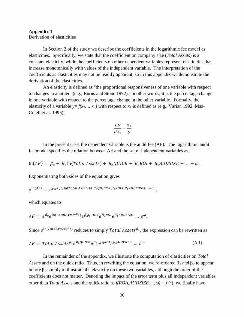
In Section 2 of the study we describe the coefficients in the logarithmic fee model as

elasticities. Specifically, we state that the coefficient on company size (Total Assets) is a

constant elasticity, while the coefficients on other dependent variables represent elasticities that

increase monotonically with values of the independent variable. The interpretation of the

coefficients as elasticities may not be readily apparent, so in this appendix we demonstrate the

derivation of the elasticities.

An elasticity is defined as "the proportional responsiveness of one variable with respect

to changes in another" (e.g., Burns and Stone 1992). In other words, it is the percentage change

in one variable with respect to the percentage change in the other variable. Formally, the

elasticity of a variable y= f(x1,…,xn) with respect to x1 is defined as (e.g., Varian 1992, Mas-

Colell et al. 1995):

In the present case, the dependent variable is the audit fee (AF). The logarithmic audit

fee model specifies the relation between AF and the set of independent variables as

( ) ( ) .

Exponentiating both sides of the equation gives

( ) ( ) ,

which equates to

( ) .

Since ( ) reduces to simply , the expression can be rewritten as

In the remainder of the appendix, we illustrate the computation of elasticities on Total

Assets and on the quick ratio. Thus, in rewriting the equation, we re-ordered 1 and 2 to appear

before 0 simply to illustrate the elasticity on these two variables, although the order of the

coefficients does not matter. Denoting the impact of the error term plus all independent variables

other than Total Assets and the quick ratio as f(ROA,AUDSIZE,…,) = ( ), we finally have

(A.1)

37

( )

The elasticity of audit fees with respect to Total Assets is computed as

The partial derivative of the audit fee equation with respect to Total Assets is given by

( )

so the elasticity becomes

( )

( )

rewritten as

( )

( )

( )

( )

which simplifies to just the constant 1.

The elasticity of audit fees with respect to the quick ratio and all other independent

variables in the model is a bit different from the elasticity of fees with respect to Total Assets,

because Total Assets enters the equation in natural log form. The quick ratio's elasticity is

computed as

The partial derivative of the audit fee equation with respect to the quick ratio is given by

( )

so the elasticity becomes

38

( )

( )

rewritten as

( )

( )

( )

( )

which simplifies to the monotonically increasing function, .

Referring back to the audit fee equation A.1, it becomes apparent that the elasticities

between both Total Assets and audit fees, and the quick ratio and audit fees, describe the

association between audit fees and each of the independent variables. In the case of Total Assets

that elasticity is constant. In the case of the quick ratio and all other independent variables, that

elasticity is monotonically increasing.

39

Appendix 2

Variable definitions

Variable Name Definition

ACQ Indicator variable defined as 1 if the company engaged in any acquisition activities

during the year, and 0 otherwise (Compustat AQP > 0)

AGE Company age. Defined as the number of active years in the Compustat database

AUDCHG Indicator variable defined as 1 if the company changed auditors during the year, and 0

otherwise (from Audit Analytics)

AUDIT FEES Audit fees for the fiscal year (from Audit Analytics)

AUDSIZE Indicator variable defined as 1 if the auditor is a Big-5 firm, 0 otherwise (from Audit

Analytics)

DEBTA Ratio of debt to total assets (Compustat DLTT/AT)

DEBTFIN Indicator variable defined as 1 if the company engaged in any debt financing during the

year, and 0 otherwise (based on Compustat DLTIS > 0)

EX_DISC Indicator variable defined as 1 if the company reported any extraordinary or

discontinued items for the year, and 0 otherwise (based on Compustat XI > 0)

FOR_PCT Percentage of sales from foreign operations (from Compustat segment data)

GC_OPIN Indicator variable defined as 1 if the company received a modification to its audit

opinion, and 0 otherwise (from Audit Analytics)

IC_OPIN

Indicator variable defined as 1 if the company received an adverse opinion due to

material weaknesses in internal controls during the year, and 0 otherwise (from Audit

Analytics)

INVARECA Ratio of inventory plus receivables to total assets (Compustat (RECT + INVT)/AT)

LOSS Indicator variable defined as 1 if the company reported a net loss during the year, and 0

otherwise (based on Compustat NI)

M/B The company's market to book ratio at the beginning of the fiscal year (Compustat

PRCC_F / (CEQ/CSHO))

NONDECYR Indicator variable defined as 1 if the company has a non-December fiscal year end, and

0 otherwise (base on Compustat FYR)

NUMSEGS The square root of the number of operating segments reported (from Compustat

segment data)

OPINLAG Number of days between the end of the company's fiscal year and the date on which the

audit report is issued (from Audit Analytics)

QUICK Quick ratio (Compustat (ACT - INVT) / LCT)

RESTATE Indicator variable defined as 1 if the company was engaged in restatement activities

during the year, 0 otherwise (from Audit Analytics)

RESTR Indicator variable defined as 1 if the company engaged in any restructuring activities

during the year, and 0 otherwise (based on Compustat RCP > 0)

ROA Return on assets (Compustat EBIT/AT)

SOX Indicator variable defined as 1 if the company's controls were audited pursuant to SOX

section 404, and 0 otherwise (from Audit Analytics)

STOCKFIN Indicator variable defined as 1 if the company engaged in any stock financing during

the year, and 0 otherwise (based on Compustat SSTK > 0)

TOTAL ASSETS Total assets (AT)

ZSCORE

Bankruptcy score from Zmijewski (1984), computed as:-4.336 -4.513*ROA

+5.679*Leverage +0.004*Current Ratio. Note that a higher score indicates greater

financial distress. ROA = (NI+TIE)/AT. Leverage = LT/AT. Current Ratio = ACT/LCT

40

TABLE 1

Descriptive statistics

Variable Name Mean Median Minimum Maximum

Standard

Deviation

25th

Percentile

75th

Percentile

AUDIT FEES (in $) 936,013 272,563 2,000 42,200,000 2,186,986 111,000 820,000

TOTAL ASSETS (in $ millions) 1,904.82 147.62 0.00 270,634 8,212 27.24 758.85

Sales (in $ millions) 1,630.19 126.27 0.00 335,086 7,983 19.05 707.41

Market Value (in $ millions) 2,273.03 162.09 0.00 439,013 12,255 26.79 835.39

LN(AUDIT FEES) 12.647 12.516 7.601 17.558 1.433 11.617 13.617

LN(TOTAL ASSETS) 18.725 18.810 6.908 26.324 2.576 17.120 20.447

ACQ 0.036 0 0 1 0.187 0 0

AGE 17.106 12 1 57 13.927 7 22

AUDCHG 0.007 0 0 1 0.084 0 0

AUDSIZE 0.725 1 0 1 0.447 0 1

DEBTTA 0.211 0.086 0.000 91.000 0.994 0.000 0.278

DEBTFIN 0.469 0 0 1 0.499 0 1

EX_DISC 0.222 0 0 1 0.416 0 0

FOR_PCT 0.136 0 0 1 0.234 0 0

GC_OPIN 0.117 0 0 1 0.322 0 0

IC_OPIN 0.027 0 0 1 0.163 0 0

INVARECA 0.256 0.217 0.000 1.000 0.204 0.086 0.378

LOSS 0.458 0 0 1 0.498 0 1

M/B 3.762 1.914 -4,881 8,061 109.411 0.959 3.559

NONDECYR 0.308 0 0 1 0.462 0 1

NUMSEGS 1.213 1.000 0.000 3.464 0.618 1.000 1.732

OPINLAG 66.595 62 0 1,171 48.450 44 77

QUICK 3.070 1.392 0.000 1,907 20.879 0.820 2.674

RESTATE 0.003 0 0 1 0.059 0 0

RESTR 0.220 0 0 1 0.415 0 0

ROA -0.635 0.040 -695 5.175 10.090 -0.132 0.100

SOX 0.232 0 0 1 0.422 0 0

STOCKFIN 0.814 1 0 1 0.389 1 1

ZSCORE 11.228 -1.315 -8,208 37,033 340.389 -2.556 0.139

Notes:

Table 1 shows the basic descriptive statistics on variables used in the paper. Variable descriptions are

provided in Appendix 2. The statistics are restricted to observations with non-missing data on all

variables from 2000 through 2006, comprising 28,326 observations in total. The numbers of

observations per year are shown in Table 2.

41

TABLE 2

Regression of log of fees on log of assets, by year

Model: ln(Audit Feesi) = ln( + ln(Total Assetsi) + ln(i

Year

Number

of Obs

Intercept:

ln(*

Parameter

Estimate: 1*

Model R-

square White Chi-Square

2000 2,715 4.04 0.431 66.5% 19.46 (p<0.0001)

2001 4,220 4.27 0.423 69.9% 49.23 (p<0.0001)

2002 4,414 4.36 0.428 72.0% 47.22 (p<0.0001)

2003 4,439 4.29 0.441 75.6% 58.39 (p<0.0001)

2004 4,420 3.57 0.498 76.4% 22.87 (p<0.0001)

2005 4,362 3.46 0.514 78.2% 35.27 (p<0.0001)

2006 3,756 3.64 0.507 79.2% 32.82 (p<0.0001)

Notes:

* Intercept and parameter estimate are significant at p < 0.0001 each year.

Table 2 shows the size elasticity of audit fees by year (1), along with the explanatory power and

heteroskedasticity statistic from the regression. Note that intercepts in logarithmic fee

regressions in some studies range between 9 and 11. Ours range between 3 and 5. The apparent

difference is due to scaling assets as reported by Compustat prior to computing the natural log.

Compustat reports assets in millions. Audit Analytics reports fees in dollars, so we scale assets

to dollars as well. Since assets are only being adjusted by a fixed multiplier in either case, the

unit of measure has no effect on the parameter estimates in the log form regression or on the

statistical significance of the intercept, but rather only on the scale of the intercept. In other

words, if we leave assets in millions as reported by Compustat, the intercept term in our

regressions ranges from 9 to 11.

42

TABLE 3

Elasticity of fees by year and size group

Model: ln(Audit Feesi) = ln( + ln(Total Assetsi) + ln(i

Panel A: Size elasticity of fees, by year and asset quintile

Quintile 2000 2001 2002 2003 2004 2005 2006

Average

Elasticity

1 0.31 0.29 0.24 0.28 0.25 0.28 0.30 0.28

2 0.34 0.34 0.38 0.45 0.62 0.71 0.62 0.49

3 0.52 0.20 0.28 0.34 0.46 0.57 0.48 0.41

4 0.51 0.53 0.56 0.49 0.41 0.42 0.45 0.48

5 0.57 0.60 0.67 0.64 0.62 0.55 0.53 0.60

Panel B: Size elasticity of fees, by year and asset decile

Decile 2000 2001 2002 2003 2004 2005 2006

Average

Elasticity

Average

Elasticity, with

all control

variables

1 0.31 0.28 0.20 0.18 0.22 0.19 0.23 0.23 0.25

2 0.49 0.28 0.46 0.48 0.31 0.58 0.49 0.44 0.46

3 0.29 0.44 0.27 0.38 0.63 0.80 0.64 0.49 0.40

4 0.25 0.36 0.23 0.47 0.70 0.58 0.41 0.43 0.39

5 0.42 0.10 0.47 0.52 0.55 0.65 0.14 0.41 0.37

6 0.45 0.24 0.33 0.08 0.51 0.65 0.46 0.39 0.36

7 0.95 0.59 0.55 0.54 0.47 0.41 0.49 0.57 0.52

8 0.39 0.55 0.50 0.39 0.33 0.30 0.44 0.41 0.43

9 0.50 0.62 0.67 0.72 0.60 0.47 0.49 0.58 0.54

10 0.64 0.63 0.71 0.69 0.64 0.55 0.54 0.63 0.61

43

TABLE 3 (Continued)

Notes:

Table 3, panels A and B report the coefficients on from the regression model in Equation 2, by year and size group (defined by total

assets). For consistency in the paper, we generally define size groups at the asset quintile level, although panel B above also reports

the more finely detailed partition at the decile level. Both tables show that audit fees do not exhibit constant elasticity with regard to

size, but rather exhibit lower elasticity among small clients, and higher elasticity among large clients. In addition, the final column of

panel B reports the coefficient on size from the regression with a full set of control variables (Equation 5), illustrating that the trend in

size elasticity of fees is the same with or without control variables.

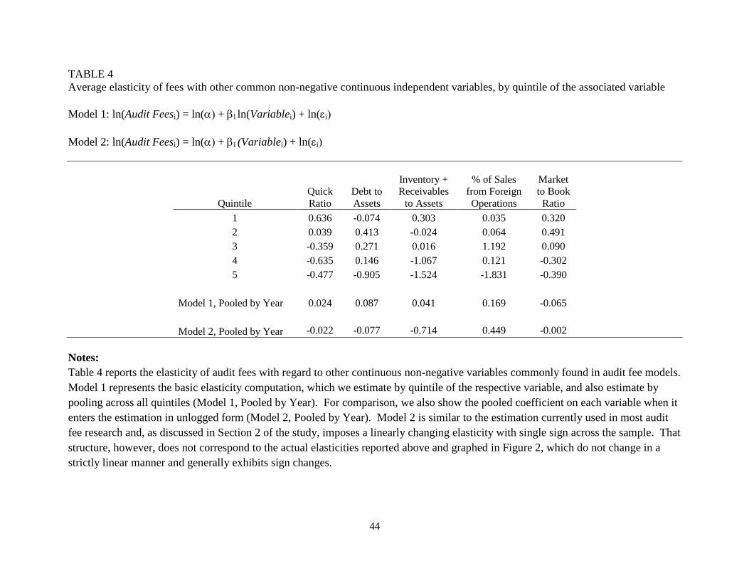
44

TABLE 4

Average elasticity of fees with other common non-negative continuous independent variables, by quintile of the associated variable

Model 1: ln(Audit Feesi) = ln( + ln(Variablei) + ln(i

Model 2: ln(Audit Feesi) = ln( + (Variablei) + ln(i

Quintile

Quick

Ratio

Debt to

Assets

Inventory +

Receivables

to Assets

% of Sales

from Foreign

Operations

Market

to Book

Ratio

1 0.636 -0.074 0.303 0.035 0.320

2 0.039 0.413 -0.024 0.064 0.491

3 -0.359 0.271 0.016 1.192 0.090

4 -0.635 0.146 -1.067 0.121 -0.302

5 -0.477 -0.905 -1.524 -1.831 -0.390

Model 1, Pooled by Year 0.024 0.087 0.041 0.169 -0.065

Model 2, Pooled by Year -0.022 -0.077 -0.714 0.449 -0.002

Notes:

Table 4 reports the elasticity of audit fees with regard to other continuous non-negative variables commonly found in audit fee models.

Model 1 represents the basic elasticity computation, which we estimate by quintile of the respective variable, and also estimate by

pooling across all quintiles (Model 1, Pooled by Year). For comparison, we also show the pooled coefficient on each variable when it

enters the estimation in unlogged form (Model 2, Pooled by Year). Model 2 is similar to the estimation currently used in most audit

fee research and, as discussed in Section 2 of the study, imposes a linearly changing elasticity with single sign across the sample. That

structure, however, does not correspond to the actual elasticities reported above and graphed in Figure 2, which do not change in a

strictly linear manner and generally exhibits sign changes.

45

TABLE 5

Comparison of explained variance from the fee regression model

Model (Equation 5):

LN(Audit Fees)i,t = a + β1LN(TotalAssets)i,t + β2AUDSIZEi,t + β3AUDCHGi,t + β4NONDECYRi,t + β5OPINLAGi,t +

β6GC_OPINi,t + β7B/Mi,t + β8SOXi,t + β9IC_OPINi,t + β10QUICKi,t + β11STOCKFINi,t + β12DEBTFINi,t + β13INVARECAi,t +

β14EX_DISCi,t + β15DEBTAi,t + β16ROAi,t + β17LOSSi,t + β18NUMSEGSi,t + β19FOR_PCTi,t + β20ACQi,t +β21RESTRi,t +

β22RESTATEi,t + β23ZSCOREi,t + β24AGEi,t + Industry Dummies + εi,t

Pooled Sample with

Year Dummies By Year

By Year and Asset

Quintile

By Year and Asset

Decile

ln(Fees) Fees ln(Fees) Fees ln(Fees) Fees ln(Fees) Fees

Year

82.3% 50.8%

2000

75.7% 34.3% 79.7% 44.5% 81.2% 45.8%

2001

78.2% 46.6% 82.1% 64.9% 82.9% 70.9%

2002

79.8% 22.0% 83.3% 46.1% 84.4% 73.4%

2003

81.9% 49.4% 85.2% 69.9% 86.0% 68.8%

2004

86.1% 53.3% 88.1% 65.7% 88.7% 66.8%

2005

85.9% 67.6% 87.7% 67.9% 88.4% 68.3%

2006

86.9% 67.1% 88.5% 75.3% 89.2% 76.4%

Notes:

Table 5 reports the explained variance from the full regression model (Equation 5) by year, by year and asset quintile, and by year and

asset decile. The explanatory power for ln(Fees) is the r-square reported from the regression. Note that we are not comparing two

models here, but rather illustrating that the unexplained variance in the log of fees is not synonymous with the unexplained variance in

fees. This difference is due both to the natural compression derived from the log transformation discussed in Section 2 of the study,

and the median shift discussed in Section 3. Since fees do not exhibit constant elasticity with respect to size (defined as total assets),

and since size provides most of the explanatory power of the model, the table also illustrates that the variance in fees captured in the

log-log regression improves as size groups become more homogeneous in the estimation.

46

TABLE 6

Coefficients on audit firm size (AUDSIZE) from the audit fee regression specified in Equation 5,

by year and asset quintile

Model (Equation 5):

LN(Audit Fees)i,t = a + β1LN(TotalAssets)i,t + β2AUDSIZEi,t + β3AUDCHGi,t + β4NONDECYRi,t

+ β5OPINLAGi,t + β6GC_OPINi,t + β7B/Mi,t + β8SOXi,t + β9IC_OPINi,t + β10QUICKi,t +

β11STOCKFINi,t + β12DEBTFINi,t + β13INVARECAi,t + β14EX_DISCi,t + β15DEBTAi,t + β16ROAi,t

+ β17LOSSi,t + β18NUMSEGSi,t + β19FOR_PCTi,t + β20ACQi,t +β21RESTRi,t + β22RESTATEi,t +

β23ZSCOREi,t + β24AGEi,t + Industry Dummies + εi,t

Quintile

Year 1 2 3 4 5

2000 0.117 0.203 0.164 0.132 -0.386

0.0214 0.0005 0.0730 0.3767 0.0965

2001 0.312 0.192 0.062 0.139 -0.204

0.0000 0.0000 0.2503 0.2735 0.1860

2002 0.485 0.333 0.099 0.220 -0.093

0.0000 0.0000 0.0576 0.0784 0.5911

2003 0.488 0.356 0.291 0.121 -0.033

0.0000 0.0000 0.0000 0.2483 0.8417

2004 0.707 0.456 0.396 0.325 -0.062

0.0000 0.0000 0.0000 0.0005 0.6512

2005 0.684 0.429 0.345 0.288 0.087

0.0000 0.0000 0.0000 0.0000 0.5142

2006 0.612 0.430 0.279 0.194 -0.057

0.0000 0.0000 0.0000 0.0041 0.6894

Notes:

Table 6 reports the coefficients on AUDSIZE (2) from the estimation of Equation 5 by year and

asset quintile. For each year and quintile pair, the coefficient is reported on top (in boldface) and

the 2-sided p-value is reported on bottom. In the lowest two asset quintiles, the coefficients on

AUDSIZE show that Big 5 audit firms are significantly associated with higher fees in each year.

In the third quintile, the coefficients on AUDSIZE are positive and significant at conventional

levels in all years except 2001. The association is weaker in the fourth quintile, where the

coefficients are always positive, but significant at conventional levels in only four of the seven

years. In the largest quintile, the association actually flips sign in all years but 2005, and is

statistically significant at conventional levels in 2000 and marginally significant in 2001.

Further, even among the first three quintiles where the association is generally strongly positive,

the magnitude of the association decreases monotonically with each quintile.

47

TABLE 7

Replication of association between auditor change and audit fees, from Ghosh and Lustgarten

2006, Table 4 Panel A

Ghosh & Lustgarten

Table 4 Replication

Ghosh & Lustgarten

By Asset Quintile

Table 4 Replication

Using Our Equation 5

Coefficient p-value

Coefficient p-value

Pooled -0.09 0.0001

-0.06 0.0001

Quintile 1

0.06 0.0188

Quintile 2

-0.12 0.0001

Quintile 3

-0.08 0.0060

Quintile 4

-0.13 0.0001

Quintile 5 -0.05 0.2370

Notes:

Table 7 reports the association between auditor change and audit fees, taken from Table 4 of

Ghosh and Lustgarten (2006), using their data period from 2000 to 2003. The leftmost two

columns report the coefficient on auditor change (AUDCHG) using their model, and pooling the

data across all five quintiles of asset size. The rightmost two columns report the coefficients

using our model from Equation 5, both pooled and run separately by asset quintile. In the

interest of brevity, we have limited the table to report only the primary variable of interest,

auditor change. The replications pooled across asset size using either model provide identical

inferences to those reported by Ghosh and Lustgarten. Examining the association in more finely

partitioned client groups however, shows that the negative association reported in their overall

result, and more widely throughout the body of audit research, varies substantially with client

size. Among the smallest quintile of clients, not only do the clients not experience a fee

reduction, but in fact see a fee increase.

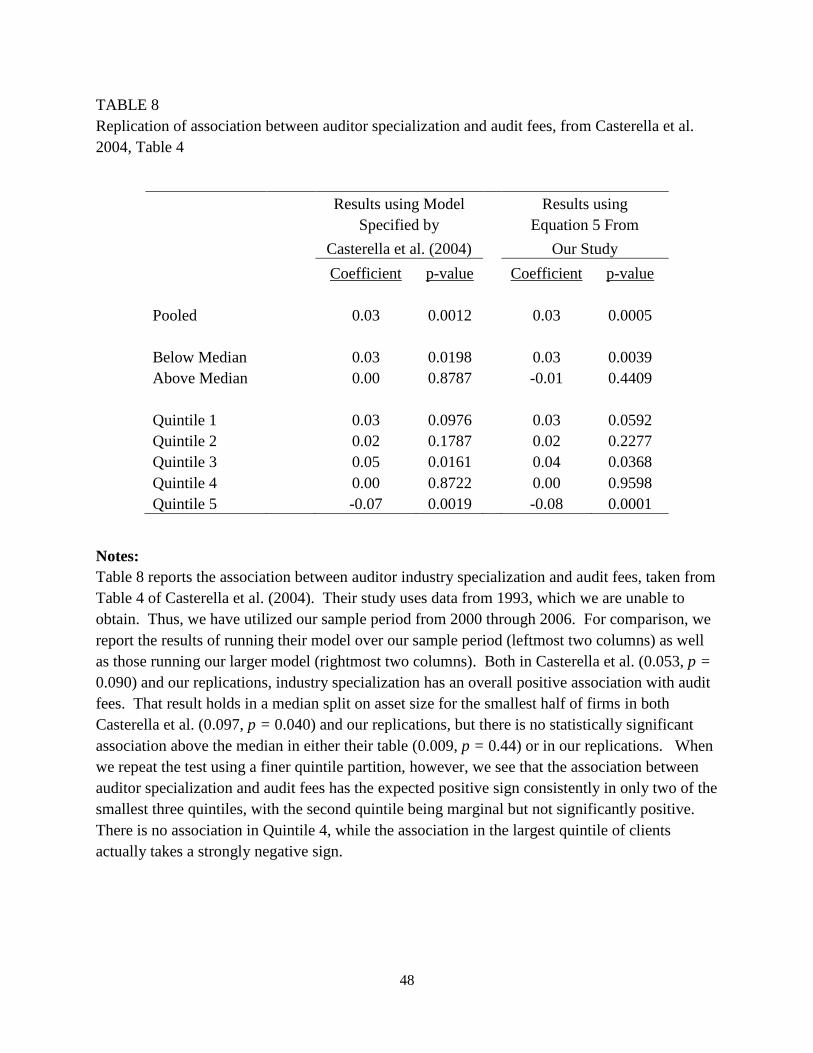
48

TABLE 8

Replication of association between auditor specialization and audit fees, from Casterella et al.

2004, Table 4

Results using Model Results using

Specified by

Equation 5 From

Casterella et al. (2004)

Our Study

Coefficient p-value

Coefficient p-value

Pooled

0.03 0.0012

0.03 0.0005

Below Median

0.03 0.0198

0.03 0.0039

Above Median

0.00 0.8787

-0.01 0.4409

Quintile 1

0.03 0.0976

0.03 0.0592

Quintile 2

0.02 0.1787

0.02 0.2277

Quintile 3

0.05 0.0161

0.04 0.0368

Quintile 4

0.00 0.8722

0.00 0.9598

Quintile 5 -0.07 0.0019 -0.08 0.0001

Notes:

Table 8 reports the association between auditor industry specialization and audit fees, taken from

Table 4 of Casterella et al. (2004). Their study uses data from 1993, which we are unable to

obtain. Thus, we have utilized our sample period from 2000 through 2006. For comparison, we

report the results of running their model over our sample period (leftmost two columns) as well

as those running our larger model (rightmost two columns). Both in Casterella et al. (0.053, p =

0.090) and our replications, industry specialization has an overall positive association with audit

fees. That result holds in a median split on asset size for the smallest half of firms in both

Casterella et al. (0.097, p = 0.040) and our replications, but there is no statistically significant

association above the median in either their table (0.009, p = 0.44) or in our replications. When

we repeat the test using a finer quintile partition, however, we see that the association between

auditor specialization and audit fees has the expected positive sign consistently in only two of the

smallest three quintiles, with the second quintile being marginal but not significantly positive.

There is no association in Quintile 4, while the association in the largest quintile of clients

actually takes a strongly negative sign.

49

Figure 1a Audit fees vs. total assets (fees <= $20 million and assets <= $60 billion)

Figure 1b Log of audit fees vs. log of total assets (fees <= $20 million and assets <= $60 billion)

50

Figure 2 The relationship between fees and other common non-negative continuous independent variables

Figure 2a Elasticity of fees to quick ratio by quick ratio

quintile

Figure 2b Elasticity of fees to debt to assets by debt to assets

quintile

Figure 2c Average log of fees by quick ratio decile Figure 2d Average log of fees by debt to assets decile

-1.000

-0.800

-0.600

-0.400

-0.200

0.000

0.200

0.400

0.600

0.800

0 2 4 6

Elas

tici

ty

Quick Quintile

Quick Elasticities

Model 1 QuintileElasticities

Model 2 PooledPredictions

-1.000

-0.800

-0.600

-0.400

-0.200

0.000

0.200

0.400

0.600

0 2 4 6

Elas

tici

ty

Debt to Assets Quintile

Debt to Assets Elasticities

Model 1 QuintileElasticities

Model 2 PooledPredictions

10.5

11

11.5

12

12.5

13

13.5

1 2 3 4 5 6 7 8 9 10

Logg

ed F

ees

Quick Decile

Logged Fees by Quick Decile

11.5

12

12.5

13

13.5

1 2 3 4 5 6 7 8 9 10

Logg

ed F

ees

Debt to Assets Decile

Logged Fees by Debt to Assets Decile

51

Notes:

Figure 2 shows the relationship between fees and other common continuous, non-negative predictor variables. Figures 2a and 2b

show the average elasticity of fees to quick ratio and debt to assets based on yearly regressions by quintiles of the respective variable,

using the logged variable as the regressor (Model 1 quintile results in Table 4). The figures also show the estimated elasticity for each

quintile based on yearly pooled regressions using the respective unlogged variable as the regressor (using the Model 2 results in Table

4), the common methodology in audit fee estimation. Linear and polynomial estimations are provided for the Model 1 quintile results

and a linear estimation is provided for the Model 2 results. Figures 2c and 2d show average logged audit fees as a function of quick

ratio and debt to asset deciles, respectively. The patterns in the graphs clearly correspond to the Model 1 quintile results in Figures 2a

and 2b.

52

Figure 3 Log of audit fee vs. student residual (simple regression)

53

Figure 4a Mean regression residuals by company size - full sample versus quintile and decile

estimations

Figure 4b Mean regression residual by company size - full sample versus median split

estimations

-0.2000

-0.1000

0.0000

0.1000

0.2000

0.3000

0.4000

1 2 3 4 5 6 7 8 9 10 11 12 13 14 15 16 17 18 19 20

Me

an r

egr

ess

ion

re

sid

ual

Rank of Company Size

Full PooledRegression

Regression byDecile

Regression byQuintile

-0.2000

-0.1000

0.0000

0.1000

0.2000

0.3000

0.4000

1 2 3 4 5 6 7 8 9 10 11 12 13 14 15 16 17 18 19 20Me

an r

egr

ess

ion

re

sid

ual

Rank of Company Size

Full PooledRegression

Regressionby Median