Audiovisual Speech Source Separation: An overview of key ...
19
HAL Id: hal-00990000 https://hal.archives-ouvertes.fr/hal-00990000 Submitted on 13 May 2014 HAL is a multi-disciplinary open access archive for the deposit and dissemination of sci- entific research documents, whether they are pub- lished or not. The documents may come from teaching and research institutions in France or abroad, or from public or private research centers. L’archive ouverte pluridisciplinaire HAL, est destinée au dépôt et à la diffusion de documents scientifiques de niveau recherche, publiés ou non, émanant des établissements d’enseignement et de recherche français ou étrangers, des laboratoires publics ou privés. Audiovisual Speech Source Separation: An overview of key methodologies Bertrand Rivet, Wenwu Wang, Syed Mohsen Naqvi, Jonathon Chambers To cite this version: Bertrand Rivet, Wenwu Wang, Syed Mohsen Naqvi, Jonathon Chambers. Audiovisual Speech Source Separation: An overview of key methodologies. IEEE Signal Processing Magazine, Institute of Electri- cal and Electronics Engineers, 2014, 31 (3), pp.125-134. 10.1109/MSP.2013.2296173. hal-00990000
Transcript of Audiovisual Speech Source Separation: An overview of key ...
HAL Id: hal-00990000https://hal.archives-ouvertes.fr/hal-00990000
Submitted on 13 May 2014
HAL is a multi-disciplinary open accessarchive for the deposit and dissemination of sci-entific research documents, whether they are pub-lished or not. The documents may come fromteaching and research institutions in France orabroad, or from public or private research centers.
L’archive ouverte pluridisciplinaire HAL, estdestinée au dépôt et à la diffusion de documentsscientifiques de niveau recherche, publiés ou non,émanant des établissements d’enseignement et derecherche français ou étrangers, des laboratoirespublics ou privés.
Audiovisual Speech Source Separation: An overview ofkey methodologies
Bertrand Rivet, Wenwu Wang, Syed Mohsen Naqvi, Jonathon Chambers
To cite this version:Bertrand Rivet, Wenwu Wang, Syed Mohsen Naqvi, Jonathon Chambers. Audiovisual Speech SourceSeparation: An overview of key methodologies. IEEE Signal Processing Magazine, Institute of Electri-cal and Electronics Engineers, 2014, 31 (3), pp.125-134. �10.1109/MSP.2013.2296173�. �hal-00990000�
1
Audio-Visual Speech Source Separation
Bertrand Rivet, Wenwu Wang, Syed Mohsen Naqvi and Jonathon A. Chambers
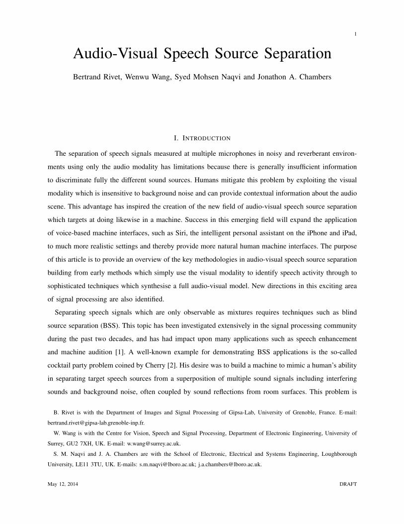
I. INTRODUCTION
The separation of speech signals measured at multiple microphones in noisy and reverberant environ-
ments using only the audio modality has limitations because there is generally insufficient information
to discriminate fully the different sound sources. Humans mitigate this problem by exploiting the visual
modality which is insensitive to background noise and can provide contextual information about the audio
scene. This advantage has inspired the creation of the new field of audio-visual speech source separation
which targets at doing likewise in a machine. Success in this emerging field will expand the application
of voice-based machine interfaces, such as Siri, the intelligent personal assistant on the iPhone and iPad,
to much more realistic settings and thereby provide more natural human machine interfaces. The purpose
of this article is to provide an overview of the key methodologies in audio-visual speech source separation
building from early methods which simply use the visual modality to identify speech activity through to
sophisticated techniques which synthesise a full audio-visual model. New directions in this exciting area
of signal processing are also identified.
Separating speech signals which are only observable as mixtures requires techniques such as blind
source separation (BSS). This topic has been investigated extensively in the signal processing community
during the past two decades, and has had impact upon many applications such as speech enhancement
and machine audition [1]. A well-known example for demonstrating BSS applications is the so-called
cocktail party problem coined by Cherry [2]. His desire was to build a machine to mimic a human’s ability
in separating target speech sources from a superposition of multiple sound signals including interfering
sounds and background noise, often coupled by sound reflections from room surfaces. This problem is
B. Rivet is with the Department of Images and Signal Processing of Gipsa-Lab, University of Grenoble, France. E-mail:
W. Wang is with the Centre for Vision, Speech and Signal Processing, Department of Electronic Engineering, University of
Surrey, GU2 7XH, UK. E-mail: [email protected].
S. M. Naqvi and J. A. Chambers are with the School of Electronic, Electrical and Systems Engineering, Loughborough
University, LE11 3TU, UK. E-mails: [email protected]; [email protected].
May 12, 2014 DRAFT
2
usually addressed within the framework of convolutive BSS taking into account room reverberations in
the separation model. In this framework, the vector observations x(t) are modeled as a linear convolutive
mixture of the vector sources s(t): x(t) = H(t) ∗ s(t), where H(t) is the matrix of impulse responses
between each source and each mixture, and t is the discrete time index. For simplicity, H(t) is assumed
to be square so that the number of microphones and sources is equal, but this is not necessary to achieve
separation. The aim is thus to estimate the demixing matrix W (t) so that s(t) = W (t) ∗x(t) contains an
estimate of each source si(t), where subscript i is the index of the source. Alternatively, it is solved in a
transform domain by converting the full-band speech mixtures into sub-band components which are then
separated either individually or jointly, leading to a computationally more efficient method, e.g. frequency
domain BSS. In this latter case, assuming static sources, the frequency domain counterparts of mixing
and demixing equations are x(m, f) = H(f)s(m, f) and s(m, f) = W (f)x(m, f), respectively, where
·(m, f) is the short-term discrete-time Fourier transform (STFT) of ·(t), ·(f) is the Fourier transform of
·(t), and m and f are the time frame and frequency bin indices respectively. This however introduces
the permutation and scaling ambiguity problems, due to the potentially inconsistent orders and scales of
the separated source components at the individual frequency bands that are inherent to the instantaneous
BSS models: in other words, W (f) = Λ(f)P (f)H(f)−1, where Λ(f) is a diagonal matrix (i.e. modeling
the scaling indeterminacy) and P (f) is a permutation matrix (i.e. modeling the permutation ambiguity).
Many methods have, therefore, been developed to mitigate these ambiguities before reconstructing the
full-band source signals (more details can be found in [1]). A more recent approach is independent vector
analysis (IVA) whereby the permutation problem is mitigated via a coupling of the adaptation across all
the frequency bands [29].
These convolutive BSS techniques can be broadly attributed to a category of linear filtering based
methods. Another powerful method for separating convolutive mixtures is based on a form of time-
varying filtering using time-frequency (T-F) masking where the aim is to form a probabilistic (soft) or
binary (hard) mask M(m, f) for each source, and then applying the mask to the T-F representation of
the mixtures for the extraction of that source: s(m, f) = M(m, f)x(m, f). The mask can be estimated
by the evaluation of various cues from the mixtures, such as statistical, spatial, temporal and/or spectral
cues, using an expectation maximization (EM) algorithm [3] under a maximum likelihood or a Bayesian
framework. The T-F masking techniques can often be applied directly on underdetemined mixtures for the
extraction of a larger number of sources than the observed signals. Despite these efforts and the promising
progress made in this area, the state-of-the-art algorithms commonly suffer in the following two practical
situations: namely, highly reverberant and noisy environments, and when multiple moving sources are
May 12, 2014 DRAFT

3
present. For example, most existing methods of frequency domain BSS are practically constrained by
the data length limitation, i.e. the number of samples available at each frequency bin is not sufficient for
learning algorithms to converge [4], while the various cues, such as the spatial cues which are used to
calculate the likelihood of the source being present for the T-F mask estimation, become more ambiguous
with the increasing reverberation and background noise. The performance of most existing algorithms
degrades substantially in these adverse acoustic environments.
The methods mentioned above exploit only single modality signals in the audio domain. However, it is
now widely accepted that human speech is inherently at least bimodal involving interactions between audio
and visual modalities [5]. For example, the uttering activities are often coupled with the visual movements
of vocal organs, while reading lip movement can help a human to infer the meaning of a spoken
sentence in a noisy environment [6]. The well-known McGurk effect also confirms that visual articulatory
information is integrated into the human speech perception process automatically and unconsciously [7].
For example, under certain conditions, a visual /ga/ combined with an auditory /ba/ is often heard as
/da/. As also suggested by Cherry [2], fusing the audio-visual (AV) information from different sensory
measurements would be the best way to address the machine cocktail party problem. The intrinsic AV
coherence1 has been exploited previously to improve the performance of automatic speech recognition [8]
and identification [9].
In the study in [10], a speech signal corrupted by white noise is enhanced with filters estimated from
the video input. The aim is to estimate a time-varying Wiener filter based on a linear regression (linear
predictive coding, LPC) between the audio and visual signals from a regressor trained with a clean
database (Figure 1) and therefore is termed an AV-Wiener filter. This preliminary study has been shown
to be efficient on very simple data (succession of vowels and consonants). For instance, with an input
signal-to-noise ratio (SNR) of -18dB, a simple linear discriminant analysis of the filtered signals leads
to a word classification accuracy (CA) of 40% after the AV enhancement compared to the CA of 10%
with the classical audio enhancement while the unfiltered data leads to a CA of 5%. However, due to the
complex relationship between audio and video signals, this simple approach is found to have limitations
when applied on more complex signals such as natural speech and other noise sources. Nevertheless,
this pioneering approach has shown that it can be extremely beneficial to combine video information
1Here we use the term coherence to describe the dependency between the audio and visual modalities, to be consistent with
the conventional use of the term in previous works in the literature, such as [10]–[12], [27]. As discussed in subsequent sections,
the dependency can be modelled as either joint distribution of the AV features or joint AV atoms (i.e. signal components).
May 12, 2014 DRAFT

4
LPC enhanced filter
Enhanced audio
LPC Inverse filter
Noisy audio
Residual signal
LW
LH
A
AV
V
Estimation
Fig. 1. Audio visual estimation of Wiener filter from [10]. The linear predictive coding (LPC) method is used to model the
noisy speech. The audio feature based on LPC inverse filtered spectrum is fused with the visual features such as the lip width
(LW) and height (LH) for enhancing the LPC spectrum of the noisy speech. The enhanced speech signal can therefore be
obtained based on this LPC enhanced filter and the residual signal obtained from the inverse filtering of the noisy speech.
when dealing with speech enhancement mirroring the advantage gained in automatic speech recognition
systems [8].
During the last decade, integrating visual information into an audio-only speech source separation
system has been emerging as an exciting new area in signal processing: audio-visual (i.e. multimodal)
speech source separation [11]. The activities in this area include robust modelling of AV coherence [12],
[13]; fusing of AV coherence with independent component analysis (ICA) or T-F masking [14]; using
AV coherence to resolve ambiguities in BSS [13], [15]; employing visual information for the detection of
voice activities [16], [17]; exploiting redundancy within the AV data to design efficient speech separation
algorithms based on sparse representations [14], [18]; and more recently, audio-visual scene analysis for
addressing the challenging problem of speech separation from moving sources [4], [19] or in environments
with long reverberation time [20].
A large diversity of approaches to tackle the speech source separation problem using both audio
and visual modalities has therefore clearly been developed. To present these in a coherent manner the
remainder of this tutorial is organized according to the increasing sophistication in the way in which video
is used to help speech source enhancement as summarized in Table I. The advantages and disadvantages
of the methods are also highlighted in the table, and references are added to papers where the full details
can be found of experimental studies which present the performance gains achievable by adding video
in the processing.
May 12, 2014 DRAFT
5
Methods Main advantages Main disadvantages
Det
ail
of
AV
rep
rese
nta
tio
n
Bin
ary
Sec
.II
Spectral subtraction [21],
[22]
Effective in noise reduction; Easy to
implement
Introduces processing artefacts; Diffi-
cult to estimate the noise power for
nonstationary signals
AV post-processing of au-
dio ICA [15]
Low computational cost; Strength of
ICA framework; Correct (almost) all
permutations
Increases delay (i.e. latency); Potential
processing artefacts
Extraction based on tempo-
ral voice activity [16]
Low computational cost; Simple as-
sumptions
Limited to low reverberation
Vis
ual
Sce
ne
An
aly
sis
Sec
.II
I AV beamform-
ing/ICA/IVA [4], [19],
[23]–[25]
Potential for separating moving
sources; Correct the permutations;
Improve convergence of ICA/IVA
algorithms
Degrades with high reverberations
AV T-F masking [20] Exploits time-varying property
of sources; Not affected by the
permutation problem
High computational complexity; Chal-
lenging in resolving spectral overlaps
Fu
lljo
int
AV
mo
del
Sec
.I AV-Wiener filter [10] Low computational cost Limited to simple signals; Difficulty in
learning accurate AV model
Sec
.IV
-A
Maximization of AV likeli-
hood [11], [26]
Can extract speech sources from under-
determined mixtures
Limited to instantaneous mixtures; Dif-
ficulty in learning accurate AV model;
AV Regularization of
ICA [27]
Exploiting the strength of the ICA
framework
Limited improvement compared to au-
dio only ICA in particular for convolu-
tive mixtures
AV post-processing of au-
dio ICA [12]
Moderate computational cost Difficulty of learning accurate AV
model; Increases delay (i.e. latency)
Sec
.IV
-B AVDL + T-F masking [14] Can capture the local information
within the signals; Not affected by the
permutation problem
High computational complexity; Only
bimodality informative parts of the sig-
nals are learned
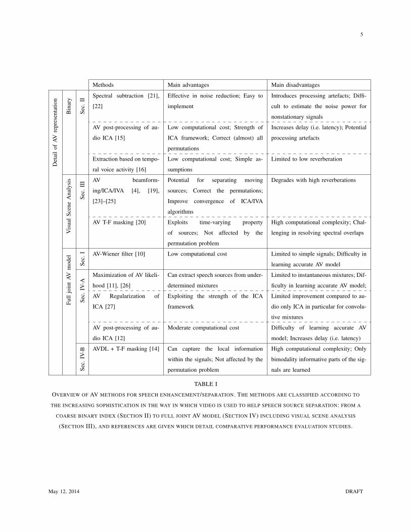
TABLE I
OVERVIEW OF AV METHODS FOR SPEECH ENHANCEMENT/SEPARATION. THE METHODS ARE CLASSIFIED ACCORDING TO
THE INCREASING SOPHISTICATION IN THE WAY IN WHICH VIDEO IS USED TO HELP SPEECH SOURCE SEPARATION: FROM A
COARSE BINARY INDEX (SECTION II) TO FULL JOINT AV MODEL (SECTION IV) INCLUDING VISUAL SCENE ANALYSIS
(SECTION III), AND REFERENCES ARE GIVEN WHICH DETAIL COMPARATIVE PERFORMANCE EVALUATION STUDIES.
May 12, 2014 DRAFT

6
II. METHODS BASED ON VISUAL VOICE ACTIVITY
A very simple approach to model the link between audio and video signals is to utilise the voice
activity of the time domain speech signal. Indeed, there exist pauses during natural speech: for instance,
during breathing or before a plosive (such as /p/). Such silences can importantly be partially predicted by
the movements of the lips [17]. Based on this idea, several purely video based voice activity detectors (V-
VADs) have been developed [28]: they are generally based on the velocity of face features, usually motions
of the lips. The main advantage of such V-VADs compared to an audio VAD is that they are not corrupted
by concurrent audio sources such as environmental noise, or other speakers. It is worth noting that such
models do not aim at linking audio and video features but they try to infer very coarse information on
silence (i.e. the probability that speech is present P (si(t) 6= 0|ζvi (t))) or not (i.e. P (si(t) = 0|ζvi (m)))
in the audio modality from the video one, where ζvi (t) is the visual signal associated with the ith source
si(t). Examples of speech enhancement methods which exploit a V-VAD are discussed next.
A. Spectral subtraction
A simple method is to extend classical spectral subtraction by embedding visual features [21], [22]: the
spectrum of the enhanced signal is expressed as |s(m, f)|2 = |x(m, f)|2−α|d(m, f)|2, where x(m, f) is
the STFT of a measured microphone signal x(t), d(m, f) is the estimated interference noise spectrum and
α is a parameter to adjust the subtraction level. The spectrum of the interference noise d(m, f) is estimated
from the windows related to the silence of the target source (i.e., the set Ti = {t |P (si(t) = 0|ζvi (t))}).
These windows are efficiently detected by a V-VAD which is thus not corrupted by the interfering audio
noise.
B. AV post-processing of audio ICA
Another use of such high level information (speech/non speech frames) is to embed it into the efficient
ICA framework. In this method, the visual information is used as post-processing after applying an audio
ICA algorithm. Frequency domain source separation generally suffers from the permutation indeterminacy
at each frequency bin: the ICA framework allows the recovery of the sources up to a global permutation
(i.e. the order of the estimated sources is arbitrary). As a consequence, to recover the sources, this
issue must be solved (i.e., permutation matrices P (f) must be the same for all f ). A very intuitive and
efficient method is thus to estimate the permutations in relation to the output power of the sources [15].
Indeed, the V-VAD provides a binary indicator which shows when a specific speaker is silent. Using
this information, one can then solve the permutation indeterminacy by simply minimizing the power
May 12, 2014 DRAFT

7
of the target source during these frames. This method thus exploits the AV dependence, i.e. the joint
distribution of AV features, in a very minimal way but it has been shown to cancel almost all the
permutation ambiguities. Compared to purely audio methods, this requires relatively low computational
cost to mitigate the permutation ambiguities and allows the extraction of only a specific speech source
instead of trying to recover all the sources.
C. AV extraction based on temporal speech activity
A more effective use of such high level information (speech/non speech frames) is to directly incorpo-
rate it into a separation criterion [16] to extract particular speakers in order to provide even less compu-
tational cost than ICA methods. Indeed, considering a set of time samples T so that the sources can be
split into silent ones (∀i ∈ Ssilent, ∀t ∈ T , si(t) = 0) and active ones (∀i ∈ Sactive, ∀t ∈ T , si(t) 6= 0),
purely audio algebraic methods based on generalized eigen decomposition of two covariance matrices
can identify (i) the number of silent speakers (i.e. the cardinality of Ssilent), (ii) the associated support
subspace (i.e. the subspace spanned by {si}i∈Ssilent). In other words, considering any time samples
including some not in T (i.e. the sources in Ssilent can become active), the projection of the audio
recordings x(t) onto the latter identified subspace cancels all sources in Sactive while sources in Ssilent
remain unchanged. However, this method can not identify which source is silent and thus cannot be used
to extract a specific speaker. To overcome this, a weighted kernel principal component analysis can be
used to improve this approach where the weights are a mixture between the audio probability of silence
(given by the eigen values) and the video probability of silence provided by the V-VAD for a particular
speaker [16]. This simple property provides a very efficient and elegant AV method to extract speech
sources.
III. VISUAL SCENE ANALYSIS BASED METHODS
In the previous section, AV extraction methods use the visual modality in a very coarse way: simple
binary information defining silence or not of specific speakers. In this section, this extra modality is used
in a deeper way by visually analyzing the scene for speech enhancement [23], [24]. Such visual scene
analysis thereby informs the source separation algorithms of the locations of the speakers, especially
when dealing with moving sources, which is a more challenging issue since the mixing filters are now
time-varying. Thus, the classical ICA framework may be ineffective due to the large number of time
samples required to accurately estimate the statistics of the mixtures. These methods are implemented in
two stages: mainly video scene analysis (VSA) based on multiple human tracking (MHT) to estimate the
May 12, 2014 DRAFT

8
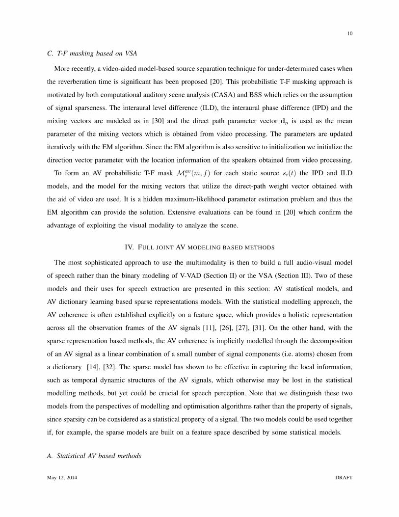
Fig. 2. Block diagram of visual scene analysis based method for speech enhancement. Video localization is based on face and
head detection. A video tracker is implemented for tracking of multiple humans and based on the MCMC-PF. The output of the
video processing is position, direction of arrival, and/or velocity information. On the basis of the visual scene the pre-processed
audio mixtures are separated either by a data independent beamformer or intelligently initialized video-aided source separation
method. Finally, post-processing is applied to enhance the separated audio sources.
position, direction of arrival and velocity information of the people in a room or enclosed environment;
and audio source separation depending on the scene as illustrated in the schematic diagram in Figure 2.
A. Video processing for multiple human tracking
Video based face and head detection is applied for multi-person observations from a single image
as initialization. Then a Markov chain Monte Carlo based particle filter (MCMC-PF) is used for MHT
in the video. More details of the three important parts of the probabilistic MHT: the state model, the
measurement model and the sampling mechanism are provided in [4]. Contrary to the V-VAD described
in Section II, it is highlighted that the full-frontal close-up views of the faces of the speakers, which
are generally not available in a room or an enclosed environment, are not required for these trackers.
The above mentioned MHT methods provide a very good framework for AV scene modeling for source
separation: the output of the video based tracker is 3-D position of each speaker p, the elevation (θp)
and azimuth (βp) angles of arrival to the center of the microphone array. The direct-path weight vector
dp(f, θp, βp) can then be computed for frequency bin f and for source of interest (SOI) p = 1, · · · , P
and the velocity information which can then be used in the AV source separation scheme.
May 12, 2014 DRAFT

9
B. AV source separation of moving sources
Speech source separation is a challenging issue when dealing with moving sources [24]. The proposed
extraction of a particular speaker in an AV context depends on the velocity of this speaker.
1) Physically moving sources: After video scene analysis, if the people are moving then the challenge
of separating respective audio sources is that the mixing filters are time varying; as such the unmixing
filters should also be time varying but these are difficult to determine from only audio measurements.
In [19], a multi-stage method has been developed for speech separation of moving sources based on
VSA. This method consists of several stages including the DOA tracking of speech sources based on
video processing, separation of sources based on beamforming with the beampatterns generated by the
DOAs, and time frequency masking as post-processing. From the video signal, the direct path parameter
vector dp can be obtained, as discussed above, which is then used for the design of a robust least squares
frequency invariant data independent (RLSFIDI) beamformer in order to separate the audio sources. The
T-F masking is used as post-processing to further improve the separation quality of the beamformer by
reducing the interferences to a much lower level. However, such time-varying filtering techniques may
introduce musical noise due to the inaccurate estimate of the mask at some T-F points. To overcome this
problem, smoothing techniques such as cepstral smoothing may be used as in [19].
2) Physically stationary sources: After video processing if the speakers are judged to be physically sta-
tionary for at least two seconds then the direct path parameter vector dp with the whitening matrix obtained
from the audio mixtures is used to intelligently initialize the learning algorithms, such as FastICA/IVA
(many learning algorithms are sensitive to initializations) [4], [29], which solves the inherent permutation
problem in ICA or block permutation in IVA algorithms and yields improved convergence [25].
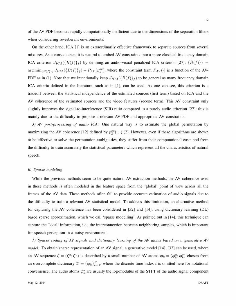
Fig. 3. Speech recording is obtained from two microphones. The direct path parameter vector is calculated with the help of
video cameras. The ILD, the IPD and the mixing vectors which utilize the direct path parameter vector are used to estimate the
model parameters with the EM algorithm. The final probabilistic mask formed from the resulting probabilistic model is used
for source separation.
May 12, 2014 DRAFT
10
C. T-F masking based on VSA
More recently, a video-aided model-based source separation technique for under-determined cases when
the reverberation time is significant has been proposed [20]. This probabilistic T-F masking approach is
motivated by both computational auditory scene analysis (CASA) and BSS which relies on the assumption
of signal sparseness. The interaural level difference (ILD), the interaural phase difference (IPD) and the
mixing vectors are modeled as in [30] and the direct path parameter vector dp is used as the mean
parameter of the mixing vectors which is obtained from video processing. The parameters are updated
iteratively with the EM algorithm. Since the EM algorithm is also sensitive to initialization we initialize the
direction vector parameter with the location information of the speakers obtained from video processing.
To form an AV probabilistic T-F mask Mavi (m, f) for each static source si(t) the IPD and ILD
models, and the model for the mixing vectors that utilize the direct-path weight vector obtained with
the aid of video are used. It is a hidden maximum-likelihood parameter estimation problem and thus the
EM algorithm can provide the solution. Extensive evaluations can be found in [20] which confirm the
advantage of exploiting the visual modality to analyze the scene.
IV. FULL JOINT AV MODELING BASED METHODS
The most sophisticated approach to use the multimodality is then to build a full audio-visual model
of speech rather than the binary modeling of V-VAD (Section II) or the VSA (Section III). Two of these
models and their uses for speech extraction are presented in this section: AV statistical models, and
AV dictionary learning based sparse representations models. With the statistical modelling approach, the
AV coherence is often established explicitly on a feature space, which provides a holistic representation
across all the observation frames of the AV signals [11], [26], [27], [31]. On the other hand, with the
sparse representation based methods, the AV coherence is implicitly modelled through the decomposition
of an AV signal as a linear combination of a small number of signal components (i.e. atoms) chosen from
a dictionary [14], [32]. The sparse model has shown to be effective in capturing the local information,
such as temporal dynamic structures of the AV signals, which otherwise may be lost in the statistical
modelling methods, but yet could be crucial for speech perception. Note that we distinguish these two
models from the perspectives of modelling and optimisation algorithms rather than the property of signals,
since sparsity can be considered as a statistical property of a signal. The two models could be used together
if, for example, the sparse models are built on a feature space described by some statistical models.
A. Statistical AV based methods
May 12, 2014 DRAFT

11
1) AV model: The coherence between audio and visual modalities can be jointly modeled by e.g. a
Gaussian mixture model (GMM) where the coherence is expressed as a joint AV probability density
function (AV-PDF)
pav1 (ζa(m), ζv(m)) =
K∑
k=1
wkpG
(
ζa(m), ζv(m)∣
∣
∣µavk ,Σav
k
)
(1)
where the superscripts a and v refer to the audio and visual modalities, respectively, and ζa(m) and
ζv(m) are the audio and visual observation vectors2 at the mth frame, respectively; µavk and Σav
k are the
mean vector and the covariance matrix of the k-th Gaussian kernel defined by its PDF pG(·|µ,Σ), wk is
the weight of the related kernel and k is the number of mixture terms. Classically, ζa(m) can be chosen
as an audio feature vector, such as the modulus of the Fourier transform or the Mel-frequency cepstrum
coefficients [33] of a windowed frame signal with frame index m, while ζv(m) is a visual feature vector,
containing some shape parameters e.g. the width and height of the lips or active appearance-based visual
features [34]. When dealing with log scale audio parameters in the frequency domain, a more suitable
model is the Log-Rayleigh PDF since this PDF explicitly models the non symmetric property of the
logarithmic scale. The AV-PDF can thus be expressed as [31]:
pav2 (ζa(m), ζv(m)) =
K∑
k=1
wkpLR
(
ζa(m)∣
∣
∣Γak
)
pG
(
ζv(m)∣
∣
∣µvk,Σ
vk
)
. (2)
where pLR(ζa(m)|Γ) is the Log-Rayleigh PDF of localization or power coefficients defined by the
diagonal elements of Γak (see [31] for more details). Such AV-PDFs not only jointly model the two
modalities but they can also take into account the ambiguity of speech (i.e. the fact that the same shape
of lips can produce several sounds such as /u/ and /y/ in French). The AV-PDF parameters are usually
obtained from a clean training AV database using the EM algorithm.
2) Extraction by direct AV criteria: One of the first methods for AV source separation [11], [26] was
based on the maximization of the AV coherence model described by the joint AV-PDF as in (1):
b = argmaxb
pav1(
bTx(t), ζv(t)
)
, (3)
where b is the extraction vector for a particular speaker in the instantaneous case, and the superscript ·T
denotes the transpose operator. Even though such an approach is shown to be efficient when dealing with
the simple succession of vowels and consonants [11], this method suffers from two important drawbacks:
a relevant AV probabilistic model is quite difficult to obtain for natural speech and a direct maximization
2For simplicity in development, we will use the same notations to denote the AV feature vectors and AV sequence.
May 12, 2014 DRAFT
12
of the AV-PDF becomes rapidly computationally inefficient due to the dimensions of the separation filters
when considering reverberant environments.
On the other hand, ICA [1] is an extraordinarily effective framework to separate sources from several
mixtures. As a consequence, it is natural to embed AV constraints into a more classical frequency domain
ICA criterion JICA({B(f)}f ) by defining an audio-visual penalized ICA criterion [27]: {B(f)}f =
argmin{B(f)}fJICA({B(f)}f ) + PAV (p
av1 ), where the constraint term PAV (·) is a function of the AV-
PDF as in (1). Note that we intentionally keep JICA({B(f)}f ) to be general as many frequency domain
ICA criteria defined in the literature, such as in [1], can be used. As one can see, this criterion is a
tradeoff between the statistical independence of the estimated sources (first term) based on ICA and the
AV coherence of the estimated sources and the video features (second term). This AV constraint only
slightly improves the signal-to-interference (SIR) ratio compared to a purely audio criterion [27]: this is
mainly due to the difficulty to propose a relevant AV-PDF and appropriate AV constraints.
3) AV post-processing of audio ICA: One natural way is to estimate the global permutation by
maximizing the AV coherence [12] defined by pav2 (·, ·) (2). However, even if these algorithms are shown
to be effective to solve the permutation ambiguities, they suffer from their computational costs and from
the difficulty to train accurately the statistical parameters which represent all the characteristics of natural
speech.
B. Sparse modeling
While the previous methods seem to be quite natural AV extraction methods, the AV coherence used
in these methods is often modeled in the feature space from the ‘global’ point of view across all the
frames of the AV data. These methods often fail to provide accurate estimation of audio signals due to
the difficulty to train a relevant AV statistical model. To address this limitation, an alternative method
for capturing the AV coherence has been considered in [32] and [14], using dictionary learning (DL)
based sparse approximation, which we call ‘sparse modelling’. As pointed out in [14], this technique can
capture the ‘local’ information, i.e., the interconnection between neighboring samples, which is important
for speech perception in a noisy environment.
1) Sparse coding of AV signals and dictionary learning of the AV atoms based on a generative AV
model: To obtain sparse representation of an AV signal, a generative model [14], [32] can be used, where
an AV sequence ζ = (ζa; ζv) is described by a small number of AV atoms φk = (φak;φ
vk) chosen from
an overcomplete dictionary D = {φk}Kk=1, where the discrete time index t is omitted here for notational
convenience. The audio atoms φak are usually the log-modulus of the STFT of the audio signal component
May 12, 2014 DRAFT

13
Fig. 4. A schematic diagram generated artificially to show the use of a generative model to represent an AV sequence as a
linear combination of a small number (two in this case) of atoms. The audio sequence (i.e. the spectrogram) is shown in the
top, and the video sequence (i.e. a series of image frames, depicted as rectangles with solid lines) in the bottom. The patterns A,
B, C and the dots correspond to the two visual atoms. As highlighted by the rectangles with dot-dashed lines, the AV-coherent
part in the sequence is represented by scaling and allocating the atoms at two positions. The audio stream is shown in log scale.
The audio atom is a randomly generated spectrogram pattern, rather than a realistic phoneme or word in speech. The plot is
adapted from [14] where examples of AV sequence and AV atoms from real AV speech data can be found.
and the video ones φvk are the mouth region (i.e. the area in the image frames where the mouth is located)
of the video signal. We use a schematic diagram to explain the relationship between the AV sequence
and AV atoms as shown in Figure 4, where each audio atom appears in tandem with its corresponding
visual atom at a temporal-spatial (TS) position in the related video. In this example, the AV sequence is
represented by only two AV atoms with some overlap between the two in a particular TS position.
Given an AV signal and a dictionary D, the coding processing aims to find the sparse coefficients set
that leads to a suitable approximation of the original sequence according to a matching criterion. This
can be achieved by many algorithms including the greedy algorithms such as the well known matching
pursuit (MP) or orthogonal MP algorithms. In [32], the MP algorithm has been extended to an AV-MP
version to obtain the coding coefficients, where the matching criterion is defined as the inner product 〈, 〉
May 12, 2014 DRAFT

14
between the residue of the AV sequence (Rnζ) at the n-th iteration and the translated AV atom φk:
Jav1 (Rnζ,φk) =
∣
∣〈Rnζa, T amφa
k〉∣
∣+∣
∣〈Rnζv, T v
i,j;lφvk〉∣
∣, (4)
where T am is the temporal translation operator of the audio atom (i.e. shifting an audio atom by m time
frames) and T v
i,j;lis the temporal-spatial translation operator of the video atom (i.e. shifting the video
atom l time frames along the time axis and (i, j) pixels along the horizontal and vertical axes of the image
frames). However, as shown in [14], the latter matching criterion may lead to a mono-modal criterion due
to the imbalance between the two modalities (due e.g. to the scale difference). The following criterion
is therefore proposed in [14],
Jav2 (Rnζ,φk) =
∣
∣〈Rnζa, T amφa
k〉∣
∣× exp
{
−1
IJL
∥
∥
∥Rnζv − T v
i,j;lφvk
∥
∥
∥
1
}
, (5)
where I and J are the number of width and height pixels of the video atom φvk, respectively and L its
time duration; ‖ · ‖1 is the ℓ1 norm.
The learning process is to adapt the K dictionary atoms φk∈{1,··· ,K} to fit the training AV sequence.
Several well-known dictionary learning algorithms can be used for this purpose, such as singular value
decomposition (K-SVD) [35]. In [14], the K-SVD and K-means algorithms are used in each iteration
for updating the audio and visual atoms respectively, so as to take into account the different sparsity
constraints enforced on these two modalities. The sparse coding and dictionary learning stages are often
performed in an alternating manner until the pre-defined criterion such as (5) is optimized.
2) Sparse AV-DL based audio-visual speech separation: From the AV dictionary learning (AV-DL)
methods, T-F masking based BSS methods are proposed [14], where the audio T-F mask Ma(m, f)
generated by the purely audio algorithm [36] is fused empirically with a mask Mv(m, f) defined from
the visual modality by the power-law transformation to define an AV T-F mask:
Mav(m, f) = Ma(m, f)r(Mv(m,f)), (6)
where the power coefficients r are obtained by applying a non-linear mapping function to Mv(m, f)
based on how confident the visual information is in determining the source occupation likelihood of each
T-F point of the mixtures [14]. There are alternative methods for fusing the audio and visual masks,
such as a simple linear combination of these two masks. Such a simple scheme is however less effective
in taking into account the confidence level of the visual information, as compared with the power-law
tranformation (more discussions about the motivation of using power-law transformation can be found
May 12, 2014 DRAFT
15
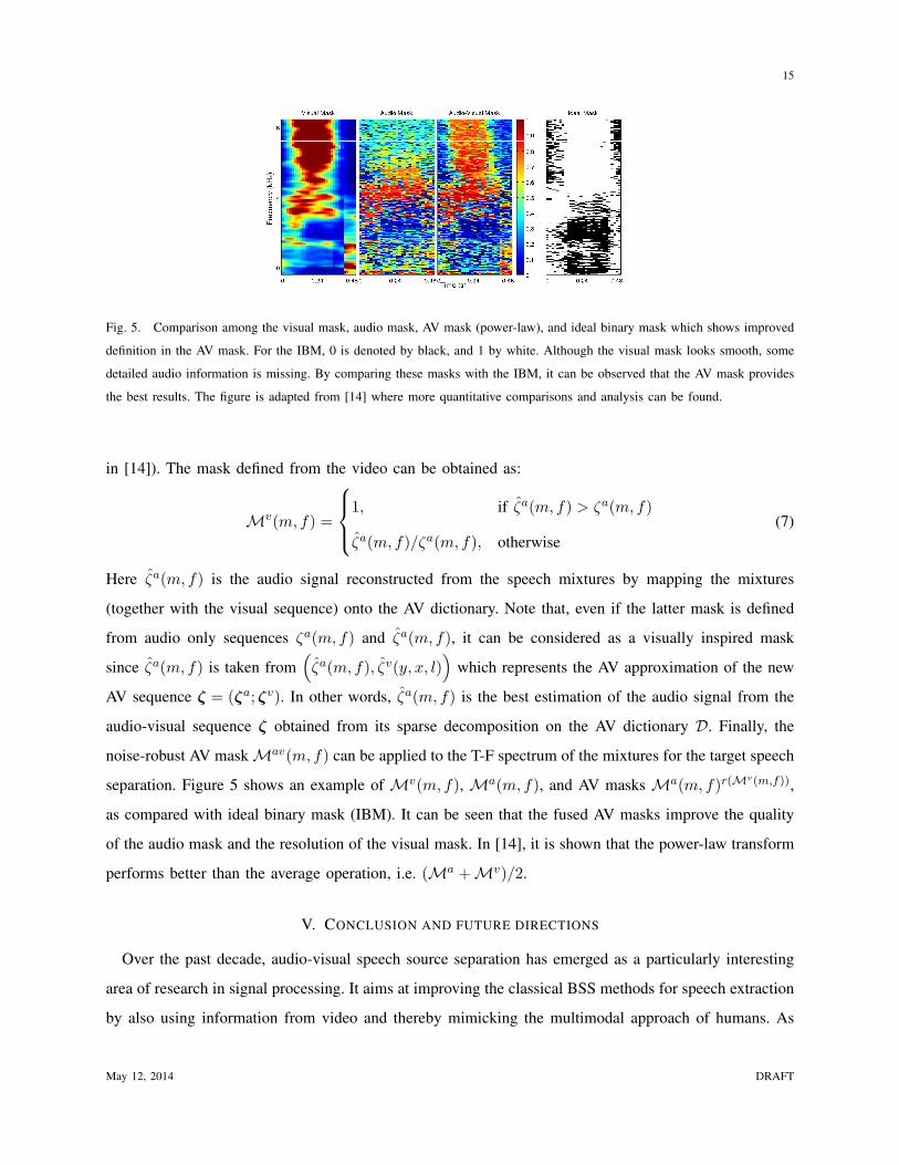
Fig. 5. Comparison among the visual mask, audio mask, AV mask (power-law), and ideal binary mask which shows improved
definition in the AV mask. For the IBM, 0 is denoted by black, and 1 by white. Although the visual mask looks smooth, some
detailed audio information is missing. By comparing these masks with the IBM, it can be observed that the AV mask provides
the best results. The figure is adapted from [14] where more quantitative comparisons and analysis can be found.
in [14]). The mask defined from the video can be obtained as:
Mv(m, f) =
1, if ζa(m, f) > ζa(m, f)
ζa(m, f)/ζa(m, f), otherwise
(7)
Here ζa(m, f) is the audio signal reconstructed from the speech mixtures by mapping the mixtures
(together with the visual sequence) onto the AV dictionary. Note that, even if the latter mask is defined
from audio only sequences ζa(m, f) and ζa(m, f), it can be considered as a visually inspired mask
since ζa(m, f) is taken from(
ζa(m, f), ζv(y, x, l))
which represents the AV approximation of the new
AV sequence ζ = (ζa; ζv). In other words, ζa(m, f) is the best estimation of the audio signal from the
audio-visual sequence ζ obtained from its sparse decomposition on the AV dictionary D. Finally, the
noise-robust AV mask Mav(m, f) can be applied to the T-F spectrum of the mixtures for the target speech
separation. Figure 5 shows an example of Mv(m, f), Ma(m, f), and AV masks Ma(m, f)r(Mv(m,f)),
as compared with ideal binary mask (IBM). It can be seen that the fused AV masks improve the quality
of the audio mask and the resolution of the visual mask. In [14], it is shown that the power-law transform
performs better than the average operation, i.e. (Ma +Mv)/2.
V. CONCLUSION AND FUTURE DIRECTIONS
Over the past decade, audio-visual speech source separation has emerged as a particularly interesting
area of research in signal processing. It aims at improving the classical BSS methods for speech extraction
by also using information from video and thereby mimicking the multimodal approach of humans. As
May 12, 2014 DRAFT

16
shown in this article, the bimodality of speech can be used at different levels of sophistication to help
audio source separation: from very coarse binary information through to a complete AV model, or from
simple joint lip shape parameters to data-dependent acoustic features represented in an AV dictionary.
As a result, the methods using the various level of information show different strength and weakness,
as highlighted in Table I. The main advantage of using the extra information from video is to tackle the
problems that cannot be easily solved by audio only algorithms, e.g., handling background noise and
interference in strongly reverberant environments, together with multiple, potentially moving, sources.
There are many directions for further research. The AV coherence based on statistical methods requires
high-quality low-dimensional features for accurate and computationally efficient modelling, therefore
emerging methods from manifold or deep learning could be exploited. The current methods in AV
dictionary learning which attempt to capture the AV informative structure in the bimodal data are
computationally expensive due to the intensive numerical operations required in sparse coding algorithms.
Low-complexity and robust algorithms are highly desirable and need to be developed. Moreover, to
be embedded in everyday devices such as smart phones, real time approaches must be proposed to
overcome the batch nature of many current algorithms. In the longer term, building richer models
exploiting psychoacoustic-visual properties on the basis of the fields of brain-science and psychology
can potentially further improve the AV speech separation systems, but this presents a particular challenge
for future research in this area.
Finally, as speech source separation is clearly profiting from the bimodality of sources, other fields of
source separation/extraction should also be explored using multimodal data, for instance brain imaging
which can record brain activity by electro-encephalography, magneto-encephalography, magnetic reso-
nance imaging and positron emission tomography. The next generation of intelligent multimodal signal
processing techniques will combine such information to provide radically improved performance not
achievable with methods based on single-modality data.
VI. ACKNOWLEDGEMENT
The authors thank the Guest Editors and the anonymous reviewers for their helpful comments to
drastically improve the quality of this paper. The authors thank Dr Qingju Liu for re-generating and
adapting Figures 4 and 5 which appeared originally in [14].
Part of this work was supported by the Engineering and Physical Sciences Research Council (EPSRC)
of the UK Grant number EP/J013644/1, the UK Ministry of Defence University Defence Research
Collaboration in Signal Processing and the European project ERC-2012-AdG-320684-CHESS.
May 12, 2014 DRAFT
17
REFERENCES
[1] P. Comon and C. Jutten, Eds., Handbook of Blind Source Separation Independent Component Analysis and Applications.
Academic Press, 2010.
[2] E. C. Cherry, “Some experiments on the recognition of speech, with one and with two ears,” Journal of Acoustical Society
of America, vol. 25, no. 5, pp. 975–979, 1953.
[3] A. P. Dempster, N. M. Laird, and D. B. Rubin, “Maximum-likelihood from incomplete data via the EM algorithm,” J.
Royal Statist. Soc. Ser. B., vol. 39, pp. 1–38, 1977.
[4] S. M. Naqvi, M. Yu, and J. A. Chambers, “A multimodal approach to blind source separation of moving sources,” IEEE
Journal of Selected Topics in Signal Processing, vol. 4, no. 5, pp. 895–910, 2010.
[5] L. E. Bernstein and C. Benoıt, “For speech perception by humans or machines, three senses are better than one,” in Proc.
Int. Conf. Spoken Language Processing (ICSLP), Philadelphia, USA, 1996, pp. 1477–1480.
[6] W. Sumby and I. Pollack, “Visual contribution to speech intelligibility in noise,” Journal of Acoustical Society of America,
vol. 26, pp. 212–215, 1954.
[7] A. Liew and S. Wang, Eds., Visual Speech Recognition: Lip Segmentation and Mapping. IGI Global Press, 2009.
[8] G. Potamianos, C. Neti, G. Gravier, A. Garg, and A. W. Senior, “Recent advances in the automatic recognition of audiovisual
speech,” Proceedings of the IEEE, vol. 91, no. 9, pp. 1306–1326, 2003.
[9] J.-L. Schwartz, F. Berthommier, and C. Savariaux, “Seeing to hear better: evidence for early audio-visual interactions in
speech identification,” Cognition, vol. 93, no. 2, pp. B69–B78, 2004.
[10] L. Girin, J.-L. Schwartz, and G. Feng, “Audio-visual enhancement of speech in noise,” Journal of Acoustical Society of
America, vol. 109, no. 6, pp. 3007–3020, June 2001.
[11] D. Sodoyer, J.-L. Schwartz, L. Girin, J. Klinkisch, and C. Jutten, “Separation of audio-visual speech sources: a new
approach exploiting the audiovisual coherence of speech stimuli,” EURASIP Journal on Applied Signal Processing, vol.
2002, no. 11, pp. 1165–1173, 2002.
[12] B. Rivet, L. Girin, and C. Jutten, “Mixing audiovisual speech processing and blind source separation for the extraction of
speech signals from convolutive mixtures,” IEEE Transactions on Audio, Speech and Language Processing, vol. 15, no. 1,
pp. 96–108, 2007.
[13] Q. Liu, W. Wang, and P. Jackson, “Use of bimodal coherence to resolve permutation problem in convolutive BSS,” Signal
Processing, vol. 92, no. 8, pp. 1916–1927, 2012.
[14] Q. Liu, W. Wang, P. Jackson, M. Barnard, J. Kittler, and J. Chambers, “Source separation of convolutive and noisy mixtures
using audio-visual dictionary learning and probabilistic time-frequency masking,” IEEE Transactions on Signal Processing,
vol. 61, no. 22, pp. 5520–5535, 2013.
[15] B. Rivet, L. Girin, C. Serviere, D.-T. Pham, and C. Jutten, “Using a visual voice activity detector to regularize the
permutations in blind source separation of convolutive speech mixtures,” in Proc. Int. Conf. on Digital Signal Processing
(DSP), Cardiff, Wales UK, July 2007, pp. 223–226.
[16] B. Rivet, L. Girin, and C. Jutten, “Visual voice activity detection as a help for speech source separation from convolutive
mixtures,” Speech Communication, vol. 49, no. 7-8, pp. 667–677, 2007.
[17] D. Sodoyer, B. Rivet, L. Girin, C. Savariaux, J.-L. Schwartz, and C. Jutten, “A study of lip movements during spontaneous
dialog and its application to voice activity detection,” Journal of Acoustical Society of America, vol. 125, no. 2, pp.
1184–1196, February 2009.
May 12, 2014 DRAFT

18
[18] A. L. Casanovas, G. Monaci, P. Vandergheynst, and R. Gribonval, “Blind audio-visual source separation based on sparse
redundant representations,” IEEE Transactions on Multimedia, vol. 12, no. 5, pp. 358–371, 2010.
[19] S. M. Naqvi, W. Wang, M. S. Khan, M. Barnard, and J. A. Chambers, “Multimodal (audio-visual) source separation
exploiting multi-speaker tracking, robust beamforming, and time-frequency masking,” IET Signal Processing, vol. 6, pp.
466–477, 2012.
[20] M. S. Khan, S. M. Naqvi, A. Rehman, W. Wang, and J. A. Chambers, “Video-aided model-based source separation in real
reverberant rooms,” IEEE Transactions on Audio, Speech and Language Processing, vol. 21, no. 9, pp. 1900–1912, 2013.
[21] Q. Liu and W. Wang, “Blind source separation and visual voice activity detection for target speech extraction,” in Proc.
International Conference on Awareness Science and Technology (iCAST), 2011, pp. 457–460.
[22] Q. Liu, A. Aubery, and W. Wang, “Interference reduction in reverberant speech separation with visual voice activity
detection,” IEEE Transactions on Multimedia, 2013, submitted.
[23] H. K. Maganti, D. Gatica-Perez, and I. McCowan, “Speech enhancement and recognition in meetings with an audio-visual
sensor array,” IEEE Transactions on Audio, Speech and Language Processing, vol. 15, no. 8, pp. 2257–2269, 2007.
[24] S. T. Shivappa, B. D. Rao, and M. M. Trivedi, “Audio-visual fusion and tracking with multilevel iterative decoding:
Framework and experimental evaluation,” IEEE Journal of Selected Topics in Signal Processing, vol. 4, no. 5, October
2010.
[25] Y. Liang, S. M. Naqvi, and J. A. Chambers, “Audio video based fast fixed-point independent vector analysis for multisource
separation in a room environment,” EURASIP Journal on Advances in Signal Processing, 2012:183.
[26] D. Sodoyer, L. Girin, C. Jutten, and J.-L. Schwartz, “Developing an audio-visual speech source separation algorithm,”
Speech Communication, vol. 44, no. 1–4, pp. 113–125, October 2004.
[27] W. Wang, D. Cosker, Y. Hicks, S. Sanei, and J. A. Chambers, “Video assisted speech source separation,” in Proc. IEEE
Int. Conf. Acoustics, Speech, and Signal Processing (ICASSP), Philadelphia, USA, March 2005.
[28] A. J. Aubrey, Y. A. Hicks, and J. A. Chambers, “Visual voice activity detection with optical flow,” IET Image Processing,
vol. 4, pp. 463–472, 2010.
[29] M. Anderson, G.-S. Fu, R. Phlypo, and T. Adali, “Independent vector analysis: Identification conditions and performance
bounds,” IEEE Transactions on Signal Processing, accepted for publication.
[30] A. Alinaghi, W. Wang, and P. J. B. Jackson, “Integrating binaural cues and blind source separation method for separating
reverberant speech mixtures,” in Proc. ICASSP, 2011, pp. 209–212.
[31] B. Rivet, L. Girin, and C. Jutten, “Log-Rayleigh distribution: a simple and efficient statistical representation of log-spectral
coefficients,” IEEE Transactions on Audio, Speech and Language Processing, vol. 15, no. 3, pp. 796–802, March 2007.
[32] G. Monaci, P. Vandergheynst, and F. T. Sommer, “Learning bimodal structure in audio-visual data,” IEEE Transactions on
Neural Networks, vol. 20, no. 12, pp. 1898–1910, 2009.
[33] B. Gold, N. Morgan, and D. Ellis, Speech and Audio Signal Processing - Processing and Perception of Speech and Music,
2nd ed. Wiley, 2011.
[34] T. Cootes, G. Edwards, and C. Taylor, “Active appearance models,” IEEE Transactions on Pattern Analysis and Machine
Intelligence, vol. 23, no. 6, pp. 681–685, 2001.
[35] M. Aharon, M. Elad, and A. Bruckstein, “K-SVD: An algorithm for designing overcomplete dictionaries for sparse
representation,” IEEE Transactions on Signal Processing, vol. 54, no. 11, pp. 4311–4322, 2006.
[36] M. I. Mandel, R. J. Weiss, and D. Ellis, “Model-based expectation-maximization source separation and localization,” IEEE
Transactions on Audio, Speech and Language Processing, vol. 18, no. 2, pp. 382–394, 2010.
May 12, 2014 DRAFT