AudioQuilt: 2D Arrangements of Audio Samples usingMetric Learning and Kernelized Sorting

Ohad FriedPrinceton University

ohad@cs.princeton.edu

Zeyu JinPrinceton University

zjin@cs.princeton.edu

Reid OdaPrinceton University

roda@cs.princeton.edu

Adam FinkelsteinPrinceton Universityaf@cs.princeton.edu

ABSTRACTThe modern musician enjoys access to a staggering num-ber of audio samples. Composition software can ship withmany gigabytes of data, and there are many more to befound online. However, conventional methods for navigat-ing these libraries are still quite rudimentary, and often in-volve scrolling through alphabetical lists. We present Au-dioQuilt, a system for sample exploration that allows audioclips to be sorted according to user taste, and arranged inany desired 2D formation such that similar samples are lo-cated near each other. Our method relies on two advancesin machine learning. First, metric learning allows the userto shape the audio feature space to match their own prefer-ences. Second, kernelized sorting finds an optimal arrange-ment for the samples in 2D. We demonstrate our systemwith three new interfaces for exploring audio samples, andevaluate the technology qualitatively and quantitatively viaa pair of user studies.

KeywordsSound Exploration, Sample Library, Metric Learning, Ker-nelized Sorting

1. INTRODUCTIONThe age of “big data” has brought upheaval in many as-pects of our lives including photography, retail, social net-works and music. The modern musician or composer hasat her disposal a vast array of sound samples, and acquir-ing more requires little effort. Once the acquisition processbecomes easy, the burden passes to the next stage, whichis managing, searching, and exploring this data. A hugeaudio database is rendered nearly useless if it is impossibleto navigate and find a desired clip.

Proper organization of audio samples is a challengingproblem because similarity between samples is largely sub-jective. Audio features that are important to one user maybe less important to others. Additionally, it’s unclear howa sorted collection should be arranged on a computer screenin order to make best use of the space, and to maximize thebrowsing experience. In this paper we offer two techniquesto address these problems. First, metric learning (Section3.1) allows users to specify their own groupings of samples.

Permission to make digital or hard copies of all or part of this work forpersonal or classroom use is granted without fee provided that copies arenot made or distributed for profit or commercial advantage and that copiesbear this notice and the full citation on the first page. To copy otherwise, torepublish, to post on servers or to redistribute to lists, requires prior specificpermission and/or a fee.NIME’14, June 30 – July 03, 2014, Goldsmiths, University of London, UK.Copyright remains with the author(s).

The system then learns which features are important, byupweighting those which are most useful for classification,and ignoring those that are not important, and can thenapply these weightings to new, as of yet unseen, samples.Next, we use kernelized sorting [18] (Section 3.2) in orderto place samples onto target locations on a 2D plane, suchthat similar samples are near each other. This means thatthe samples can be arranged in any arbitrary pattern, suchas a grid, a circle, a line, or a cluster. Kernelized sort-ing places the samples on the targets locations in a mannerthat respects the distances learned by metric learning. Thisapproach provides particular flexibility when working withinterfaces where real estate is scarce, or when building tan-gible controllers that have discrete buttons.

Our main contributions are (1) using metric learning totransform descriptors into a better space via user guidanceand (2) using kernelized sorting to place the samples in aspecific arrangement. While both techniques are known inother fields, their combination and usage for sound explo-ration is novel. Finally, we demonstrate two novel interfacesfor audio navigation supported by our approach, and evalu-ate it both qualitatively and quantitatively via user studies.

2. BACKGROUNDIn this section we discuss previous work and establishedmethods for sound exploration and layout. We also providebackground regarding metric learning and set matching, thetwo main components of our approach.

2.1 Sound Exploration and LayoutSorting samples by timbral similarity, and visualizing themin a 2D plane is a well-studied field [9]. The process usu-ally involves three steps. The first step is feature extrac-tion. Commonly used features include bark-scale coeffi-cients [15, 6], MPEG-7 [20, 15], and mel-frequency cepstralcoefficients [8, 3]. Bark scale and mel-frequency cepstralcoeffients are representations of the spectral envelope, com-pressed to smaller dimensionality, while MPEG-7 includesfeatures which are relevant to perception of timbre [17].

Next, the similarity between each sample is expressed.Common approaches include embedding the sample in multi-dimensional space and expressing the similarity as a dis-tance such as euclidean [7, 8], generalized minkowski[16],mahalanobis [8, 20]. Sometimes the dimensions are reducedusing PCA, multi-dimensional scaling [7] or similar.

Finally, the samples are represented in a 2D plane. Themost popular approach is to use self-organizing maps [4,6, 23, 24]. Our chosen method for embedding, kernelizedsorting [18], differs from self-organizing maps in that it al-lows us to specify where the samples should be placed, andachieves a 1-to-1 mapping between sound samples and tar-

Figure 1: We produce a 1-to-1 matching betweensound samples and grid locations (left), while meth-ods such as Self Organizing Maps can match severalor no samples to the same node (right).

get locations (i.e. all target locations are filled). This allowsus to place the samples on dense structures such as grids.In comparison, in the training phase, self-organizing mapscreate a map by assigning values to a set of nodes (neu-rons), and in the mapping phase each element is mappedto its closest node. This means that many samples can bemapped to the same node, and some nodes might remainvacant (Figure 1).

2.2 Metric LearningEmbedding high dimensional features to 2D grid relies heav-ily on the measurement of similarity or distance. Many ma-chine learning techniques such as K-means and KNN assumeEuclidean space and L2 distance, where the dimensions areassumed to be independent and equally important. How-ever, the Euclidean assumption is often not true. Whenmeasuring the similarities of snare drums samples based onspectrum and envelope features, the interactions betweenspectral dimensions and the difference scaling factors be-tween the spectrum (energy) and the envelope (time) makethe space non-Euclidean. Furthermore, when it comes toaudio exploration, different users have different perceptionsof the similarity. Metric learning properly adjusts the fea-ture space to be Euclidean.

There are two types of metric learning, supervised andunsupervised. The unsupervised metric learning methodtransforms a vector x by a matrix M such that the elementsin Mx are independent and normalized. Principal Compo-nent Analysis (PCA) and Multidimensional Scaling (MDS)both fall into this category. The main difference betweenthe two is that PCA preserves the data variance while MDSpreserves the inter-point distance [28]. However, unsuper-vised metric learning does not find the best presentationwhen the data is sampled from multiple subspace clusters.That is why we refine the feature space based on supervisedmetric learning.

Supervised metric learning requires that the data is la-beled with pairwise constraints of either“similar”or“dissim-ilar.” The simplest supervised metric learning method is lin-ear discriminative analysis (LDA), which uses class labels tomaximally separate two classes of data [12]. A more sophis-ticated method is devised by Xing et al. [26] for Mahalanobisdistance metric [14]. It finds a new metric M , such that the

new distance measure d(x, y) =√

(x− y)TM(x− y) min-imizes the distance of similar samples, and preserves thedistances of dissimilar samples. For multiple data clusters(especially in the context of audio sample browsing) we ex-tend this learning scheme to group-based constraints wherewe maximize the between-group distance, while preservingthe upper-bound of the in-group distance.

2.3 Set MatchingPicking the best locations for audio samples can be formu-lated as a set matching problem, where the first set cor-responds to the audio samples and the second to the 2D

locations. Given two sets for which intra-set distances areknown (but not inter-set distances), the problem of findinga permutation that best matches the two sets can be formu-lated as a Quadratic Assignment Problem (QAP) [11]. SinceQAP is NP-Hard, an exact solution is generally out of reachand approximations or relaxations should be pursued. Suchrelaxations include kernelized sorting (KS) [18] and convexkernelized sorting (CKS) [5], both of which we use as partof our algorithm. Other options include KS-NOCCO andLSOM [27]. We choose KS due to its simplicity and speed,and find the performance to be adequate. We also imple-ment CKS, which generally gives improved quality but atthe cost of noticeably slower performance for large arrange-ments. (Future work might quantize the just-noticeable-differences and/or quantitatively compare different sortingapproaches.) It is important to note that any of these meth-ods can be used interchangeably in our algorithm, as we donot rely on any specific implementation details.

3. ALGORITHMOur algorithm is formed as a two-part process, in which weaim to (1) automatically learn the correct relationships be-tween sound samples based on user preferences and (2) au-tomatically place the sound samples in a predefined arrange-ment that respects the previously learned relationships. Weachieve these two tasks by using metric learning and kernel-ized sorting, respectively. In this section we describe thesetechniques and how we build on them in AudioQuilt.

3.1 Learning Correct RelationshipsMetric learning allows us to incorporate user-supplied group-ings of data. In the standard formulation, we suppose weobserve a set of points {xi}1:m ⊆ Rn and are given thegrouping information {yi}1:m ⊆ {1, 2, ...,K}n where yi isthe group label of point xi. The supervised Mahalanobismetric learning problem is to learn the new distance met-ric ‖x − y‖A ≡ dA(x, y) =

√(x− y)TA(x− y), such that

the pairwise distances of the points in the same group arekept small, while the distances of points between differentgroups are maximized. Note that the matrix A needs tobe semi-definite such that the triangle property is satis-fied for the new metric. Because

√(x− y)TA(x− y) =√

(x− y)TBTB(x− y) where B = A1/2, this method es-sentially finds a new space Bx for vector x. According toXing et al. [26], a plausible formulation for multiple groupmetric learning can be:

maxA

∑(i,j)|yi 6=yj

‖xi − xj‖A (1)

s.t.∑

(i,j)|yi=yj=k

‖xi − xj‖2A ≤ 1 for k ∈ [K], A � 0

Note that the objective is the sum of distances, and notthe sum of squared distances, so semi-definite programmingcannot be utilized. We do not want to change the objectiveto the sum of squared distances, because it leads to a rank-one solution of A, where all the data points are aligned ontoa line [26]. But because of the convexity of this formula, wecan still obtain the global maximum using gradient descentand iterative projection. However, the optimization is slow,which is unsuitable for a real-time application. To boost thespeed and avoid low-rank solution, we propose the followingoptimization scheme for the metric learning:

maxA

∑(i,j)|yi 6=yj

‖xi − xj‖2A − λ∑

(i,j)|yi=yj

‖xi − xj‖2A (2)

s.t. ‖xi − xj‖2A ≤ 1 (i, j) ∈ {(i, j)|yi = yj}, A � 0

where the term λ is the weight of in-group distance penalty.Increasing this term yields more concentrated groups, whichare closer to one another. In this work, we set this value to1, meaning both in-group concentration and between-groupdivergence are important.

The new formula can be optimized using semi-definiteprogramming and thus much faster to compute comparedto the previous method.

3.2 Location AssignmentThe inputs to the location assignment part of our algorithmare pairwise distances between n sound samples (i.e. dij isthe distance between sound sample i and sound sample j,dii = 0) and target locations. Target locations P is an arbi-trary set of 2D (or 3D) points in Euclidean space, such that|P| = n. The goal is to find a bijection between the soundsamples and the locations, such that pairwise distances arepreserved as much as possible. Intuitively, we would likefor similar sound samples to be placed close together andfor dissimilar samples to be far apart. We achieve this goalby using two previously established algorithms: kernelizedsorting [18] and convex kernelized sorting [5].kernelized sorting. While we aim to solve a specific

problem of matching sound samples to target locations, ker-nelized sorting is a general method to match any two equallysized sets, given an intra-set similarity measure (but notinter-set). More formally, we are given two setsX = {xi}ni=1

and Y = {yi}ni=1, which may belong to two different do-mains X and Y. We are also given two kernel functionsk : X × X → R and l : Y × Y → R which indicate thesimilarity between objects of X and Y respectively (i.e. alarge value of k(xi, xj) indicates that xi and xj are sim-ilar). We can represent the kernel values of our data inmatrix notation as K and L, where Kij = k(xi, xj) andLij = l(yi, yj) (we borrow the same notation as in KS [18]).Let us mark K and L as the centralized versions of K andL. The goal of KS is to find a permutation matrix Π suchthat K and ΠTLΠ are similar. The similarity criteria usedis the Hilbert-Schmidt Independence Criterion [21]. An it-erative approach is used to maximize an approximation ofthat criteria. We refer the reader to [18] for more details.

In our case, X are sound samples and Y are 2D locationsas specified by the user. We compute similarity betweensound samples by the Euclidean distance of the adjustedfeature space learned from supervised metric learning. Thesimilarity between two locations is the reciprocal of the Eu-clidean distance between them. KS allows us to interac-tively assign sound samples to user-specified locations.Convex Kernelized Sorting Over the years several im-

provements to kernelized sorting have be proposed. Onesuch method is convex kernelized sorting (CKS) [5]. Theobjective function is changed so that the problem becomesa convex minimization problem, as shown in Equation 3.We use Π, K and L as before, and ‖ · ‖F denotes the Frobe-nius norm.

minΠ‖K ·ΠT − (L ·Π)T ‖2F (3)

The authors of CKS [5] show that the new method achievesbetter results in tasks such as image matching. The im-proved performance comes at a cost of a slower algorithm,due to a non-linear optimization step. We have incorporatedCKS into our system and can dynamically pick between KSand CKS, achieving a performance-vs-runtime balance.

It is important to note that while we had good reasons tochoose these specific algorithms (as explained above), theycan be easily swapped in and out. Any other algorithm thatcan create a bijection from a distance measure is suitable

for our needs, and the rest of the pipeline does not dependon the specific implementation.

4. APPLICATIONSIn this section we present 3 interfaces that we prototypedusing our system. We demonstrate applications for soundsample navigation, as well as audio synthesis.

4.1 Snare-Drum NavigatorMuch like fabric for the clothes designer and wood for thecarpenter, sound samples are essential building material forthe modern day music composer. It is not unusual for anartist to collect hundreds and thousands of sound snippets,ranging diverse categories. All those samples are, at best,arranged by category (e.g. electric guitar, tires screeching,female vocals) and at worst just dumped into a single folderand sorted alphabetically according to file name. Despitea number of viable sample exploration systems [8, 25, 2,19] developed by researchers in past years, it appears thatcommercial composition tools are only just now beginningto implement a“more like this”feature for sound samples [1],and we feel the interface can go even further.

Our snare drum navigator is simple to describe: the useris presented with a 2D grid of rectangles, each with a slightlydifferent color. Proximity of rectangles implies similar soundqualities. The color can either emphasize similarity, or beused as a channel to convey an extra layer of information. Inthis application we applied two coloring scheme. The firstone is generated by Isomap [22] which projects the originalfeatures (24-D) to 2D and use them as the first two channelsin LAB color space (the thrid channel is fixed in this case).The second scheme is to apply k-means to find clusters, thenuse the 3 principal components of the features to create aninitial coloring based LAB space, and finally move the colorof each sample towards the center of its assigned cluster.The corresponding waveform is displayed inside each rect-angle. Following feedback from early users, we also showthe history of the exploration process by fading out visitedcells and fading them back in over time.

The feature vector for this application is constructed asfollows. First the samples are normalized; the onset timeis detected and aligned via a threshold of -30dB. Next weuse MIRtoolbox [13] to obtain the envelope and the logattack time; we compute the temporal centroid and two 11-coefficient MFCCs of window size 2048 at the onset and

Figure 2: Snare drum navigator. The user is pre-sented with a grid of colored rectangles, each corre-sponds to a sound sample. Hovering over samplesproduces sound; similar sounds are placed in prox-imity. The feature vector consists of MFCC descrip-tors, log attack time and temporal centroids. Wesupport several coloring schemes, either accordingto the features used or according to other informa-tion we wish to convey. Here we show Isomap col-oration (left) and k-means based coloring (right).

Figure 3: Our interface for metric adjustment. Eachcircle corresponds to a sound sample. The user canhover over samples to play them. Circles are colorcoded by the user according to their group by click-ing (groups are shown at the bottom). Pressing“Compute Assignment” triggers a calculation of anew metric such that the user supplied labeling isrespected. This GUI allows for interactive manipu-lation of the distance metric according to the user’sneeds, which can be applied to create new soundlayouts (Figure 2).

after the attack (sustain). We concatenate these three at-tributes (24 dimensions in total) as the feature descriptor.

Figure 2 shows our snare drum navigator. We first learnedthe metric space using a training set of snares, manually la-beling 176 samples out of a total of 839 in the training setinto 12 categories. We note that this is a one time processfor each data type (i.e. we can now sort snares withoutrepeating this process). The total labeling time was about30 minutes. We then applied the metric to the displayedtest set. The result is an arrangement with different typesof snares clustered in different parts of the interface. In theupper left are aggressive, punchy snares, while in the lowerright are thin, snappy snares. In between there is a gra-dient of snare types ranging (moving top to bottom) fromhip-hop vinyl snares, to woody acoustic snares, to thin andlight acoustic snares. We refer the user to the accompany-ing video for a more audible experience. We also show thesame sound layout, with a different color scheme.

We also allow the user to interactively adjust the learnedmetric by assigning group labels to examplars. Figure 3shows the interface. Starting from a layout, a user can lis-ten to the samples and indicate the proper group by chang-ing the colors of the nodes. Then he/she presses “compute”and the system uses the grouping information to learn a newmetric that enlarges the difference between different colors,and then apply it to the distance matrix for kernelized sort-ing to obtain a new layout.

4.2 Synth ExplorerWe can also use our method to explore audio synthesizerparameters. The task of navigating synthesizer parameterscan be challenging due to the diverse sounds and the nonlin-ear ways in which parameters interact. Furthermore, manynovice users do not understand all the different buttons andknobs that are present on a synth. We aim to alleviate theproblem by supplying an intuitive interface for exploringsynth parameters and the resulting sounds.

In this system we use a simple synthesizer with 4 param-eters: Pitch, FM amount, FM frequency, and Ring modula-tion frequency. The features used are MFCCs with a 8000sample window and the log attack time.

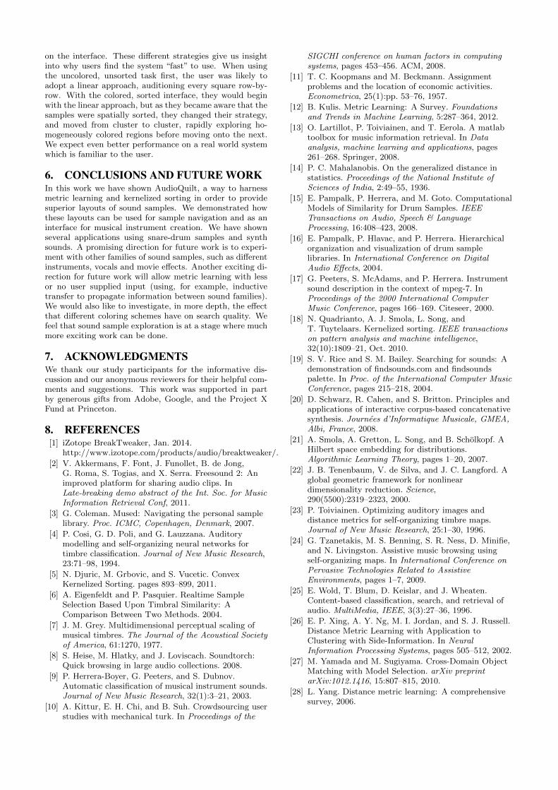
The interface is shown in figure 4. Each node represents asound created by a given synth parameter setting. To begin,

Figure 4: Synth sound explorer. Synthesizer pa-rameters are sampled to create sound snippets andarranged by sound similarity. The user hovers overthe circles to listen to the snippets, and can indicatelikes/dislikes. The space is re-sampled and re-sortedinteractively according to the user’s selection. Werefer the reader to the accompanying video for amore vivid demonstration.

we sample uniformly at random, from the parameter spaceof the synthesizer. For each parameter setting we record a1-second sound clip, and use kernelized sorting to map itonto a node, so that timbrally similar sounds are near oneanother. Mousing over a node plays the sound. The layoutof nodes is freely configurable. If the nodes are moved (theuser can drag the circles), the sound-to-node mapping is re-computed to maintain the timbral relationships. The userthen indicates which sounds they like, and some that theydon’t like. These two labels are used as classes for met-ric learning to recompute the space. Once the space hasbeen recomputed, the system samples around the parame-ter space of each “liked” setting. This creates a hierarchicalmethod for exploring the space. The new samples are ar-ranged in the same manner described earlier. Note thatsounds with very different parameters, but similar timbres,will be arranged next to one another, enabling the user tosearch by audio, not parameter. When they want to learnthe parameters, they click the node, and the parameters ofthe synth are shown on the right side of the screen. Theycan also search by adjusting the parameters directly.

5. USER STUDIESWe evaluated our system using two methods – one in-personand the other online. The in-person study aims to get qual-itative feedback from musicians on the usability of the sys-tem, while the online study was geared towards quantitativeresults, to help us understand which aspects of the systemaffected search time and accuracy. Both studies used thesnare drum navigator shown in Figure 2.

5.1 In-Person Qualitative StudyOur in-person study involved 5 musicians. Each of themwere familiar with composition using a DAW, and the pro-cess of sample selection. They ranged from 20-33 years inage and consisted of 2 undergraduate students, 2 graduatestudents and one faculty member.

We adopted a contextual observation style approach, giv-ing the user only basic instructions and offering informationonly when asked. Before the user study, we pre-trained thesystem using metric learning. The users were instructed touse the system as if they were browsing for snare drumsfor a project. As they browsed they narrated their experi-ence. After they had located a few snares that they liked,

we conducted a semi-structured interview.The most common feedback we received is that the sys-

tem was very “fast”. People liked the ability to auditiona number of samples very rapidly. All of the users spon-taneously identified clusters of similar snares in the inter-face. Some comments included “these here have scoopedout mids” and “here are a bunch of hip-hop vinyl samples”.However, they were sometimes surprised by certain snaresthat seemed not to fit their neighbors at all, “this snareshould be over there”, was a common comment. These un-expected snares appeared to diminish the user’s confidencein their understanding of the system.

5.2 Online Quantitative StudyThe goal of our second studyis to evaluate our systemquantitatively by testing aperson’s ability to find par-ticular sounds among a col-lection. In a typical com-position situation an artistmight not be looking for aspecific sound among theircollection, just one that is“close enough.” For each test, we generated 10 “closeenough” sounds, which are similar to an exemplar sound,and 90 samples that are dissimilar. The goal of the task isto find as many of the 10 “close” samples as possible within60 seconds. To create samples, we first randomly generate2000 synthesized samples; then we extract the audio fea-tures and compute k-means to obtain 10 clusters; finally,we pick sample around the cluster centers.

In the study, subjects were presented with our grid inter-face as well as the reference exemplar sound (shown inset).Before the test began, each subject read a short explana-tion of the task. Then they were allowed to listen to theexemplar as many times as they liked. Once they beganbrowsing the grid of samples, they were given 60 seconds tomark up to 10 similar sounds. To mark a sound as similar,they clicked on the rectangle and a check mark appeared;an optional subsequent click would remove the mark. Ifsubjects were satisfied with their selection, they could endthe task early.

In our test, the independent variables were: (1) grid color-ing enabled or disabled, crossed with: (2) Kernelized Sort-ing versus random arrangement. This yielded 4 differentconditions. Each condition was paired with a different sam-ple set (selected randomly from among 8 total sets) and ev-ery subject was presented with all four conditions in randomorder. We recruited 100 subjects using the Amazon Me-chanical Turk (a microtask marketplace shown to be effec-tive for online user studies [10]). Each subject spent approx-imately 5 minutes completing one “human intelligence task”(HIT). Each subject was randomly assigned a set-conditionpair, and did exactly one HIT. In total we collected datafrom 100 HITs, and thus our experiments include a total of400 trials (100 in each condition).

The 400 trials are plotted in Figure 5 as the correct num-ber of marked samples vs. time. Notice there is a distinctshape to the spatially sorted trials: the subject tends tomake little progress for a while, then the number of correctanswers skyrockets. We hypothesize that this is the momentwhen the proper cluster is found. In contrast, the unsortedtrials show a slower progress towards the maximum, withno great leaps. Overall, the bird’s eye view is that the bestperforming condition (quickest to achieve high numbers ofcorrect answers) is the use of sorted arrangements togetherwith color.

0 10 20 30 40 50 600

1

2

3

4

5

6

7

8

9

10

Time (secs)

Co

rre

ct

An

sw

ers

0 10 20 30 40 50 600

1

2

3

4

5

6

7

8

9

10

Time (secs)

Co

rre

ct

An

sw

ers

(a) not sorted, no color (b) not sorted, color

0 10 20 30 40 50 600

1

2

3

4

5

6

7

8

9

10

Time (secs)

Corr

ect A

nsw

ers

0 10 20 30 40 50 600

1

2

3

4

5

6

7

8

9

10

Time (secs)

Corr

ect A

nsw

ers

(c) sorted, no color (d) sorted, color

Figure 5: Individual and aggregate results from theonline user study. Each thin lines is the perfor-mance of a single user in the 60 second trial, Y-axisis number of correct answers. Wide dashed line in-dicates mean over all 100 trials; wide solid indicatesmedian. Steeper is better, and in aggregate thesorted arrangement with color (d) is best.

0 10 20 30 40 50 6010

−5

10−4

10−3

10−2

10−1

100

time (seconds)

p−

va

lue

s

sorted (fig5:ab−cd)

color (fig5:ac−bd)

+color (fig5:c−d)

+sorted (fig5:b−d)

p=0.05

0 10 20 30 40 50 6010

−8

10−6

10−4

10−2

100

time (seconds)

p−

va

lue

s

sorted (fig5:ab−cd)

color (fig5:ac−bd)

+color (fig5:c−d)

+sorted (fig5:b−d)

p=0.05

(a) 100 users, 100 HITs (b) 45 Users, 100 HITs

Figure 6: P-value plots against time. Four ANOVAtests are shown; the response variable is the num-ber of correct answers at time t. Tests are “sorted”:sorted versus unsorted; “color”: color versus nocolor; “+color”: sorted with versus without color;“+sorted”: colored with versus without sorting.Legend labels also refer to Figure 5. Left: 100unique users. Right: 45 users, each allowed to re-peat the HIT up to 5 times (100 HITs in total).

We also evaluate these trajectories numerically. Our de-pendent variable is the number of correct answers at time t.We constructed 4 tests and evaluated their p-values every 2seconds. The results can be seen in Figure 6(a). The datashows that spatial sorting has significant effects early on (p-value < 10−3 at around 20 seconds). Spatial sorting alsohas an effect when only considering colored data (p-value≈ 10−3 in the 30–40 second time-frame). The U-shape ofthe curves hints that given enough time, all conditions willconverge (since the user can inspect all samples when timeis abundant). Color is mostly insignificant. We hypothesizethat our users did not have a chance to learn the meaning ofcolor. Thus, in another experiment (Figure 6(b)) we allowthe same user to perform several HITs (45 users, 100 HITs),in which case color becomes significant. In both versions ofthe experiment, arrangement was the most important factorin user success.

We logged all the events in the study, so we were ableto see exactly how a subject interacted with the system.We found that people used different strategies depending

on the interface. These different strategies give us insightinto why users find the system “fast” to use. When usingthe uncolored, unsorted task first, the user was likely toadopt a linear approach, auditioning every square row-by-row. With the colored, sorted interface, they would beginwith the linear approach, but as they became aware that thesamples were spatially sorted, they changed their strategy,and moved from cluster to cluster, rapidly exploring ho-mogeneously colored regions before moving onto the next.We expect even better performance on a real world systemwhich is familiar to the user.

6. CONCLUSIONS AND FUTURE WORKIn this work we have shown AudioQuilt, a way to harnessmetric learning and kernelized sorting in order to providesuperior layouts of sound samples. We demonstrated howthese layouts can be used for sample navigation and as aninterface for musical instrument creation. We have shownseveral applications using snare-drum samples and synthsounds. A promising direction for future work is to experi-ment with other families of sound samples, such as differentinstruments, vocals and movie effects. Another exciting di-rection for future work will allow metric learning with lessor no user supplied input (using, for example, inductivetransfer to propagate information between sound families).We would also like to investigate, in more depth, the effectthat different coloring schemes have on search quality. Wefeel that sound sample exploration is at a stage where muchmore exciting work can be done.

7. ACKNOWLEDGMENTSWe thank our study participants for the informative dis-cussion and our anonymous reviewers for their helpful com-ments and suggestions. This work was supported in partby generous gifts from Adobe, Google, and the Project XFund at Princeton.

8. REFERENCES[1] iZotope BreakTweaker, Jan. 2014.

http://www.izotope.com/products/audio/breaktweaker/.

[2] V. Akkermans, F. Font, J. Funollet, B. de Jong,G. Roma, S. Togias, and X. Serra. Freesound 2: Animproved platform for sharing audio clips. InLate-breaking demo abstract of the Int. Soc. for MusicInformation Retrieval Conf, 2011.

[3] G. Coleman. Mused: Navigating the personal samplelibrary. Proc. ICMC, Copenhagen, Denmark, 2007.

[4] P. Cosi, G. D. Poli, and G. Lauzzana. Auditorymodelling and self-organizing neural networks fortimbre classification. Journal of New Music Research,23:71–98, 1994.

[5] N. Djuric, M. Grbovic, and S. Vucetic. ConvexKernelized Sorting. pages 893–899, 2011.

[6] A. Eigenfeldt and P. Pasquier. Realtime SampleSelection Based Upon Timbral Similarity: AComparison Between Two Methods. 2004.

[7] J. M. Grey. Multidimensional perceptual scaling ofmusical timbres. The Journal of the Acoustical Societyof America, 61:1270, 1977.

[8] S. Heise, M. Hlatky, and J. Loviscach. Soundtorch:Quick browsing in large audio collections. 2008.

[9] P. Herrera-Boyer, G. Peeters, and S. Dubnov.Automatic classification of musical instrument sounds.Journal of New Music Research, 32(1):3–21, 2003.

[10] A. Kittur, E. H. Chi, and B. Suh. Crowdsourcing userstudies with mechanical turk. In Proceedings of the

SIGCHI conference on human factors in computingsystems, pages 453–456. ACM, 2008.

[11] T. C. Koopmans and M. Beckmann. Assignmentproblems and the location of economic activities.Econometrica, 25(1):pp. 53–76, 1957.

[12] B. Kulis. Metric Learning: A Survey. Foundationsand Trends in Machine Learning, 5:287–364, 2012.

[13] O. Lartillot, P. Toiviainen, and T. Eerola. A matlabtoolbox for music information retrieval. In Dataanalysis, machine learning and applications, pages261–268. Springer, 2008.

[14] P. C. Mahalanobis. On the generalized distance instatistics. Proceedings of the National Institute ofSciences of India, 2:49–55, 1936.

[15] E. Pampalk, P. Herrera, and M. Goto. ComputationalModels of Similarity for Drum Samples. IEEETransactions on Audio, Speech & LanguageProcessing, 16:408–423, 2008.

[16] E. Pampalk, P. Hlavac, and P. Herrera. Hierarchicalorganization and visualization of drum samplelibraries. In International Conference on DigitalAudio Effects, 2004.

[17] G. Peeters, S. McAdams, and P. Herrera. Instrumentsound description in the context of mpeg-7. InProceedings of the 2000 International ComputerMusic Conference, pages 166–169. Citeseer, 2000.

[18] N. Quadrianto, A. J. Smola, L. Song, andT. Tuytelaars. Kernelized sorting. IEEE transactionson pattern analysis and machine intelligence,32(10):1809–21, Oct. 2010.

[19] S. V. Rice and S. M. Bailey. Searching for sounds: Ademonstration of findsounds.com and findsoundspalette. In Proc. of the International Computer MusicConference, pages 215–218, 2004.

[20] D. Schwarz, R. Cahen, and S. Britton. Principles andapplications of interactive corpus-based concatenativesynthesis. Journees d’Informatique Musicale, GMEA,Albi, France, 2008.

[21] A. Smola, A. Gretton, L. Song, and B. Scholkopf. AHilbert space embedding for distributions.Algorithmic Learning Theory, pages 1–20, 2007.

[22] J. B. Tenenbaum, V. de Silva, and J. C. Langford. Aglobal geometric framework for nonlineardimensionality reduction. Science,290(5500):2319–2323, 2000.

[23] P. Toiviainen. Optimizing auditory images anddistance metrics for self-organizing timbre maps.Journal of New Music Research, 25:1–30, 1996.

[24] G. Tzanetakis, M. S. Benning, S. R. Ness, D. Minifie,and N. Livingston. Assistive music browsing usingself-organizing maps. In International Conference onPervasive Technologies Related to AssistiveEnvironments, pages 1–7, 2009.

[25] E. Wold, T. Blum, D. Keislar, and J. Wheaten.Content-based classification, search, and retrieval ofaudio. MultiMedia, IEEE, 3(3):27–36, 1996.

[26] E. P. Xing, A. Y. Ng, M. I. Jordan, and S. J. Russell.Distance Metric Learning with Application toClustering with Side-Information. In NeuralInformation Processing Systems, pages 505–512, 2002.

[27] M. Yamada and M. Sugiyama. Cross-Domain ObjectMatching with Model Selection. arXiv preprintarXiv:1012.1416, 15:807–815, 2010.

[28] L. Yang. Distance metric learning: A comprehensivesurvey, 2006.