Audio Features & Parametric Representations Machine...
18
1 API2011 Audio Features & Machine Learning E.M. Bakker API2011 Features for Speech Recognition and Audio Indexing Parametric Representations – Short Time Energy – Zero Crossing Rates – Level Crossing Rates – Short Time Spectral Envelope Spectral Analysis – Filter Design – Filter Bank Spectral Analysis Model – Linear Predictive Coding (LPC) API2011 Methods Vector Quantization – Finite code book of spectral shapes – The code book codes for ‗typical‘ spectral shape – Method for all spectral representations (e.g. Filter Banks, LPC, ZCR, etc. …) Support Vector Machines Markov Models Hidden Markov Models Neural Networks Etc. API2011 Pattern Recognition Reference Patterns Parameter Measurements Decision Rules Pattern Comparison Speech Audio, … Recognized Speech, Audio, … Test Pattern Query Pattern
Transcript of Audio Features & Parametric Representations Machine...

1
API2011
Audio Features &
Machine Learning
E.M. Bakker
API2011
Features for Speech Recognition
and Audio Indexing
Parametric Representations
– Short Time Energy
– Zero Crossing Rates
– Level Crossing Rates
– Short Time Spectral Envelope
Spectral Analysis
– Filter Design
– Filter Bank Spectral Analysis Model
– Linear Predictive Coding (LPC)
API2011
Methods
Vector Quantization
– Finite code book of spectral shapes
– The code book codes for ‗typical‘ spectral shape
– Method for all spectral representations (e.g. Filter
Banks, LPC, ZCR, etc. …)
Support Vector Machines
Markov Models
Hidden Markov Models
Neural Networks Etc.
API2011
Pattern Recognition
Reference
Patterns
Parameter
Measurements
Decision
Rules
Pattern
Comparison
Speech
Audio, …
Recognized
Speech, Audio, …
Test Pattern
Query Pattern

2
API2011
Pattern Recognition
Reference
Vocabulary
Features
Feature Detector1
Hypothesis
Tester
Feature Combiner
and
Decision Logic
Speech
Audio, …
Recognized
Speech, Audio, …
Feature Detectorn
API2011
Vector Quantization
Data represented as feature vectors.
VQ Training set to determine a set of code
words that constitute a code book.
Code words are centroids using a similarity or
distance measure d.
Code words together with d divide the space into
a Voronoi regions.
A query vector falls into a Voronoi region and will
be represented by the respective codeword.
API2011
Vector Quantization
Distance measures d(x,y):
Euclidean distance
Taxi cab distance
Hamming distance
etc.
API2011
Vector Quantization
Let a training set of L vectors be given.
Assume a codebook of M code words is wanted.
Initialize:
choose M arbitrary vectors of the L vectors of the training set.
This is the initial code book.
Nearest Neighbor Search:
for each training vector v, find the code word w in the current code book that is closest and assign v to the corresponding cell of w.
Centroid Update:
For each cell with code word w determine the centroid c of the training vectors that are assigned to the cell of w.
Update the code word w with the new vector c.
Iteration:
repeat the steps Nearest Neighbor Search and Centroid Update until the average distance between the new and previous code word falls below a preset threshold.

3
API2011
Vector Classification
For an M-vector code book CB with codes
CB = {yi | 1 ≤ i ≤ M} ,
the index m* of the best codebook entry for a given vector v is:
m* = arg min d(v, yi)
1 ≤ i ≤ M
API2011
VQ for Classification
A code book CBk = {yki | 1 ≤ i ≤ M}, can be used to
define a class Ck.
Example Audio Classification:
Classes ‗crowd‘, ‗car‘, ‗silence‘, ‗scream‘, ‗explosion‘, etc.
Determine by using VQ code books CBk for each of the respective classes Ck.
VQ is very often used as a baseline method for classification problems.
API2011
Support Vector Machine (SVM)
In this method so called support vectors define
decision boundaries for classification and
regression.
An example where
a straight line
separates the two
Classes: a linear
classifier
Images from: www.statsoft.com.API2011
Support Vector Machine (SVM)
In general classification is not that simple.
SVM is a method that can handle the more complex cases
where the decision boundary requires a curve.
SVM uses a set of mapping
functions (kernels) to map
the feature space into
a transformed space so
that hyperplanes can be
used for the classification.
4
API2011
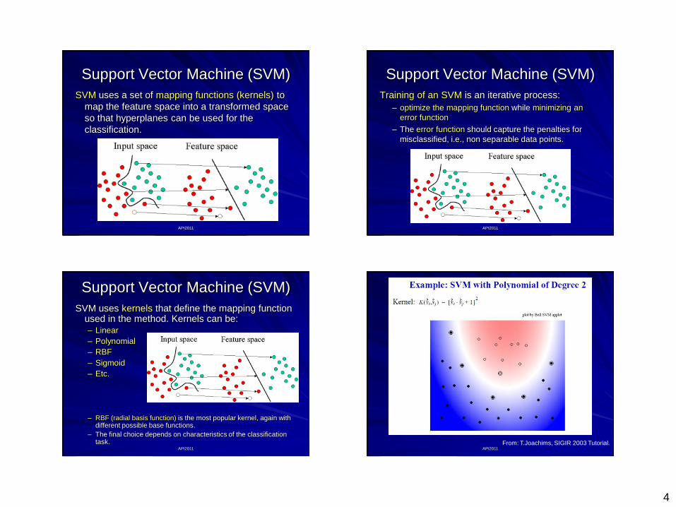
Support Vector Machine (SVM)
SVM uses a set of mapping functions (kernels) to
map the feature space into a transformed space
so that hyperplanes can be used for the
classification.
API2011
Support Vector Machine (SVM)
Training of an SVM is an iterative process:
– optimize the mapping function while minimizing an
error function
– The error function should capture the penalties for
misclassified, i.e., non separable data points.
API2011
Support Vector Machine (SVM)
SVM uses kernels that define the mapping function used in the method. Kernels can be:– Linear
– Polynomial
– RBF
– Sigmoid
– Etc.
– RBF (radial basis function) is the most popular kernel, again with different possible base functions.
– The final choice depends on characteristics of the classification task.
API2011
From: T.Joachims, SIGIR 2003 Tutorial.

5
API2011
From: T.Joachims, SIGIR 2003 Tutorial.API2011
Sequences: Sound and DNA
DNA: helix-shaped molecule
whose constituents are two
parallel strands of nucleotides
DNA is usually represented by
sequences of these four
nucleotides
This assumes only one strand
is considered; the second
strand is always derivable
from the first by pairing A‘s
with T‘s and C‘s with G‘s and
vice-versa
Nucleotides (bases)
– Adenine (A)
– Cytosine (C)
– Guanine (G)
– Thymine (T)
API2011
Biological Information:
From Genes to Proteins
GeneDNA
RNA
Transcription
Translation
Protein Protein folding
genomics
molecular
biology
structural
biology
biophysics
API2011
DNA / amino acid
sequence 3D structure protein functions
DNA (gene) →→→ pre-RNA →→→ RNA →→→ Protein
RNA-polymerase Spliceosome Ribosome
CGCCAGCTGGACGGGCACACC
ATGAGGCTGCTGACCCTCCTG
GGCCTTCTG…
TDQAAFDTNIVTLTRFVMEQG
RKARGTGEMTQLLNSLCTAVK
AISTAVRKAGIAHLYGIAGST
NVTGDQVKKLDVLSNDLVINV
LKSSFATCVLVTEEDKNAIIV
EPEKRGKYVVCFDPLDGSSNI
DCLVSIGTIFGIYRKNSTDEP
SEKDALQPGRNLVAAGYALYG
SATML
From Amino Acids to Proteins
Functions

6
API2011
Motivation for Markov Models
There are many cases in which we would like to represent the statistical regularities of some class of sequences
– genes
– proteins in a given family
– Sequences of audio features
Markov models are well suited to this type of task
API2011
A Markov Chain Model
Transition probabilities
– Pr(xi=a|xi-1=g)=0.16
– Pr(xi=c|xi-1=g)=0.34
– Pr(xi=g|xi-1=g)=0.38
– Pr(xi=t|xi-1=g)=0.12
1)|Pr( 1 gxx ii
API2011
Definition of Markov Chain Model
A Markov chain[1] model is defined by
– a set of states
some states emit symbols
other states (e.g., the begin state) are silent
– a set of transitions with associated probabilities
the transitions emanating from a given state define a distribution
over the possible next states
[1] Марков А. А., Распространение закона больших чисел на величины, зависящие друг
от друга. — Известия физико-математического общества при Казанском
университете. — 2-я серия. — Том 15. (1906) — С. 135—156
API2011
Markov Chain Models: Properties
Given some sequence x of length L
How probable the sequence is given our model?
For any probabilistic model of sequences, we can write this
probability as
Key property of a (1st order) Markov chain:
The probability of each xi depends only on the value of xi-1
)Pr()...,...,|Pr(),...,|Pr(
),...,,Pr()Pr(
112111
11
xxxxxxx
xxxx
LLLL
LL
L
i
ii
LLLL
xxx
xxxxxxxx
2
11
112211
)|Pr()Pr(
)Pr()|Pr()...|Pr()|Pr()Pr(

7
API2011
The Probability of a Sequence for a
Markov Chain Model
Pr(cggt)=Pr(c)Pr(g|c)Pr(g|g)Pr(t|g)
API2011
Example Applications
Isolated Word Recognition
A spectral vector is modeled by a state in a Markov chain
An utterance is represented by a sequence of states
Algorithmic Music Composition
States are note or pitch values
Probabilities for transitions to other notes are given (can be 1st order
or second order etc.)
API2011
Markov Chains for Discrimination
Suppose we want to distinguish CpG islands from other
sequence regions
Given sequences from CpG islands, and sequences
from other regions, we can construct
– a model to represent CpG islands
– a null model to represent the other regions
Using the models we can now score a test sequence by:
)|Pr(
)|Pr(log)(
nullModelx
CpGModelxxscore
API2011
Markov Chains for Discrimination
Why can we use
According to Bayes’ rule:
If we are not taking into account prior probabilities (Pr(CpG) and
Pr(null)) of the two classes, then from Bayes’ rule it is clear that
we just need to compare Pr(x|CpG) and Pr(x|null) as is done in
our scoring function score().
)Pr(
)Pr()|Pr()|Pr(
x
CpGCpGxxCpG
)Pr(
)Pr()|Pr()|Pr(
x
nullnullxxnull
)|Pr(
)|Pr(log)(
nullModelx
CpGModelxxscore
As the real score should be:
Assume x is observed what is the
probability that x was modeled by
CpG compared to the probability
that x was modeled by the null
model, i.e., Pr(CpG | x) / Pr(null | x)

8
API2011
Higher Order Markov Chains
The Markov property specifies that the probability of a state
depends only on the probability of the previous state
But we can build more ―memory‖ into our states by using a higher
order Markov model
In an n-th order Markov model
The probability of the current state depends on the previous n states.
),...,|Pr(),...,,|Pr( 1121 niiiiii xxxxxxx
API2011
Selecting the Order of a Markov Chain
Model
But the number of parameters we need to estimate
grows exponentially with the order
– for modeling DNA we need parameters for an n-th
order model
The higher the order, the less reliable we can expect
our parameter estimates to be
– estimating the parameters of a 2nd order Markov chain from the
complete genome of E. Coli (5.44 x 10⁶ bases) , we‘d see
each word ~ 85.000 times on average (divide by 43)
– estimating the parameters of a 9th order chain, we‘d see each
word ~ 5 times on average (divide by 410 ~ 106)
)4( 1nO
API2011
Higher Order Markov Chains
An n-th order Markov chain over some alphabet A is equivalent to
a first order Markov chain over the alphabet of n-tuples: An
Example: A 2nd order Markov model for DNA can be treated as a
1st order Markov model over alphabet
AA, AC, AG, AT
CA, CC, CG, CT
GA, GC, GG, GT
TA, TC, TG, TT
API2011
A Fifth Order Markov Chain
Pr(gctaca) = Pr(gctac) . Pr(a | gctac)

9
API2011
Hidden Markov Model: A Simple HMM
Given observed sequence AGGCT, which state emits every item?
Model 1 Model 2
API2011
Tutorial on HMM
L.R. Rabiner, A Tutorial on Hidden Markov Models
and Selected Applications in Speech
Recognition, Proceeding of the IEEE, Vol. 77,
No. 22, February 1989.
API2011
HMM for Hidden Coin Tossing
HT
T
T T
T
H
T
……… H H T T H T H H T T H
API2011
Hidden State
We‘ll distinguish between the observed parts of a
problem and the hidden parts
In the Markov models we‘ve considered previously, it is
clear which state accounts for each part of the observed
sequence
In the model above, there are multiple states that could
account for each part of the observed sequence
– this is the hidden part of the problem

10
API2011
Learning and Prediction Tasks(in general, i.e., applies on both MM as HMM)
Learning– Given: a model, a set of training sequences
– Do: find model parameters that explain the training sequences with
relatively high probability (goal is to find a model that generalizes well to
sequences we haven‘t seen before)
Classification– Given: a set of models representing different sequence classes, and
given a test sequence
– Do: determine which model/class best explains the sequence
Segmentation– Given: a model representing different sequence classes, and given a
test sequence
– Do: segment the sequence into subsequences, predicting the class of
each subsequence
API2011
Algorithms for Learning & Prediction
Learning– correct path known for each training sequence -> simple maximum
likelihood or Bayesian estimation
– correct path not known -> Forward-Backward algorithm + ML or Bayesian
estimation
Classification– simple Markov model -> calculate probability of sequence along single
path for each model
– hidden Markov model -> Forward algorithm to calculate probability of
sequence along all paths for each model
Segmentation
– hidden Markov model -> Viterbi algorithm to find most probable path for
sequence
API2011
The Parameters of an HMM
Transition Probabilities
– Probability of transition from state k to state l
Emission Probabilities
– Probability of emitting character b in state k
Note: HMM’s can also be formulated using an emission probability
associated with a transition from state k to state l.
)|Pr( 1 kla iikl
)|Pr()( kbxbe iik
API2011
An HMM Example
Emission probabilities∑ pi = 1
Transition probabilities∑ pi = 1

11
API2011
HMM Isolated Word Recognizer
API2011
Three Important Questions(See also L.R. Rabiner (1989))
How likely is a given sequence?
– The Forward algorithm
What is the most probable ―path‖ for generating
a given sequence?
– The Viterbi algorithm
How can we learn the HMM parameters given a
set of sequences?
– The Forward-Backward (Baum-Welch) algorithm
API2011
How Likely is a Given Sequence?
The probability that a given path is taken and
the sequence is generated:L
i
iNL iiiaxeaxx
1
001 11)()...,...Pr(
6.3.8.4.2.4.5.
)(
)()(
),Pr(
35313
111101
aCea
AeaAea
AAC
API2011
How Likely is a Given Sequence?
But we need the probability over all paths:
The number of paths can be exponential in the
length of the sequence...
The Forward algorithm enables us to compute
this efficiently

12
API2011
The Forward Algorithm
Define to be the probability of being in
state k having observed the first i characters of
sequence x of length L
To compute , the probability of being in
the end state having observed all of sequence
x
Can be defined recursively
Compute using dynamic programming
)(if k
)(LfN
API2011
The Forward Algorithm
fk(i) equal to the probability of being in state k having
observed the first i characters of sequence x
Initialization
– f0(0) = 1 for start state; fi(0) = 0 for other state
Recursion
– For emitting state (i = 1, … L)
– For silent state
Termination
k
klkl aifif )()(
k
klkll aifieif )1()()(
k
kNkNL aLfLfxxx )()()...Pr()Pr( 1
API2011
Forward Algorithm Example
Given the sequence x=TAGA
API2011
Forward Algorithm Example
Initialization
– f0(0)=1, f1(0)=0…f5(0)=0
Computing other values
– f1(1)=e1(T)*(f0(0)a01+f1(0)a11)
=0.3*(1*0.5+0*0.2)=0.15
– f2(1)=0.4*(1*0.5+0*0.8)
– f1(2)=e1(A)*(f0(1)a01+f1(1)a11)
=0.4*(0*0.5+0.15*0.2)
…
– Pr(TAGA)= f5(4)=f3(4)a35+f4(4)a45

13
API2011
Three Important Questions
How likely is a given sequence?
What is the most probable ―path‖ for generating
a given sequence?
How can we learn the HMM parameters given a
set of sequences?
API2011
Finding the Most Probable Path: The Viterbi Algorithm
Define vk(i) to be the probability of the most probable
path accounting for the first i characters of x and
ending in state k
We want to compute vN(L), the probability of the most
probable path accounting for all of the sequence and
ending in the end state
Can be defined recursively
Again we can use use Dynamic Programming to
compute vN(L) and find the most probable path
efficiently
API2011
Finding the Most Probable Path: The Viterbi Algorithm
Define vk(i) to be the probability of the most probable
path π accounting for the first i characters of x and
ending in state k
The Viterbi Algorithm:
1. Initialization (i = 0)
v0(0) = 1, vk(0) = 0 for k>0
2. Recursion (i = 1,…,L)
vl(i) = el(xi) .maxk(vk(i-1).akl)
ptri(l) = argmaxk(vk(i-1).akl)
3. Termination:
P(x,π*) = maxk(vk(L).ak0)
π*L = argmaxk(vk(L).ak0)
API2011
Three Important Questions
How likely is a given sequence?
What is the most probable ―path‖ for
generating a given sequence?
How can we learn the HMM parameters
given a set of sequences?
14
API2011
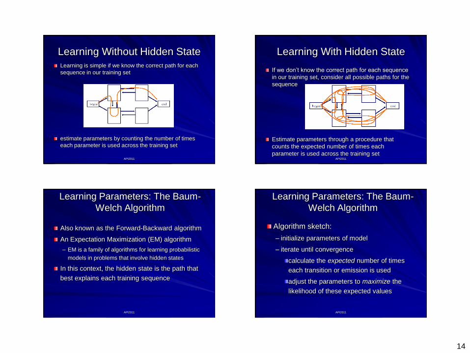
Learning Without Hidden State
Learning is simple if we know the correct path for each
sequence in our training set
estimate parameters by counting the number of times
each parameter is used across the training set
API2011
Learning With Hidden State
If we don‘t know the correct path for each sequence
in our training set, consider all possible paths for the
sequence
Estimate parameters through a procedure that
counts the expected number of times each
parameter is used across the training set
API2011
Learning Parameters: The Baum-
Welch Algorithm
Also known as the Forward-Backward algorithm
An Expectation Maximization (EM) algorithm
– EM is a family of algorithms for learning probabilistic
models in problems that involve hidden states
In this context, the hidden state is the path that
best explains each training sequence
API2011
Learning Parameters: The Baum-
Welch Algorithm
Algorithm sketch:
– initialize parameters of model
– iterate until convergence
calculate the expected number of times
each transition or emission is used
adjust the parameters to maximize the
likelihood of these expected values
15
API2011
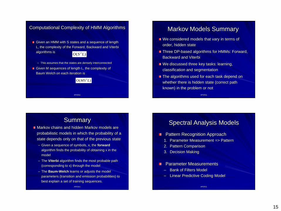
Computational Complexity of HMM Algorithms
Given an HMM with S states and a sequence of length
L, the complexity of the Forward, Backward and Viterbi
algorithms is
– This assumes that the states are densely interconnected
Given M sequences of length L, the complexity of
Baum Welch on each iteration is
)( 2LSO
)( 2LMSO
API2011
Markov Models Summary
We considered models that vary in terms of
order, hidden state
Three DP-based algorithms for HMMs: Forward,
Backward and Viterbi
We discussed three key tasks: learning,
classification and segmentation
The algorithms used for each task depend on
whether there is hidden state (correct path
known) in the problem or not
API2011
SummaryMarkov chains and hidden Markov models are
probabilistic models in which the probability of a
state depends only on that of the previous state
– Given a sequence of symbols, x, the forward
algorithm finds the probability of obtaining x in the
model
– The Viterbi algorithm finds the most probable path
(corresponding to x) through the model
– The Baum-Welch learns or adjusts the model
parameters (transition and emission probabilities) to
best explain a set of training sequences.
API2011
Spectral Analysis Models
Pattern Recognition Approach
1. Parameter Measurement => Pattern
2. Pattern Comparison
3. Decision Making
Parameter Measurements
– Bank of Filters Model
– Linear Predictive Coding Model

16
API2011
Band Pass Filter
Audio Signal
s(n)
Bandpass Filter
F()
Result Audio Signal
F(s(n))
Note that the bandpass filter can be
defined as:
• a convolution with a filter response
function in the time domain,
• a multiplication with a filter response
function in the frequency domain
API2011
Bank of Filters Analysis Model
API2011
Bank of Filters Analysis Model
Speech Signal: s(n), n=0,1,…– Digital with Fs the sampling frequency of s(n)
Bank of q Band Pass Filters: BPF1, …,BPFq
– Spanning a frequency range of, e.g., 100-3000Hz or 100-16kHz
– BPFi(s(n)) = xn(ejωi), where ωi = 2πfi/Fs is equal to the
normalized frequency fi, where i=1, …, q.
– xn(ejωi) is the short time spectral representation of s(n)
at time n, as seen through the BPFi with centre frequency ωi, where i=1, …, q.
Note: Each BPF independently processes s to produce the spectral representation x
API2011
MFCCs
Mel-Scale
Filter Bank
MFCC‘s
first 12 most
Significant
coefficients
Log()
Speech
Audio, …Preemphasis Windowing
Fast Fourier
Transform
Direct Cosine
Transform
MFCCs are calculated using the formula:
N
k
iki NkXC1
)/)5.0(cos(
Where
• Ci is the cepstral coefficient (i from {1, …, 12}
• P the order (12 in our case)
• K the number of discrete Fourier
transform magnitude coefficients
• Xk the kth order log-energy output
from the Mel-Scale filterbank.
• N is the number of filters

17
API2011
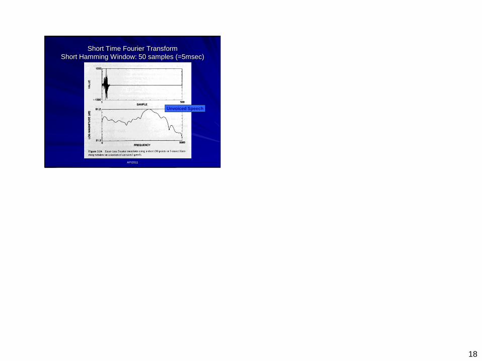
Short Time Fourier Transform
• s(m) signal
• w(n-m) a fixed low pass window
API2011
Short Time Fourier Transform
Long Hamming Window: 500 samples (=50msec)
Voiced Speech
API2011
Short Time Fourier Transform
Short Hamming Window: 50 samples (=5msec)
Voiced Speech
API2011
Short Time Fourier Transform
Long Hamming Window: 500 samples (=50msec)
Unvoiced Speech
18
API2011
Short Time Fourier Transform
Short Hamming Window: 50 samples (=5msec)
Unvoiced Speech