Attribute Discretization and Selection...
38
Attribute Discretization and Selection Clustering NIKOLA MILIKI Ć [email protected] URO Š KR Č ADINAC [email protected]
Transcript of Attribute Discretization and Selection...

Attribute Discretization and Selection Clustering
NIKOLA MILIKIĆ [email protected]
UROŠ KRČADINAC [email protected]

Naive Bayes Features
• Intended primarily for the work with nominal attributes
• In case of numeric attributes
• Use the propability distribution of attributes (Normal distribution is default) for probability estimation for the each attribute
• Discretize the attribute’s values

Attribute Discretization
Discretization is the process of tranformation numeric data into nominal data, by putting the numeric values into distinct groups, which lenght is fixed.
Common approaches:
• Unsupervised:
• Equal-width binning
• Equal-frequency binning
• Supervised – classes are taken into account

Equal-Width Binning
Equal-width binning divides the scope of possible values into N subscopes (bins) of the same width:
Example: If the scope of the values is between 0 and 100, we should create 5 subscopes (bins) in the following manner:
Width = (100 – 0) / 5 = 20
Subscopes (bins): [0-20], (20-40], (40-60], (60-80], (80-100]
Usually, the first and the final subscope (bin) are being expended in order to include possible values outside the original scope.
width = (max value – min value) / N

Equal-frequency binning
Equal-frequency binning (or equal-height binning) divides the scope of possible values into N subscopes where each subscope (bin) carries the same number of instances:
Example: We want to put the following values in 5 subscopes (bins):
5, 7, 12, 35, 65, 82, 84, 88, 90, 95
So, each subscope will have 2 instances:
5, 7,|12, 35,| 65, 82,| 84, 88,| 90, 95

Discretization in Weka
We apply certain Filters to attributes we want to discretize.
Preprocess tab Option: Choose -> Filter filters/unsupervised/attribute Discretize.
FishersIrisDataset.arff

Discretization in Weka
Equal-width binning is the default option.
• attributeIndices – the first-last value means that we are discretizing all values. We can also name the attribute numbers.
• bins – the desired number of
scopes (bins) • useEqualFrequency – false by
default; true if we use Equal Frequency binning

Discretization in Weka Applying the filter
The resulting subscopes (bins)

Data, before and after discretization Before
After

Attribute Selection
Attribute Selection (or Feature Selection) is the process of choosing a subset of relevant attributes that will be used during the further analysis.
It is being applied in cases where the dataset contains attributes which are redudant and/or irrelevant.
• Redundant attributes are the ones that do not provide more information than the attributes we already have in our dataset.
• Irrelevant attributes are the ones that are useless in the context of the current analysis.

Attribute Selection Advantages
Excessive attributes can degrade the performance of the model.
Advantages:
• Advances the readability of the model (because now the model contains only the relevant attributes)
• Shortens the training time
• Generalization power is higher because it lowers the possibility of overfitting
If the problem is well-known, the best way to select attribute is to do it manually. However, automated apporaches also give good results.

Approaches to Attribute Selection
Two approaches:
• Filter method – use the approximation based on the general features of the data.
• Wrapper method – attribute subsets are being evaluated by using the maching learning algorithm, applied to the dataset. The name Wrapper comes from the fact that the algorithm is wrapped within the process of selection. The chosen subset of attributes is the one for which the algorithm gives the best results.

Attribute Selection Example census90-income.arff

Attribute Selection Example
We want to apply the
selection of attributes

Attribute Selection Example
ClassifierSubsetEval is our choice for the
evaluator

Attribute Selection Example
NaiveBayes classifier
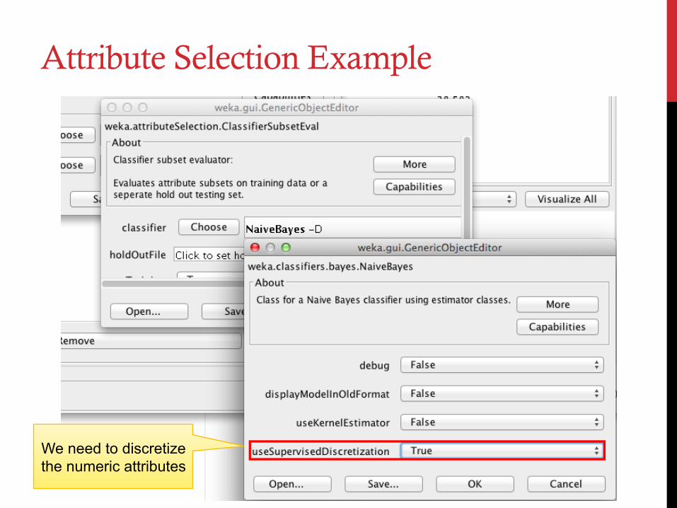
Attribute Selection Example
We need to discretize the numeric attributes

Attribute Selection Example
As the search method we choose the BestFirst

Attribute Selection Example
Filter is set and can be applied

Attribute Selection Example
The number of attributes is reduced to 7

Clustering
Clustering belongs to a group of techiques of unsupervised learning. It enables grouping instances into groups, where we know which are the possible groups in advance.
These groups are called clusters.
As the result of clustering each instance is being added a new attribute – the cluster to which it belongs. The clustering is said to be successful if the final clusters make sense, if they could be given meaningful names.

K-Means algorithm in Weka FishersIrisDataset.arff

Choosing the clustering algorithm
Cluster tab
We choose the SimpleKMeans
algorithm
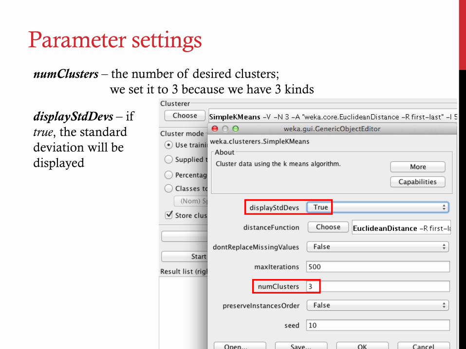
Parameter settings numClusters – the number of desired clusters;
we set it to 3 because we have 3 kinds
displayStdDevs – if true, the standard deviation will be displayed

Running the Clustering
Clustering over the imported data
We ignore the Species
attribute

Results of Clustering
Centroids of each cluster and their
standard deviations
Number of instnaces in each cluster

Evaluation of Results
Select the attrubute which we want to
compare the results with.
Which classes are in which clusters
Names of classes which are given to
clusters

Visualization of Clusters
Right click
Visual representation
of clusters

Was clustering successful?
Within cluster sum of squared error gives us the assessment of quality
Vrednosti centroida po
svim atributima
It is being counted as the sum of square differences between the value of the attribute of each instance
and the value of the centroid of the given
attribute
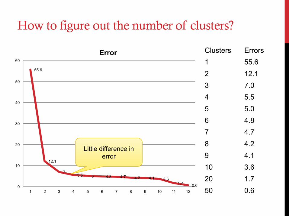
How to figure out the number of clusters?
55.6
12.1
7 5.5 5 4.8 4.7 4.2 4.1 3.6
1.7 0.6 0
10
20
30
40
50
60
1 2 3 4 5 6 7 8 9 10 11 12
Error Clusters Errors 1 55.6 2 12.1 3 7.0 4 5.5 5 5.0 6 4.8 7 4.7 8 4.2 9 4.1 10 3.6 20 1.7 50 0.6
Little difference in error

Using Clusters for Classification
AddCluster – our choice of the filter
Setting no class

Using Clusters for Classification
We choose the SimpleKMeans as the
clustering algorithm
In terms of clustering, we ignore the attribute
5 (Speices)

Using Clusters for Classification
After the filter is being applied (Apply) we add the new attribute by the name
of cluster

Using Clusters for Classification
Optional: this attribute can be removed before we create a clasification
model

Using Clusters for Classification
We use the NaiveBayes
classifier
We do the classification according to the cluster
attribute
The confusion matrix

Weka Tutorials and Assignments @ The Technology Forge
• Link: http://www.technologyforge.net/WekaTutorials/
Thank you notes
Witten, Ian H., Eibe Frank, and Mark A. Hall. Data Mining: Practical Machine Learning Tools and Techniques: Practical Machine Learning Tools and Techniques. Elsevier, 2011.

A survey for you, to judge us :) http://goo.gl/cqdp3I