Computation of a face attractiveness index based on neoclassical canons,

symmetry, and golden ratios

Kendra Schmid1, David Marx1 and Ashok Samal2

1Department of Statistics, 2Department of Computer Science and Engineering

University of Nebraska-Lincoln

Lincoln, NE 68588-0115

Abstract

Analysis of attractiveness of faces has long been a topic of research. Literature has

identified many different factors that can be related to attractiveness including symmetry,

averageness, sexual dimorphism and adherence to the Golden Ratio. In this research we

systematically analyze the role of three factors: symmetry, conformance to Neoclassical

Canons and the Golden Ratio in the determination of attractiveness of a face. Unlike

many researchers, we focus on the geometry of a face and use actual faces in

standardized databases for our analysis. Our results are in agreement with the literature in

that males and females generally agree on which faces are viewed as attractive and which

are not. However, there are some differences in the criteria used by males and females to

determine attractiveness. Using statistical analyses, we have developed a model to predict

the attractiveness of a face using its geometry. The results show that our model is

accurate with low residual errors.

Key Words: Face Attractiveness, Face Recognition, Neoclassical Canons, Face

Symmetry, Golden Ratio

1. Introduction

A popular axiom concerning physical attractiveness is: “Beauty is in the eye of the

beholder”. Research in the area of facial perception has identified many different factors

that contribute to a face being considered attractive. Armstrong (2004) suggests that

beauty cannot be defined by one single principle. Rhodes (2006) focuses on averageness,

1

symmetry, and sexual dimorphism and their link to facial attractiveness. Little et al.

(2000) suggests that self-perceived attractiveness influences one’s opinion of the

attractiveness of others, and DeBruine (2004) shows both males and females prefer faces

that resemble their own.

In this paper, we develop a quantitative method for measuring facial attractiveness using

a combination of several factors that have been deemed significant in previous research.

Many previous studies have used composite faces (combinations of several faces) or

faces that are altered in some other way to study the effects of symmetry and averageness

on attractiveness (Kowner 1996, Langolis 1990, Langolis et al. 1994, Little & Hancock

2002, O’Toole et al. 1999, Perrett et al. 1998, Perrett et al. 1999, Rhodes 2006, Rhodes et

al. 1998, Rhodes et al. 1999, Rhodes & Tremewan 1996, Swaddle & Cuthill 1995). In

contrast, we use the actual faces compiled from a standard face recognition database for

our analysis. We then determine the location of important landmarks in the face (Farkas

1994, Farkas & Munro 1987). In all, we use 29 landmarks on each face as described by

Shi et al. (2006) to take physical measurements. Using these landmarks, we compute the

values of three factors: Neoclassical Canons, symmetry, and golden ratios. These faces

are presented to a set of human subjects to determine their perceived attractiveness using

a partially balanced incomplete block design to find which of these or which combination

of these is the best predictor of attractiveness. Using a statistical approach, we

systematically investigate the relationship between the facial measurements in the images

and the attractiveness ratings given by the human participants.

2

In addition to which measure (canons, symmetry, or golden ratios) best predicts

attractiveness, we are able to identify which features play the greatest role in

attractiveness and if these features are common across both genders of raters and images.

Rhodes (2006) suggests that it may be wise to distinguish same sex ratings from opposite

sex ratings. We record the gender of the rater and the image to explore the differences or

similarities in how males and females view attractiveness in images of the same and

opposite gender.

We describe the image database used for our research in Section 2. We also explain how

the measurements are obtained and the design of our human studies experiment. In

Section 3 we discuss the methods to compute the attractiveness predictors from face

images. The predictors are based on Neoclassical Canons, symmetry, and golden ratios,

which are described in literature. However, we provide new approaches to compute these

predictors. In Section 4, we present the details of our statistical analyses and the

associated results. The features in the face that are the best predictor of attractiveness are

described in this section. Finally, we summarize our findings and identify areas for

future work in Section 5.

2. Datasets and Experimental Design

We begin with an image database containing a set of face images for our experiment and

analysis. Using the image database, we compile two datasets for our analysis. The

feature dataset consists of the locations of the landmarks in the faces. The attractiveness

dataset contains the attractiveness ratings given to the images by the human participants.

3

We briefly describe the image database and the process of creating the features and

attractiveness datasets in this section.

2.1. The Image Database

The majority of the images used in this research were taken from the Facial Recognition

Technology (FERET) Database (Phillips et al. 2000). The FERET Database contains

some fourteen thousand facial images that were collected by photographing over one

thousand subjects at various poses. The images were collected over the course of fifteen

sessions between 1993 and 1996. Some individuals were photographed multiple times,

sometimes with more than two years separating their first and last sitting.

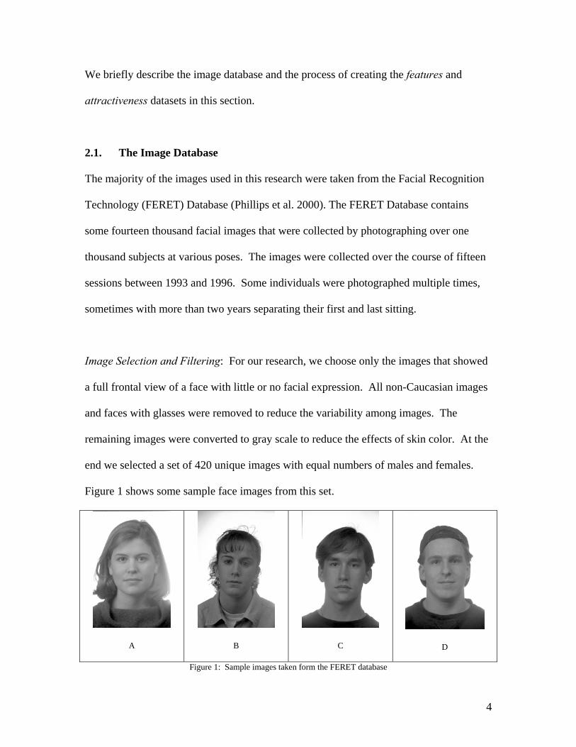
Image Selection and Filtering: For our research, we choose only the images that showed

a full frontal view of a face with little or no facial expression. All non-Caucasian images

and faces with glasses were removed to reduce the variability among images. The

remaining images were converted to gray scale to reduce the effects of skin color. At the

end we selected a set of 420 unique images with equal numbers of males and females.

Figure 1 shows some sample face images from this set.

A

B

C

D

Figure 1: Sample images taken form the FERET database

4

In addition to the images from the FERET Database, we used the images of 32 popular

movie personalities ranging from the 1930’s until the present day (Movie Actor Index).

Again, an equal number of male and female faces were used. The personalities were

chosen to include only those that were considered to be attractive. Our motivation for

including such faces, deemed more attractive than the norm by the society, was to verify

our system of rating faces; the ratings given to these faces would be expected to be

significantly higher than the ratings given to the faces of non-famous people. Figure 2

shows some sample face images from this set.

Greta Garbo

Meg Ryan

Rock Hudson

Keanu Reeves

Figure 2: Sample images of faces known to be attractive.

2.2. The Feature Point Database

We developed a tool to derive measurements from a set of standard face images using a

graphical user interface. A set of 29 important landmarks was identified based on existing

literature (Farkas 1994). A reference image showing the location of the features and the

test image is presented. The user is prompted to locate the corresponding feature in the

test image. The user indicates the location of the feature by a mouse click. Table 1

provides the description of each of these feature points. Using this tool we extracted all

5

29 feature points from each of the 452 face images. Figure 3 shows the layout of the

landmarks on a face image. The feature point database consists of the locations of the

feature points for the faces from the FERET database and the faces of famous people.

Feature Point Feature Description

01 The point on the hairline in the midline of the forehead 02 Highest point on upper borderline in mid portion of left eyebrow 03 Most prominent midline point between eyebrows 04 Highest point on upper borderline in mid portion of right eyebrow 05 Highest point on the free margin of left ear 06 Most prominent lateral point on left side of the skull 07 Highest point on lower border of left eyebrow 08 Highest point on lower border of right eyebrow 09 Most prominent lateral point on right side of the skull 10 Highest point on the free margin of right ear 11 Point at outer right side of the eye. 12 Point at inner right side of the eye 13 Point at inner left side of the eye 14 Point at outer left side of the eye. 15 Lowest point on lower margin left eye 16 Lowest point on lower margin right eye 17 Lowest point of left ear 18 Most lateral point on left side of nose 19 Midpoint of nose 20 Most lateral point on right side of nose 21 Lowest point of right ear 22 Highest point on left side of lip 23 Midpoint on upper lip 24 Highest point on right side of lip 25 Left most point of closed lip 26 Midpoint of closed lip 27 Right most point of closed lip 28 Point on lower border of lower lip or upper border of chin 29 Tip of chin

Table 1: Description of feature points

6

Figure 3: Feature points on an image

2.3. Attractiveness Scores Database

In order to get some ground truth on the attractiveness of faces in our database, we

compiled their attractiveness scores using human subjects. The human subjects were

asked to rate the faces in the database using a ten-point scale. We use these scores to

build a database of the attractiveness for the faces.

Design of Experiment: Asking a subject to rate all 452 faces would not only take a long

time, but would reduce the quality of the results. Therefore, we chose a partially

balanced incomplete block design for this process. The 420 FERET images were split

into six groups of 70 images, labeled A, B, C, D, E, and F with each group consisting of

35 males and 35 females. In addition, each group has a total of 30 duplicate images with

fifteen male duplicates and fifteen female duplicates, for a total of 100 images per group.

Each participant was assigned to rate two of these groups. Including the duplicates

7

provides a way to check the consistency within each rater. In addition to these 200

images, each subject was asked to rate each of the famous faces. Thus, each subject gave

ratings to 232 faces in all.

We chose a partially balanced design instead of a balanced design because the latter

would require fifteen raters which would not allow for an equal number of male and

female raters. In our design, each rater is assigned two of the six groups of images so that

no two groups appear together more than once and so each group is shown to two male

and two female raters. Table 2 shows the layout of the design.

Participant ID Gender Groups Shown

1 M A, C 2 M B, F 3 M D, E 4 M A, D 5 M B, C 6 M E, F 7 F A, E 8 F B, D 9 F C, F 10 F A, F 11 F B, E 12 F C, D

Table 2: Partially Balanced Incomplete Block Design

Participant Selection and Data Collection: Twelve participants (raters) were chosen from

students and employees at the University of Nebraska-Lincoln and ranged in age from 19

to 61 years. An equal number of male and female participants (six of each) were chosen

to rate the faces. Using twelve participants allowed for the partially balanced incomplete

block design while maintaining an equal number of male and female raters. The gender

and age of each participant were collected and stored in the database.

8

Each of the six groups of images was shown to four raters, two males and two females.

Each rater viewed two of the six groups of images in a random sequence and the

experiment was designed so that no raters viewed the same two groups. After viewing

the 200 images, each rater viewed the 32 famous images. Each participant rated each

face image on a scale from 1 (least attractive) to 10 (most attractive) based on his or her

opinion. In addition to the score given by the rater, we record the time taken to give the

ratings. After rating the 232 images, the participant is given the option to rate him or

herself using the same 10 point attractiveness scale.

The experimental design was repeated three times, using different raters in each instance,

for a total of 36 raters. Within each group of twelve raters, each image was shown four

times, each duplicated image was shown eight times, and each famous image was shown

twelve times.

Data Filtering: After the attractiveness scores were collected, we examined the integrity

of the data. We calculated the variance of the ratings given by each user. A variance of

zero indicates that a participant gave the same rating to each face and hence the scores of

this rater should be ignored. We also examined the raters whose scores had very large or

very small variances. A very small variance could indicate a participant going back and

forth between two consecutive numbers. A very large variance could indicate a pattern

where a participant goes back and forth between two numbers such as 1 and 10, or just

goes up and down from 1 to 10. We also examined the time spent to rate the faces by

each participant. A very small amount of time to complete the rating process could

9

indicate a participant just clicking numbers and not actually rating while a very large

amount of time might mean that the participant was interrupted during the rating process.

If a rater was flagged for any of the above problems, the corresponding ratings (and the

time taken to rate) were examined more carefully. The scores that did not have a high

level of integrity were removed.

3. Computation of Attractiveness Predictors

The main motivation of our research is to examine the attractiveness of a face, Fi, as a

function of its face geometry. The geometry of a face is captured by a set of m landmarks.

Thus:

Fi = {fi1, fi2, …, fim},

where each feature point is represented by its two dimensional spatial coordinates in the

face. Thus,

fij = (xij, yij), 1≤ i ≤ n, 1≤ j ≤ m.

Our goal is to determine a function A that maps a face to an attractiveness score.

A(Fi) → [1,10]

To compute the attractiveness, we use three predictors that have been proposed in

literature: Neoclassical Canons, Face Symmetry, and Golden Ratios. We discuss each of

them below.

3.1. Neoclassical Canons

Neoclassical Canons view the face in proportions and have been proposed by artists

dating back to the renaissance period as guides to drawing beautiful faces (Farkas et al.

10

1985). The basic premise is that portions of an attractive face should follow certain

defined ratios. Farkas et al. (1985) summarizes these principles in nine Neoclassical

Canons and their variations. Four of the canons deal with vertical measurements, four

with horizontal measurements, and one with angles of inclination. Only six of these can

be tested from the frontal views of the images. Therefore, only those six canons (listed in

Table 3) are used to investigate their relationship with attractiveness of a face.

Formula No. Description 2 Forehead height = Nose length = Lower face height 4 Nose length = Ear length 5 Interocular distance = Nose width 6 Interocular distance = Right or left eye fissure width 7 Mouth width = 1.5 × Nose width 8 Face width = 4 × Nose width

Table 3: Description of Neoclassical Canons (Formula number given by Farkas (1985))

As shown in Table 3, some canons use two measurements (e.g. Formula 4 and 8) while

others use three (e.g. Formula 2, 6). To consistently measure compliance with the canons

(i.e. equality to proposed ratios) with different numbers of features, we use the coefficient

of variation. The coefficient of variation is defined as the ratio of the standard deviation

of the distances to the mean of the distances. For a canon with three distances, using a

ratio would require pair-wise comparisons of these distances, but using the coefficient of

variation allows us to incorporate all three distances into one value while adjusting for the

size of the face (dividing by the mean). A value of zero for the coefficient of variation

says there is no variation in the distances (they are equal). For non-zero values, the larger

the value, the more the face differs from the canon. Using this approach, we compute the

degree of match with each canon (i.e. coefficient of variation) for all the faces and store it

in a database.

11

3.2. Symmetry

Symmetry for a face is considered to be an important factor for attractiveness (Rhodes

2006). Symmetry has been defined in many different ways (Grammer & Thornhill 1994,

Kowner 1996, Little & Jones 2006, Penton-Voak et al. 2001, Perrett et al. 1999, Rhodes

et al. 1998, Rhodes et al. 1999, Rhodes 2006, Samuels et al. 1994, Scheib et al. 1999,

Swaddle & Cuthill 1995); however, many consider only the symmetry about a vertical

axis. We define the axis of symmetry to be located vertically at the middle of the face.

We determine this line by fitting the least squares regression line through the seven points

measured along the middle of the face (Points 1, 3, 19, 23, 26, 28, 29 shown in Figure 3).

We use the following feature pairs (left and right) for our analysis of symmetry.

• Eyebrows (Points 2 and 4; Points 7 and 8)

• Eyes (Points 11 and 14; Points 12 and 13; Points 15 and 16)

• Nose (Points 18 and 20)

• Ears (Points 5 and 10; 17 and 21)

• Lips (Points 22 and 24; 25 and 27),

• Face (Points 6 and 9)

In order to compute the symmetry of a face about the vertical axis, and assuming that

there are p symmetric pairs of feature points, a face, Fi, can be represented as:

Fi = {sfi1, sfi2, …, sfip},

where sfij is a symmetric pair of feature points (left (L) and right (R)) represented by:

sfij = < fijL , fijR>, fijL∈ Fi, fijR∈ Fi, 1≤ I ≤ n, 1≤ j ≤ p

and each feature point is given by its two dimensional coordinates on the face:

12

fijL = (xijL, yijL) and fijR = (xijR , yijR).

If we assume that the line of symmetry is vertical, a feature pair is perfectly symmetric if

yijL = yijR and xs- xijL = xijR- xs,

where xs=0 represents the vertical line of symmetry.

Figure 4: Line of symmetry (l), a pair of symmetric feature points, and angles

To compute the symmetry of a face, we first compute the symmetry of the individual

features. Symmetry can be computed using many different rules. Literature in sexual size

dimorphism (SSD) (Smith 1999), for example, has identified many formulas to compare

the measurements for males and females. SSD uses differences or ratios of features to

help in determining the degree of difference between male and female measurements. In

our case, we use some of the same indices to determine the degree of difference between

α

α( , )ijL ijLy

( , )ijR ijRx y

( , )ijR ijLx x y

l

ijLd ijRd

( , )ijC ijCx y

ijRh

ijLh

13

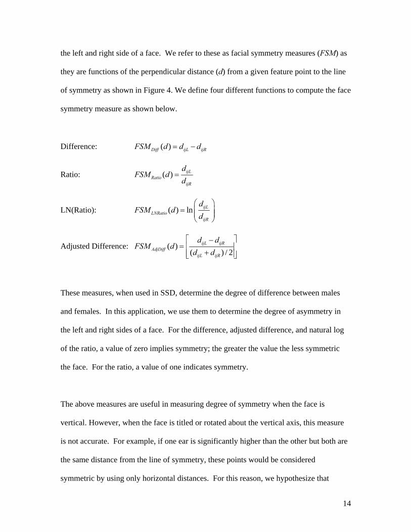
the left and right side of a face. We refer to these as facial symmetry measures (FSM) as

they are functions of the perpendicular distance (d) from a given feature point to the line

of symmetry as shown in Figure 4. We define four different functions to compute the face

symmetry measure as shown below.

Difference: ( )Diff ijL ijRFSM d d d= −

Ratio: ( ) ijLRatio

ijR

dFSM d

d=

LN(Ratio): ( ) ln ijLLNRatio

ijR

dFSM d

d⎛ ⎞

= ⎜ ⎟⎜ ⎟⎝ ⎠

Adjusted Difference: ( )( ) /

ijL ijRAdjDiff

ijL ijR

d dFSM d

d d 2⎡ ⎤−

= ⎢ ⎥+⎢ ⎥⎣ ⎦

These measures, when used in SSD, determine the degree of difference between males

and females. In this application, we use them to determine the degree of asymmetry in

the left and right sides of a face. For the difference, adjusted difference, and natural log

of the ratio, a value of zero implies symmetry; the greater the value the less symmetric

the face. For the ratio, a value of one indicates symmetry.

The above measures are useful in measuring degree of symmetry when the face is

vertical. However, when the face is titled or rotated about the vertical axis, this measure

is not accurate. For example, if one ear is significantly higher than the other but both are

the same distance from the line of symmetry, these points would be considered

symmetric by using only horizontal distances. For this reason, we hypothesize that

14

incorporating both angle and distance into the measure of symmetry will result in better

predictions of attractiveness scores than by using distances alone. Figure 4 shows a pair

of feature points (xijL , yijL) and (xijR , yijR) with the line of symmetry, l. The points are

considered symmetric if α = 0 and dijL=dijR. The angles are calculated as follows:

1tan ijR ijL

ijL ijR

y yd d

α −⎛ ⎞−⎜ ⎟=⎜ ⎟+⎝ ⎠

.

We don’t consider a vertical distance measure, even though like angles, it is not affected

by slight tilts in the face. The vertical distance can be calculated by simply subtracting

the y-coordinates of the paired feature points and using the absolute value of that

difference as a measure of symmetry, |yijL-yijR|. The problem, however, is that it is only a

single value for each pair of feature points that will be dependent on the size of the face.

When using horizontal distance, there are two measures, dijL and dijR, for each pair of

feature points. There is no obvious line of reference for vertical distances like the line of

symmetry when using horizontal distances. Furthermore, using vertical measures, in

addition to angles and horizontal distances, does not result in increased information, since

the three measures are related. Therefore, we use only the horizontal distances and

angles to compute the symmetry of a face. Together they measure both the horizontal and

vertical symmetries in the face.

3.3. Golden Ratios

While there is no systematic published study that shows any correlation between

attractiveness and proportions in face measurements that approach the Golden Ratio, such

15

relationships have been reported in popular literature (Meisner 2006, Narain 2003).

According to these reports, faces that have features with ratios close to the Golden Ratio

are thought to be aesthetically pleasing. To determine the validity of this claim, we

systematically analyzed all the ratios in the face that can be determined from the set of 29

feature points we have identified in the face. Using all ratios derived from using the pair-

wise horizontal and vertical distances all 406 possible pair-wise combinations of the 29

feature points results in 659,344 ratios per face. Each ratio was then averaged over all of

the images and standardized (subtract the Golden Ratio and divide by the standard

deviation of that ratio over all images) to see if it is close to the Golden Ratio. A

standardized value of zero indicates that when averaged over the images, that ratio is

close to the Golden Ratio. Using only ratios with standardized values less than 0.001

away from zero resulted in a set of 70 ratios. These ratios are likely to be closest to the

Golden Ratio. However, a detailed analysis of the features showed that they do not have

good intuitive descriptions (e.g. ratio of the horizontal distance from point 2 (top of

eyebrow) to 17 (bottom of ear) with the vertical distance from point 4 (top of eyebrow) to

14 (outer corner of eye)). Therefore, they were dropped from further analysis.

We also analyze a set of ratios defined by Meisner (2006) and Narain (2003) as being

equal to the Golden Ratio and as related to attractiveness of a face. With the points

available in this study, there are seventeen ratios used to explore their relationship to

attractiveness. Table 4 describes these ratios and identifies the points used for each,

where x or y refers to the x-coordinate or y-coordinate of the points and the numbers

indicate which points from Figure 3 were used in calculating the ratio.

16

Ratio Number

Numerator Points

Denominator Points Description

1 y10-y21 x12-x13 Ear length to Interocular distance 2 y10-y21 x18-x20 Ear length to Nose width 3 x15-x16 x12-x13 Mideye distance to Interocular distance 4 x15-x16 x18-x20 Mideye distance to Nose width 5 x25-x27 x12-x13 Mouth width to Interocular distance 6 y23-y29 x12-x13 Lips - chin distance to Interocular distance 7 y23-y29 x18-x20 Lips – chin distance to Nose width 8 x12-x13 x12-x11 Interocular distance to Eye fissure width 9 x12-x13 y23-y28 Interocular distance to Lip height

10 x18-x20 x12-x11 Nose width to Eye fissure width 11 x18-x20 y23-y28 Nose width to Lip height 12 x12-x11 y19-y26 Eye fissure width to Nose – mouth distance 13 y23-y28 y19-y26 Lip height to Nose – mouth distance 14 y1-y29 x17-x21 Length of face to Width of face 15 y19-y29 y26-y29 Nose – chin distance to Lips – chin distance 16 x18-x20 y19-y26 Nose width to Nose – mouth distance 17 x25-x27 x18-x20 Mouth width to Nose width

Table 4: Golden Ratios obtained from Meisner 2006 and Narain 2003

4. Analyses and results

We begin with the examination of a set of general questions about the attractiveness of

human faces. First the variability in the raters as a function of both the gender of the rater

and the gender of the face is examined. Then we examine if the self-perceived

attractiveness has any effect on the ratings given by the rater as proposed by Little et al.

(2001). Finally the relationship between the time taken by the rater and the ratings given

to the faces is analyzed.

Later we examine in depth the roles of the three predictor variables: Neoclassical Canons,

symmetry and the Golden Ratio, used in this research. We conclude this section by

analyzing how the three predictor variables can be combined to develop a predictive

model to determine attractiveness. For all our analysis we use the SAS statistical analysis

software (SAS Institute 2003).

17

4.1 Do males and females rate faces differently?

It has been reported in literature that males and females generally agree on attractiveness

(Langlois et al. 2000). In order to examine this systematically, we carried out an analysis

of variance (ANOVA) to determine if there is a difference in ratings given by men and

ratings given by women. We also wanted to examine if the gender of the face had an

impact on the rating, and if the ratings given by males and females were consistent for

male and female faces. In this analysis, the response (dependent) variable is the average

rating (AR) of the image by each participant. The ratings of duplicate images were

averaged for each rater. The following statistical model was used for the analysis.

( ) ( ) ( * )ijkl i ij k kl ik ijklAR S P S G I G S G e= + + + + +

i = 1,2 j = 1,…,18 k = 1,2 l = 1,…,116,

where S is the effect due to gender of the participant, P(S) is the random effect due to

participant, G is the effect of image gender, I(G) is the random effect due to image, S*G

is the interaction effect due to the gender of the participant and gender of the image, and e

is residual error. Central conclusions of our analysis are summarized below:

• There is no significant interaction effect between the gender of the face and the

gender of the rater. This means that the way male and female participants rated

the faces did not differ depending on the gender of the image (p = 0.5024).

• There was a slight difference in how men and women rated faces overall (p =

0.0571), with males rating faces higher than females.

• Female faces are rated significantly higher than male faces (p = 0.0004) by both

male and female raters.

18

Table 5 summarizes the attractiveness scores given by the raters. The ratings are

separated by gender of the faces and the participants. The overall averages (a) are the

average ratings given or received overall by males and females. For example, the female

images were rated at an average of 4.8997 when the gender of the rater is not considered

and the average rating of all images by all participants was 4.7308.

Participant Female Male Overall

Female 4.3597 (n) 7.4656 (f) 4.5887 (a)

5.1044 (n) 7.4179 (f) 5.2106 (a)

4.7321 (n) 7.4418 (f) 4.8997 (a)

Male 4.0845 (n) 7.0915 (f) 4.2952 (a)

4.7025 (n) 7.1750 (f) 4.8283 (a)

4.3934 (n) 7.1333 (f) 4.5618 (a)

Image

Overall 4.2221 (n) 7.2786 (f) 4.4419 (a)

4.9034 (n) 7.2965 (f) 5.0195 (a)

4.5628 (n) 7.2876 (f) 4.7308 (a)

Table 5: Summary of attractiveness ratings (n): Non-famous (FERET) faces, (f): Famous faces, (a): All the faces

When the faces were separated into famous (f) and non-famous (n), the results were fairly

consistent. For the non-famous faces, the ratings given by males and females did not

differ depending on the gender of the face (p = 0.3221). This is also true for the famous

faces (p = 0.4951).

For the non-famous faces, the difference in ratings given by males and females was

significant (p = 0.0473) with males giving higher ratings overall. For the famous faces

however, there was no difference in the ratings given by male and female participants (p

= 0.9543).

19

For the non-famous faces, there was a difference between ratings received by male and

female faces (p < 0.0001), with female faces rated higher overall. For the famous faces,

females were still rated higher than males but this difference was not significant (p =

0.1242).

These results suggest that males and females view attractiveness the same when looking

at images of known attractive faces, but do not agree on attractiveness when looking at

images of non-famous faces. Furthermore, female faces are rated higher than male faces

by both the same and opposite gender of raters. Famous females are not rated

significantly higher than their male counterparts while non-famous female faces are.

4.2 Do the male and female raters exhibit the same variability when rating faces?

One of the objectives was to determine if females and males exhibit the same amount of

variability in rating faces. We also wanted to examine if the amount of variability was

different depending on the gender of the faces and if the differences were consistent

across genders of the faces and raters. The dataset for this analysis consisted only of

those faces that were rated twice by the same rater resulting in 120 ratings by each

participant.

We computed the variance for each rater and each face gender as the variance in ratings

of the same face compounded over all 30 sets of duplicate faces given to each rater.

Thus, we have two variances per subject (72 variances in all), one for male faces and one

for female faces. We found the response variable (variance) to follow a lognormal

20

distribution, so the GLIMMIX procedure in SAS was used (Schabenberger 2005). The

analysis is summarized below.

There was no significant interaction between the gender of the rater and the gender of the

face (p = 0.7168), i.e. the variability with which females and males rated images did not

differ depending on the gender of the image. Although the difference is not significant (p

= 0.1658), females ( 2Fσ = 0.8318) tended to have somewhat higher variability in their

ratings than males ( 2Mσ = 0.5854).

In addition to the variances, the F statistics were computed to compare variability within

images (variability in rating the same face) to variability between faces (variability in

rating all faces). An F statistic of one would indicate the rater exhibits the same amount

of variability both within and between faces. An F statistic larger than one indicates

higher variability between faces than within faces meaning that the participant was quite

consistent when rating the same face compared with his or her consistency of rating all

faces. An F statistic smaller than one would indicate higher variability within faces than

between faces, i.e., the rater was not consistent when rating the same image. Figure 5

shows the distribution of F statistics for the 32 raters in our study. It can be clearly seen

that with the exception of two, the raters exhibited less variability in rating the same face

than the variability with which they rated all faces.

21

F Statistics

02468

101214

0 1 2 3 4 5 6 7 8 9 10 11 12 13 14 15 16 17

F Value

Freq

uenc

y

Figure 5: Distribution of F statistics for rating variability

We also examined if the F statistics were different for males and females and if there was

an interaction between the gender of the face and the gender of the participant. The F

statistics were calculated for each rater and face gender combination resulting in 72 total

observations. These F statistics were also found to follow a lognormal distribution.

Results found no significant interaction effect (p = 0.8815), meaning that the difference

in ratios of between face variability to within face variability for male and female raters is

the same for both male and female faces. In addition, no significant effect was found due

to the gender of the face (p = 0.7505) or the gender of the rater (p = 0.2219).

Overall, we found no difference in the consistency with which males and females rated

faces. Furthermore, males and females exhibit the same amount of variability in their

ratings regardless of the gender of the faces.

22

4.3 Does the self-perception of attractiveness affect ratings?

Regression analysis was used to examine the relationship between a participant’s self

rating and his or her average rating of others. If a person chose not to do a self rating, he

or she was not included. The resulting dataset contained data from 22 (12 male and 10

female) of the 36 participants. For this analysis, the average rating of all the images rated

by a participant is the response variable and the participant’s self rating is the explanatory

variable.

A positive relationship was found between the self ratings of participants and their

average rating of others (intercept = 2.898, b = 0.38, p = 0.0041, R2 = 0.3437). This

indicates that as an individual’s perception of his or her own attractiveness increases, so

does his or her average rating of others. Separate analysis for males and females yielded

similar results. Both had positive linear relationships, although the relationship was not

significant for females (intercept = 3.1484, b = 0.30, p = 0.156, R2 = 0.234). Thus, for

each unit increase in self rating by a female, the average rating of others increases by

0.30. The linear relationship between self rating and rating of others for male participants

was stronger (intercept = 3.2116, b = 0.359, p = 0.049, R2 = 0.334). In males, each unit

increase in self rating results in an increase of the average rating by 0.359.

23

Self Rating vs. Rating of Faces

3

4

5

6

7

8

3 4 5 6 7 8 9

Self Rating

Avg

Rat

ing

of F

aces

FemaleMaleLinear (Female)Linear (Male)

Figure 6: Self rating vs. average rating given to others

Figure 6 shows average ratings given by a subject as a function of his or her self-

attractiveness scores, with the males and females shown distinctively. The linear trend

indicates that as one’s perception of his or her own attractiveness increases so does his or

her opinion of the attractiveness of others. The plot also seems to show the males’ self

ratings are more skewed toward the right (higher scores) while the females’ self ratings

are spread out. This might indicate that males view themselves as more attractive than

females view themselves. Males rated themselves at an average of 6.833 while females

rated themselves at an average of 6.0, although the difference is not significant (t20 = -

1.46, p = 0.1605).

4.4 Is attractiveness related to speed of rating?

There is a significant relationship between the time it took to rate a face and the rating

given to it. However, this relationship is dependent on the gender of the rater (p =

0.0016). For each additional second a female spent rating an image, the rating decreased

24

by 0.0135 points, although it is not significant (p = 0.3194). For males, as time spent

rating increased the rating significantly increased (p = 0.0072). For each additional

second males spent looking at an image, the rating they gave increased by an average of

0.0408 points. These trends did not depend on the gender of the face.

4.5 Relationship between Neoclassical Canons and Face Attractiveness

Of the six Neoclassical Canons described in Section 3.1, five had a significant

relationship with attractiveness. Only Formula 7 (mouth width = 1.5 × nose width)

showed no relationship (p = 0.1412). If the canons are a true predictor of attractiveness,

one would expect the scores to decrease as the coefficient of variation increases. This

was true for all but one of the five significant canons. For Formula 5 (interocular

distance = nose width), the attractiveness scores decreased as the coefficient of variation

increased for male images, but the scores actually increased for female images (p =

0.0028). This suggests that female faces are viewed as more attractive when they have

smaller noses and/or a larger distance between their eyes than proposed by the canon.

For Formulas 2, 4, 6, and 8 the attractiveness scores decreased significantly as the

proportions of the face deviated from the proportions defined by the canons (p = 0.0009,

p = 0.0014, p < 0.0001, and p = 0.0064, respectively).

4.6 Relationship between Symmetry and Face Attractiveness

In Section 3.2, four measures to compute the symmetry in a face were presented. The

first task was to determine which of the four measures had the strongest relationship with

attractiveness. We also wanted to determine if adding angle symmetry significantly

25

increased the ability to predict attractiveness score. Finally we identify the pair(s) of

points that play significant roles in the attractiveness of a face.

Face Symmetry Measures. Table 6 summarizes our analysis of the four face symmetry

measures. It shows that the difference symmetry measure, which measures the difference

in distances from the symmetric points to the line of symmetry, has the strongest

relationship with attractiveness. The difference measure has the highest R2 value overall.

Thus, the measure is able to explain more of the variation in attractiveness score than any

of the other measures. When we examined how the four symmetry measures performed

with the data separated based on the gender of the rater and the gender of the face, the

difference measure had the highest R2 value in each instance.

R2

Rater/Image Adjusted Difference Difference Ratio Ln(Ratio)

All/All 0.0513 0.0572 0.0410 0.0493 Female/Female 0.0655 0.0917 0.0634 0.0644 Female/Male 0.0810 0.0878 0.0629 0.0762 Male/Female 0.0566 0.0798 0.0544 0.0558 Male/Male 0.0868 0.0897 0.0580 0.0820

Table 6: Summary of the performance of symmetry measures

Role of Angle Symmetry. When the angle symmetry measures are added to the difference

symmetry measures and its relationship to attractiveness was evaluated, there was a slight

increase in the R2 values. However, the increase was very small and hence our

conclusion is that adding angles to symmetry calculations has no significant benefit in the

evaluation of attractiveness. Therefore, it was not included for rest of the analysis.

26

Significant Feature Points. To determine the contribution of the symmetry pairs towards

attractiveness of a face, we used a stepwise regression analysis to reduce the number of

variables in the model. One would expect the relationships to be negative, that is, as the

difference in distances of the two points from the line of symmetry increases, the

attractiveness score decreases. In addition to the stepwise procedure, we are able to

further reduce the number of variables by eliminating those that have a positive

relationship with attractiveness, leaving us with five pairs of symmetry points. Both male

and female raters find the symmetry of the nose (points 18 and 20) and mouth (points 25

and 27) as an important part of attractiveness when viewing male and female images (p =

0.0025, p = 0.0604). The symmetry of the upper tips of the lips (points 22 and 24) is also

important for both genders of raters and images. For female images the attractiveness

score increases by about 0.1 for every unit increase in the difference (p < 0.0001), but this

pair is left in the model because it has a negative relationship with attractiveness for male

images.

4.7 Relationship between Golden Ratios and Face Attractiveness

In Section 3.3, 17 ratios from popular literature (Meisner 2006, Narain 2003) were

identified that would be included in this study to determine their relationship with

attractiveness. If measurements of a face being close to the Golden Ratio is a predictor of

attractiveness, the scores should decrease as the ratios in a face deviate from the ideal

value. Of the seventeen ratios described in Section 3.3 six showed this relationship. Five

of the six ratios that follow this trend are summarized in Table 7. The sixth is described

following the table.

27

Ratio No. bFemale bMale p 2 -1.55 -0.64 0.00405 -1.56 -1.56 0.00206 -2.10 -2.10 < 0.00017 -3.66 -3.23 0.0151

17 -4.50 -3.80 0.0030Table 7: Regression coefficients for Golden Ratios

• The rating given to a face is inversely proportional to the distance of ratio 2 in a

face to the Golden Ratio. However, the ratings given by females decrease by a

significantly larger amount than those given by males (p = 0.0040). The same is

true for the ratio of lip to chin distance to nose width (ratio 7, p = 0.0151) and

mouth width to nose width (ratio 17, p = 0.0030).

• Both male and female raters rate faces as more attractive as ratios 5 and 6 (mouth

width to interocular distance, p = 0.0020; lip to chin distance to interocular

distance, p < 0.0001, respectively) approach the Golden Ratio. This trend is the

same for both genders of faces.

• As the ratio of the length of the face to the width of the face (ratio 14) gets closer

to the Golden Ratio, both male and female faces are viewed as more attractive (p

= 0.0077). However, female faces that deviate from the Golden Ratio have

significantly lower ratings by female raters than by male raters. Male images that

deviate from the Golden Ratio have the same decrease in attractiveness score

when rated by males or females.

A number of the ratios described in Table 4 had a significant relationship with

attractiveness even though the measurements from our face images are not close to the

Golden Ratio. In addition, the attractiveness scores increase as the measurements of

28

these ratios get farther away from the Golden Ratio. For almost all of these ratios, the

increase is significantly higher when the faces are viewed by female raters than when

they are viewed by male raters. These ratios provide additional insights into

understanding of the role of face geometry to attractiveness. Table 8, summarizes the

results for these ratios.

Ratio No. bFemale bMale p 3 5.00 4.37 0.04334 4.63 3.52 <0.00018 4.04 3.49 0.0044

10 4.57 3.74 <0.000116 0.98 0.98 0.0130

Table 8: Ratios strongly related to attractiveness

• The attractiveness score is highest when ratio 15 (nose to chin distance to lips to

chin distance) is slightly larger than the Golden Ratio indicating that a smaller

chin is more attractive (p = 0.0067). Unlike the ratios described in table 8, the

increase in attractiveness score for this ratio is dependent upon the gender of the

face. Small chins are significantly more important in female faces (b = 4.87) than

in male faces (b = 1.63).

• Images are viewed as more attractive when the nose width is approximately equal

to the nose to lips distance (ratio 16) than when it is close to the Golden Ratio

which suggests that smaller noses are preferred (p = 0.0130).

• Images are viewed as more attractive when the distance between the middle of the

eyes is much larger than the interocular distance or the nose width (ratios 3 and 4,

respectively). This is more evidence that smaller noses are preferred to larger

ones (p < 0.0001, p < 0.0001).

29

• The attractiveness scores are highest when ratios 8 and 10 (interocular distance to

eye width and nose width to eye width) are around one. These features are

attractive when they are equal in size as suggested by the Neoclassical Canons (p

< 0.0001, p < 0.0001).

4.8 Combining Multiple Measures to Predict Attractiveness

Using the Neoclassical Canons, difference symmetry measures, and golden ratios found

to have a significant relationship with attractiveness we are able to develop a model for

predicting attractiveness. Using the variable selection procedures described in Sections

4.5-4.7, we determined each variable’s relationship with attractiveness. Only the

measurements that were found to have a significant, negative relationship with

attractiveness during these preliminary stages were considered for this part of the model

building process. The initial combined model, which will be referred to as the optimized

model, contained sixteen predictor variables out of the original 78 (6 canons, 55

symmetry, 17 golden ratios) variables. The R2 value for this model was 0.1923,

compared to an R2 of 0.2433 when all 78 variables were used.

Because we had previously observed differences in the way males and females view the

attractiveness of certain features in the same and opposite gender images, separate

models were created for each of the gender combinations. By separating into four

different models, each was able to predict attractiveness better than the overall optimized

model using all sixteen variables. A stepwise procedure, with entry and exit significant

30

levels set to 0.05, was implemented to obtain the most parsimonious models. The

following table summarizes the results.

Rater/Image R2

(Optimized)R2

(Reduced) No. variables in Reduced Model

Female/Female 0.2378 0.2335 8

Female/Male 0.2162 0.2097 8

Male/Female 0.2106 0.2088 11

Male/Male 0.2053 0.2013 10 Table 9: Summary of each model after stepwise variable selection

Each of these four models performed slightly better than the model which included all

raters and all faces. In addition, we were able to eliminate up to half of the sixteen

variables without incurring much reduction in the R2 values. While each of the four

models is slightly different, there are some commonalities between them, as shown in

Table 10.

Variables in Final Models Rater/Image Canon Formulas Symmetry Pairs Ratio Nos. Female/Female 6, 8 22-24 5, 6, 7, 14, 17 Female/Male 2, 6 7-8, 18-20, 22-24 5, 6, 7 Male/Female 2, 4, 5, 6, 8 22-24 2, 5, 7, 14, 17 Male/Male 2, 4, 6, 8 18-20, 22-24, 25-27 5, 6, 7

Table 10: Canon formulas, symmetry pairs, and golden ratios in the final models

All raters view the equality of the width of the eye and the interocular distance (canon

formula 6) as attractive for both genders of images. In addition, male and female raters

viewed the attractiveness for both genders of faces as higher when the ratio of lip to chin

distance and width of the nose (ratio 7) was closer to the Golden Ratio.

31

Female raters preferred the ratio of lip to chin distance with interocular distance (ratio 6)

to be less than the Golden Ratio no matter the gender of the image. This would suggest

that female raters view a smaller chin and/or larger distance between the eyes as more

attractive.

Male raters viewed the equality of the ear length and nose length (canon formula 4) as

attractive regardless of the image gender. They also gave higher ratings when the nose

width was not quite equal to one fourth of the face width (canon formula 8). From this

information it seems male raters prefer a more slender face and/or a smaller nose.

Female images were rated higher when the mouth width to interocular distance (ratio 5)

and ratio of the length to width of the face (ratio 14) were slightly less than the Golden

Ratio. They were rated higher when the ratio of the mouth to the nose (ratio 17) was

proportional to the Golden Ratio. In addition, ratings of female faces were higher when

the upper tips of the lips (points 22 and 24) were slightly asymmetric which could

support the claim that fuller lips are more attractive in females (Rhodes 2006). Overall,

larger distances between the eyes and/or smaller mouth width along with face length to

width in proportion less than the Golden Ratio are seen as attractive in female images.

For male images, symmetry of the upper tips of the lips (points 22 and 24) and symmetry

of the nose (points 18 and 20) is viewed as attractive. The face being divided into equal

vertical thirds (canon formula 2) is an attractive trait in men. The attractiveness scores

are higher when the ratio of the mouth to the interocular distance (ratio 5) is proportional

32

to the Golden Ratio and the ratio of lip to chin distance with interocular distance (ratio 6)

is less then the Golden Ratio. The latter of the two ratios was also viewed as important to

attractiveness by female raters.

Even though the R2 values did not seem very high, we were able to explain between one-

fifth and one-quarter of the variation in attractiveness ratings using various Neoclassical

Canons, symmetry measures, and golden ratios. This is actually quite good given the

large amount of variation in the attractiveness scores. The models used produce

predicted values that are generally close to the actual attractiveness scores which is

evidenced by the small residual values for any rater gender and image gender

combination. The studentized residuals were all between -1.48 and 1.45, well inside the

usually acceptable range of 2, verifying that our models for predicting attractiveness

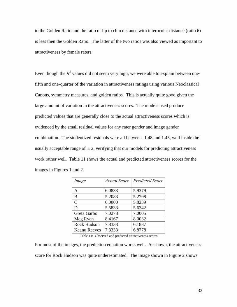
work rather well. Table 11 shows the actual and predicted attractiveness scores for the

images in Figures 1 and 2.

±

Image Actual Score Predicted Score

A 6.0833 5.9379 B 5.2083 5.2798 C 6.0000 5.8239 D 5.5833 5.6342 Greta Garbo 7.0278 7.0005 Meg Ryan 8.4167 8.0032 Rock Hudson 7.8333 6.1887 Keanu Reeves 7.3333 6.8778

Table 11: Observed and predicted attractiveness scores

For most of the images, the prediction equation works well. As shown, the attractiveness

score for Rock Hudson was quite underestimated. The image shown in Figure 2 shows

33

the face tilted and somewhat rotated which is a possible explanation as to why the model

underestimated his attractiveness.

5 Summary and Future Work

The goal of this study was to determine a predictive model for attractiveness based on

Neoclassical Canons, symmetry, and golden ratios. In contrast with much of the previous

work, our study used landmarks and geometry based means for computing symmetry and

had people rate actual faces instead of composite or altered faces. We also include both

images of the general population and images of known attractive faces. In addition we

identify both the gender of the rater and the image as to compare the ratings given to the

same and opposite genders, as suggested by Rhodes (2006). While men and women do

generally agree on overall attractiveness, male raters tend to give higher scores than their

female counterparts. In addition, we find that male and female raters use somewhat

different criteria for determining the attractiveness of a face. Female faces were rated

higher by both male and female raters which supports feminine traits being viewed as

attractive (Cunningham 1986, Cunningham et al. 1995, Rhodes 2006), but goes against

the idea that ratings reflect a sexual attractiveness toward faces of the opposite gender

(Cunningham et al. 1990). Our study on attractiveness is centered around the geometry

of the face using a set of landmarks. This facilitates understanding roles of individual

symmetric feature pairs and proportions in the attractiveness of a face. Our study is

consistent with Rhodes (2006) in concluding that smaller chins in females are more

attractive. We also find that smaller noses, a larger distance between the eyes, and

smaller widths of the mouth are desirable traits for females. Symmetry does not seem to

34

play as important a role in attractiveness as the proportions defined by the Neoclassical

Canons and golden ratios. This is demonstrated by the small proportion of symmetry

predictor variables, as compared to the proportions of canons and golden ratios that were

selected by the stepwise procedures to be included in the final models. Only three of the

eleven difference symmetry measures were in any of the four reduced models, while five

of six canons and six of seventeen golden ratios were included in at least one of the four

models.

While the results presented in this paper provide strong insights into the role that different

aspects of face geometry play in attractiveness, this research can be extended in many

different directions. Attractiveness is a complex aspect of a face and involves many other

issues, for example, Rhodes (2006) and others have studied the effects of averageness on

the attractiveness of faces. We are interested in exploring this issue using a landmark-

based approach rather than composite face images. A secondary motive for including the

images of famous people was to see if the perception of attractiveness changes over time.

Our famous images included two male and two female faces from each of the past eight

decades which would allow us to determine if a relationship with attractiveness exists due

to the age of the rater and the time period during which the person was famous.

6 References

Armstrong, J. 2004 The secret power of beauty: Why happiness is in the eye of the

beholder. London: Allen Lane.

35

Cunningham, M. R. 1986 Measuring the physical in physical attractiveness: quasi-

experiments on the sociobiology of female facial beauty. J. Personal. Soc. Psychol. 50,

925-935.

Cunningham, M. R., Barbee, A. P., & Pike, C. L. 1990 What do women want?

Facialmetric assessment of multiple motives in the perception of male facial physical

attractiveness. J. Personal. Soc. Psychol. 59, 61-72.

Cunningham, M. R., Roberts, A. R., Barbee, A. P, Druen, P. B., & Wu, C-H. 1995 “Their

ideas of beauty are, on the whole, the same as ours”: consistency and variability in the

crosscultural perception of female physical attractiveness. J. Personal. Soc. Psychol.

68, 261-279.

DeBruine, L. M. 2004 Facial resemblance increases the attractiveness of same-sex faces

more than other sex faces. Proc. R. Soc. Lond. Ser. B. Biol. Sci. 271, 2085-2090

Farkas, L.G. 1994 Anthropometry of the Head and Face. 2nd ed. Raven Press.

Farkas, L. G. & Munro, I. R. 1987 Anthropometric Facial Proportions in Medicine.

Illinois: Charles C. Thomas.

Farkas, L. G., Forrest, C. R., & Litsas, L. 2000 Revision of neoclassical facial canons in

young adult Afro-Americans. Aesthetic Plastic Surgery 24, 179-184.

Farkas, L. G., Hreczko, T. A., Kolar, J. C., & Munro, I. R. 1985 Vertical and horizontal

proportions of the face in young adult North American Caucasians: Revision of

neoclassical canons. Plastic and Reconstructive Surgery. 75, 328-337.

Grammer, K. & Thornhill, R. 1994 Human (Homosapiens) facial attractiveness and

sexual selection: the role of symmetry and averageness. J. Comp. Psychol. 108, 233-

242.

36

Kowner, R. 1996 Facial asymmetry and attractiveness judgement in developmental

perspective. J. Exp. Psychol. Hum. Percept. Perform. 22, 662-675.

Langlois, J. H., Kalakanis, L., Rubenstein, A. J., Larson, A., Hallam, M., & Smoot, M.

2000 Maxims or myths of beauty? A meta-analytic and theoretical review. Psychol.

Bull. 126, 390-423.

Langlois, J. H., & Roggman, L. A. 1990 Attractive faces are only average. Psychol. Sci.

1, 115-121.

Langlois, J. H., Roggman, L. A., & Musselman, L. 1994 What is average and what is not

average about attractive faces? Psychol. Sci. 5, 214-220.

Little, A. C., Burt, D. M., Penton-Voak, & Perrett, D.I. 2001 Self-perceived attractiveness

influences human female preferences for sexual dimorphism and symmetry in male

faces. Proc. R. Soc. Lond. Ser. B. Biol. Sci. 268, 39-44.

Little, A. C., & Hancock, P. J. B. 2002 The role of masculinity and distinctiveness in

judgments of human male facial attractiveness. Br. J. Psychol. 93, 451-464.

Little, A. C., & Jones, B. C. 2006 Attraction independent of detection suggests special

mechanisms for symmetry preferences in human face perception. Proc. R. Soc. Lond.

Ser. B. Biol. Sci. 273, 3093-3099.

Meisner, G. 2006 The human face. Available on the World Wide Web at

http://Goldennumber.net/face. Last Accessed on December 9, 2006.

Movie Actor Index. Available on the World Wide Web at

http://www.movieactors.com Last Accessed on December 20, 2006

37

Narain, D.L. 2003 The perfect face. Available on the World Wide Web at

http://cuip.uchicago.edu/~dlnarain/golden/activity8.htm. Last Accessed on December 9,

2006.

O’Toole, A. J., Price, T., Vetter, T., Bartlett, J. C., & Blanz, V. 1999 3D shape and 2D

surface textures of human faces: the role of “averages” in attractiveness and age. Image

Vis. Comput. 18, 9-19.

Penton-Voak, I. S., Jones, B. C., Little, A. C., Baker, S., Tiddeman, B., Burt, D. M., &

Perrett, D. I. 2001 Symmetry, sexual dimorphism in facial proportions and male facial

attractiveness. Proc. R. Soc. Lond. Ser. B. Biol. Sci. 268, 1617-1623.

Perrett, D. I., Burt, D. M., Penton-Voak, I. S., Lee, K. J., Rowland, D. A., & Edwards, R.

1999 Symmetry and human facial attractiveness. Evol. Hum. Behav. 20, 295-307.

Perrett, D. I., Lee, K. J., Penton-Voak, I., Rowland, D., Yoshikawa, S., Burt, D. M.,

Henzill, S. P., Castles, D. L., & Akamatsu, S. 1998 Effects of sexual dimorphism on

facial attractiveness. Nature. 394, 884-887.

Phillips, P. J., Moon, H., Rizvi, S. A., & Rauss, P. J. 2000 The FERET evaluation

methodology for face-recognition algorithms. IEEE Trans. Patt. Anal. & Mach. Intell.

22, 1090-1104.

Rhodes, G. 2006 The evolutionary psychology of facial beauty. Annu. Rev. Psychol. 57,

199-226.

Rhodes, G., Proffitt, F., Grady, J. M., & Sumich, A. 1998 Facial symmetry and the

perception of beauty. Psychol. Bull. Rev. 5, 659-669.

Rhodes, G., Sumich, A., & Byatt, G. 1999 Are average facial configurations attractive

only because of their symmetry? Psychol. Sci. 10, 52-58.

38

Rhodes, G., & Tremewan, T. 1996 Averageness, exaggeration, and facial attractiveness.

Psychol. Sci. 7, 105-110.

Samuels, C. A., Butterworth, G., Roberts, T., Graupner, L, & Hole, G. 1994 Facial

aesthetics—babies prefer attractiveness to symmetry. Perception 23, 823-831.

SAS Institute. 2003 Online Doc. Version 9. SAS Institute, Inc., Cary, NC.

Schabenberger, O. 2005 Introducing the GLIMMIX procedure for generalized linear

mixed models. Paper 196-30, SUGI 30. SAS Institute, Inc., Cary, NC.

Scheib, J. E., Gangestad, S. W., & Thornhill, R 1999 Facial attractiveness, symmetry and

cues of good genes. Proc. R. Soc. Lond. Ser. B. Biol. Sci. 266, 1913-1917.

Shi, J. Samal, A., & Marx, D. 2006 How effective are landmarks and their geometry for

face recognition? Computer Vision and Image Understanding 102, 117-133.

Smith, R. J. 1999 Statistics of sexual size dimorphism. Journal of Human Evolution 36,

423-459.

Swaddle, J. P., & Cuthill, I. C. 1995 Asymmetry and human facial attractiveness—

symmetry may not always be beautiful. Proc. R. Soc. Lond. Ser. B. Biol. Sci. 261, 111-

116.

39