Attention Discrimination in Retail Lending
30
Attention Discrimination in Retail Lending January 7, 2021 Bo Huang, Jiacui Li, Tse-Chun Lin, Mingzhu Tai, Yiyuan Zhou 1 Abstract Using proprietary retail loan screening data, we document that loan officers exhibit “attention discrimina- tion”. That is, discrimination happens at the earlier stage of information acquisition: loan officers exert less effort reviewing ex-ante unfavorable applicants and reject them at a higher rate. Further, when loan officers face stronger attention constraints when burdened by more applications, the degree of discrimination increases. This magnitude is significant: approval rate for the ex-ante disadvantaged applicants drops from 19.0% to 7.5% when officers are in the top decile of busyness. Overall, the results show that attention con- straints magnify discrimination. This has important implications on the strategy to reduce discrimination of decision makers. Keyword: attention allocation, attention constraint, statistical discrimination JEL Classification: D83, D91, G21 1 Introduction Since the seminal works of Phelps (1972) and Arrow (1972), it has been a crucial concern that decision makers may engage in statistical discrimination – that is, they rely on group attributes such as ethnicity or gender to make decisions when individual-level information is not available. This concern has been widely voiced in many contexts including decision making by judges in trials, recruitment by employers, voting in elections, college admission decisions, and so on. 2 In statistical discrimination, decision makers exhibit discrimination 1 Huang ([email protected]): School of Finance at Remin University of China. Li ([email protected]): David Eccles School of Business at University of Utah. Lin, Tai, and Zhou ([email protected], [email protected], [email protected]): School of Economics and Finance at University of Hong Kong. 2 Time Magazine (2002) cites a study that shows recruiters spend an average of six seconds on each resume. The Chronicle of Higher Education (2017) report that admission officers at the University of Pennsylvania spend four minutes on each initial read of each college application. 1
Transcript of Attention Discrimination in Retail Lending
Attention Discrimination in Retail Lending
January 7, 2021
Bo Huang, Jiacui Li, Tse-Chun Lin, Mingzhu Tai, Yiyuan Zhou1
Abstract
Using proprietary retail loan screening data, we document that loan officers exhibit “attention discrimina-
tion”. That is, discrimination happens at the earlier stage of information acquisition: loan officers exert
less effort reviewing ex-ante unfavorable applicants and reject them at a higher rate. Further, when loan
officers face stronger attention constraints when burdened by more applications, the degree of discrimination
increases. This magnitude is significant: approval rate for the ex-ante disadvantaged applicants drops from
19.0% to 7.5% when officers are in the top decile of busyness. Overall, the results show that attention con-
straints magnify discrimination. This has important implications on the strategy to reduce discrimination
of decision makers.
Keyword: attention allocation, attention constraint, statistical discrimination
JEL Classification: D83, D91, G21
1 Introduction
Since the seminal works of Phelps (1972) and Arrow (1972), it has been a crucial concern that decision makers
may engage in statistical discrimination – that is, they rely on group attributes such as ethnicity or gender
to make decisions when individual-level information is not available. This concern has been widely voiced in
many contexts including decision making by judges in trials, recruitment by employers, voting in elections,
college admission decisions, and so on.2 In statistical discrimination, decision makers exhibit discrimination
1Huang ([email protected]): School of Finance at Remin University of China. Li ([email protected]): DavidEccles School of Business at University of Utah. Lin, Tai, and Zhou ([email protected], [email protected], [email protected]):School of Economics and Finance at University of Hong Kong.
2Time Magazine (2002) cites a study that shows recruiters spend an average of six seconds on each resume. The Chronicleof Higher Education (2017) report that admission officers at the University of Pennsylvania spend four minutes on each initialread of each college application.
1
2
at the decision stage. However, when under attention constraints, they may also discriminate early on in
the information acquisition stage and pay less attention to the ex-ante disadvantaged groups. In a “cherry-
picking” situation where the default action without sufficient information is to reject, this discriminatory
attention allocation decision will magnify the role of pre-existing priors or preferences. (Bartos, Bauer,
Chytilova, and Matejka, 2016) call this mechanism “attention discrimination”.
The attention discrimination mechanism can be easily understood through an example. Consider the case
when referees are time-constrained in reviewing economics papers. When given infinite time, there are many
things referees can do to improve her judgement on the submissions such as scrutinizing each table, doing
thorough literature searches, and performing replications (which happens in some NBER discussions). That
is clearly unrealistic as referees face time constraints – they need to attend to their own work and life as well.
When faced with stronger time-constraints, referees may use their priors to guide how much effort to put in
each review. Such priors can include whether the referee personally finds the claims plausible, whether the
submission is written by well-established researchers and has been presented in notable conferences, etc. If a
paper scores negatively on all of these fronts – that is, it comes from an ex-ante disadvantaged group – then
the referee may decide to spend less effort scrutinizing the paper and hand out a quick rejection. Further,
the more time constrained is the reviewer, the more likely she will engage in such attention discrimination.
Even though attention discrimination is a natural phenomenon that may be reasonably expected to occur
in many decision making contexts, it is difficult to study empirically in real world application decision
processes.3 As noted by Gabaix (2019), “measuring attention is ... a hard task – we still have only a limited
number of papers that measure attention in field settings.” Further, to test the role of inattention, one also
needs plausibly exogenous shocks to attention constraints which is often lacking in field data. This paper
fills this gap by documenting attention discrimination using a large, detailed retail loan screening data set
from one of the largest Chinese banks. To the best of our knowledge, we are the first to document attention
discrimination using large-scale field data.
Our data contains the complete proprietary records of 92 officers deciding whether to approve approximately
146,000 retail loan applications over the span of a year (April 2013 to April 2014). We observe the screening
process in detail: for each application, we can trace which officer is it assigned to, what time is it assigned,
whether loan officers have conducted further due diligence, and when is the decision made. Loan officers do
face time constraints: the median review time on each application is only 18 minutes which includes both
reviewing and sometimes making further phone calls for due diligence. Because we observe all application
assignment and decision times, we also can measure how busy is each officer at a given time as a proxy for
the strength of attention constraints.
In our empirical exercise, we start by documenting the connection between attention allocation and approval
rate. Applications that receiver less attention – measured using less time spent in reviews or shorter officer-
written comments – are more likely to be rejected. The median time spent on eventually approved application
is 28 minutes but only 13 minutes – less than half – on rejected applications. 27% of rejections are reviewed
for less than 5 minutes before being rejected. Similarly, officers wrote a median of 57 Chinese characters of
comments on approved applications while only 6 characters on rejected applications.
3The seminal paper on attention discrimination, Bartos et al. (2016), ran field experiments through email advertisements inrental and labor markets.
3
Second, we find evidence that officers use simple signals to allocate their attention. In our data, some ap-
plicants are able to obtain official certificates for their income, employment, housing property, etc. Those
who can obtain such certificates often work for the public sector or larger companies, have more stable
employment, and have better credit history. Those who cannot obtain these certificates are ex-ante disad-
vantaged. Loan officers appear to make use of these in allocating attention. While many applicants with
such certificates are also not approved, they are usually rejected after longer review time and further due
diligence efforts by the officers. In contrast, the disadvantaged group without certificates are more likely to
be rejected after only a few minutes and without further due diligence.
To examine whether inattention exacerbates discrimination, we exploit variation in loan officer busyness,
measured by the number of decisions made by each officer on each day. We argue that officers are more
inattentive on busier days. Because an officer can endogenously choose to work faster or slower, her actual
busyness is endogenous, we also instrument this busyness measure using the number of applications assigned
to the officer on that day and the previous three days. As most officers strive to make decisions on most
assigned applications within a few days, this turns out to be a strong instrument and a good predictor of
actual busyness. Because the assignments are made by a central dispatcher algorithm that officers have no
control over, this is an arguably exogenous source of variation in busyness.
As predicted by the attention discrimination mechanism, when loan officers are busier (more inattentive),
they discriminate more against the disadvantaged group with fewer certificates. That is, those applications
are rejected with higher probability while the advantaged group is not effected (or even slightly positively
affected). This finding holds when we sort on within officer busyness and thus is not driven by officer-
specific preferences. The result is also robust to different definitions of ex-ante disadvantage and different
instruments for busyness. The degree of attention-based discrimination is economically significant. If an ex-
ante disadvantaged application happens to be decided upon when an officer is in the top decile of busyness,
the approval rate is only 7.5% as compared to 19.0% when in the bottom decile of busyness. That is, the
approval rate declines by more than half.
One may worry that our results are driven by endogenous changes in application quality on busy versus non-
busy days. Specifically, this alternative explanation requires that the true application quality gap between
the advantaged and disadvantaged groups increases when officers are busier. We alleviate this concern in two
steps. First, since we observe almost all of the application information, we can verify that all credit-relevant
application observables are balanced across busy versus non-busy periods. We also control for all relevant
observables in all our results. However, there remains the possibility that there are time-varying differences
in unobservables. To help alleviate this concern, we then construct a leave-one-out instrument using the
number of applications from other parts of the country that are assigned to the same loan officer. The idea
is as follows. The loan officers we observe work at the bank headquarter and screen applications from all
across the country. If a large number of applications from area A makes the loan officer busy, it can affect
her decision making on applications from area B. In this case, the quality of loans from area B is independent
to the application volume from area A that drives the busyness of the loan officer (after controlling for the
application volume in the local area). All our results are also robust to using this instrument.
We want to emphasize that attention discrimination behavior of loan officers may be either rational or behav-
ioral. From the rational perspective, attention discrimination can be understood as optimal behavior subject
4
to attention constraints. Because loan officers only approve a small fraction of applications, when busy, their
time is better spent on the learning about applicants from the “good groups” with higher average credit
quality. From the behavioral perspective, Kahneman (2011) argues that people are more likely to engage
in time-saving “System 1” heuristics when under time constraint. However, regardless of the interpretation,
the outcome is the same: inattention exacerbates discrimination.
This paper has two main contributions. First, we show that discrimination can happen early on in the
attention-allocation stage, in addition to the later decision-making stage. Second, our results indicate that
inattention magnifies discrimination. This has important implications for the staffing of decision making
institutions such as courts, the United States Patent and Trademark Office, college admission offices, and
so on. Conventionally, to combat discrimination, these institutions emphasize the use of anti-discrimination
training in order to help decision makers self-reflect and guard against their unconscious biases. However, our
findings indicate that discrimination may be an unavoidable consequence of attention constraints. Therefore,
these decision making institutions can alleviate discrimination simply by not being short-staffed.4
Discrimination in lending (e.g. Bartlett, Morse, Stanton, and Wallace (2019); Fuster, Goldsmith-Pinkham,
Ramadorai, and Walther (2020)) is considered a serious threat to fairness. In response to this, regulators
in the U.S. and around the world created various anti-discrimination legislation to combat discrimination
in financial practices. For example, The Equal Credit Opportunity Act (ECOA) prohibits creditors from
discriminating against credit applicants on the basis of race, color, religion, national origin, sex, marital
status, and age.5
This paper is closely related to the the seminal work of Bartos et al. (2016) that proposed the idea of
discrimination. Using a slightly different theoretical setting, Davies, Van Wesep, and Waters (2019) also
show that biases in decision-making can be magnified by endogenous information acquisition. This paper
is also related to studies on individual decision making behaviors in the credit market. For example, (?)
document that using soft information in lending decisions leads to worse loan quality when loan officers
are busy, and (Gao, Karolyi, and Pacelli, 2018) show that distracted loan officers are deficient in screening,
pricing, and monitoring. In addition, (Liao, Wang, Xiang, Yan, and Yang, 2020) find that individuals only
partially account for important credit information when making lending decisions under time pressure. Our
paper augments these studies by providing both theoretical foundations and empirical evidence for the role
of attention allocation in amplifying discrimination using step-by-step loan screening records.
The paper is organized as follows. Section 2 describes the data and relevant institutional details on the loan
screening process. Section 3 provides evidence that loan officer attention allocation matters for the eventual
decision. Section 4 shows that officers discriminate more when busier, and Section 5 concludes.
2 Data and Institutional Background
In this section, we describe the data and provide background information on the retail loan screening process.
4Many have argued that these institutions are short-staffed. For instance, Frakes and Wasserman (2017) argue that the U.S.patent office is short-staffed and that leads to the granting of invalid patents.
5See https://www.govinfo.gov/content/pkg/USCODE-2011-title15/html/USCODE-2011-title15-chap41-subchapIV.htm formore details.
5
The data we obtained is the complete internal records of loan screening from one of the largest Chinese
banks. The loan products are similar to standard regular retail financing in many markets, such as unsecured
personal term loans or secured home equity loans in the US. The data covers approximately 146,000 retail
loan applications screened by 92 officers over the course of April 2013 to April 2014. The median (mean)
loan amount is 60,000 (66,461) Chinese RMB which converts to 9,787 (10,841) US dollars. This is higher
than the Chinese GDP per capita of 7,073 USD in 2013. The average annual interest rate is 8.56% and
there are two possible maturities, with 28% of applications of 12 month maturity and the rest for 36 month
maturity. 34% of applications are approved and the rest are rejected. Summary statistics are presented in
Table 1.
2.1 The loan application screening process
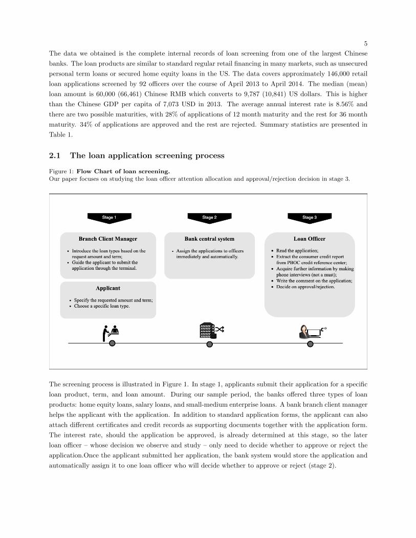
Figure 1: Flow Chart of loan screening.Our paper focuses on studying the loan officer attention allocation and approval/rejection decision in stage 3.
The screening process is illustrated in Figure 1. In stage 1, applicants submit their application for a specific
loan product, term, and loan amount. During our sample period, the banks offered three types of loan
products: home equity loans, salary loans, and small-medium enterprise loans. A bank branch client manager
helps the applicant with the application. In addition to standard application forms, the applicant can also
attach different certificates and credit records as supporting documents together with the application form.
The interest rate, should the application be approved, is already determined at this stage, so the later
loan officer – whose decision we observe and study – only need to decide whether to approve or reject the
application.Once the applicant submitted her application, the bank system would store the application and
automatically assign it to one loan officer who will decide whether to approve or reject (stage 2).
6
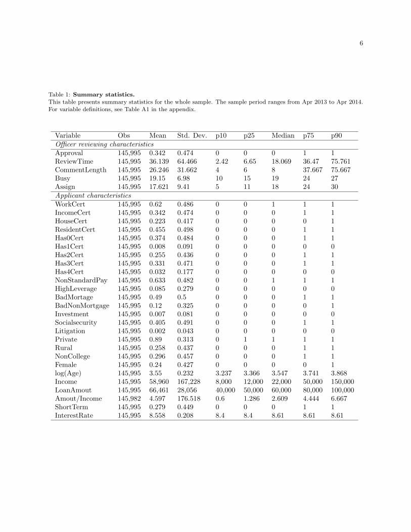
Table 1: Summary statistics.This table presents summary statistics for the whole sample. The sample period ranges from Apr 2013 to Apr 2014.For variable definitions, see Table A1 in the appendix.
Variable Obs Mean Std. Dev. p10 p25 Median p75 p90Officer reviewing characteristicsApproval 145,995 0.342 0.474 0 0 0 1 1ReviewTime 145,995 36.139 64.466 2.42 6.65 18.069 36.47 75.761CommentLength 145,995 26.246 31.662 4 6 8 37.667 75.667Busy 145,995 19.15 6.98 10 15 19 24 27Assign 145,995 17.621 9.41 5 11 18 24 30Applicant characteristicsWorkCert 145,995 0.62 0.486 0 0 1 1 1IncomeCert 145,995 0.342 0.474 0 0 0 1 1HouseCert 145,995 0.223 0.417 0 0 0 0 1ResidentCert 145,995 0.455 0.498 0 0 0 1 1Has0Cert 145,995 0.374 0.484 0 0 0 1 1Has1Cert 145,995 0.008 0.091 0 0 0 0 0Has2Cert 145,995 0.255 0.436 0 0 0 1 1Has3Cert 145,995 0.331 0.471 0 0 0 1 1Has4Cert 145,995 0.032 0.177 0 0 0 0 0NonStandardPay 145,995 0.633 0.482 0 0 1 1 1HighLeverage 145,995 0.085 0.279 0 0 0 0 0BadMortage 145,995 0.49 0.5 0 0 0 1 1BadNonMortgage 145,995 0.12 0.325 0 0 0 0 1Investment 145,995 0.007 0.081 0 0 0 0 0Socialsecurity 145,995 0.405 0.491 0 0 0 1 1Litigation 145,995 0.002 0.043 0 0 0 0 0Private 145,995 0.89 0.313 0 1 1 1 1Rural 145,995 0.258 0.437 0 0 0 1 1NonCollege 145,995 0.296 0.457 0 0 0 1 1Female 145,995 0.24 0.427 0 0 0 0 1log(Age) 145,995 3.55 0.232 3.237 3.366 3.547 3.741 3.868Income 145,995 58,960 167,228 8,000 12,000 22,000 50,000 150,000LoanAmout 145,995 66,461 28,056 40,000 50,000 60,000 80,000 100,000Amout/Income 145,982 4.597 176.518 0.6 1.286 2.609 4.444 6.667ShortTerm 145,995 0.279 0.449 0 0 0 1 1InterestRate 145,995 8.558 0.208 8.4 8.4 8.61 8.61 8.61
7
In stage 3, the loan officer can access the submitted application forms, all the supporting materials, and
a consumer credit report from the Chinese central bank’s credit reference center. The loan officers have
a number of levers they can pull to acquire information. They can screen the consumer credit report to
acquire demographic information (such as individual’s identification information, marital status, education
background, and working status), credit payment information (such as the detailed credit history on personal
loans, credit cards, mortgage loans, guarantee and other credit accounts), or seek other public records
obtained from public administration authorities (such as past civil or criminal records of the applicants ).
They can also call the applicant, the applicant’s employer and contacts, or anyone else they deem relevant.
The officers can also write internal comments on each application detailing their information acquisition and
rationale for the decision.
Our data contains detailed records of the application assignment in stage 2 and the loan officer decision in
stage 3, as well as all the submitted application information. Because our data ends in April 2014, vast
majority of approved loans have not yet matured so we do not observe the eventual default rate. Therefore,
we focus our attention on studying the approval/rejection decision of the loan officer. Having access to these
details allows us to peer into the often black box loan screening process.
3 Disadvantaged applications are at higher risk of attention dis-
crimination
We start by demonstrating that lower officer attention tends to lead to rejections. We then note that the
group of applicants without official certificates for their income, property, etc. are ex-ante disadvantaged.
Finally, we show that officers tend to be particularly inattentive to the disadvantaged group, often rejecting
those applications without extensive review or due diligence.
3.1 Attention is necessary for obtaining approval
An important premise of the attention discrimination mechanism is that, if an officer pays less attention to
an applicant, the default outcome is more likely a rejection. The reasoning is simple: the risk of accepting
unscrutinized applications is too high. This can be shown in a quick back-of-envelope exercise. Consider a
random loan application. The average interest rate in our sample is 8.6%. Even if the bank’s cost of capital
is the risk-free rate of 3.25% in our sample period, this means the bank can only make a cost-adjusted
annual return of 5.35% if the applicant does not default. In contrast, if the application defaults, assuming
a 40% recovery rate, the bank stands to loose 60%. Therefore, as long as the expected default rate of all
applications is higher than 3.25%3.25%+60% ≈ 5%, the default loan officer action without sufficient information
acquisition should be rejection.
We now examine whether attention appears to be associated with approval by using direct proxies of officer
attention. As noted by the survey paper of Gabaix (2019), it is hard to measure attention in field settings.
Luckily, with the complete administrative records of the internal loan screening process, we can construct
two reasonable proxies: the time spent on each application and the amount of comments written. The
former is measured as the number of minutes elapsed since the previous to the current decision. The latter
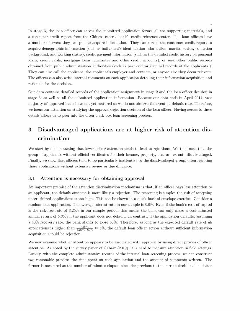
8Figure 2: Measures of attention allocation by loan officers.This figure shows the officer’s attention allocation in applications that are eventually approved or rejected. The leftpanel plots the distribution of the number of minutes the officer spent reviewing the application, measured as thetime gap between the officer’s previous and current decision. The right panel plots the density of the length of thecomments written by the officer one each application. The medians are marked with vertical dashed lines. To avoidhaving to plot the skewed right tail of the distributions, we trim those with review time longer than one hour andcomments longer than 100 characters.
is measured by the number of Chinese characters written by the officer as comments – a type of internal
memo – on the loan application.
Figure 2 plots the density of both attention variables for approved and rejected applications. Indeed, more
attention is paid on applications that are eventually approved. The median time spent on approved applica-
tions is 23.9 minutes and the median length of comments written is 52 characters, while the median time on
rejections is only 10.67 minutes and the median comment is only 6 characters. In fact, 27% of rejections are
done within 5 minutes, and vast majority of the rejection comments are uninformative, boilerplate comments
complaining about the credit worthiness of applicants.
3.2 Applicants without certificates are ex-ante disadvantaged
In addition to regular loan application material, some applicants are able to obtain official certificates for
their housing property, income, employment, and residence. Not everyone can obtain these certificates.
For instance, self-employed applicants or those working in free-lancing jobs are usually unable to obtain
employment or income certificates. We provide further details about these certificates in the Appendix.
We argue that applicants lacking these formal certificates are disadvantaged and thus likely to suffer from
lack of loan officer attention. We examine the validity of this argument in two ways. First, we demonstrate
9
that these applicants indeed have lower income and worse credit-related attributes. This is shown by the
regression results in Table 2. Applicants with certificates tend to have higher income, lower loan-to-income
ratio, lower ex-ante leverage, and lower chance of having bad mortgages payment histories. The relationship
is also monotone in the number of certificates that each applicant has as shown in columns 5, 10, 15, and 20.
Even though the certificates are correlated with loan characteristics, they clearly do not subsume the in-
formation in other characteristics as the association is not too high. This is shown in Figure ?? in the
Appendix.
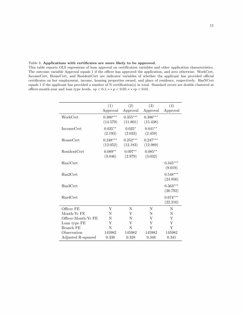
Second, we verify that applicants with more certificates are much more likely to have their loan application
approved. This is shown in Table 3. After controlling for a host of application-level observables, we find
that applicants with certificates are much more likely to be approved. In the main specification in column
3, we control for loan type, bank branch, and officer-year-month fixed effects. Columns 1 and 2 show that
the result is not sensitive to the choice of which fixed effects to include. Column 4 shows that approval rate
is increasing in the number of certificates that the applicant has.
3.3 Do officers use certificates to guide their attention allocation?
The discussion so far suggests that officers, when facing time constraints, may simply use the existence or lack
of certificates to guide their attention allocation across applications assigned to them. If so, we would expect
that applications with fewer or no certificates are more at risk of fast rejection without careful scrutiny.
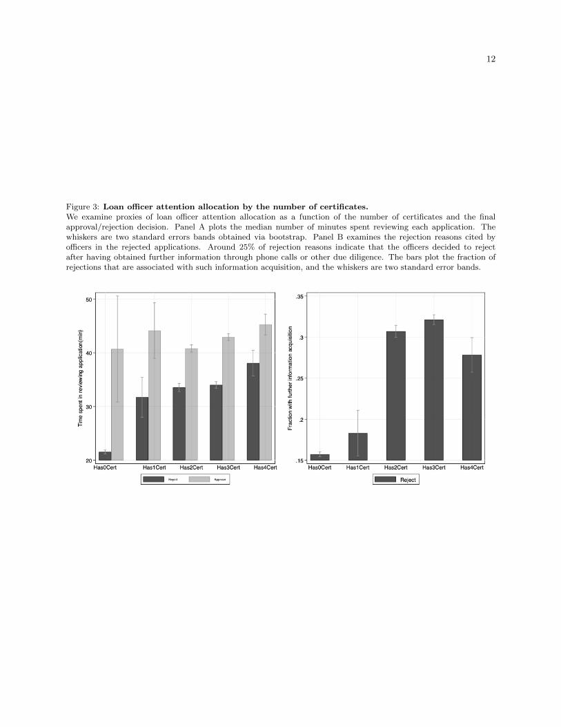
We indeed find evidence that officers use certificates to guide their attention allocation. Panel A of Figure 3
plots the median review time by officers for approved or rejected applications by the number of certificates.
The whiskers are two standard error bands.6 While the time spent on approved applications has little
dependence on the number of certificates, there is large difference in the time spent on rejected applications.
Officers only spend a median of 8.3 minutes before rejecting those without certificates but 21.7 minutes on
those with four certificates. This suggests that applications with no certificates are at high risk of being
rejected without careful review.
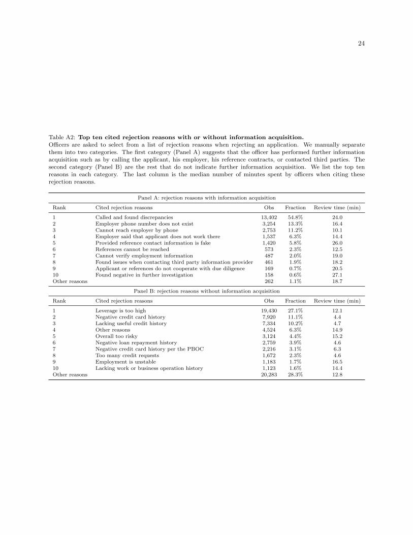
We also examine officer attention using what they cite as the reason for rejection. In the bank we study,
officers are asked to select from a list of standardized rejection reasons. While most cited rejection reasons
are boilerplate such as “bad credit quality”, “leverage is too high”, or even “other”, approximately 25%
of the rejection reasons indicate that the officer only rejected after having spent further effort acquiring
information by calling the applicant, contacting references, etc. We take the latter rejection reasons as an
indicator that the officer has attempted further due diligence. Indeed, officers spend a median of 20.7 minutes
when their rejection reasons indicate further due diligence and only 9.9 minutes when not. A list of most
common rejection reasons are listed in Table A2 in the appendix.
Panel B of Figure 3 plots the fraction of rejections with information acquisition. While this is admittedly a
noisy measure, the results show that applications with no certificates are more likely rejected without further
attempts of information acquisition by the officer. This is also consistent with the finding in Panel A which
indicates that such applications tend to be rejected rather quickly.
6We plot median instead of mean because the review time is heavily right skewed, but the results based on means arequalitatively similar.
10
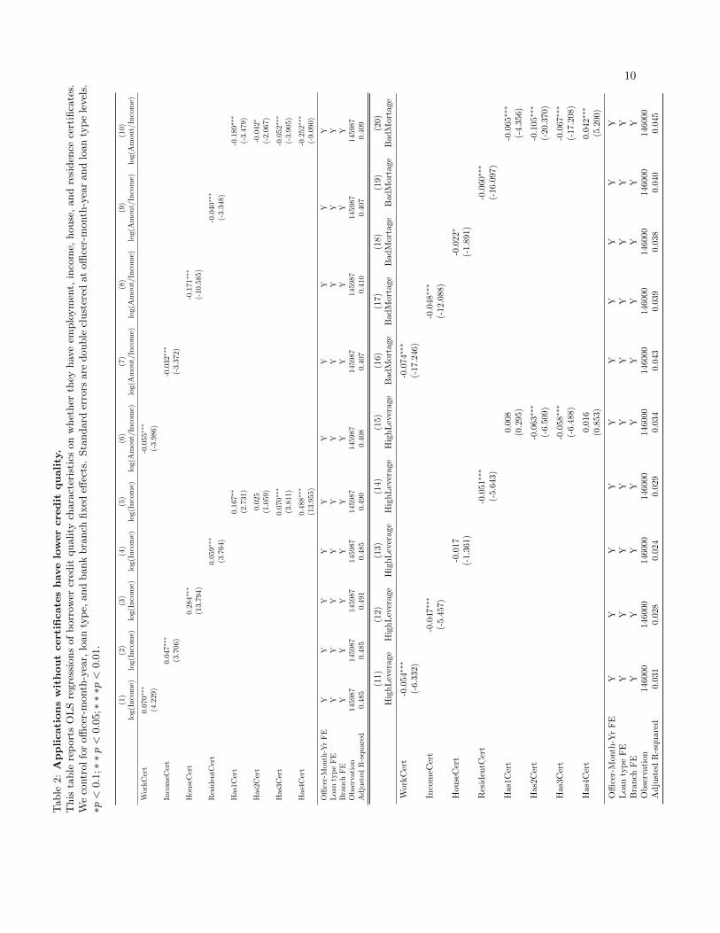
Table
2:
Applicati
ons
wit
hout
cert
ificate
shave
low
er
cre
dit
quality
.T
his
table
rep
ort
sO
LS
regre
ssio
ns
of
borr
ower
cred
itquality
chara
cter
isti
cson
whet
her
they
hav
eem
plo
ym
ent,
inco
me,
house
,and
resi
den
cece
rtifi
cate
s.W
eco
ntr
ol
for
offi
cer-
month
-yea
r,lo
an
typ
e,and
bank
bra
nch
fixed
effec
ts.
Sta
ndard
erro
rsare
double
clust
ered
at
offi
cer-
month
-yea
rand
loan
typ
ele
vel
s.∗p
<0.1
;∗∗p<
0.0
5;∗
∗∗p
<0.0
1.
(1)
(2)
(3)
(4)
(5)
(6)
(7)
(8)
(9)
(10)
log(I
nco
me)
log(I
nco
me)
log(I
nco
me)
log(I
nco
me)
log(I
nco
me)
log(A
mou
t/In
com
e)lo
g(A
mout/
Inco
me)
log(
Am
ou
t/In
com
e)lo
g(A
mou
t/In
com
e)lo
g(A
mou
t/In
com
e)
Wor
kC
ert
0.070
∗∗∗
-0.0
55∗∗
∗
(4.2
29)
(-3.
986)
Inco
meC
ert
0.0
47∗∗
∗-0
.032
∗∗∗
(3.7
06)
(-3.3
72)
Hou
seC
ert
0.28
4∗∗
∗-0
.171∗
∗∗
(13.7
94)
(-10
.585)
Res
iden
tCer
t0.0
59∗∗
∗-0
.040
∗∗∗
(3.7
64)
(-3.3
48)
Has
1C
ert
0.1
67∗
∗-0
.189
∗∗∗
(2.7
31)
(-3.4
79)
Has
2Cer
t0.0
25
-0.0
42∗
(1.0
59)
(-2.0
67)
Has
3Cer
t0.0
70∗∗
∗-0
.052
∗∗∗
(3.8
11)
(-3.9
05)
Has
4Cer
t0.4
88∗∗
∗-0
.252
∗∗∗
(13.9
55)
(-9.0
90)
Offi
cer-
Mon
th-Y
rF
EY
YY
YY
YY
YY
YL
oan
typ
eF
EY
YY
YY
YY
YY
YB
ran
chF
EY
YY
YY
YY
YY
YO
bse
rvat
ion
1459
87145
987
1459
87145987
145987
145
987
145
987
1459
87
1459
87
14598
7A
dju
sted
R-s
qu
are
d0.
485
0.485
0.49
10.4
85
0.4
90
0.40
80.
407
0.4
10
0.407
0.4
09
(11)
(12)
(13)
(14)
(15)
(16)
(17)
(18)
(19)
(20)
Hig
hL
ever
age
Hig
hL
ever
age
Hig
hL
ever
age
Hig
hL
ever
age
Hig
hL
ever
age
Bad
Mort
age
Bad
Mort
age
Bad
Mor
tage
Bad
Mor
tage
Bad
Mort
age
Wor
kC
ert
-0.0
54∗∗
∗-0
.074∗∗
∗
(-6.
332)
(-17.2
46)
Inco
meC
ert
-0.0
47∗∗
∗-0
.048
∗∗∗
(-5.
457)
(-12
.088
)
Hou
seC
ert
-0.0
17
-0.0
22∗
(-1.3
61)
(-1.8
91)
Res
iden
tCer
t-0
.051
∗∗∗
-0.0
60∗
∗∗
(-5.6
43)
(-16.
097
)
Has
1Cer
t0.0
08
-0.0
65∗∗
∗
(0.2
95)
(-4.
356)
Has
2Cer
t-0
.063∗∗
∗-0
.105∗
∗∗
(-6.5
09)
(-20.
370)
Has
3Cer
t-0
.058∗∗
∗-0
.067∗
∗∗
(-6.4
88)
(-17.
208)
Has
4Cer
t0.0
16
0.0
42∗∗
∗
(0.8
53)
(5.2
00)
Offi
cer-
Mon
th-Y
rF
EY
YY
YY
YY
YY
YL
oan
typ
eF
EY
YY
YY
YY
YY
YB
ran
chF
EY
YY
YY
YY
YY
YO
bse
rvat
ion
1460
00146
000
1460
00
146
000
146000
146000
1460
0014
600
014
600
0146
000
Ad
just
edR
-squ
ared
0.03
10.
028
0.0
24
0.02
90.0
34
0.0
43
0.0
390.
038
0.04
00.0
45
11
Table 3: Applications with certificates are more likely to be approved.This table reports OLS regressions of loan approval on certification variables and other application characteristics.The outcome variable Approval equals 1 if the officer has approved the application, and zero otherwise. WorkCert,IncomeCert, HouseCert, and ResidentCert are indicator variables of whether the applicant has provided officialcertificates on her employment, income, housing properties owned, and place of residence, respectively. HasNCertequals 1 if the applicant has provided a number of N certification(s) in total. Standard errors are double clustered atofficer-month-year and loan type levels. ∗p < 0.1; ∗ ∗ p < 0.05; ∗ ∗ ∗p < 0.01.
(1) (2) (3) (4)Approval Approval Approval Approval
WorkCert 0.380∗∗∗ 0.355∗∗∗ 0.386∗∗∗
(14.579) (11.801) (15.438)
IncomeCert 0.035∗∗ 0.035∗ 0.041∗∗
(2.193) (2.033) (2.459)
HouseCert 0.248∗∗∗ 0.252∗∗∗ 0.247∗∗∗
(12.052) (12.183) (12.989)
ResidentCert 0.089∗∗ 0.097∗∗ 0.085∗∗
(3.046) (2.979) (3.032)
Has1Cert 0.345∗∗∗
(9.019)
Has2Cert 0.548∗∗∗
(24.856)
Has3Cert 0.563∗∗∗
(26.792)
Has4Cert 0.674∗∗∗
(22.216)
Officer FE Y N N NMonth-Yr FE N Y N NOfficer-Month-Yr FE N N Y YLoan type FE Y Y Y YBranch FE N N Y YObservation 145982 145982 145982 145982Adjusted R-squared 0.338 0.328 0.348 0.341
12
Figure 3: Loan officer attention allocation by the number of certificates.We examine proxies of loan officer attention allocation as a function of the number of certificates and the finalapproval/rejection decision. Panel A plots the median number of minutes spent reviewing each application. Thewhiskers are two standard errors bands obtained via bootstrap. Panel B examines the rejection reasons cited byofficers in the rejected applications. Around 25% of rejection reasons indicate that the officers decided to rejectafter having obtained further information through phone calls or other due diligence. The bars plot the fraction ofrejections that are associated with such information acquisition, and the whiskers are two standard error bands.
13
4 Do officers discriminate more when they are busier?
We now test the key prediction of attention discrimination: do officers discriminate more when they are
busier?
4.1 Measuring officer busyness
We use several measures of officer busyness. First, we define busynessj,d as the number of decisions made
by officer j on day d. There is ample variation of busyness within officer. On average, an officer handles 24
loans in a top quintile busyness day and only 15 applications in a bottom quintile busyness day.
One obvious worry is that the actual number of decisions made by an officer is endogenous. For instance,
suppose applications with certain characteristics take longer to process, then the busyness of officer will
become negatively correlated with that characteristic. There is some evidence of such correlations in Panel
A of Table 5. Officers can also choose to work faster or slower based on their personal preferences.
Therefore, we want a cleaner measure of busyness that officers do not have control over. To do this, we
instrument the actual busyness using the number of applications assigned:
Busynessj,d = a+ b0 ·NumAssignmentj,d + b1 ·NumAssignmentj,d−1 + b2 ·NumAssignmentj,d−2 (1)
+ b3 ·NumAssignmentj,d−3 + Controls + εj,d (2)
We use up to 3 lagged work days because while some applications are not immediately decided, most
applications are decided within a few days of assignment. The results of this regression is shown in Table 4.
While our data provider does not disclose how exactly the assignment algorithm assign applications to
officers, we are informed that officers themselves have no influence on this assignment process. Thus, the
number of assignments is exogenous from the officer’s point of view. In Panel B of Table 5, we verify that
the predicted busyness measure is uncorrelated with all main observable loan characteristics.
Finally, one can also worry about correlation between unobservables and the number of assignments. To
partially address this concern, we also construct a loan-level leave-one-out instrument using the number of
applications from other parts of the country that are assigned to the same loan officer. The idea is that loan
officers at the headquarter office process loan applications from all across the country, and if a large number
of applications from area A makes the loan officer busy, it can affect her decision making on applications
from area B. In this case, the quality of loans from area B is independent to the application volume from
area A that drives the busyness of the loan officer (after controlling for the application volume in the local
area).7
4.2 Does discrimination increase when loan officer are busier?
We now examine whether loan officers discriminate more based on the certificates when busy.
7Panel C of Table 5 verifies that this measure is also not correlated with loan observables.
14
Table 4: Predicting loan officer busyness using assignments.This table reports the prediction of busyness by daily assignments. Busynessj,d is the total number of decisions madeby loan officer j on day d, while NumAssignmentj,d is the total number of assignments she received. Standard errorsare double clustered at officer-month-year and loan type levels.The regression is based on our officer-day level sample.∗p < 0.1; ∗ ∗ p < 0.05; ∗ ∗ ∗p < 0.01.
Dependent variable: Busynessj,d
(1) (2) (3) (4) (5) (6)
NumAssignmentj,d 0.520∗∗∗ 0.419∗∗∗ 0.393∗∗∗ 0.367∗∗∗ 0.332∗∗∗ 0.239∗∗∗
(11.412) (12.094) (12.355) (11.299) (10.405) (8.592)
NumAssignmentj,d−1 0.217∗∗∗ 0.174∗∗∗ 0.163∗∗∗ 0.142∗∗∗ 0.089∗∗∗
(6.030) (5.344) (5.514) (4.638) (3.527)
NumAssignmentj,d−2 0.125∗∗∗ 0.080∗∗∗ 0.064∗∗ 0.015(6.005) (3.946) (2.832) (0.799)
NumAssignmentj,d−3 0.140∗∗∗ 0.119∗∗∗ 0.054∗∗∗
(10.802) (8.715) (5.789)
Officer-Month-Yr FE N N N N N YLoan type FE N N N N Y YBranch FE N N N N N YObservation 9563 9563 9563 9563 9553 9494Adjusted R-squared 0.422 0.484 0.504 0.528 0.557 0.639
15
Table
5:
Exam
inin
gw
heth
er
applicati
on
obse
rvable
scorr
ela
tew
ith
offi
cer
busy
ness
measu
res.
Busy
nes
sis
defi
ned
as
the
num
ber
of
applica
tions
We
sort
the
sam
ple
into
dec
iles
base
don
act
ual
busy
nes
s,ass
ignm
ent-
pre
dic
ted
busy
nes
s,and
LO
O-
ass
ignm
ent-
pre
dic
ted
busy
nes
s,and
resu
lts
are
rep
ort
edin
Panel
sA
,B
,and
C.T
he
offi
cers
inth
elo
wes
t(h
ighes
t)dec
ile
are
the
least
(most
)busy
.Sta
ndard
erro
rsare
double
clust
ered
at
offi
cer-
month
-yea
rand
loan
typ
ele
vel
s.T
he
regre
ssio
nis
base
don
our
loan-l
evel
sam
ple
.∗p
<0.1
;∗∗p<
0.0
5;∗
∗∗p
<0.0
1.
Pan
elA
Act
ual
Bu
syn
ess
as
Reg
ress
or
(1)
(2)
(3)
(4)
(5)
(6)
(7)
(8)
(9)
(10)
Wor
kC
ert
Inco
meC
ert
Hou
seC
ert
Res
iden
tCer
tN
onSta
ndar
dP
ayH
igh
Lev
erag
eB
adM
orta
ge
BadN
onM
ort
gage
Inves
tmen
tS
oci
als
ecu
rity
Busy
Dec
ile
-12.
610∗
∗∗-7
.883
∗∗∗
-4.6
74∗∗
∗-9
.794
∗∗∗
8.03
5∗∗
∗1.
840∗
∗∗0.
516
-3.2
93∗∗
∗-0
.122
0.6
18
(-6.
706)
(-4.
945)
(-5.
573)
(-6.
226)
(5.5
29)
(4.0
90)
(0.6
27)
(-3.7
51)
(-0.8
47)
(0.7
41)
Offi
cer-
Mon
th-Y
rF
EY
YY
YY
YY
YY
YL
oan
typ
eF
EY
YY
YY
YY
YY
YB
ranch
FE
YY
YY
YY
YY
YY
Obse
rvat
ion
1460
0014
6000
1460
0014
600
014
6000
1460
0014
6000
146000
146000
146000
Adju
sted
R-s
quar
ed0.
092
0.31
70.
387
0.34
60.
302
0.023
0.03
80.0
62
0.0
10
0.0
82
(11)
(12)
(13)
(14)
(15)
(16)
(17)
(18)
(19)
(20)
Lit
igat
ion
Pri
vate
Rura
lN
on
Coll
ege
Fem
ale
log(A
ge)
log(I
nco
me)
log(
Am
ou
t/In
com
e)S
hort
Ter
mlo
g(In
tere
stra
te)
Bu
syD
ecil
e-0
.020
0.01
60.
494
0.8
52∗∗
-0.4
55
0.2
22-3
.399
2.483
0.515
-0.0
06
(-0.
206)
(0.0
36)
(0.7
94)
(2.5
47)
(-0.8
33)
(0.6
39)
(-1.6
16)
(1.3
11)
(1.6
12)
(-0.5
17)
Offi
cer-
Mon
th-Y
rF
EY
YY
YY
YY
YY
YL
oan
typ
eF
EY
YY
YY
YY
YY
YB
ran
chF
EY
YY
YY
YY
YY
YO
bse
rvat
ion
1460
0014
6000
146000
146000
146000
145995
145
987
1459
8714
6000
146
000
Ad
just
edR
-squ
ared
0.01
10.
068
0.051
0.1
170.
010
0.0
56
0.485
0.407
0.7
850.8
68
16
Pan
elB
Pre
dic
ted
Bu
syn
ess
as
Reg
ress
or
(1)
(2)
(3)
(4)
(5)
(6)
(7)
(8)
(9)
(10)
Wor
kC
ert
Inco
meC
ert
Hou
seC
ert
Res
iden
tCer
tN
onS
tan
dar
dP
ayH
igh
Lev
erag
eB
adM
ort
age
Bad
Non
Mort
gage
Inve
stm
ent
Soci
als
ecu
rity
Pre
dic
tBu
syD
ecil
e-1
.563
-1.0
71-0
.055
-1.7
75
1.32
00.6
48
0.58
2-0
.260
0.1
22
0.8
12
(-0.
597)
(-0.
576)
(-0.
057)
(-0.
830)
(0.7
79)
(1.2
34)
(0.7
72)
(-0.3
84)
(0.9
82)
(1.3
52)
Offi
cer-
Mon
th-Y
rF
EY
YY
YY
YY
YY
YL
oan
typ
eF
EY
YY
YY
YY
YY
YB
ran
chF
EY
YY
YY
YY
YY
YO
bse
rvat
ion
1460
0014
6000
1460
00
146
000
1460
0014
6000
146
000
146000
146000
146000
Ad
just
edR
-squ
ared
0.08
90.
316
0.38
70.3
450.
301
0.023
0.0
380.0
61
0.0
10
0.0
82
(11)
(12)
(13)
(14)
(15)
(16)
(17)
(18)
(19)
(20)
Lit
igat
ion
Pri
vate
Rura
lN
on
Coll
ege
Fem
ale
log(A
ge)
log(I
nco
me)
log(A
mou
t/In
com
e)S
hort
Ter
mlo
g(I
nte
rest
rate
)
Pre
dic
tBu
syD
ecil
e-0
.070
-0.2
53-0
.762
0.2
59
0.1
11
-0.1
17
-0.0
76
0.3
08
0.1
06
-0.0
15
(-0.
690)
(-0.
554)
(-1.
117)
(0.6
18)
(0.2
50)
(-0.3
51)
(-0.0
50)
(0.2
33)
(0.4
66)
(-1.2
17)
Offi
cer-
Mon
th-Y
rF
EY
YY
YY
YY
YY
YL
oan
typ
eF
EY
YY
YY
YY
YY
YB
ran
chF
EY
YY
YY
YY
YY
YO
bse
rvat
ion
1460
0014
6000
14600
01460
00
1460
00
145995
14598
714598
7146000
146000
Ad
just
edR
-squ
ared
0.01
10.
068
0.0
510.1
17
0.0
10
0.0
56
0.4
85
0.407
0.7
85
0.8
68
Pan
elC
Sp
ati
al
Lea
ve-
On
e-O
ut
Pre
dic
ted
Bu
syn
ess
as
Reg
ress
or
(1)
(2)
(3)
(4)
(5)
(6)
(7)
(8)
(9)
(10)
Wor
kC
ert
Inco
meC
ert
Hou
seC
ert
Res
iden
tCer
tN
onSta
ndard
Pay
Hig
hL
ever
age
Bad
Mort
age
BadN
onM
ort
gage
Inve
stm
ent
Soci
als
ecuri
ty
Pre
dic
tBusy
Dec
ile
0.13
5-0
.071
0.440
-0.2
63-0
.131
0.11
1-0
.066
-0.0
90
0.0
25
0.2
95
(0.0
54)
(-0.
043)
(0.4
39)
(-0.
129)
(-0.
081)
(0.3
15)
(-0.0
99)
(-0.1
30)
(0.2
14)
(0.5
33)
Con
trol
for
loca
lbusy
nes
sY
YY
YY
YY
YY
YO
ffice
r-M
onth
-Yr
FE
YY
YY
YY
YY
YY
Loa
nty
pe
FE
YY
YY
YY
YY
YY
Bra
nch
FE
YY
YY
YY
YY
YY
Obse
rvat
ion
1460
0014
6000
1460
00
1460
0014
600
014
6000
1460
00146000
146000
146000
Adju
sted
R-s
quar
ed0.
089
0.31
60.
387
0.34
50.
301
0.02
30.0
38
0.0
61
0.0
10
0.0
82
(11)
(12)
(13)
(14)
(15)
(16)
(17)
(18)
(19)
(20)
Lit
igat
ion
Pri
vate
Rura
lN
on
Coll
ege
Fem
ale
log(
Age
)lo
g(I
nco
me)
log(A
mou
t/In
com
e)S
hor
tTer
mlo
g(In
tere
stra
te)
Pre
dic
tBu
syD
ecil
e-0
.075
-0.2
92
-0.8
840.
002
-0.6
50-0
.103
0.47
90.
120
0.248
-0.0
19(-
0.69
5)(-
0.64
3)
(-1.3
45)
(0.0
03)
(-1.
617)
(-0.2
92)
(0.2
75)
(0.0
80)
(0.7
63)
(-1.
257)
Con
trol
for
loca
lb
usy
nes
sY
YY
YY
YY
YY
YO
ffice
r-M
onth
-Yr
FE
YY
YY
YY
YY
YY
Loa
nty
pe
FE
YY
YY
YY
YY
YY
Bra
nch
FE
YY
YY
YY
YY
YY
Ob
serv
atio
n14
6000
1460
00
14600
0146
000
14600
0145
995
145
987
1459
8714
6000
1460
00
Ad
just
edR
-squ
ared
0.01
10.
068
0.0
510.1
170.
010
0.05
60.4
85
0.40
70.
785
0.8
68
17
To capture the extent to which the four certificates collectively affect loan officer decisions, we construct a
single-dimension measure that reflect the applicant’s ex-ante advantageousness perceived by the loan officer
based on the existence of those four certificates. This measure is estimated by regressing the actual approval
outcome on the four certificate indicators and then computing the predicted value of the outcome. The
estimation is shown in Table 3. We call the certificates-predicted approval rate, which is continuous, as
AdvantageContinuous. For simplicity of plotting, we also split applications into halves by this measure and
create an indicator variable AdvantageDiscrete which equals 1 for applications in the top 50% of Advantage-
Continuous.
To exploit variation in busyness, we split the sample into deciles based on the three busyness measures.
We then estimate the impact of being in the ex-ante advantaged group on approval rate interacted with
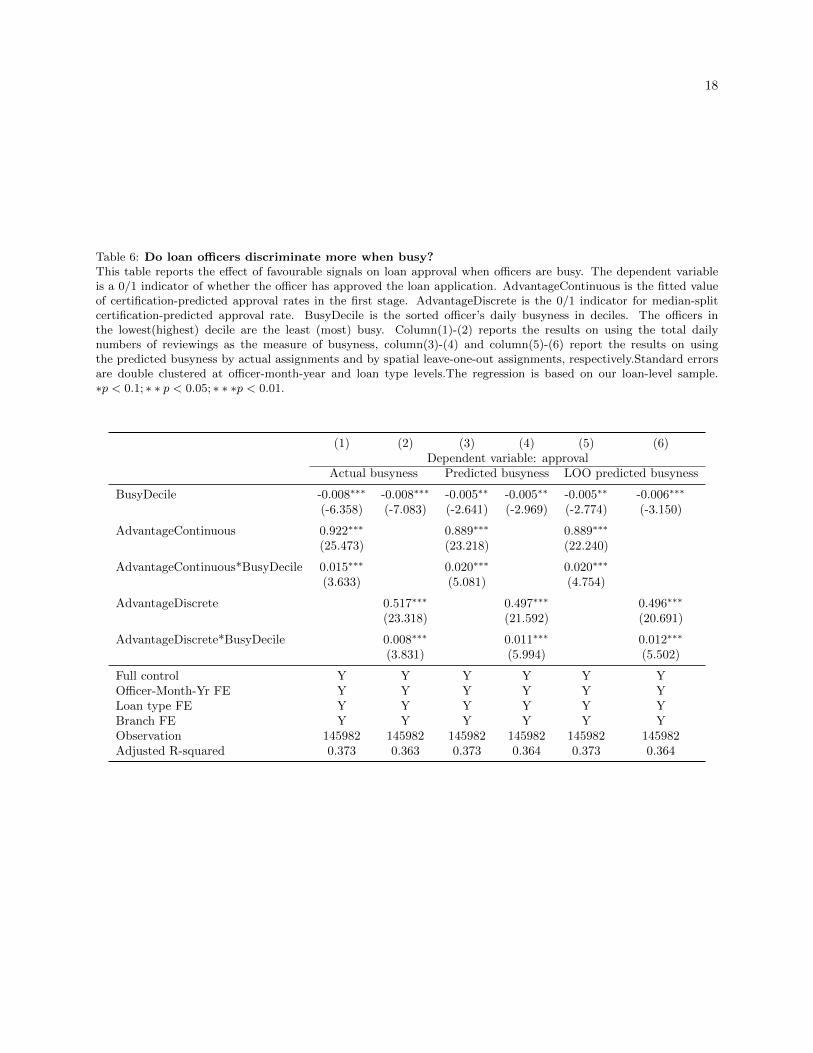
busyness. Table 6 reports the results. As predicted, when officers are busier, their decision depends more
heavily on whether the application is from the more ex-ante advantage group. Regardless of the busyness
measure used, the coefficient of approval rate on AdvantageDiscrete increases by 8% to 12% when busyness
goes from the lowest to the highest decile (columns 2, 4, and 6). This effect is economically large as the
overall approval rate is only 34%.
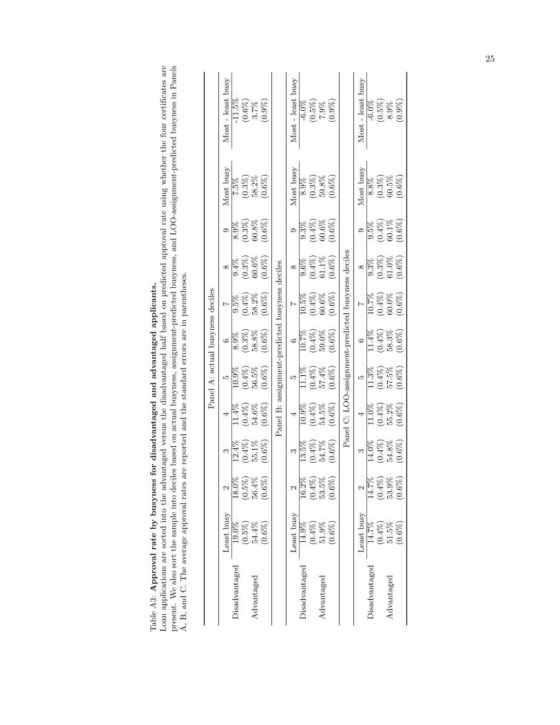
How large are the effects? To get an intuitive sense, Figure 4 plots the average approval rate of advantaged
and disadvantaged applicants in the ten deciles of busyness. The disadvantaged group has an approval rate
of 14.7% to 19.0% in the least busy decile but that declines to around half – 7.5% to 8.9% – in the most busy
decile. In contrast, the advantaged group enjoys some increase in approval rate. The numbers are reported
in Table A3 in the appendix.
In an ideal world, applications should only be judged based on their creditworthiness. However, in our
sample, the actual outcome also depends on the extraneous factor of whether the officer happens to be busy
or not when processing the application.
4.3 Robustness
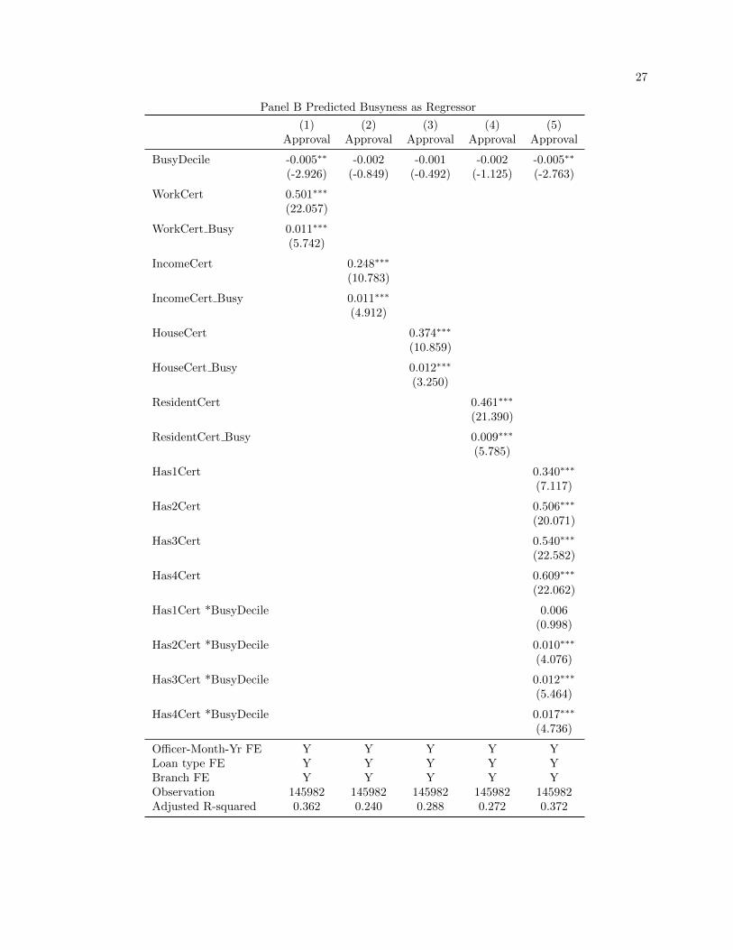
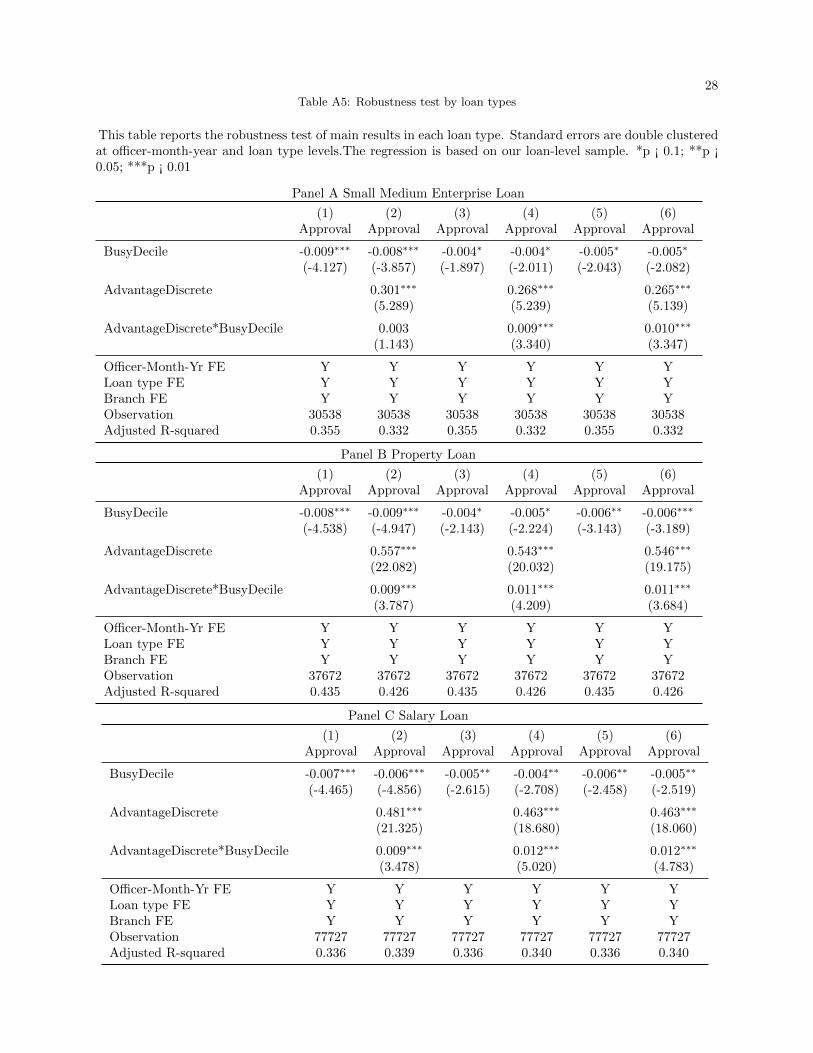
One may be concerned that our results depend on the specific way we define advantage and disadvantage ap-
plicants. We now verify that the result also holds when we separately examining each of the four certificates,
as shown in Table A4. To conserve space, we only report results using the LOO-assignment-predicted-
busyness as the results using the other two measures, reported in the appendix, are similar. For each of the
four certificates, their impact on approval rate increases when the loan officer is busier. Further, column 5
shows that the interaction effect increases with the number of certificates.
The effect is also relatively monotone in the degree of busyness. To test this, we replace the busyness Decile
in the earlier regression by indicators:
Approvali = a+
10∑k=1
bk ·AdvantageDiscrete · Ibusyness decile k + Controlsi + εi
and plot the coefficients {b1, ..., b10} in Panel A of Figure 5 with two standard error bands. For the lowest
busyness decile, the advantaged applications are accepted with approximately 50% higher probability, a
18
Table 6: Do loan officers discriminate more when busy?This table reports the effect of favourable signals on loan approval when officers are busy. The dependent variableis a 0/1 indicator of whether the officer has approved the loan application. AdvantageContinuous is the fitted valueof certification-predicted approval rates in the first stage. AdvantageDiscrete is the 0/1 indicator for median-splitcertification-predicted approval rate. BusyDecile is the sorted officer’s daily busyness in deciles. The officers inthe lowest(highest) decile are the least (most) busy. Column(1)-(2) reports the results on using the total dailynumbers of reviewings as the measure of busyness, column(3)-(4) and column(5)-(6) report the results on usingthe predicted busyness by actual assignments and by spatial leave-one-out assignments, respectively.Standard errorsare double clustered at officer-month-year and loan type levels.The regression is based on our loan-level sample.∗p < 0.1; ∗ ∗ p < 0.05; ∗ ∗ ∗p < 0.01.
(1) (2) (3) (4) (5) (6)Dependent variable: approval
Actual busyness Predicted busyness LOO predicted busyness
BusyDecile -0.008∗∗∗ -0.008∗∗∗ -0.005∗∗ -0.005∗∗ -0.005∗∗ -0.006∗∗∗
(-6.358) (-7.083) (-2.641) (-2.969) (-2.774) (-3.150)
AdvantageContinuous 0.922∗∗∗ 0.889∗∗∗ 0.889∗∗∗
(25.473) (23.218) (22.240)
AdvantageContinuous*BusyDecile 0.015∗∗∗ 0.020∗∗∗ 0.020∗∗∗
(3.633) (5.081) (4.754)
AdvantageDiscrete 0.517∗∗∗ 0.497∗∗∗ 0.496∗∗∗
(23.318) (21.592) (20.691)
AdvantageDiscrete*BusyDecile 0.008∗∗∗ 0.011∗∗∗ 0.012∗∗∗
(3.831) (5.994) (5.502)
Full control Y Y Y Y Y YOfficer-Month-Yr FE Y Y Y Y Y YLoan type FE Y Y Y Y Y YBranch FE Y Y Y Y Y YObservation 145982 145982 145982 145982 145982 145982Adjusted R-squared 0.373 0.363 0.373 0.364 0.373 0.364
19
Figure 4: Approval rate by busyness for disadvantaged and advantaged applicants.Loan applications are sorted into the advantaged versus the disadvantaged half based on predicted approval rate usingwhether the four certificates are present. We also sort the sample into deciles based on actual busyness, assignment-predicted busyness, and LOO-assignment-predicted busyness in Panels A, B, and C.
(a) Sorting on actual busyness (b) Sorting on predicted busyness
(c) Sorting on LOO-predicted busyness
20
number that increases to around 60% in the top busyness decile regardless of the busyness measure used.
In Panel B, we repeat the same exercise by only each of the four individual certificates and the results are
qualitatively similar. To conserve space, in Panel B, we only report results using the LOO busyness measure
and report the qualitatively similar results using other busyness measures in the appendix. Finally, in Table
A5, we also verify that our findings are robust in each of the three types of loans.
5 Conclusion
Traditionally, researchers focus on preference-based and statistical-discrimination of decision makers. In this
paper, we call attention to “attention discrimination”. That is, when acting under attention constraints,
decision makers may choose to pay less attention to ex-ante disadvantaged applicants and exert less effort
acquiring information about them. In settings where the default action is to reject, this leads to higher
rejection rates for those disadvantaged applicants.
This paper is the first to document attention discrimination in large-scale field data. Using the proprietary
retail loan screening records of a large Chinese bank, we show that loan officers allocate less attention to
reviewing applicants who cannot obtain official certificates for their income, property, etc. Those disadvan-
taged applicants are much more likely to be summarily rejected only after a few minutes of review. Further,
when loan officers are busy and overwhelmed by workload, such discrimination increases. The effect is
economically significant: if a disadvantaged application is processed when officers are in the top decile of
busyness, its approval probability shrinks from 19% to 7.5% – a three-fifths reduction.
Our findings have important implications for designing policies to combat discrimination. Since discrimina-
tion is the unintentional byproduct of busyness, it is important for the decision makers to not be overwhelmed
by workload. Unfortunately, this is often the case for court judges, USPTO patent examiners, etc. Then
more these institutions are short-staffed, the more it may be unavoidable for them to exhibit discriminatory
propensities.
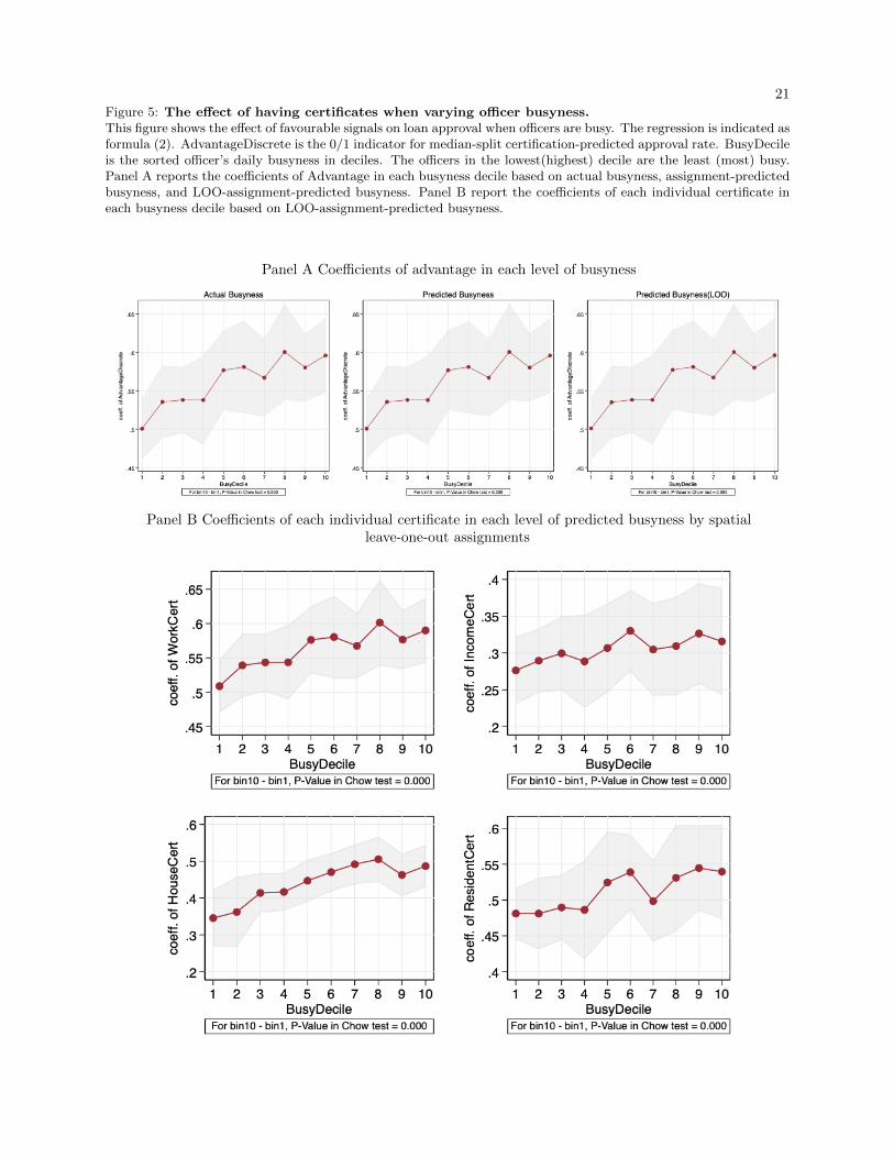
21Figure 5: The effect of having certificates when varying officer busyness.This figure shows the effect of favourable signals on loan approval when officers are busy. The regression is indicated asformula (2). AdvantageDiscrete is the 0/1 indicator for median-split certification-predicted approval rate. BusyDecileis the sorted officer’s daily busyness in deciles. The officers in the lowest(highest) decile are the least (most) busy.Panel A reports the coefficients of Advantage in each busyness decile based on actual busyness, assignment-predictedbusyness, and LOO-assignment-predicted busyness. Panel B report the coefficients of each individual certificate ineach busyness decile based on LOO-assignment-predicted busyness.
Panel A Coefficients of advantage in each level of busyness
Panel B Coefficients of each individual certificate in each level of predicted busyness by spatialleave-one-out assignments
22
References
Arrow, Kenneth J, 1972, Models of job discrimination, Racial discrimination in economic life 83.
Bartlett, Robert, Adair Morse, Richard Stanton, and Nancy Wallace, 2019, Consumer-lending discrimination
in the fintech era, Technical report, National Bureau of Economic Research.
Bartos, Vojtech, Michal Bauer, Julie Chytilova, and Filip Matejka, 2016, Attention discrimination: Theory
and field experiments with monitoring information acquisition, American Economic Review 106, 1437–75.
Davies, Shaun, Edward Dickersin Van Wesep, and Brian Waters, 2019, On the magnification of small biases
in decision-making, Available at SSRN 3407651 .
Frakes, Michael D, and Melissa F Wasserman, 2017, Is the time allocated to review patent applications induc-
ing examiners to grant invalid patents? evidence from microlevel application data, Review of Economics
and Statistics 99, 550–563.
Fuster, Andreas, Paul Goldsmith-Pinkham, Tarun Ramadorai, and Ansgar Walther, 2020, Predictably un-
equal? the effects of machine learning on credit markets .
Gabaix, Xavier, 2019, Behavioral inattention, Handbook of Behavioral Economics: Applications and Foun-
dations 1 2, 261–343.
Gao, Janet, Stephen A Karolyi, and Joseph Pacelli, 2018, Screening and monitoring by inattentive corporate
loan officers, Technical report, Working Paper.
Kahneman, Daniel, 2011, Thinking, fast and slow (Macmillan).
Liao, Li, Zhengwei Wang, Jia Xiang, Hongjun Yan, and Jun Yang, 2020, User interface and firsthand
experience in retail investing, The Review of Financial Studies .
Phelps, Edmund S, 1972, The statistical theory of racism and sexism, The american economic review 62,
659–661.
The Chronicle of Higher Education, 2017, Working smarter, not harder, in admissions, Online article by
Eric Hoover (March 12, 2017) .
Time Magazine, 2002, How to make your resume last longer than 6 seconds, Online article by Josh Sanburn
(April 13, 2012) .
23
APPENDIX
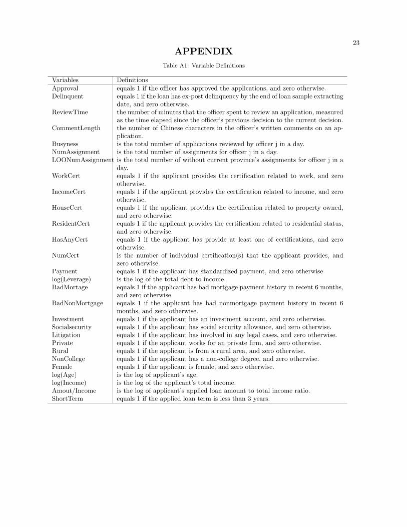
Table A1: Variable Definitions
Variables DefinitionsApproval equals 1 if the officer has approved the applications, and zero otherwise.Delinquent equals 1 if the loan has ex-post delinquency by the end of loan sample extracting
date, and zero otherwise.ReviewTime the number of minutes that the officer spent to review an application, measured
as the time elapsed since the officer’s previous decision to the current decision.CommentLength the number of Chinese characters in the officer’s written comments on an ap-
plication.Busyness is the total number of applications reviewed by officer j in a day.NumAssignment is the total number of assignments for officer j in a day.LOONumAssignment is the total number of without current province’s assignments for officer j in a
day.WorkCert equals 1 if the applicant provides the certification related to work, and zero
otherwise.IncomeCert equals 1 if the applicant provides the certification related to income, and zero
otherwise.HouseCert equals 1 if the applicant provides the certification related to property owned,
and zero otherwise.ResidentCert equals 1 if the applicant provides the certification related to residential status,
and zero otherwise.HasAnyCert equals 1 if the applicant has provide at least one of certifications, and zero
otherwise.NumCert is the number of individual certification(s) that the applicant provides, and
zero otherwise.Payment equals 1 if the applicant has standardized payment, and zero otherwise.log(Leverage) is the log of the total debt to income.BadMortage equals 1 if the applicant has bad mortgage payment history in recent 6 months,
and zero otherwise.BadNonMortgage equals 1 if the applicant has bad nonmortgage payment history in recent 6
months, and zero otherwise.Investment equals 1 if the applicant has an investment account, and zero otherwise.Socialsecurity equals 1 if the applicant has social security allowance, and zero otherwise.Litigation equals 1 if the applicant has involved in any legal cases, and zero otherwise.Private equals 1 if the applicant works for an private firm, and zero otherwise.Rural equals 1 if the applicant is from a rural area, and zero otherwise.NonCollege equals 1 if the applicant has a non-college degree, and zero otherwise.Female equals 1 if the applicant is female, and zero otherwise.log(Age) is the log of applicant’s age.log(Income) is the log of the applicant’s total income.Amout/Income is the log of applicant’s applied loan amount to total income ratio.ShortTerm equals 1 if the applied loan term is less than 3 years.
24
Table A2: Top ten cited rejection reasons with or without information acquisition.Officers are asked to select from a list of rejection reasons when rejecting an application. We manually separatethem into two categories. The first category (Panel A) suggests that the officer has performed further informationacquisition such as by calling the applicant, his employer, his reference contracts, or contacted third parties. Thesecond category (Panel B) are the rest that do not indicate further information acquisition. We list the top tenreasons in each category. The last column is the median number of minutes spent by officers when citing theserejection reasons.
Panel A: rejection reasons with information acquisition
Rank Cited rejection reasons Obs Fraction Review time (min)
1 Called and found discrepancies 13,402 54.8% 24.02 Employer phone number does not exist 3,254 13.3% 16.43 Cannot reach employer by phone 2,753 11.2% 10.14 Employer said that applicant does not work there 1,537 6.3% 14.45 Provided reference contact information is fake 1,420 5.8% 26.06 References cannot be reached 573 2.3% 12.57 Cannot verify employment information 487 2.0% 19.08 Found issues when contacting third party information provider 461 1.9% 18.29 Applicant or references do not cooperate with due diligence 169 0.7% 20.510 Found negative in further investigation 158 0.6% 27.1Other reasons 262 1.1% 18.7
Panel B: rejection reasons without information acquisition
Rank Cited rejection reasons Obs Fraction Review time (min)
1 Leverage is too high 19,430 27.1% 12.12 Negative credit card history 7,920 11.1% 4.43 Lacking useful credit history 7,334 10.2% 4.74 Other reasons 4,524 6.3% 14.95 Overall too risky 3,124 4.4% 15.26 Negative loan repayment history 2,759 3.9% 4.67 Negative credit card history per the PBOC 2,216 3.1% 6.38 Too many credit requests 1,672 2.3% 4.69 Employment is unstable 1,183 1.7% 16.510 Lacking work or business operation history 1,123 1.6% 14.4Other reasons 20,283 28.3% 12.8
25
Table
A3:
Appro
val
rate
by
busy
ness
for
dis
advanta
ged
and
advanta
ged
applicants
.L
oan
applica
tions
are
sort
edin
toth
eadva
nta
ged
ver
sus
the
dis
adva
nta
ged
half
base
don
pre
dic
ted
appro
val
rate
usi
ng
whet
her
the
four
cert
ifica
tes
are
pre
sent.
We
als
oso
rtth
esa
mple
into
dec
iles
base
don
act
ual
busy
nes
s,ass
ignm
ent-
pre
dic
ted
busy
nes
s,and
LO
O-a
ssig
nm
ent-
pre
dic
ted
busy
nes
sin
Panel
sA
,B
,and
C.
The
aver
age
appro
val
rate
sare
rep
ort
edand
the
standard
erro
rsare
inpare
nth
eses
.
Pan
elA
:act
ual
bu
syn
ess
dec
iles
Lea
stb
usy
23
45
67
89
Most
bu
syM
ost
-le
ast
bu
syD
isad
vanta
ged
19.0
%18.0
%12.4
%11.4
%10.9
%8.9
%9.5
%9.4
%8.9
%7.5
%-1
1.5
%(0
.5%
)(0
.5%
)(0
.4%
)(0
.4%
)(0
.4%
)(0
.3%
)(0
.4%
)(0
.3%
)(0
.3%
)(0
.3%
)(0
.6%
)A
dvanta
ged
54.4
%56.4
%55.1
%54.6
%56.5
%58.8
%58.2
%60.6
%60.8
%58.2
%3.7
%(0
.6%
)(0
.6%
)(0
.6%
)(0
.6%
)(0
.6%
)(0
.6%
)(0
.6%
)(0
.6%
)(0
.6%
)(0
.6%
)(0
.9%
)
Pan
elB
:ass
ign
men
t-p
red
icte
db
usy
nes
sd
eciles
Lea
stb
usy
23
45
67
89
Most
bu
syM
ost
-le
ast
bu
syD
isad
vanta
ged
14.9
%16.2
%13.5
%10.9
%11.1
%10.7
%10.5
%9.6
%9.3
%8.9
%-6
.0%
(0.4
%)
(0.4
%)
(0.4
%)
(0.4
%)
(0.4
%)
(0.4
%)
(0.4
%)
(0.4
%)
(0.4
%)
(0.3
%)
(0.5
%)
Ad
vanta
ged
51.9
%53.5
%54.7
%54.5
%57.4
%59.0
%60.6
%61.1
%60.6
%59.8
%7.9
%(0
.6%
)(0
.6%
)(0
.6%
)(0
.6%
)(0
.6%
)(0
.6%
)(0
.6%
)(0
.6%
)(0
.6%
)(0
.6%
)(0
.9%
)
Pan
elC
:L
OO
-ass
ign
men
t-p
red
icte
db
usy
nes
sd
eciles
Lea
stb
usy
23
45
67
89
Most
bu
syM
ost
-le
ast
bu
syD
isad
vanta
ged
14.7
%14.7
%14.0
%11.0
%11.3
%11.4
%10.7
%9.3
%9.5
%8.8
%-6
.0%
(0.4
%)
(0.4
%)
(0.4
%)
(0.4
%)
(0.4
%)
(0.4
%)
(0.4
%)
(0.3
%)
(0.4
%)
(0.3
%)
(0.5
%)
Ad
vanta
ged
51.5
%53.9
%54.8
%55.2
%57.5
%58.3
%60.0
%61.0
%60.1
%60.5
%8.9
%(0
.6%
)(0
.6%
)(0
.6%
)(0
.6%
)(0
.6%
)(0
.6%
)(0
.6%
)(0
.6%
)(0
.6%
)(0
.6%
)(0
.9%
)
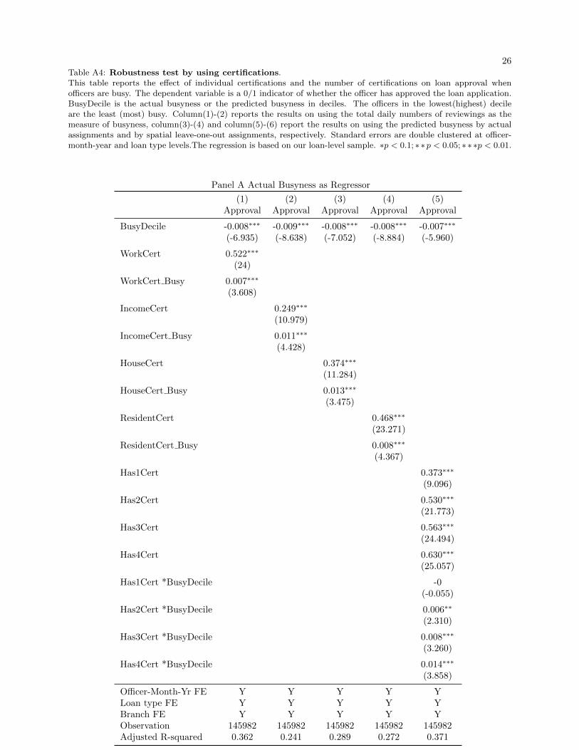
26Table A4: Robustness test by using certifications.This table reports the effect of individual certifications and the number of certifications on loan approval whenofficers are busy. The dependent variable is a 0/1 indicator of whether the officer has approved the loan application.BusyDecile is the actual busyness or the predicted busyness in deciles. The officers in the lowest(highest) decileare the least (most) busy. Column(1)-(2) reports the results on using the total daily numbers of reviewings as themeasure of busyness, column(3)-(4) and column(5)-(6) report the results on using the predicted busyness by actualassignments and by spatial leave-one-out assignments, respectively. Standard errors are double clustered at officer-month-year and loan type levels.The regression is based on our loan-level sample. ∗p < 0.1; ∗∗p < 0.05; ∗∗∗p < 0.01.
Panel A Actual Busyness as Regressor
(1) (2) (3) (4) (5)Approval Approval Approval Approval Approval
BusyDecile -0.008∗∗∗ -0.009∗∗∗ -0.008∗∗∗ -0.008∗∗∗ -0.007∗∗∗
(-6.935) (-8.638) (-7.052) (-8.884) (-5.960)
WorkCert 0.522∗∗∗
(24)
WorkCert Busy 0.007∗∗∗
(3.608)
IncomeCert 0.249∗∗∗
(10.979)
IncomeCert Busy 0.011∗∗∗
(4.428)
HouseCert 0.374∗∗∗
(11.284)
HouseCert Busy 0.013∗∗∗
(3.475)
ResidentCert 0.468∗∗∗
(23.271)
ResidentCert Busy 0.008∗∗∗
(4.367)
Has1Cert 0.373∗∗∗
(9.096)
Has2Cert 0.530∗∗∗
(21.773)
Has3Cert 0.563∗∗∗
(24.494)
Has4Cert 0.630∗∗∗
(25.057)
Has1Cert *BusyDecile -0(-0.055)
Has2Cert *BusyDecile 0.006∗∗
(2.310)
Has3Cert *BusyDecile 0.008∗∗∗
(3.260)
Has4Cert *BusyDecile 0.014∗∗∗
(3.858)
Officer-Month-Yr FE Y Y Y Y YLoan type FE Y Y Y Y YBranch FE Y Y Y Y YObservation 145982 145982 145982 145982 145982Adjusted R-squared 0.362 0.241 0.289 0.272 0.371
27
Panel B Predicted Busyness as Regressor
(1) (2) (3) (4) (5)Approval Approval Approval Approval Approval
BusyDecile -0.005∗∗ -0.002 -0.001 -0.002 -0.005∗∗
(-2.926) (-0.849) (-0.492) (-1.125) (-2.763)
WorkCert 0.501∗∗∗
(22.057)
WorkCert Busy 0.011∗∗∗
(5.742)
IncomeCert 0.248∗∗∗
(10.783)
IncomeCert Busy 0.011∗∗∗
(4.912)
HouseCert 0.374∗∗∗
(10.859)
HouseCert Busy 0.012∗∗∗
(3.250)
ResidentCert 0.461∗∗∗
(21.390)
ResidentCert Busy 0.009∗∗∗
(5.785)
Has1Cert 0.340∗∗∗
(7.117)
Has2Cert 0.506∗∗∗
(20.071)
Has3Cert 0.540∗∗∗
(22.582)
Has4Cert 0.609∗∗∗
(22.062)
Has1Cert *BusyDecile 0.006(0.998)
Has2Cert *BusyDecile 0.010∗∗∗
(4.076)
Has3Cert *BusyDecile 0.012∗∗∗
(5.464)
Has4Cert *BusyDecile 0.017∗∗∗
(4.736)
Officer-Month-Yr FE Y Y Y Y YLoan type FE Y Y Y Y YBranch FE Y Y Y Y YObservation 145982 145982 145982 145982 145982Adjusted R-squared 0.362 0.240 0.288 0.272 0.372
28Table A5: Robustness test by loan types
This table reports the robustness test of main results in each loan type. Standard errors are double clusteredat officer-month-year and loan type levels.The regression is based on our loan-level sample. *p ¡ 0.1; **p ¡0.05; ***p ¡ 0.01
Panel A Small Medium Enterprise Loan
(1) (2) (3) (4) (5) (6)Approval Approval Approval Approval Approval Approval
BusyDecile -0.009∗∗∗ -0.008∗∗∗ -0.004∗ -0.004∗ -0.005∗ -0.005∗
(-4.127) (-3.857) (-1.897) (-2.011) (-2.043) (-2.082)
AdvantageDiscrete 0.301∗∗∗ 0.268∗∗∗ 0.265∗∗∗
(5.289) (5.239) (5.139)
AdvantageDiscrete*BusyDecile 0.003 0.009∗∗∗ 0.010∗∗∗
(1.143) (3.340) (3.347)
Officer-Month-Yr FE Y Y Y Y Y YLoan type FE Y Y Y Y Y YBranch FE Y Y Y Y Y YObservation 30538 30538 30538 30538 30538 30538Adjusted R-squared 0.355 0.332 0.355 0.332 0.355 0.332
Panel B Property Loan
(1) (2) (3) (4) (5) (6)Approval Approval Approval Approval Approval Approval
BusyDecile -0.008∗∗∗ -0.009∗∗∗ -0.004∗ -0.005∗ -0.006∗∗ -0.006∗∗∗
(-4.538) (-4.947) (-2.143) (-2.224) (-3.143) (-3.189)
AdvantageDiscrete 0.557∗∗∗ 0.543∗∗∗ 0.546∗∗∗
(22.082) (20.032) (19.175)
AdvantageDiscrete*BusyDecile 0.009∗∗∗ 0.011∗∗∗ 0.011∗∗∗
(3.787) (4.209) (3.684)
Officer-Month-Yr FE Y Y Y Y Y YLoan type FE Y Y Y Y Y YBranch FE Y Y Y Y Y YObservation 37672 37672 37672 37672 37672 37672Adjusted R-squared 0.435 0.426 0.435 0.426 0.435 0.426
Panel C Salary Loan
(1) (2) (3) (4) (5) (6)Approval Approval Approval Approval Approval Approval
BusyDecile -0.007∗∗∗ -0.006∗∗∗ -0.005∗∗ -0.004∗∗ -0.006∗∗ -0.005∗∗
(-4.465) (-4.856) (-2.615) (-2.708) (-2.458) (-2.519)
AdvantageDiscrete 0.481∗∗∗ 0.463∗∗∗ 0.463∗∗∗
(21.325) (18.680) (18.060)
AdvantageDiscrete*BusyDecile 0.009∗∗∗ 0.012∗∗∗ 0.012∗∗∗
(3.478) (5.020) (4.783)
Officer-Month-Yr FE Y Y Y Y Y YLoan type FE Y Y Y Y Y YBranch FE Y Y Y Y Y YObservation 77727 77727 77727 77727 77727 77727Adjusted R-squared 0.336 0.339 0.336 0.340 0.336 0.340
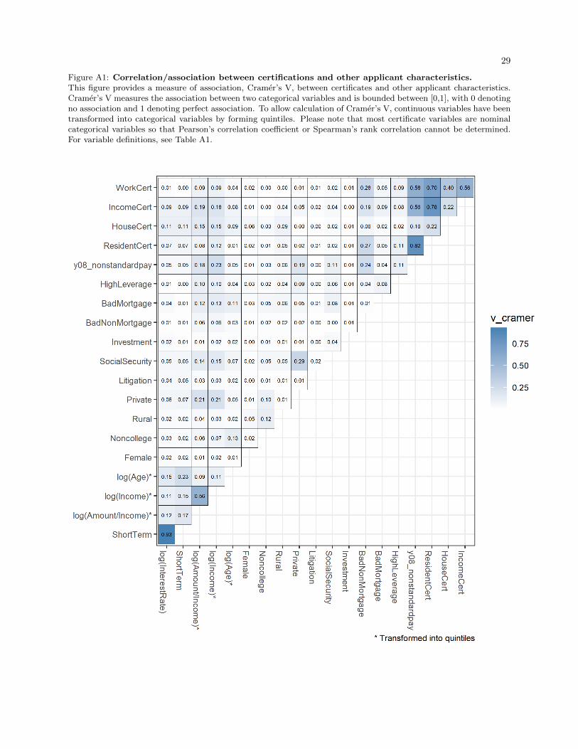
29
Figure A1: Correlation/association between certifications and other applicant characteristics.This figure provides a measure of association, Cramer’s V, between certificates and other applicant characteristics.Cramer’s V measures the association between two categorical variables and is bounded between [0,1], with 0 denotingno association and 1 denoting perfect association. To allow calculation of Cramer’s V, continuous variables have beentransformed into categorical variables by forming quintiles. Please note that most certificate variables are nominalcategorical variables so that Pearson’s correlation coefficient or Spearman’s rank correlation cannot be determined.For variable definitions, see Table A1.
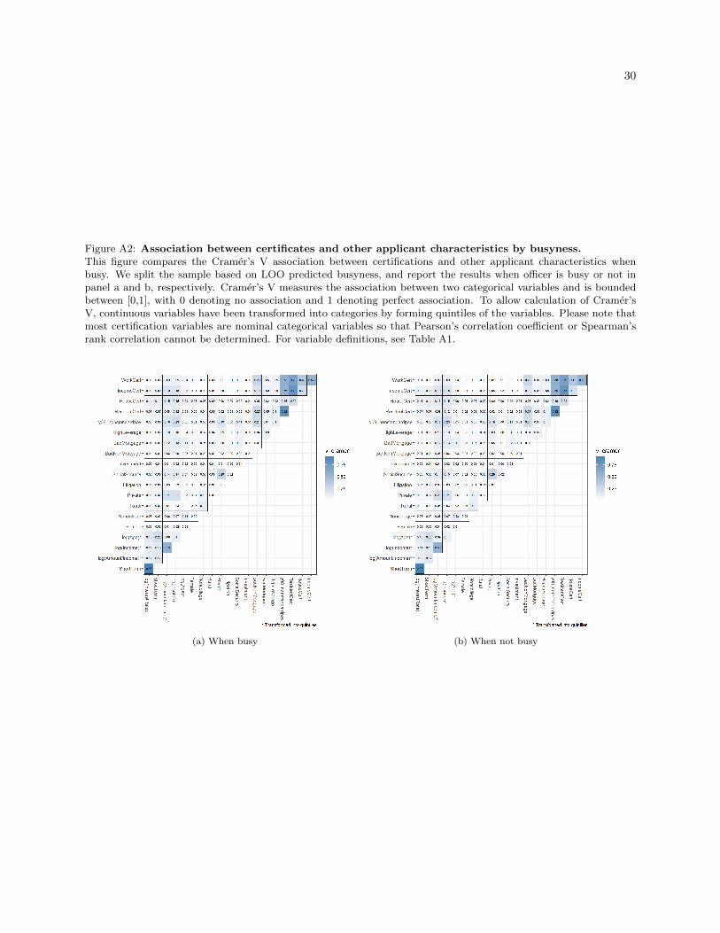
30
Figure A2: Association between certificates and other applicant characteristics by busyness.This figure compares the Cramer’s V association between certifications and other applicant characteristics whenbusy. We split the sample based on LOO predicted busyness, and report the results when officer is busy or not inpanel a and b, respectively. Cramer’s V measures the association between two categorical variables and is boundedbetween [0,1], with 0 denoting no association and 1 denoting perfect association. To allow calculation of Cramer’sV, continuous variables have been transformed into categories by forming quintiles of the variables. Please note thatmost certification variables are nominal categorical variables so that Pearson’s correlation coefficient or Spearman’srank correlation cannot be determined. For variable definitions, see Table A1.
(a) When busy (b) When not busy