Atom-Molecule Coherence in an Atomic Bose Gaswith a Feshbach Resonance.

Edmundo R. Sanchez Guajardo

November 6, 2004Utrecht, The Netherlands

Supervisor: Prof. Dr. Ir. H.T.C. Stoof and Drs. M.W.J. Romans

2

1 Foreword

This thesis presents the results of the research done between February and August 2004for the Masters Program in Theoretical Physics at the Utrecht University. The researchwas done under the supervision of Prof.Dr.Ir. Henk T.C. Stoof and Drs. Mathijs W.J.Romans. The original objective of finding the dispersion of the elementary excitations, andthe Green function in order to find the particle fluctuations had to be partially changed tounderstanding the system in order to explain unexpected instabilities that appeared duringthe analysis.

3

4

Contents

1 Foreword 3

2 Introduction 7

3 Background Knowledge 103.1 Single-Channel Scattering Theory . . . . . . . . . . . . . . . . . . . . . . . . 103.2 Multi-Channel Scattering Theory- Feschbach Resonance . . . . . . . . . . . . 163.3 Landau Theory of Phase Transitions . . . . . . . . . . . . . . . . . . . . . . 213.4 Bogoliubov Theory . . . . . . . . . . . . . . . . . . . . . . . . . . . . . . . . 22

4 Bogoliubov Theory for a Bose Gas with a Feshbach Resonance 24

5 Gross-Pitaesvkii equations and the resulting chemical potential µ withoutnonresonant interactions. 295.1 Positive detuning (δ > 0) . . . . . . . . . . . . . . . . . . . . . . . . . . . . . 33

5.1.1 Large positive detuning, δ >> g√nm,c . . . . . . . . . . . . . . . . . 33

5.1.2 At the Feshbach resonance, δ = 0 . . . . . . . . . . . . . . . . . . . . 335.2 Negative detuning (δ < 0) . . . . . . . . . . . . . . . . . . . . . . . . . . . . 34

5.2.1 At the Feshbach resonance, δ = 0 . . . . . . . . . . . . . . . . . . . . 345.2.2 At the quantum critical point δ = δcrit . . . . . . . . . . . . . . . . . 35

6 Condensate densities nm,c and na,c without nonresonant interactions 37

7 Dispersions hωa and hωm 397.1 Atomic dispersion hωa for positive detuning (δ > 0) . . . . . . . . . . . . . . 397.2 Molecular dispersion hωm for positive detuning (δ > 0) . . . . . . . . . . . . 417.3 Atomic dispersion hωa for negative detuning (δ < 0) . . . . . . . . . . . . . . 447.4 Molecular dispersion hωm for negative detuning (δ < 0) . . . . . . . . . . . . 44

8 Expansion of hωa and hωm 478.1 Expansion of atomic dispersion hωa,s for positive detuning. . . . . . . . . . . 488.2 Expansion of molecular dispersion hωm,s for positive detuning. . . . . . . . . 508.3 Expansion of atomic dispersion hωa,s for negative detuning. . . . . . . . . . . 518.4 Expansion of molecular dispersion hωm,s for negative detuning. . . . . . . . . 518.5 Comparison of atomic expansion with Bogoliubov theory . . . . . . . . . . . 52

9 Eigenvalues and Stability 569.1 Second-derivative test of the energy. . . . . . . . . . . . . . . . . . . . . . . . 569.2 Eigenvalues Considering the nonresonant Interactions Tij Individually . . . . 57

9.2.1 Atom-Atom interaction, Taa 6= 0 . . . . . . . . . . . . . . . . . . . . . 599.2.2 Molecule-Molecule interactions, Tmm 6= 0 . . . . . . . . . . . . . . . . 609.2.3 Atom-Molecule interaction, Tam 6= 0 . . . . . . . . . . . . . . . . . . . 619.2.4 Relation between Taa and Tam . . . . . . . . . . . . . . . . . . . . . . 62

5

9.3 Eigenvalues Considering the nonresonant Interactions Tij that IndividuallyStabilized the System . . . . . . . . . . . . . . . . . . . . . . . . . . . . . . . 629.3.1 Negative Detuning . . . . . . . . . . . . . . . . . . . . . . . . . . . . 639.3.2 Positive Detuning . . . . . . . . . . . . . . . . . . . . . . . . . . . . . 64

10 Gross-Pitaesvkii equations and the resulting chemical potential µ withnonresonant interactions. 6810.1 Positive detuning (δ > 0) . . . . . . . . . . . . . . . . . . . . . . . . . . . . . 6910.2 Negative detuning (δ < 0) . . . . . . . . . . . . . . . . . . . . . . . . . . . . 70

11 Condensate densities nm,c and na,c with nonresonant interactions Tij. 7211.1 Negative detuning (δ < 0) . . . . . . . . . . . . . . . . . . . . . . . . . . . . 7211.2 Positive detuning (δ > 0) . . . . . . . . . . . . . . . . . . . . . . . . . . . . . 73

12 Conclusions and Discussion 75

6

2 Introduction

The field of atomic quantum gases has recieved considerable attention in the last years.On the topic of an atomic gas of bosons and the corresponding Bose-Einstein condensation(BEC) in such a gas a comprehensive review is given by Anglin et al.[1]. A more theoreticalreview of the problem is given by Dalfovo et al.[2]. In order to reach the quantum-degenerateregime of the gas one has to cool it down to temperatures in which the atoms’ de Brogliewavelength λdB is larger than the average interatomic spacing. In the case of bosons, a cloudof atoms that are all in the single-particle ground state appears: this is the BEC. Hence,it would seem that creating a BEC is only a matter of cooling an atomic gas to sufficientlylow temperatures. This is not the case, however, because the more common transitions toa solid or a liquid would take place unless we also require the gas to have an extremelylow density. Only when the atomic gas is extremely diluted, three-body collisions and theformation of molecules are so improvable that they can be disregarded, leaving only binaryelastic collisions to be accounted for. The low density combined with the low temperaturerequired to reach quantum degeneracy places the temperature scale in the nanokelvin range.

Although the BEC is an ultra-low density and weakly-interacting system, its interactionscreate phase transitions, phonons, superfluidity and Josephson oscillations. Without interac-tions the BEC would be an ideal gas with properties similar to that of photons in an opticallaser. It is particularly appealing that the BEC of dilute atomic gases can be describedtheoretically from first principles.

On the theoretical side the task has been to develop an accurate description of this regime.The basic theory of weakly-interacting Bose gases requires that binary collisions are muchmore frequent than three-body collisions. This condition is equivalent to requiring that theaverage interatomic separation n−1/3 is much larger than the s-wave scattering length a, sincethe magnitude of the scattering length gives the typical range of the interatomic forces. Onthe other hand, the stability of the condensate requires repulsive interactions, for attractiveinteractions make the condensate collapse. The Gross-Pitaevskii-Bogoliubov theory describesthe various phenomena taking place at zero temperature quite well. The Gross-Pitaevskiiequation is a wave equation for the macroscopic matter-wave field of the condensate, and theBogoliubov theory describes the fluctuation around this coherent field (ground state). Eventhough the theory has proven successful in explaining experiments it has the shortcomingthat it violates the conservation of atoms. Nonetheless, the theory successfully describesthe interactions in the system. For instance, collisions between condensate atoms produce acoherent pressure that supports zero-sound density waves, whose wavelength is shorter thanthe mean free path. The theory also predicts superfluidity, which is defined as flow withoutdissipation. Since the theory is Galilean invariant, it does not depend on the reference frame.

The task on the experimental side has been to reach the extremely low temperaturerequired. The essential cooling techniques to reach sub-microkelvin temperatures combinetwo procedures: laser cooling and forced evaporative cooling. Laser cooling precools thegas, enabling its confinement in a magnetic trap. Forced evaporative cooling effectivelyreduces the depth of the trap, allowing the most energetic atoms to scape. Evaporativecooling requires the rate of elastic collisions to be higher than the rates of inelastic andbackground gas collisions. The way to understand this is that the elastic collisions establishthermal equilibrium, while inelastic and background collisions lead to trap loss and molecule

7

formation.The development of new techniques offers further flexibility in condensation. For instance,

’all optical’ cooling replaces the magnetic traps with an optical dipole trap formed by CO2

laser beams. Even though it permits lower densities, it is compensated by a more efficientevaporation: the atoms only escape at saddle points of the potential when reducing the inten-sity of the laser, instead of the all-round escape of magnetic traps. It allows the confinementof atoms with magnetic moments too small for magnetic trapping, and the condensationof atoms with high spin-flipping losses. However, magnetic traps have also been improved:their miniaturization results in tight confinement and a reduction in the required power.Another innovation to compensate for unfavorable collisions has been to add to the gas anatomic species that responds very effectively to evaporative cooling. This so-called sympa-thetic cooling is particularly important for fermions, because the Pauli exclusion principleinhibits collisions between fermions of the same species at low temperatures.

Especially interesting to our discussion is the possibility to directly modify the collisionproperties of the atoms. At the low temperatures of interest, the interaction energy ofa cloud of atoms is proportional to the density of particles and to the scattering length a,which depends on the quantum mechanical phase shift in an elastic collision. The control overthe atoms is achieved through smooth background fields. These may be external magnetic,optical or radio-frequency fields. At particular field strengths the energy of a (quasi)boundmolecular state may be shifted to zero, and at that point it couples resonantly to the free stateof the colliding atoms. This is the Feshbach resonance. In a time-dependent picture, the twoatoms are transferred to the (quasi)bound state, stay a finite time in this state, and finallyreturn to an unbound state. For repulsive interactions, the (quasi)bound state has an infinitelifetime, and is thus a real molecule. While for attractive interactions the (quasi)bound statehas a finite lifetime, which leads to difficulties in the theoretical formalism.

As described in [3], the effective scattering length a covers the full continuum of positiveand negative values above and below a Feshbach resonance. By setting a ≈ 0, one can createa condensate with basically non-interacting atoms, while by tuning a < 0 the attractiveinteractions make the system unstable and lead to its collapse. Nevertheless, the Feshbachresonant atom-molecule coupling can create a second condensate component of moleculesthat coexist with the atomic condensate. For a > 0 the repuslive interactions result in astable condensate with real molecules or a condensate of both atoms and molecules dependingon the temperature. Experimental results are shown in Fig. 1. At resonance one finds acondensate of gapless molecules coupled to a condensate of atoms. Far off resonance, the gascontains essentially a single atomic condensate with an effective binary collision scatteringlength on the a < 0 side and a purely molecular BEC in the case of a > 0. Interestingly, fora < 0 even far from resonance we would expect to find a molecular condensate coexistingwith the atomic one.

8

Figure 1: Experimental results by Inouye, et al.[3]. Theupper graph gives the depletion of the condensate due tostrong interactions, indicate the Feshbach resonance. Inthe lower graph the divergence and change of sign of thescattering length at the resonance is shown.

9

3 Background Knowledge

3.1 Single-Channel Scattering Theory

Here we give a relatively brief description of the single-channel scattering problem followingthe lines of [4] and [5]. Before describing single-channel scattering formally let us identify thefour possible scattering situations depending on the sign of the energy E and of a scatteringpotential V0 as summarized in table below:

E > 0 E < 0V0 > 0 Transmission(E > V0) Reflection/Tunneling(E < V0)V0 < 0 Scattering Boundstate

Hence, in a first effort to explain how a bound state depends on a tunable potential, letus look at a similar case in a single channel, as described in Fig. 2. The potential well V0

clearly corresponds to an attractive V0 < 0 potential. Meanwhile, the potential barrier V ′0

corresponds to a repulsive potential V ′0 > 0. Clearly, a particle incoming from the right with

energy 0 < E < V ′0 will form a (quasi)bound state only when it manages to tunnel through

the barrier. If the energy of the incoming particle lies below the resonant threshold at whichthe potential changes from repulsive to attractive, i.e., E < 0, then a real bound state maybe formed if the potential well is ”deep” enough.

Let us now start our discussion by considering the scattering of two particles with nointernal degrees of freedom and reduced mass m = m1m2/(m1 +m2). After transforming tothe center-of-mass of the particles, one finds that in the limit r → ∞ the scattering wavefunction for the relative motion is the linear superposition of an incoming plane wave and ascattered wave,

ψ(~r) = eikz + ψsc(~r), (1)

where the relative velocity in the incoming wave was chosen to be in the z direction. Theproces is discribed in Fig. 3. The scattered wave is actually an outgoing spherical wave, so

ψsc(~r) = f(θ)eikr

r, (2)

where spherically symmetric interactions between atoms were assumed in order to write thewave vector ~k of the scattering amplitude f(θ) in terms only of the scattering angle θ. Thus,the wave function in the limit r →∞ becomes

ψ(~r) = eikz + f(θ)eikr

r, (3)

with the corresponding energy of the state given by

E =h2k2

2m. (4)

10

V0

V(r)

rE

'V 0

Figure 2: If the energy of the particle is 0 < E < V ′0 it

is a quasibound state with finite life time. On the otherhand, if E < V0 there may be a bound state. The numberof bound states depends on the depth of the attractivepotential as can be seen in the inset, where the depth ofthe potential is parametrized by γ and each new boundstate is indicated by the divergence and change of sign ofthe scattering length a.

At very low energies (like the ones we are interested in) it is sufficient to consider s-wavescattering. In this limit, the scattering amplitude f(θ) approaches a constant that we denoteby −a, and we refer to a as the scattering length. Hence, in this low energy limit, k ≈ 0, thewave function becomes for r >> a

ψ(~r) = 1− a

r. (5)

The scattering length gives the intercept of the asymptotic wave function (5) on the raxis. In addition, the scattering length is connected to the phase shift, which in generaldetermines the scattering cross section. In order to establish the connection between thescattering length and the phase shift we change momentarily our discussion and start fromthe differential cross section

dσ

dΩ= |f(θ)|2, (6)

which is the cross section per unit solid angle. We know the differential surface element ofa sphere is given by dΩ = 2π sin θdθ. Thus, the differential cross section becomes

dσ = 2π sin θ|f(θ)|2dθ. (7)

The problem has been reduced to finding |f(θ)|. To do this we note that the sphericallysymmetric potential results in an axially symmetric solution of the Schrodinger equation

11

q k'

k

z

V(r)

Figure 3: Elastic scattering between an incoming particlemoving in the z direction with momentum ~k and an out-going particle with momentum ~k′ for a particular V (r).For elastic scattering, the magnitude of the momenta isthe same, and the direction is changed by the angle θ.

with respect to the incident particle. Therefore, the wave function of the relative motionψsc(~r) may be expanded in terms of Legendre polynomials Pl(cos θ) by a function of theform,

ψ(~r) =∞∑l=0

AlPl(cos θ)Rkl(~r)

r. (8)

The functionRkl(~r) is a radial wave function that satisfies the corresponding radial Schrodingerwave function

R′′kl(~r) +

2

rR′kl(~r) +

[k2 − l(l + 1)

r2− 2m

h2 V (r)

]Rkl(~r) = 0, (9)

where V (r) is the potential, and the derivatives are with respect to the radial coordinate r.Expression (9) is complicated, and it seems we have not gained much. Nonetheless, in thelimit r −→∞ the radial function is given in terms of the phase shift δl by the expression

Rkl(r) ≈1

krsin(kr − π

2l + δl). (10)

After substituting this expression for Rkl(~r) into Eq. (8), it can be compared with ψsc(~r) inEq. (4). After also expanding the incoming plain wave exp(ikz) one finds Al = il(2l+ 1)eiδl ,and more important for our purposes that

f(θ) =1

2ik

∞∑l=0

(2l + 1)(ei2δl − 1)Pl(cos θ). (11)

12

Notice how f(θ) only depends on the phase shift. This scattering amplitude is useful forfinding the total scattering cross section, which is the integral of the differential cross sectionover all solid angles, i.e.,

σ = 2π∫ 1

−1d(cos θ)|f(θ)|2. (12)

Bearing in mind that the Legendre polynomials are orthogonal when performing this integralusing (11), the total cross section in terms of the phase shift is found to be

σ =4π

k2

∞∑l=0

(2l + 1) sin2 δl. (13)

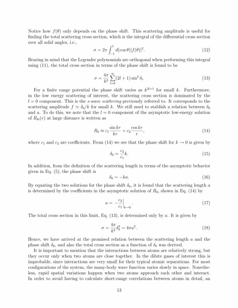
For a finite range potential the phase shift varies as k2l+1 for small k. Furthermore,in the low energy scattering of interest, the scattering cross section is dominated by thel = 0 component. This is the s-wave scattering previously referred to. It corresponds to thescattering amplitude f ' δ0/k for small k. We still need to stablish a relation between δ0and a. To do this, we note that the l = 0 component of the asymptotic low-energy solutionof Rkl(r) at large distance is written as

R0 ≈ c1sin kr

kr+ c2

cos kr

r, (14)

where c1 and c2 are coefficients. From (14) we see that the phase shift for k → 0 is given by

δ0 =c2c1k. (15)

In addition, from the definition of the scattering length in terms of the asymptotic behaviorgiven in Eq. (5), the phase shift is

δ0 = −ka. (16)

By equating the two solutions for the phase shift δ0, it is found that the scattering length ais determined by the coefficients in the asymptotic solution of R0, shown in Eq. (14) by

a = −c2c1

∣∣∣∣k→0

. (17)

The total cross section in this limit, Eq. (13), is determined only by a. It is given by

σ =4π

k2δ20 = 4πa2. (18)

Hence, we have arrived at the promised relation between the scattering length a and thephase shift δ0, and also the total cross section as a function of δ0 was derived.

It is important to mention that the interactions between atoms are relatively strong, butthey occur only when two atoms are close together. In the dilute gases of interest this isimprobable, since interactions are very small for their typical atomic separations. For mostconfigurations of the system, the many-body wave function varies slowly in space. Nonethe-less, rapid spatial variations happen when two atoms approach each other and interact.In order to avoid having to calculate short-range correlations between atoms in detail, an

13

effective interaction is introduced. It describes interactions among long-wavelength, low-frequency degrees of freedom of a system when the coupling of these degrees of freedom viainteractions with those of shorter wavelengths have to be taken into account. The shortwavelength degrees of freedom are said to have been ’integrated out’.

Effectively, the interactions appear in the Schrodinger equation as a potential V , and theylead to the two-body T-matrix and the Lippmann-Schwinger equation. The Schrodingerequation that needs to be solved is now

[H0 + V ] |ψ〉 = E |ψ〉 , (19)

with H0 = h2k2/2m the kinetic energy of the atoms, as before. That means that if there isno scattering, one finds H0| φ〉 = E| φ〉, where φ is the free-particle plain-wave function men-tioned before. If on the other hand there is scattering, we have [H0 + V ]|ψ >= E|ψ >. Sincewe are considering elastic scattering processes, the energy is conserved, which means thatthe energy E in both cases is the same. Moreover, we require that in the limit where there isno scattering, V → 0, the scattering wave function becomes the free particle wave function,| ψ〉 → | φ〉. The solution is then the linear superposition of both states. Furthermore, onecan see that the expression for |ψsc > satisfies

|ψsc〉 =1

E − H0

V |ψ〉 , (20)

which allows the solution |ψ >= |φ > +|ψsc > to be written as

|ψ(±) >=1

E − H0 ± iεV |ψ > +|φ > . (21)

The denominator has been made slightly imaginary in order to avoid any singularity, whichresults in |ψ >→ | ψ(±)

⟩. Equation (21) is known as the Lippman-Schwinger equation. It is

basis independent, which allows us to represent it into any representation. For instance, ifwe project it onto the momentum representation using the bra < k| one finds

< k|ψ(±) >=1

E − εk ± iε< k|V |ψ± > + < k|φ >, (22)

where εk = h2k2/2m is the relative kinetic energy of the particles as before. Notice that thisexpression is not yet useful because the function |ψ > is not known. This problem will alsoappear when discussing the Feshbach resonance in the next section.

In order to deal with this problem, we look at the Born approximation. In first order itallows the substitution of the general solution for the wave function | ψ〉 if the interactionsare not very strong. In higher order the stronger interaction considered do not allow forsuch a straightforward substitution. In that case, the scattering is taken into account whensubstituting the general solution by the plain wave by introducing the transition operator T .It is defined as

V | ψ(+)⟩

= T | φ〉 . (23)

If the Lippmann-Schwinger equation (21) is multiplied from the left by V , the definition ofthe T operator lets us write it as

T | φ〉 = V | φ〉+ V1

E − H0 + iεT | φ〉 . (24)

14

Hence, we have arrived at an equation that depends on the well known plain wave function| φ〉. We can read from it that the transition operator obeys

T (E) = V + V1

E − H0 + iεT . (25)

If Eq. (24) is now projected into the momentum representation with orthogonal states nor-malized by 〈k′|k〉 = (2π)3δ(k − k′), which we also know for φ, one finds that the scatteringamplitude is

f(k′, k) = − 1

4π

2m

h2

⟨k′|T |k

⟩, (26)

which means that the transition operator T defines the whole scattering process and letsus find the scattering amplitude f(k′, k) for an incoming particle of momentum k and anoutgoing particle of momentum k′ for our elastic process.

Hence, the problem has turned into finding the transition operator. The first three termsof (25) are clearly given by

T (E) = V + V G0(E)V + V G0(E)V G0(E)V + ..., (27)

where G0(E) = (E − H0 + iε)−1. Thus, we need to expand the scattering amplitude f inorder to be able to establish a relationship between the two. Noticing the linear increase ofthe number of times the potential V appears in Eq. (27), we expand f as a series in whichthe order indicates the number of times V appears in that term,

f(k′, k) =∞∑n=1

f (n)(k′, k). (28)

Now a clear correspondence between expressions (27) and (28) can be established. The firsttwo terms in the series are thus given by

f (1)(k′, k) =< k′|V |k >, (29)

f (2)(k′, k) =< k′|V G0(E)V |k > . (30)

If a pseudopotential is introduced

V (x− x′) =4πah2

µδ(x− x′), (31)

where µ = 2m is the real mass, we recover with the first term the previous scatteringamplitude f (1) = −a.

In addition, the transition operator T also allows us to look for the bound states of thepotential. To see this, we first realize after summing up all the terms in Eq. (27) that theresulting expression for the total T-matrix is

T (E) = V + V1

E − HV , (32)

where H = H0 + V is the full Hamiltonian with the energy states obeying H |ψ〉 = εα |ψ〉.The energy εα may be either of a bound state or a scattering state, namely, εα < 0 or

15

εα > 0, depending on the potential V . Clearly, a negative attractive potential could resultin a negative energy. Inserting a complete set of states ψα we can write Eq. (32) as

T (E) = V +∑κ

V|ψκ〉 〈ψκ|E − εκ

V +∫ dk

(2π)3V|ψk〉 〈ψk|E − 2εk

V , (33)

where the sum is over the bound state energy εκ, and the integral is over the continuousscattering states with energy εk. The factor of two in from of εk is due to the fact that thereduced mass obeys m = µ/2. Now we can clearly see that the bound states correspond tothe poles in the complex energy plane E = εκ. Also, the continuum of scattering states hasa branch cut, as can be seen in Fig. (4)

x xxxxx

Im(E)

Re(E)

Figure 4: The poles of the T-matrix on the negative en-ergy axes correspond to bound-states. On the positiveaxes the continuum of scattering states leads to a branchcut starting at the origin. [6]

3.2 Multi-Channel Scattering Theory- Feschbach Resonance

In this section we discuss the multi-channel scattering problem following the lines of Tim-mermans, et al.[7] We will arrive at an expression to describe the resonance that takes placein this scattering situation for two channels. The resonance in the binary atom interactionis caused by the hyperfine interaction. This interactions can flip both the electronic andnuclear spins of one of the colliding atoms. Namely, it changes the spin configuration ofthe colliding atom in the open (P)-channel into that of the close (M)-channel. While inthe M-channel, the colliding atoms form a (quasi)bound molecular state |φm〉. If the energyof this (quasi)bound state is equal to the continuum level of the P-channel, the previouslydescribed collision process is on resonance. Hence, an external magnetic field may be varied

16

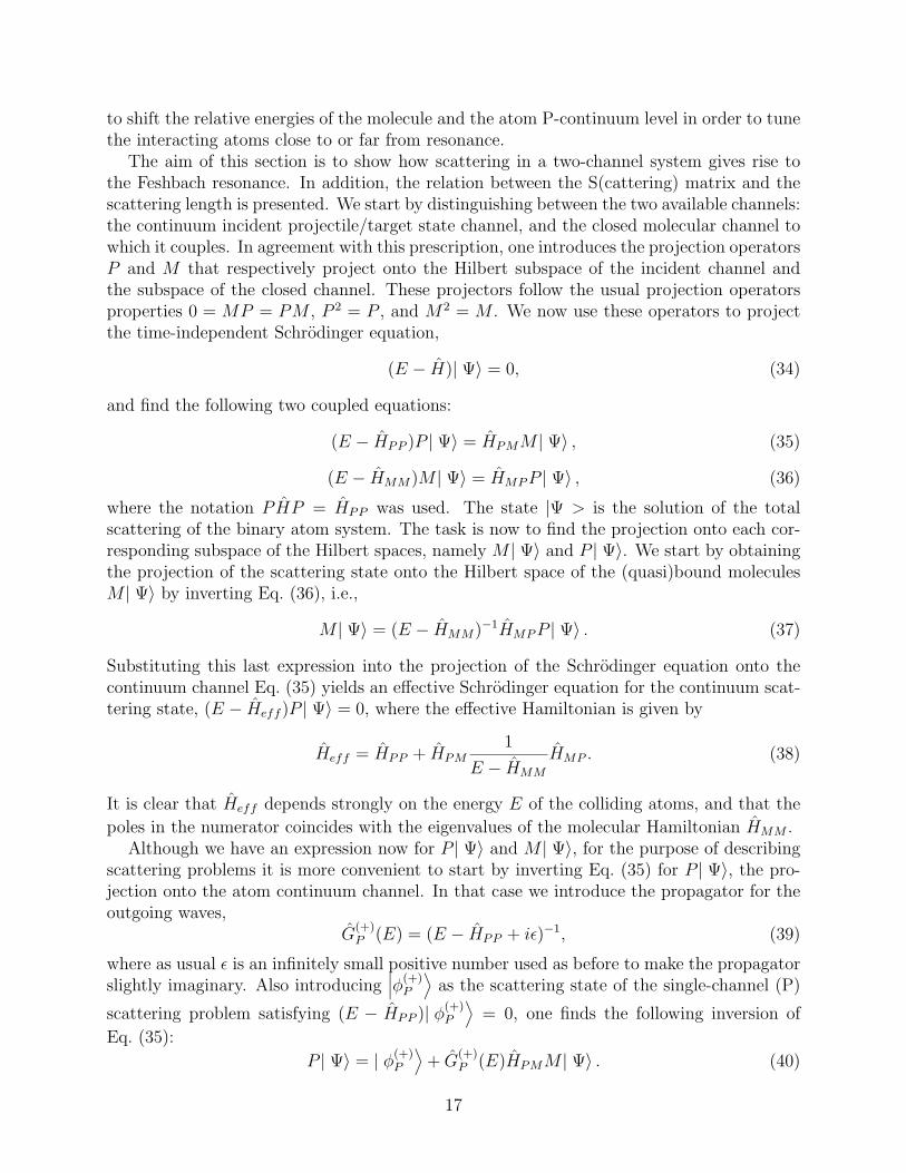
to shift the relative energies of the molecule and the atom P-continuum level in order to tunethe interacting atoms close to or far from resonance.

The aim of this section is to show how scattering in a two-channel system gives rise tothe Feshbach resonance. In addition, the relation between the S(cattering) matrix and thescattering length is presented. We start by distinguishing between the two available channels:the continuum incident projectile/target state channel, and the closed molecular channel towhich it couples. In agreement with this prescription, one introduces the projection operatorsP and M that respectively project onto the Hilbert subspace of the incident channel andthe subspace of the closed channel. These projectors follow the usual projection operatorsproperties 0 = MP = PM , P 2 = P , and M2 = M . We now use these operators to projectthe time-independent Schrodinger equation,

(E − H)| Ψ〉 = 0, (34)

and find the following two coupled equations:

(E − HPP )P | Ψ〉 = HPMM | Ψ〉 , (35)

(E − HMM)M | Ψ〉 = HMPP | Ψ〉 , (36)

where the notation PHP = HPP was used. The state |Ψ > is the solution of the totalscattering of the binary atom system. The task is now to find the projection onto each cor-responding subspace of the Hilbert spaces, namely M | Ψ〉 and P | Ψ〉. We start by obtainingthe projection of the scattering state onto the Hilbert space of the (quasi)bound moleculesM | Ψ〉 by inverting Eq. (36), i.e.,

M | Ψ〉 = (E − HMM)−1HMPP | Ψ〉 . (37)

Substituting this last expression into the projection of the Schrodinger equation onto thecontinuum channel Eq. (35) yields an effective Schrodinger equation for the continuum scat-tering state, (E − Heff )P | Ψ〉 = 0, where the effective Hamiltonian is given by

Heff = HPP + HPM1

E − HMM

HMP . (38)

It is clear that Heff depends strongly on the energy E of the colliding atoms, and that the

poles in the numerator coincides with the eigenvalues of the molecular Hamiltonian HMM .Although we have an expression now for P | Ψ〉 and M | Ψ〉, for the purpose of describing

scattering problems it is more convenient to start by inverting Eq. (35) for P | Ψ〉, the pro-jection onto the atom continuum channel. In that case we introduce the propagator for theoutgoing waves,

G(+)P (E) = (E − HPP + iε)−1, (39)

where as usual ε is an infinitely small positive number used as before to make the propagatorslightly imaginary. Also introducing

∣∣∣φ(+)P

⟩as the scattering state of the single-channel (P)

scattering problem satisfying (E − HPP )| φ(+)P

⟩= 0, one finds the following inversion of

Eq. (35):

P | Ψ〉 = | φ(+)P

⟩+ G

(+)P (E)HPMM | Ψ〉 . (40)

17

Furthermore, since∣∣∣φ(+)P

⟩is the scattering state within the P-channel we require that asymp-

totically it becomes a superposition of an incoming plane wave and an outgoing sphericalwave, as seen in Sec. 2.1, limr→∞φ

(+)P (~r) = exp(−i~k · ~r) − Sbg exp(ikr)/r. As previously

done, Eq. (40) for P |Ψ > is now inserted into the remaining coupled equation Eq. (36). Theresulting effective Schrodinger equation for M |Ψ > is

(E − HMM)M | Ψ〉 = HMP | φ(+)P

⟩+ HMPG

(+)P (E)HPMM | Ψ〉 . (41)

From this expression we find that M | Ψ〉 is given by

M | Ψ〉 =1

E − HMM − HMPG(+)P (E)HPM

HMP | φ(+)P

⟩, (42)

which we finally insert into Eq. (40) in order to find the resulting projection P | Ψ〉, i.e.,

P | Ψ〉 = | φ(+)P

⟩+G

(+)P (E)HPM

1

E − HMM − HMPG(+)P (E)HPM

HMP | φ(+)P

⟩. (43)

Finally we have two expressions for M | Ψ〉 and P | Ψ〉 in terms of the scattering state∣∣∣φ(+)P

⟩in the continuum. Notice how P | Ψ〉 is the continuum channel supersposition of incomingplane waves and outgoing spherical waves state, while M | Ψ〉 has no incoming wave andconsist only of an outgoing plain wave of the bound state. In order to find the S-matrixand consequently the scattering length we first further simplify Eq. (43) by noting that inthe low-energy Feshbach resonances we are interested in, each individual resonance is wellseparated in energy from one another. Hence, we may keep only a single diagonal matrixelement in evaluating the energy denominator. We may thus make the substitution

1

E − HMM − HMPG(+)P (E)HPM

→ |φm〉1

E − εm + iΓm/2〈φm| , (44)

where the energy εm and the width of the resonance Γm are given by:

εm = Re 〈φm| HMM − HMPG(+)P (εm)HPM |φm〉 , (45)

Γ

2= −Im 〈φm| HMPG

(+)P (εm)HPM |φm〉 . (46)

Notice that these equations are given in terms of the M channel states M |Ψ〉 = |φm〉.It is usefull in that case to remember that the ocupling between channels is weak, so wemay approximate |φm〉 as the eigenstate of the molecular potential, with the correspondingapproximate eigenvalue εm.

Let us now look in more detail at the width of the resonance. It is relevant to our discusionbecause it depends on the energy of the colliding atoms. Hence, in the ultra cold low-energysystems discussed here, we would expect it to be very narrow. Expanding G

(+)P (E) into the

continuum scattering states Eq. (4) gives

Γm2

= −Im

∑~k

|⟨φm|HMP |ψ~k

⟩|2

E − E~k + iε

= π∑~k

|⟨φm|HMP |ψ~k

⟩|2δ(E − E~k). (47)

18

Once again the matrix element < φm|HMP |ψ~k > is dominated by the s-wave component of|ψ~k >. Thus, it becomes

< φm|HMP |ψ~k >≈exp iδ0√

Vα, (48)

where α is a parameter related to the integral over the relative internuclear positions, andV is the normalization of the box assumed in the problem, i.e., it represents the confiningmacroscopic volume of the binary atom system. One finally finds that the width of theresonance is given by

Γ(E)

2=π

Vα2∑~k

δ(E − E~k), (49)

where it is clear that the only dependence is on the parameter α and the phase factor∑~k δ(E − E~k)/V related to the energy of the colliding atoms. In the continum limit the

sum over ~k becomes∫d3~k/(2π)3, since in a box with periodic boundary conditions in box-

normalization E~k = (π2h2n2)/2mL2, where (2π/L)~n is the wave number and L the length

of the box. Hence, after using that d3~k can be written as 2πkdk2 to express the integral interms of the energy E, we solve the integral and emphasize the energy dependence of theresulting width by introducing a reduced width γ, which obeys

Γm(E) = 2γk, (50)

with γ = α2m/(4πh2). The wave number k refers to the relative velocity of a pair ofatoms with kinetic energy E in the center-of-mass frame. Hence, as k → 0 we indeed findΓm(E) → 0, and γ remains constant.

We now turn our attention to the calculation of the desired S-matrix. We start by notingthat now the continuum scatter wave P |Ψ〉 is given by

P |Ψ〉 =∣∣∣φ(+)P

⟩+G

(+)P (E)HPM |φm〉

1

E − εm + iΓm/2〈φm| HMP

∣∣∣φ(+)P

⟩. (51)

It is once again evident that the denominator of Eq. (51) has poles depending on the molecu-

lar energy εm and the width of the resonance Γm. Furthermore, as already explained,∣∣∣φ(+)P

⟩is normalized so that its asymptotic r-dependence as r →∞ gives⟨

~r|φ(+)P

⟩= exp(−i~k · ~r)− exp(2iδbg) exp(ikr)/r, (52)

where δbg is the background s-wave phase shift. It has already been mentioned that in the lowenergy regime δbg = −kabg, where abg is the background scattering length. When evaluatingthe state given by Eq. (43) in the asymptotic region of coordinate space, 〈r|P |Ψ〉, it is also

useful to expand the s-wave component of the G(+)P -propagator as follows

[G

(+)P (E; r, r′)

]s

r→∞−→−(M

4πh2

)exp(iδ0)

exp(ikr)

ruN(r′), (53)

where r → ∞, and uN(r′) is the normalized regular solution of the Schrodinger equationwith the molecular potential [7]. One then finds the following asymptotic behavior for each

19

term in 〈r|P |Ψ〉:

limr→∞

〈r|G(+)P (E)HPM |φm〉 = −

(M

4πh2

)exp(iδ0)

exp(ikr)

r

∫d3r′uN(r′)HPMψm(r′)

= −(M

4πh2

)exp(iδ0)

exp(ikr)

rα. (54)

With the other matrix element < φm|HMP |φ(+)P >= −2ik exp(iδ0)α one finds the asymptotic

behavior

〈r|G(+)P (E)HPM |φm〉 〈φm| HMP

∣∣∣φ(+)P

⟩= i exp(2iδ0)

(M

2πh2

)α2k

exp(ikr)

r

= i exp(2iδ0)Γm(E)exp(ikr)

r. (55)

We finally find that the asymptotic r-dependence of the scattering state of Eq. (51) obeys

〈r|P |Ψ〉 ∼ exp(−i~k · ~r)−[1− iΓm

E − εm + iΓm(E)/2

]exp(2iδbg)

exp(ikr)

r. (56)

One then identifies from this expression that the S-matrix is

S =

[1− iΓm

E − εm + iΓm(E)/2

]exp(2ikabg), (57)

where δbg = −kabg was again used. In accordance to the scattering without loss channels,the S-matrix is unitary. In addition, the poles of the S-matrix are the bound states of thetwo-body problem. Moreover, it allows the introduction of the scattering length a. Thisleads to the scattering matrix S = exp(−2iak), where a = abg + ares, and

exp(−2iaresk) = 1− iΓmE(k)− εm + iΓm(E)/2

=E(k)− εm − iΓm/2

E(k)− εm + iΓm/2, (58)

with E(k) = (h2k2)/m. Finally, we find that the scattering length as a function of energyE(k) for k → 0 is given by

a(k) = abg +1

2ktan−1

[Γm [E(k)− εm]

(E(k)− εm)2 + Γ2m/4

]. (59)

In the ultra-low energy limit pertaining to condensate systems, E(k) vanishes for k → 0.In addition, in this limit the difference between the energy of the molecular state relative tothe continuum level of the P-channel gives rise to the detuning of the Feshbach resonance δ,E − εm → −δ. One then finds for the low energy limit

limE→0

a(E) = abg −γ

δ, (60)

20

where γ is the reduced width of the resonance. Experimentally, the strength of the magneticfield is the parameter available to control the resonance detuning. Moreover, when themagnetic field B takes its resonance value Bm, the energy of the (quasi)bound state εmmatches that of the incident atoms in the continuum. Therefore, the effective scatteringlength near resonance as a function of the external magnetic field strength takes the form

a = abg

[1− ∆B

B −Bm

]. (61)

Notice how away from resonance the difference B − Bm is large and makes a ≈ abg. Thus,we see that the resonance is superimposed on a smooth background scattering.

3.3 Landau Theory of Phase Transitions

This is a brief discussion of the Landau theory of phase transitions. Further reading may befound in [8]. Here we will discuss the Landau theory of phase transitions by first arrivingat the Landau free-energy and then discussing its two possible behaviors before reviewing inmore detail a second-order phase transition.

Let us start our discussion from the following functional integral over the vector orderparameter s(~x, t) for the partition function Z, that is given by

Z =∫d [s] e−S

eff [s]/h. (62)

The vector order parameter may have a non-zero average 〈s〉 related to a rotational invariantphysical property like magnetization or spin. For space and time independent fields, theaction Seff [s] is hβV fL(s), where fL(s) is the Landau free-energy density and V the totalvolume of the system. The Landau free-energy fL(s) has two possible behaviors dependingon whether it is a first-order or second-order phase transition. On the one hand, the first-order phase transition is characterized by a discontinuity in the order parameter at Tc andby the appearance of a second local minimum in the free energy fL(s) as the temperaturedecreases from T > Tc towards the critical temperature Tc. Exactly at Tc = T the localminimum is equal to that at s = 0. Finally, for T < Tc the local minimum has become theglobal minimum and 〈s〉 6= 0. On the other hand, in a second-order phase transition theorder parameter has no discontinuity as we cross Tc and the Landau free-energy fL(s) alwayshas one global minimum that changes to a non-zero value s 6= 0 for temperatures below Tc.Noticing that near Tc the order parameter 〈s〉 is very small in the case of a second-orderphase transition, we expand up to fourth order in s. We obtain

fL(s) = α(T )|s|2 +β

2|s|4, (63)

where there is no cubic term because the free energy must be symmetric under s → −s.Also important to note is that β > 0 and α(T ) = α0(T/Tc − 1). Thus, the change of signof α(T ) as we cross the critical temperature Tc effectively changes 〈s〉 = 0 for T > Tc to anonzero value for T < Tc given by

〈s〉 =

√α0

β

(1− T

Tc

). (64)

21

3.4 Bogoliubov Theory

In this subsection the dispersion relation of the collective excitations for a Bose-Einsteincondensate and the total density of the gas are derived [8]. At the same time, the Bogoli-ubov theory will be presented and the Gross-Pitaeski equation introduced. Let us start ourdiscussion from the following action S [φ∗, φ] for a gas of spin-less bosons, that is given by

S [φ∗, φ] =∫ hβ

0dτ∫d~xφ∗(~x, τ)

h∂

∂τ− h2∇2

2m+ V ex(~x)− µ

φ(~x, τ) (65)

+1

2

∫ hβ

0dτ∫d~xV0φ

∗(~x, τ)φ∗(~x, τ)φ(~x, τ)φ(~x, τ),

where φ∗(~x, τ) and φ(~x, τ) are real fields, and m is the atomic mass. This system showsthe phase transition to a Bose-Einstein condensate (BEC) that can be studied through theassociated order parameter < φ(~x, τ) >. This comes about because for time-independentfields φ(~x, τ) the action in Eq. (51) has the form of the Landau free energy. Furthermore, thecritical temperature must satisfy that the chemical potential µ(Tc) is equal to the groundstateenergy ε0, not only because this gives a vanishing contribution to the quadratic part of thefree energy, but also because it must follow the corresponding Bose statistics in the idealcase, namely,

N0 =1

eβ(ε0−µ) − 1. (66)

Clearly the number of particles in the ideal Bose gas one-particle ground state N0 divergeswhen µ = ε0.

In order to determine the corrections to the ideal gas case, we explicitly make the substi-tution φ(~x, τ) → φ(~x, τ) = φ0(~x) + φ′(~x, τ) into the action. Therefore, we intend to see theeffect of the fluctuations φ′(~x, τ) on the ground state or condensate φ0(~x). After performingthe substitution the action becomes

S [φ′∗, φ′] = hβFL [φ∗0, φ0] + S0 [φ′∗, φ′] + Sint [φ′∗, φ′] , (67)

where FL is the Landau free-energy, S0 contains the linear and quadratic terms in the fluc-tuating fields after the substitution, and Sint contains cubic and higher-order contributionsin the fluctuations. Thus far we have only expanded around the minimum. We now startusing the Bogoliubov approximation, in which we neglect Sint. Hence, we are left with S0.To make sure that 〈φ(~x, τ)〉 = φ0(~x) and 〈φ′(~x, τ)〉 = 0, we demand that the linear terms inthe fluctuations φ′ and φ′∗ drop out of S0. This gives the equation(

− h2∇2

2m+ V ex(~x) + V0(φ0(~x))

2

)φ0(~x) = µφ0(~x). (68)

This is the Gross-Pitaevskii equation for trapped atomic gases. It enables us on the onehand to determine the macroscopic condensate wave function φ0(~x), and on the other handto determine the chemical potential that places the system in the ground state. The totaldensity of the gas after substituting the expansion of the fields now obeys

n(x) =⟨φ(~x, τ)φ∗(~x, τ+)

⟩= (φ0(~x))

2 +⟨φ′(~x, τ)φ′∗(~x, τ+)

⟩. (69)

22

Let us emphasize and recapitulate that thus far we have determined an expression for themacroscopic ground-state wave function and the ground-state chemical potential throughthe Gross-Pitaevskii equation. We have derived an expression for the total density of the gasin Eq. (69) that includes the density of particles fluctuations, which follows from the actionSB in the Bogoliubov approximation that is quadratic in the fluctuations of the fields, i.e.,

SB [φ′∗, φ′] = − h2

∫ hβ

0dτ∫d~x [φ′∗(~x, τ), φ′(~x, τ)] ·G−1 ·

[φ′(~x, τ)φ′∗(~x, τ)

]. (70)

The problem is now to find the determinant of G−1 in order to find the dispersion of theelementary excitations and also to find its inverse G in order to find the required two pointfunction 〈φ′(~x, τ)φ′∗(~x, τ+)〉 to find the total density, since we have

−G(~x, τ ; ~x′, τ ′) =

⟨[φ′(~x, τ)φ′∗(~x, τ)

]· [φ′∗(~x, τ), φ′(~x, τ)]

⟩. (71)

To solve these two problems we start by realizing that

G−1(~x, τ ; ~x′, τ ′) = (72)

− 1

h

[G−1

0 (~x, τ ; ~x′, τ ′) + 2V0(φ0(~x))2 V0(φ0(~x))

2

V0(φ0(~x))2 G−1

0 (~x, τ ; ~x′, τ ′) + 2V0(φ0(~x))2

],

where

−hG−10 (~x, τ ; ~x′, τ ′) =

h∂

∂τ− h2∇2

2m+ V ex(~x)− µ

δ(~x− ~x′)δ(τ − τ ′). (73)

After substituting the chemical potential found from the Gross-Pitaeskii equation and Fouriertransforming into momentum space, one finds in the homogeneous case

G−1(k, iω) =

[−ihωn + εk + V0φ

20 V0φ

20

V0φ20 ihωn + εk + V0φ

20

]. (74)

Finding det[G−1] = 0 gives the poles of G(k, ω). Equivalently,

hω = hωk =√ε2k + 2V0(φ0)2εk =

√ε2k + 2V0n0εk. (75)

This is the Bogoliubov dispersion of the collective excitations. Interestingly, it may be written

as hωk =√εk(εk + 2V0n0), where it is clearly seen that hωk = 0 for εk = 0 and possibly for

εk = −2V0n0. Clearly, the second case does not happen if the potential is repulsive, V0 > 0.We still need to calculate the total density of the gas, i.e.,

n = φ20 −G11(x, τ ;x

′, τ ′) = n0 + n′. (76)

Therefore, we just need to find the matrix element G11(~x, τ ; ~x, τ+). We now proceed to

applying the theory reviewed in this section to our problem.

23

4 Bogoliubov Theory for a Bose Gas with a Feshbach

Resonance

We now want to apply the Bogoliubov theory, previously discussed, to analyze a Bose gasnear a Feshbach resonance (FR) explained in section 2.2. The resonance takes place at δ = 0.Furthermore, the Feshbach resonance is the mechanism to make a molecular Bose-Einsteincondensate. The molecular condensate phase can be reached in two ways as seen in thephase diagram Fig. 5: either the molecules are formed in the normal phase and then cooledbelow Tc into a molecular condensate phase, or the molecular condensate is formed withinan atomic condensate. We want to find again the total density of the gas and the dispersionrelation of the elementary excitations for the phase with an atomic condensate present, i.e.,〈Ψa〉 6= 0, which also has a molecular condensate 〈Ψm〉 6= 0. Furthermore, we limit ourselvesto the zero temperature case. Namely, for the detuning δ > δcrit, where δcrit is a quantumcritical point. For values of the detuning below δcrit the system consists solely of a molecularcondensate whenever the temperature is below its critical value, T < Tc, and it has beenstudied previously [6]. The system is described by the Hamiltonian [9] given by

0.3

0.4

0.5

-0.0005 0

0

0.2

0.4

0.6

0.8

1

1.2

-0.004 -0.003 -0.002 -0.001 0 0.001 0.002 0.003

T /

T0

δ / η2

MC AC+MC

Figure 5: Phase diagram of a Bose gas near a Feshbachresonance [9]. MC is the molecular condensate phase, andMC+AC is the atomic and molecular condensate phase.

H = H0 +Hint, (77)

where

H0 =∫d~xψ†m(~x)

[− h

2∇2

4m+ εm − 2µ

]ψm(~x) (78)

+∫d~xψ†a(~x)

[− h

2∇2

2m− µ

]ψa(~x)

24

−∫d~x√Zg

[ψ†m(~x)ψa(~x)ψa(~x) + ψm(~x)ψ†a(~x)ψ

†a(~x)

],

Hint =∫d~xTmm

2ψ†m(~x)ψ†m(~x)ψm(~x)ψm(~x) (79)

+∫d~xTaa2ψ†a(~x)ψ

†a(~x)ψa(~x)ψa(~x)

+∫d~xTamψ

†m(~x)ψ†a(~x)ψm(~x)ψa(~x).

The field operators ψ†m(x) and ψm(x) correspondingly create and annihilates a molecule atposition x, and ψ†a(x) and ψa(x) similarly create and annihilate an atom at position x. TheHamiltonian Hint contains the nonresonant two-body transition matrices for the scattering ofan atom with a dressed molecule Tam, two molecules Tmm, and two atoms Taa = 4πabgh

2/mwith abg the background scattering length and m the mass of the particles involved in theprocess. [9] In our discussion the nonresonant Tij have units of energy over density. TheHamiltonian H0 contains de resonant interaction. In it we find the molecular wave functionrenormalization factor Z, which implies that the wave function of the molecules is stronglyaffected by the interaction with the atomic continuum in the incoming channel and containsonly with an amplitude

√Z the molecular wave function χm(x) of the bound state in the

close channel, i.e.,

|Ψm〉 =√Z(δ) |χm〉+

√1− Z(δ) |Ψa〉 . (80)

The normalization Z was found [9] to be Z = 1 for positive detuning, and for nega-

tive detuning Z(δ) =(√

|2δ +√

1− 4δ − 1|)/(√

|2δ +√

1− 4δ − 1|+ 2−12

). Hence, the

molecular state |Ψm〉 is the superposition of the bare molecular wave function |χm〉 and theatom continuum |Ψa〉. Consequently, the field ψm is referred to as the dressed molecularfield. The constant g is the atom-molecule coupling, which has already been renormalizedin previous studies by doing a ladder summation that disregards many-body effects andconsiders the small momentum and energies discussed here [10]. Introducing c, which isthe scaled squareroot of the density, we may write g = (cη2)/

√nT . The parameter η2 has

units of energy, and nT is the total condensate density of the system. For our discusion, wetake c = 1.51214 × 10−5, which is a common value for experiments using 85Rb. Hence, thecoupling constant g is positive, real and independent of the detuning.

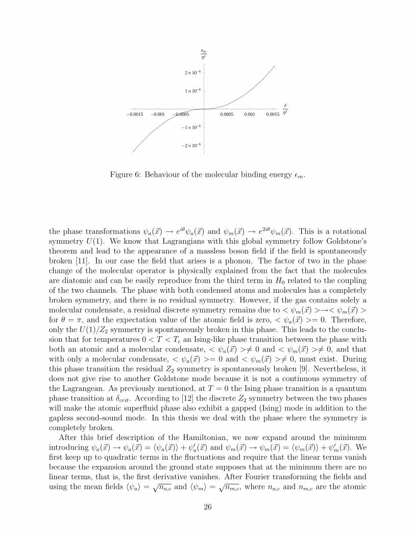
The bound-state energy of the molecules, shown in Fig. 6, is represented by εm and µ isthe chemical potential of the system. The bound state energy was found [9] to be

εm(δ) =εm(δ′)

η2= (δ′ − 1/2 +

√1/4− δ′ + 4δ′2)/3 (81)

for positive detuning, and

εm(δ) =εm(δ′)

η2= (2δ′ +

√1− 4δ′ − 1)/2 (82)

for negative detuning. The detuning δ′ is the scaled detuning δ/η2. In what follows we dropthe prime and unless otherwise specified we refer to δ′ as simply the detuning.

The symmetries of the gas described by this Hamiltonian are extremely relevant in under-standing the different phases of the system. The normal phase of the gas is invariant under

25

0.0015 0.001 0.0005 0.0005 0.001 0.0015

∆Η2

2106

1106

1106

2106

ΕmΗ2

Figure 6: Behaviour of the molecular binding energy εm.

the phase transformations ψa(~x) → eiθψa(~x) and ψm(~x) → e2iθψm(~x). This is a rotationalsymmetry U(1). We know that Lagrangians with this global symmetry follow Goldstone’stheorem and lead to the appearance of a massless boson field if the field is spontaneouslybroken [11]. In our case the field that arises is a phonon. The factor of two in the phasechange of the molecular operator is physically explained from the fact that the moleculesare diatomic and can be easily reproduce from the third term in H0 related to the couplingof the two channels. The phase with both condensed atoms and molecules has a completelybroken symmetry, and there is no residual symmetry. However, if the gas contains solely amolecular condensate, a residual discrete symmetry remains due to < ψm(~x) >→< ψm(~x) >for θ = π, and the expectation value of the atomic field is zero, < ψa(~x) >= 0. Therefore,only the U(1)/Z2 symmetry is spontaneously broken in this phase. This leads to the conclu-sion that for temperatures 0 < T < Tc an Ising-like phase transition between the phase withboth an atomic and a molecular condensate, < ψa(~x) >6= 0 and < ψm(~x) >6= 0, and thatwith only a molecular condensate, < ψa(~x) >= 0 and < ψm(~x) >6= 0, must exist. Duringthis phase transition the residual Z2 symmetry is spontaneously broken [9]. Nevertheless, itdoes not give rise to another Goldstone mode because it is not a continuous symmetry ofthe Lagrangean. As previously mentioned, at T = 0 the Ising phase transition is a quantumphase transition at δcrit. According to [12] the discrete Z2 symmetry between the two phaseswill make the atomic superfluid phase also exhibit a gapped (Ising) mode in addition to thegapless second-sound mode. In this thesis we deal with the phase where the symmetry iscompletely broken.

After this brief description of the Hamiltonian, we now expand around the minimumintroducing ψa(~x) → ψa(~x) = 〈ψa(~x)〉+ ψ′a(~x) and ψm(~x) → ψm(~x) = 〈ψm(~x)〉+ ψ′m(~x). Wefirst keep up to quadratic terms in the fluctuations and require that the linear terms vanishbecause the expansion around the ground state supposes that at the minimum there are nolinear terms, that is, the first derivative vanishes. After Fourier transforming the fields andusing the mean fields 〈ψa〉 =

√na,c and 〈ψm〉 =

√nm,c, where na,c and nm,c are the atomic

26

and molecular condensate density correspondingly, the Hamiltonian becomes

H −→ H ′ = 〈H〉+H ′0 +H ′

nr, (83)

In this expresion 〈H〉 is the Hamiltonian of the ground state containing only mean fields,the term

H ′0 =

∑k

[ψ′†m(k)

(εk2

+ εm − 2µ)ψ′m(k) (84)

+ ψ′†a (k) (εk + µ)ψ′a(k)

− 2g√Zna,c

(ψ′†m(k)ψ′a(k) + h.c.

)− g

√Znm,c (ψ

′a(k)ψ

′a(−k) + h.c.)

]contains the resonant interaction, and

H ′nr =

∑k

[Taa2na,c

(ψ′†a (k)ψ′†a (−k) + h.c.

)(85)

+ 2Taana,cψ′†a (k)ψ′a(k)

+ Tmmnm,c(ψ′†m(k)ψ′†m(−k) + h.c.

)+ 2Tmmnm,cψ

′†m(k)ψ′m(k)

+ Tam√nm,cna,c

(ψ′†a (k)ψ′†m(−k) + h.c.

)+ Tamna,cψ

′†m(k)ψ′m(k)

+ Tamnm,cψ′†a (k)ψ′a(k)

+ Tam√nm,cna,c

(ψ′†a (k)ψ′m(k) + h.c.

)]contains the nonresonant interactions. Therefore, if one also considers the derivatives withrespect to time in order to determine the action,

SB[ψ′†m, ψ′m, ψ

′†a , ψ

′a] =

∫ hτ

0dτ∫dk

[ψ′†mh

∂

∂τψ′m + ψ′†a h

∂

∂τψ′a +H ′

], (86)

one finds that the action can be written as SB =∫dk (Ψ| − hG−1 |Ψ), where

−hG−1(k, ω) = −hG−10 (k, ω) + hΣnr(k, ω), (87)

−hG−10 (k, ω) =

1

2

−hω + εk

2+ εm − 2µ 0 −2g

√Zna,c 0

0 hω + εk2

+ εm − 2µ 0 −2g√Zna,c

−2g√Zna,c 0 −hω + εk − µ −2g

√Znm,c

0 −2g√Zna,c −2g

√Znm,c hω + εk − µ

,(88)

hΣnr(k, ω) = (89)

1

2

2Tmmnm,c + Tamna,c Tmmnm,c Tam

√na,cnm,c Tam

√na,cnm,c

Tmmnm,c 2Tmmnm,c + Tamna,c Tam√na,cnm,c Tam

√na,cnm,c

Tam√na,cnm,c Tam

√na,cnm,c 2Taana,c + Tamnm,c Taana,c

Tam√na,cnm,c Tam

√na,cnm,c Taana,c 2Taana,c + Tamnm,c

,

27

and the fields

(Ψ| =[ψ′†m(hω, k), ψ′m(−hω,−k), ψ′†a (hω, k), ψ′a(−hω,−k)

]. (90)

Clearly, G−10 contains the resonant term of the inverse Green’s function, and Σnr contains

the nonresonant terms. Therefore, the corresponding partition function is

Z =∫d[ψ†m]d[ψm]d[ψ†a]d[ψa]e

− 1hSB[ψ†

m,ψm,ψ†a,ψa]. (91)

Thus far, we have obtained an effective action SB in momentum space that is quadraticin the fluctuations of the fields around the ground state. The action was written such thatthe inverse Green’s function was clearly identified. We now proceed to finding the chemicalpotential in order to fix the energy reference of the system with respect to the ground state,ε0 = µ(Tc).

28

5 Gross-Pitaesvkii equations and the resulting chemi-

cal potential µ without nonresonant interactions.

In this section the chemical potential of the system is derived through the Gross-Pitaevskiiequation and subsequently discussed for different values of the detuning. This equation isa Schrodinger equation for the macroscopic condensate wave function. Consequently, thechemical potential obtained from it allows us to fix our energy reference value with respectto the ground-state energy ε0. Therefore, we will ensure that the lowest energy of the systemleads indeed to a gapless dispersion for the atoms and a gapped one for the molecules. Notehowever, that in this section only the resonant interactions are being consider, which differfrom those of the free Bogoliubov theory because they are two-body processes.

Let us start our discussion by mentioning that in chemical equilibrium the whole systemhas the same chemical potential µ, which means that there is no net exchange of particles.We may now introduce the effective chemical potentials µa = µ and −µm = εm − 2µ, forthe atoms and the molecules correspondingly [13]. We do this particularly for µm becausethe expression will appear repeatedly, and we try to stablish its physical meaning. Themotivation for the minus sign in the molecular case is that in the absence of the energy shiftεm, we would like to recover µm = 2µ.

The normal phase of the ideal gas mixture is stable for µa < 0 and µm < 0. It is the tran-sitions between the normal phase and the condensed phases that require the correspondingeffective chemical potential to be zero. Clearly this requires on the one hand that µm = 0for δ < 0 for the transition from normal phase to molecular condensate phase to occur,while on the other hand that the µa = 0 for δ > 0 for the transition from normal phaseto atomic condensate to take place [12]. Hence, we want to explain how it behaves in ourzero-temperature approximation.

In what follows, when referring to the chemical potential we mean the chemical potentialµ of the system. Hence, in order to find the chemical potential µ we require that the linearterms in the fluctuations of the fields vanish from the action SB, i.e., they vanish from theHamiltonian,

∑i

δH

δψ′†m

∣∣∣∣∣ψ′†

i ,ψ′i=0

= 0 (92)

∑i

δH

δψ′†a

∣∣∣∣∣ψ′†

i ,ψ′i=0

= 0. (93)

Since in this section the nonresonant interactions are not yet being considered, only theresonant H ′

0 contributes to µ. The resulting Gross-Pitaevskii equations are

0 =δH ′

0

δψ′†m=

∫dx

[− h

2∇2

4m+ εm − 2µ

]〈ψm〉 (94)

−∫dx√Zg 〈ψa〉 〈ψa〉 ,

0 =δH ′

0

δψ′†a=

∫dx

[− h

2∇2

2m− µ

]〈ψa〉 (95)

29

− 2∫dx√Zg 〈ψm〉

⟨ψ†a⟩.

Furthermore, in the case of a homogeneous gas, the ground-state wave functions (con-densates) do not depend on the position. Hence, after substituting the mean-field values〈ψm〉 =

√nm,c and 〈ψa〉 =

√na,c these equations become

√Zgna,c = [εm − 2µ]

√nm,c, (96)

and2√Zg√nm,c = −µ. (97)

One finds the following two equivalent equations for the chemical potential µ,

µ =1

2

[εm − gna,c

√Z

nm,c

], (98)

µ = −2g√Znm,c. (99)

Nonetheless, we would like to have the chemical potentials written in a way that resemblesthe Bogoliubov one, µB = V0n0, in order to compare them. Since we have two expressionsfor the chemical potential, we use equation (99) to rewrite nm,c in equation (98). One finds

µ =2Zg2

2µ− εmna,c, (100)

µ = −2g√Znm,c. (101)

We now introduce an effective scattering interaction Teff given by the equation

Teff =−2Zg2

εm − 2µ. (102)

Thus, one finds the following two equivalent expressions, shown in Fig. 9 and in Fig. 10,for the chemical potential

µ = Teffna,c, (103)

µ = −2g√Znm,c. (104)

If we introduce the scaled dimensionless quantities µ, nm,c, na,c, and Teff we finally find that

Teff =nTTeffη2

=−2Zc2

εm − 2µ, (105)

µ =µ

η2= Teff na,c, (106)

µ =µ

η2= −2c

√Znm,c, (107)

30

0.0015 0.00125 0.001 0.00075 0.0005 0.00025

∆Η2

0.00014

0.00012

0.0001

0.00008

0.00006

0.00004

0.00002

nT TeffΗ2

Figure 7: Teff (δ < 0) diverges for the quantum criticalpoint δ = δcrit and vanishes at the Feshbach resonanceδ = 0.

It is interesting to note in Fig. 7 for Teff that it diverges for the quantum critical pointδ = δcrit. The divergence is due to 2µ = εm. On the other hand, Teff at δ ↑ 0 does notdiverge even though 2µ = 0 and εm = 0. That the molecular binding energy vanishes due tothe divergent scattering lenght is most easily seen from the expression

εm = − h2

m[a(B)]2, (108)

that describes the behaviour of εm close to resonance . Thus, the reason why Teff does notdiverge is because Z(0) = 0 on the negative detuning side, which makes it vanish.

Interestingly, as seen in Fig. 8 for the positive detuning region (δ > 0) the effectivescattering interaction Teff does not vanish at δ = 0. Although one finds the energy εm = 0,the chemical potential is not zero. This is due to the constant value of Z(δ) for positivedetuning, Z(δ) = 1, which on the negative detuning side has the value Z(0) = 0. Hence, thechemical potential behaves differently at δ = 0 through its dependence on Z(δ) dependingon whether it is approached from an increasing negative detuning or a decreasing positivedetuning. Therefore, the renormalization Z(δ) introduces into the theory a certain errorclose to resonance due to its approximative nature when considering the finite lifetime of themolecular quasibound state and its unlocalized density of states. Consequently, throughoutthe calculations one recurrently meets discontinuities on the values of the different variablesat δ = 0 depending on whether one considers δ > 0 or δ < 0. Be that as it may, since wewould expect to find a condensate of both atoms and molecules at δ ≈ 0 the normalizationZ should probably also become nonzero on the negative detuning side at resonance, due tomany-body effects.

The two expressions for µ can now be compared to the usual Gross-Pitaeskii equations ofthe Bogoliubov theory for an atomic BEC. That µ < 0 can be understood as follows: on the

one hand, for µ = −g√Z(δ)nm,c(δ) one has Z(δ) > 0 and nm,c(δ) > 0. Hence, the overall

minus sign is accountable for the negative value of µ as given in Eq. (104). Moreover, since

31

0.005 0.01 0.015 0.02 0.025 0.03

∆Η2

8106

6106

4106

2106

nT TeffΗ2

Figure 8: Teff (δ > 0) does not diverge at δ = 0 becauseµ has a non-zero value through its dependence on Z(δ).

the chemical potential of the system is the same as the effective atomic chemical potential,µ = µa, the atomic condensate also has an effective negative chemical potential. On theother hand, the expression µ = Teff (δ)na,c(δ) is negative because Z(δ) > 0, na,c(δ) > 0,and Teff (δ) < 0. Furthermore, one sees that Teff < 0 always because εm > 2µ through allthe values of the detuning considered here. This actually means that the effective chemicalpotential of the molecules −µm = εm − 2µ is always negative. Hence, the T-matrix Teff isnegative, which compared with the usual Bogoliubov µ = V0n0 would mean V0 < 0. Thismeans attractive interactions and thus an unstable condensate. Clearly, the Bogoliubovdispersion would be zero twice in that case. Nevertheless, since so far we are not consideringnonresonant scattering, but only the resonant coupling between channels, we realize thatthe chemical potentials given by Eq. (103) and Eq. (104) are not the same as that of theBogoliubov theory. They are caused by the coupling between channels, that is modified bythe external magnetic field applied to the system.

The emphasis on the negative sign of µ and its comparison with the Bogoliubov case is tostress that thus far we are dealing with the resonant part of the action and to make evidentthe importance of the nonresonant interactions for the realization of a BEC. Interestingly,G−1

0 has µ < 0 for every value of the detuning, like the ideal Bose gas.1 Clearly for theideal case µ < 0, but for the interacting case where we have both thermal and quantumfluctuations in the number of particles the chemical potential may become positive, as in theBogoliubov case.

1The density of states f = (e(εn−µ)/τ −1)−1 of an ideal Bose gas in the low temperatures and momentumwe are interested in becomes the number of particles f ≈ N = −τ/µ after expanding the exponential to firstorder. Clearly µ = −τ/N < 0. Moreover, the chemical potential should always be lower in energy than theground state energy in order to have all the occupancy of the energy orbitals positive.[14]

32

5.1 Positive detuning (δ > 0)

There are two limiting cases for positive detuning: one is at the Feshbach resonance δ = 0,and the other is when the two channels are effectively decoupled at large positive detuning.From the effective molecular chemical potential we see that at this second point εm >> 2µ,thus we stablish that large positive detuning means δ >> g

√nm,c.

5.1.1 Large positive detuning, δ >> g√nm,c

Starting with the later situation we see that the chemical potentials increase to zero, which isexactly what we would expect because the number of condensed molecules decreases as thedetuning increases. Thus, we are left with a condensate of atoms, which we would expect tohave a chemical potential that behaves like the well known µ = −τ/N for an ideal boson gasin the low energy limit, where N is the total number of particle in the system, and τ = kBT isthe temperature T in energy units with kB the Boltzman constant. This can be understoodbecause for zero temperature and the resonant interaction, then indeed µ → 0 as nm,c → 0when τ → 0, because for large positive detuning the two channels effectively decouple.

Looking at both expressions for µ separately, one sees that µ = −g√Z(δ)nm,c(δ) → 0 as

nm,c(δ) → 0. Moreover, µ = Teff (δ)na,c(δ) −→ 0, because Teff (δ) → 0 as εm −→ ∞.In other words, one sees that for large δ we have 2µ → 0 as just mentioned, which givesTeff ≈ −2g2/δ.

Therefore, the chemical potential approaches zero due to the disappearance of the numberof condensed molecules as seen in Eq. (104), or equivalently, due to the increase of theenergy difference between the two channels that makes Teff disappear in Eq. (103). Theenergy difference between the channels increases due to the dependence of εm on the Zeemanshift. Clearly, the increase in the energy difference between the two channels makes themolecular channel energetically less accessible to the atom continuum. Furthermore, it doesnot completely decouples the two channels, as can be seen in the resulting G−1

0 ,

−hG−10 (k, ω) =

1

2

−hω + εk

2+ εm 0 −2g 0

0 hω + εk2

+ εm 0 −2g−2g 0 −hω + εk 00 −2g 0 hω + εk

, (109)

where it is evident that the atomic part does not have any longer the off-diagonal terms thatallowed for the atomic BEC to be superfluid within the framework of the Bogoliubov theorydiscussed in section 2.4. Hence, the system is effectively decoupled and there are essentiallyonly condensed atoms in the gas.

5.1.2 At the Feshbach resonance, δ = 0

At the other limiting case, δ = 0, we know that na,c 6= 0 and nm,c 6= 0, but εm = 0. Thesemake the expressions for the chemical potential Eq. (104) and Eq. (103)

µ = −2g√Znm,c, (110)

µ = −gna,c2

√Z

nm,c, (111)

33

0.01 0.02 0.03 0.04

∆Η2

-0.000012

-0.00001

-8·10-6

-6·10-6

-4·10-6

-2·10-6

ΜΗ2

Figure 9: The chemical potential µ(δ > 0) for large valuesof the detuning approaches zero.

respectively. We see that µ is at a minimum at this point, and that it coincides with theFeshbach resonance. Therefore, the energy of the ground state has its minimum value at theFeshbach resonance. Equating the two one finds that 4nm,c = na,c, which gives a conditionon the ratio between the condensed number of atoms and molecules at δ = 0. The resultingG−1

0 would be

−hG−10 (k, ω) =

1

2

−hω + εk

2+ g 0 −

√2g 0

0 hω + εk2

+ g 0 −√

2g

−√

2g 0 −hω + εk + g −g0 −

√2g −g hω + εk + g

, (112)

which gives rise to a gapless molecular condensate due to its dependence on Z. Althoughthe couplings in the off diagonal 2x2 submatrices seem weaker than for δ >> g

√nm,c, the

effect of the coupling is evident in both the molecular and the atomic part of the matrices.Clearly, the elements of the atomic submatrix have now the required form that could giverise to an atomic BEC superfluid.

5.2 Negative detuning (δ < 0)

For negative detuning the two limiting cases to look at are the Feshbach resonance at δ = 0and the quantum critical point δ = δcrit.

5.2.1 At the Feshbach resonance, δ = 0

Starting again with δ = 0 we see that µ is immediately zero because at this value of δ weknow that Z(0) = 0 for δ ↑ 0. Furthermore, εm is also zero at the Feshbach resonance. It is

34

interesting to note that this situation makes the G−10 become the simple uncoupled system

−hG−10 (k, ω) =

1

2

−hω + εk

20 0 0

0 hω + εk2

0 00 0 −hω + εk 00 0 0 hω + εk

, (113)

where the coupling between channels seems to disappear due to Z(0) = 0 and gives rise toa decoupled condensate of atoms and gapless molecules.

0.00150.00125 0.001 0.000750.00050.00025

∆Η2

1.2106

1106

8107

6107

4107

2107

ΜΗ2

Figure 10: µ(δ < 0): behaviour of the chemical potentialfor negative detuning δcrit < δ < 0.

5.2.2 At the quantum critical point δ = δcrit

On the other hand, we know that at δ = δcrit the densities obey na,c = 0 and nm,c 6= 0. Thismakes the corresponding expressions for the chemical potential Eq. (98) and Eq. (99)

µ =εm2, (114)

µ = −2g√Znm,c. (115)

From these expressions one can see for instance that the critical point can be obtainedby finding that value of the detuning δ that makes 2µ = εm. Moreover, by equating the

two expressions Eq. (114) and Eq. (115) one finds εm = −4g√Znm,c at δcrit. Hence, the

molecular binding energy is completely defined in the non-interacting case since we knowthat nm,c(δcrit) = nT/2, where nT is the total density of the system. Finally, noticing that2µ− εm = 0 the G−1

0 at δcrit becomes

−hG−10 (k, ω) =

1

2

−hω + εk

20 0 0

0 hω + εk2

0 0

0 0 −hω + εk + g√

2Z −g√

2Z

0 0 −g√

2Z hω + εk + g√

2Z

, (116)

35

where it seems that the coupling in the atomic part could give rise to a superfluid BEC, eventhough the two channels seem to decouple due to na,c = 0. Moreover, the molecular partshows apparently no molecular binding energy, because as just mentioned µm(δcrit) = 0.

Remembering that µ is the energy of the ground state derive from the Gross-Pitaeskiiequation, we see that the quantum critical point happens when the external magnetic field istuned to match the molecular binding energy at δcrit, that is twice the energy of the groundstate at this value of the detuning,

εm(δcrit) = 2µ(δcrit). (117)

In this section we have found two equivalent expressions for the chemical potential µdisregarding nonresonant interactions Tij. We have introduced an effective interaction thatis attractive, Teff < 0, which we foretell that it makes the system unstable. We have shownthat attractive interaction is the result of the symmetries of the system from the resonantinteraction term in the Hamiltonian. Finally, we have seen how the G−1

0 changes at differentvalues of the detuning δ to try to explain how the system is behaving. We now continue tofind expressions for the condensate densities, nm,c and na,c.

µ δcrit δ ↑ 0 δ ↓ 0 δ >> g√nm,c

Eq. (98) εm2

0 −gna,c

2

√Z

nm,c0

Eq. (99) −2g√Zn/2 0 −2g

√Znm,c 0

Table 1: Summary of the behavior of the chemical po-tential µ without nonresonant interactions.

36

6 Condensate densities nm,c and na,c without nonreso-

nant interactions

In the previous section the plots for the chemical potential were made without specifyingwhich expressions for the densities nm,c and na,c were used. In this section these expressionsare derived. We start by equating Eq. (99) and Eq. (98) for µ and solve for the molecularcondensate density nm,c. One finds

nm,c =ε2m − εm

√ε2m + 16g2Zna,c

32g2Z+

1

4na,c. (118)

This expression depends on both the density of atoms and molecules. Hence, we now turnour attention to the total number of particles

nT = 2nm,c + na,c, (119)

where it was taken into account that thus far zero temperature and no fluctuations arebeing considered. Hence, all the particles are condensed and there are no fluctuations in thenumber of particles in the condensates. This expression can be scaled into

1 = 2nm,cnT

+na,cnT

=⇒ 1 = 2nm,c + na,c, (120)

where nm,c and na,c are now the dimensionless scaled condensate densities. Thus, we havetwo expressions with two unknowns: the equated expressions for the chemical potential andthe scaled number of condensed particles. Substituting the second into the first to get anexpression for the molecular condensate density as a function of the detuning, one finds

nm,c(δ) =ε2m(δ)− εm(δ)

√ε2m(δ) + 24c2Z(δ)

72c2Z(δ)+

1

6. (121)

In Fig. 11 it is clearly seen how na,c −→ 0 as we approach δcrit in the negative detuning(δ < 0) region. Also interesting to note is that the values of the densities are exactlynm,c = 1/6 and na,c = 2/3 for δ = 0, in accordance with the condition obtained in Sec.4.1, where the ratio 4nm,c = na,c was found. Furthermore, it is continuous when going frompositive to negative detuning, which is not the case for the chemical potential µ(δ). Thisdifference arises through the dependence of µ on Z(δ) which is not continuous, while thecondensate density nm,c depends on εm, which is continuous.

Thus, we have found an analytic expression for the molecular condensate density nm,c andthrough it the atomic condensate density na,c, for zero temperature without fluctuations.Clearly the molecular density does not disappear at δ = 0. We are now in a position todetermine the behavior of the dispersion relations of the elementary excitations.

37

0.002 0.004 0.006 0.008

∆Η2

0.2

0.4

0.6

0.8

1nc

Figure 11: Molecular condensate density nm,c (solid line)and atomic condensate density na,c (dashed line) startingat δ = δcrit on the negative detuning side. The values atresonance are nm,c = 1/6 and na,c = 2/3.

38

7 Dispersions hωa and hωm

We now have an analytic expression for every term in the inverse Green’s function G−1.Hence, we are in a position to look for the elementary excitations of the system. We startby using the Gross-Pitaevskii equations to find that Eq. (88) becomes

−hG−10 (k, ω) = (122)

12

hω + εk

2 + g√

Zna,c√nm,c

0 −2g√

Zna,c 0

0 −hω + εk2 + g

√Z

na,c√nm,c

0 −2g√

Zna,c

−2g√

Zna,c 0 hω + εk + 2g√

Znm,c −2g√

Znm,c0 −2g

√Zna,c −2g

√Znm,c −hω + εk + 2g

√Znm,c

.

Taking the Det[G−1

0

]= 0 and setting k = 0, one finds that this matrix has a gapless and

a gaped mode, namely,

hω(k = 0) = 0, (123)

hω(k = 0) = g

√√√√Zna,c(na,c + 8nm,c)

nm,c. (124)

Using the Gross-Pitaevskii equations the gapped mode can be expressed as

hω(k = 0) =√

(εm − 2µ)(εm − 6µ), (125)

which after using our scaled quantities becomes

hω(k = 0)

η2=√

(εm − 2µ)(εm − 6µ). (126)

Again we take Det[G−1

0

]= 0 but now for k 6= 0 and we start referring to the gapless

dispersion as the atomic one, hωa(k, δ), and to the gapped as the molecular dispersion,hωm(k, δ). It is interesting to note that they only depend on the value of the detuning δ andthe momentum k. Due to the fact that these expressions are too complicated to extract anyphysical meaning directly from them, we limit ourselves here to discussing their behaviorthrough plots and leave further discussions to the following section.

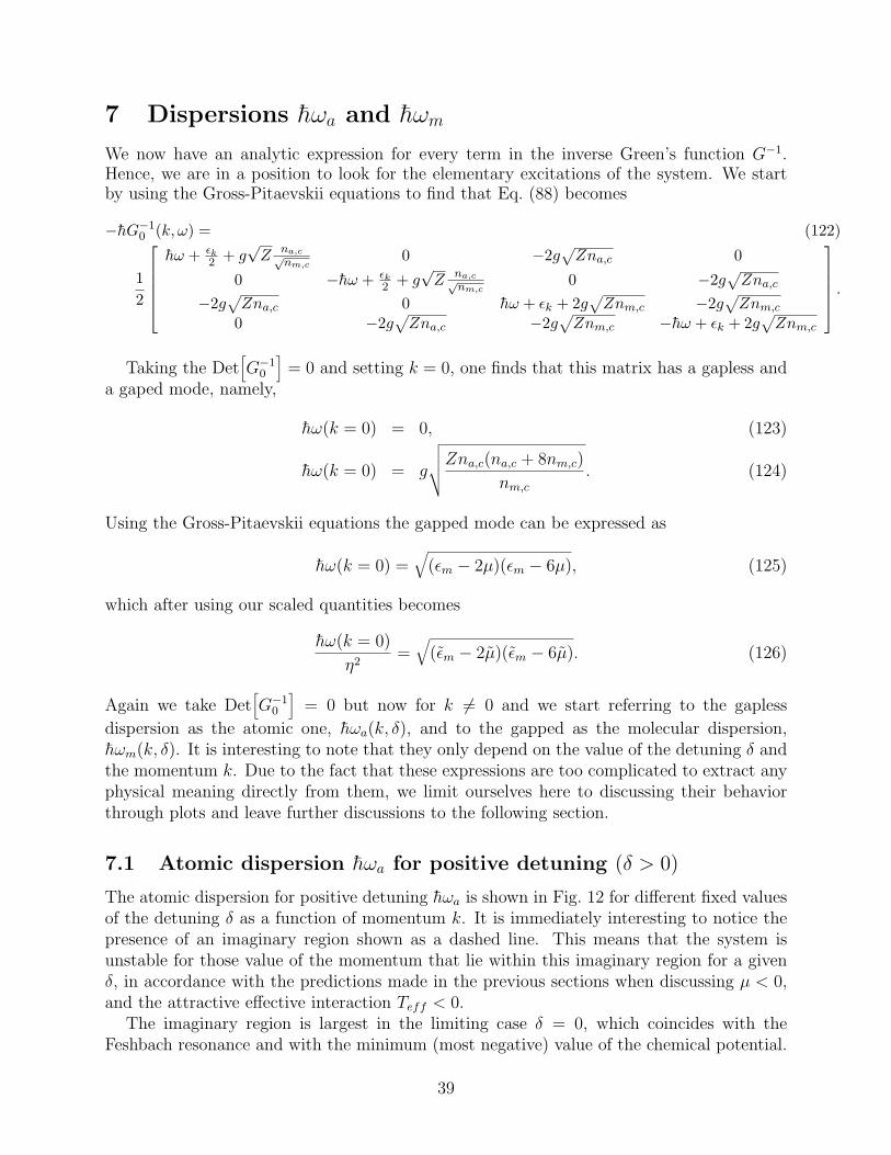
7.1 Atomic dispersion hωa for positive detuning (δ > 0)

The atomic dispersion for positive detuning hωa is shown in Fig. 12 for different fixed valuesof the detuning δ as a function of momentum k. It is immediately interesting to notice thepresence of an imaginary region shown as a dashed line. This means that the system isunstable for those value of the momentum that lie within this imaginary region for a givenδ, in accordance with the predictions made in the previous sections when discussing µ < 0,and the attractive effective interaction Teff < 0.

The imaginary region is largest in the limiting case δ = 0, which coincides with theFeshbach resonance and with the minimum (most negative) value of the chemical potential.

39

0.002 0.004 0.006 0.008

2Εk

Η

5106

0.00001

0.000015

0.00002

0.000025

0.00003

ΩaΗ2

Figure 12: hωa(k, δ > 0): plots for the values of thedetuning δ = 0.2, 0.02, 0.002, 0.0002. For δ = 0.2 theimaginary regions has practically disappeared, while forδ = 0.002 and δ = 0.0002 the dispersions are practicallythe same.

The value of the momentum k at which hωa becomes real is given by

hkreal(δ)√2m

=

√√√√√√Z(δ)g(−1 + 2nm,c(δ) +

√1 + 4nm,c(δ)− 12nm,c(δ)2)√

nm,c(δ). (127)

As shown in Fig. 13, the imaginary region closes fast as the detuning increases but approacheszero asymptotically. Be that as it may, for δ >> g

√nm,c the imaginary region has practically

disappeared, as predicted when discussing µ → 0 for δ >> g√nm,c and in accordance with

the usual atomic BEC. Moreover, for small values of the detuning it is almost constant, inagreement with Fig. 11 in which the plot of δ = 0.002 and δ = 0.0002 are practically equal.

Furthermore, as the detuning increases the dispersion shows an avoided crossing thatobeys

ka.c. =2

h

√√√√gm√Z (na,c − 2nm,c)√

nm,c. (128)

In terms of our scaled quantities one finds

hka.c(δ)

η√

2m=hka.c(δ)√

2m=

√√√√√2c√Z(δ)(1− 4nm,c(δ))√

nm,c(δ), (129)

which behaves as seen in Fig. 14 as a function of the detuning. In Fig. 15 the avoided crossingis clearly seen in the dispersion. The two asymptotes of the avoided crossing are

limk→∞

hωm(k, δ) =h2k2

2m+ 2g

√Z(δ)nm,c(δ), (130)

limk→∞

hωa(k, δ) =h2k2

4m+ gna,c(δ)

√√√√ Z(δ)

nm,c(δ). (131)

40

0.05 0.1 0.15 0.2

∆Η2

0.001

0.002

0.003

0.004

kreal2

m Η

Figure 13: kreal(δ): The imaginary part of the disper-sion closes very fast as the detuning increases. The insetshows how it is constant for small values of the detuning.

In our scaled quantitites this expresions become

limk→∞

hωm(k, δ)

η2=

h2k2

2m+ 2c

√Z(δ)nm,c(δ), (132)

limk→∞

hωa(k, δ)

η2=

h2k2

4m+ cna,c(δ)

√√√√ Z(δ)

nm,c(δ). (133)

It can be seen from these equations that within our approximation the avoided crossinghappens outside the imaginary region for every value of the detuning δ > 0. This may beclearly seen from their corresponding values at δ = 0, where using Z = 1, 4nm,c = na,c, nm,c =

1/6, and na,c = 2/3 they become ka.c. =2h

√gm√na.c. and kreal = 2

h

√gm(

√2−√na.c.). Since

na,c = 2/3 at δ = 0, clearly ka.c. > kreal for every δ > 0. Notice how if Z(δ) would have beencontinuous and vanish at δ = 0, we would have found hωm → εk and hωa → εk/2 in the limitk → ∞ at the Feshbach resonance. At the other limiting case for the detuning δ −→ ∞we see that ka.c. −→ ∞ and kreal −→ 0. Hence, we would expect the atomic dispersion toactually behave like the atomic gas dispersion for every value of k. Be that as it may, inthe limit k −→ ∞ one finds hωa −→ h2k2

4m+ gna,c

√Z

nm,c. From Eq. (88) it is clear that this

corresponds to the molecular part, in agreement with the above mentioned avoided crossing.The avoided crossing is due to the coupling between channels still present in G−1

0 at largedetuning, as can be seen in Eq. (109). Additionally, it should be noted that the unstableimaginary region disappears as the effective atomic chemical potential goes to zero, µa → 0,as mentioned in section 4.

7.2 Molecular dispersion hωm for positive detuning (δ > 0)

The molecular dispersion for positive detuning, shown in Fig. 16, has a gap given by Eq.(125)that grows as a function of the detuning, as shown in Fig. 17. In the limiting case δ = 0

41

0.002 0.004 0.006 0.008 0.01

∆Η2

0.006

0.008

0.012

0.014

kac2

m Η

Figure 14: kac(δ): Behaviour of the avoided crossing asa function of the detuning.

Figure 15: hωa(k, δ = 0.2): the dispersion shows anavoided crossing, shown in details in the inset.

42

the gap has its minimum value, which is given by hω0/η2 = 2c

√3. The dispersion hωm

also shows the avoided crossing mentioned above, and in this case in the limit k → ∞ it

becomes hωm −→ h2k2

2m+ 2g

√Znm,c. For large k the momentum term again dominates,

thus the dispersion becomes hωm −→ h2k2

2m= εk. This is the energy of a non-interacting

atom, which is what one would expect for large momentum, in agreement with the avoidedcrossing previously discussed, and with Eq. (109). Moreover, we see again that the coupling gin Hamiltonian has the effect of the avoided crossing between the two dispersions. Therefore,for δ >> g

√nm,c we find the dispersion of a non-interacting condensate of atoms with an

avoided crossing at infinity.

Figure 16: hωm(k, δ = 0.2): the molecular dispersionwith its avoided crossing shown in the inset.

0.00025 0.0005 0.00075 0.001 0.00125 0.0015

∆Η2

0.0000428

0.000043

0.0000432

0.0000434

0.0000436

0.0000438

0.000044

0.0000442

Ωm,0Η2

Figure 17: hωm,0(δ): the gap of the molecular dispersion.

43

7.3 Atomic dispersion hωa for negative detuning (δ < 0)

The atomic dispersion for negative detuning also has an imaginary region, as shown inFig. 18. Nevertheless, it differs from the positive detuning in its behavior because it vanishesat δ = 0, grows to a maximum value, and disappears again at δcrit. Its behavior is shown inFig. 19 and Fig. 20. Interestingly, the disappearance of the unstable imaginary region seemsto coincide with the effective molecular chemical potential having a zero value, µm = 0. Theimaginary region is indeed the instability predicted in the previous sections.

0.0005 0.001 0.0015 0.002

2Εk

Η

2107

4107

6107

8107

1106

1.2106

ΩaΗ2

Figure 18: hωa(k, δ < 0): the atomic dispersion for neg-ative detuning also shows an imaginary region (dottedlines). The three dispersions correspond to the valuesδ = −.002,−.004,−.008 correspondingly from left toright.

7.4 Molecular dispersion hωm for negative detuning (δ < 0)

The molecular dispersion for negative detuning is shown in Fig. 21. It has a gap that vanishesat δ = 0, starts increasing as δ increases negatively towards δcrit, but decreases back to zeroat δcrit as seen in Fig. 22. Therefore, hωm is gapless at the limits δ = 0 and δ = δcrit. Thatit is gapless for δ = 0 agrees with the previous discussion that at resonance one finds acondensate of atoms and gapless molecules.

After looking at the dispersion of the elementary excitations we have shown that theatomic dispersion has an imaginary region between 0 < k < kreal, which means it is unstable,as predicted previously. We have found an avoided crossing in the system at k = ka.c(δ).The asymptotes of the avoided crossing were specified and the behavior of the gap for themolecular dispersion explained. Thus, we now look for an expression for each dispersion thatmay let us see analytically the reason for the imaginary region.

44

0.00150.00125 0.001 0.000750.00050.00025

∆Η2

0.0002

0.0004

0.0006

0.0008

kreal2

m Η

Figure 19: kreal(δ): The size of the imaginary region interms of k as a function of the detuning is shown. At thevalues δ = 0 and δ = δcrit there is no imaginary region.

Figure 20: hωa(k, δ) close to the values of the detuningδ ≈ 0 and δ ≈ δcrit. The inset shows their imaginaryregions as short dashed lines.

45

0.0005 0.001 0.0015 0.002

2Εk

Η

5107

1106

1.5106

2106

2.5106

3106

ΩmΗ2

Figure 21: hωm(k, δ < 0) for different values of the detun-ing. The gap does not grow as for the positive detuningside.

0.00150.001250.0010.000750.00050.00025

∆Η2

2107

4107

6107

8107

1106

1.2106

Ωm,0Η2

Figure 22: hωm,o(δ < 0): the gap of the molecular dis-persion.

46

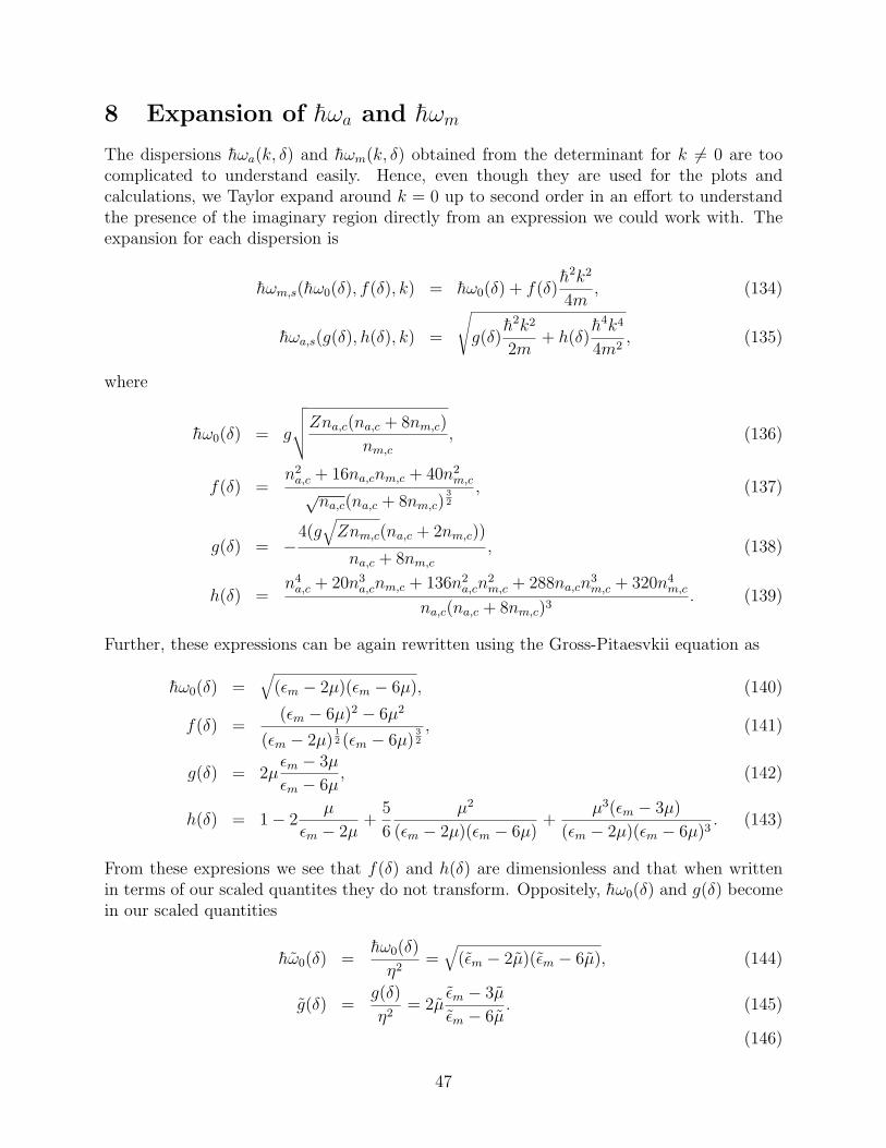
8 Expansion of hωa and hωm

The dispersions hωa(k, δ) and hωm(k, δ) obtained from the determinant for k 6= 0 are toocomplicated to understand easily. Hence, even though they are used for the plots andcalculations, we Taylor expand around k = 0 up to second order in an effort to understandthe presence of the imaginary region directly from an expression we could work with. Theexpansion for each dispersion is

hωm,s(hω0(δ), f(δ), k) = hω0(δ) + f(δ)h2k2

4m, (134)

hωa,s(g(δ), h(δ), k) =

√g(δ)

h2k2

2m+ h(δ)

h4k4

4m2, (135)

where

hω0(δ) = g

√√√√Zna,c(na,c + 8nm,c)

nm,c, (136)

f(δ) =n2a,c + 16na,cnm,c + 40n2

m,c√na,c(na,c + 8nm,c)

32

, (137)

g(δ) = −4(g

√Znm,c(na,c + 2nm,c))

na,c + 8nm,c, (138)

h(δ) =n4a,c + 20n3

a,cnm,c + 136n2a,cn

2m,c + 288na,cn

3m,c + 320n4

m,c

na,c(na,c + 8nm,c)3. (139)

Further, these expressions can be again rewritten using the Gross-Pitaesvkii equation as

hω0(δ) =√

(εm − 2µ)(εm − 6µ), (140)

f(δ) =(εm − 6µ)2 − 6µ2

(εm − 2µ)12 (εm − 6µ)

32

, (141)

g(δ) = 2µεm − 3µ

εm − 6µ, (142)

h(δ) = 1− 2µ

εm − 2µ+

5

6

µ2

(εm − 2µ)(εm − 6µ)+

µ3(εm − 3µ)

(εm − 2µ)(εm − 6µ)3. (143)

From these expresions we see that f(δ) and h(δ) are dimensionless and that when writtenin terms of our scaled quantites they do not transform. Oppositely, hω0(δ) and g(δ) becomein our scaled quantities

hω0(δ) =hω0(δ)

η2=√

(εm − 2µ)(εm − 6µ), (144)

g(δ) =g(δ)

η2= 2µ

εm − 3µ

εm − 6µ. (145)

(146)

47

Thus, the expansions become

hωm,s(hω0(δ), f(δ), k)

η2= hω0(δ) + f(δ)

h2k2

4m, (147)

hωa,s(g(δ), h(δ), k)

η2=

√g(δ)

h2k2

2m+ h(δ)

h4k4

4m2, (148)

Let us now look how these four functions behave at the different limits of the detuningto try to understand the behavior of the dispersions discussed in the previous section.

8.1 Expansion of atomic dispersion hωa,s for positive detuning.

0.02 0.04 0.06 0.08

∆Η2

0.000012

0.00001

8106

6106

4106

2106

gΗ2

Figure 23: The function g(δ) resembles the chemical po-tential for positive detuning.

Starting with the function g(δ) we see that for large positive detuning it goes to zero.From our previous discussion of µ we realize that if we analyze the function by parts theybecome

µ −→ 0, (149)εm − 3µ

εm − 6µ−→ 1.

Therefore, the function g(δ) −→ 0 for large positive detuning, because the chemical potentialalso increases µ −→ 0. Its behaviour is shown in Fig. 23.

Looking now at the function h(δ), shown in Fig. 24, we see that for large positive detuningδ >> g

√nm,c the function reduces onto

h(δ) −→ h(δ) ≈ 1− 2nm,cna,c

+5

6

(nm,cna,c

)2

−(nm,cna,c

)3

. (150)

48

0.01 0.02 0.03 0.04

∆Η2

0.75

0.8

0.85

0.9

0.95

h

Figure 24: The dimensionless function na,c(δ)h(δ) thatmultiplies the ε2k term has the effect of scaling it downclose to the Feshbach resonance.

Further, since the ratio between the densities nm,c

na,c≈ 0, we see that for large positive detuning

the function h(δ) ≈ e−2nm,c/na,c → 1, considering only up to linear terms in the ratio of thecondensate densities.

Thus, at large positive detuning where g(δ) −→ 0 and h(δ) −→ 1 the expansion of theatomic dispersion becomes

hωa,s(g(δ), h(δ), k)|δ>>g√nm,c=h2k2

2m. (151)

Therefore, for large values of the detuning, the atomic dispersion becomes the dispersion ofa free atomic gas, which means it does not support the avoided crossing and is thus valid atbest up to the value of the momentum ka.c., but it agrees with the value of hωm after theavoided crossing.

We are thus left with the task of explaining the imaginary region of the dispersion for lowervalues of the detuning close to δ ↓ 0. Again let us start by looking at the g(δ) function in itsform Eq. (142) that takes the simple form g(0) = µ < 0. Similarly, using that 4nm,c = na,cat δ = 0, the function h(δ) becomes h(0) = 3/4. Hence, the dispersion at the Feshbachresonance is

hωa,s(g(δ), h(δ), k)|δ=0 =

√µεk +

3

4ε2k. (152)

One clearly sees that both the εk and the ε2k terms are scaled down at resonance and thatthe imaginary unstable part is due to the negative sign of µ. Thus, we realize that for valuesof the momenta k < kreal one has |µεk| > |3

4ε2k|. In addition, we have seen that the chemical

potential is always negative, hence what determines whether g(δ) < 0 for all δ > 0 andmakes the dispersion imaginary comes from the sign of the factor

εm − 3µ

εm − 6µ. (153)

49

We see that even though they are the difference between the binding energy and the chemicalpotential they are effectively a sum, because of the negative value of µ and εm(δ) > 0 forpositive detuning. Thus, there are no poles in the denominator. Furthermore, the valuesof both the numerator and the denominator are always positive, which makes g(δ) < 0 forall values of the detuning due to µ < 0. We may therefore generalize |g(δ)εk| > |h(δ)ε2k|for k < kreal. Additionally, the function g(δ) may be regarded as the chemical potential µthat scales as a function of the detuning. This also explains why the imaginary region closesasymptotically as µ asymptotically approaches zero.

8.2 Expansion of molecular dispersion hωm,s for positive detuning.

Starting with the gap hω0 one sees that for large values of the detuning (δ >> g√nm,c) the

chemical potential tends to zero and it becomes hω0 −→ εm(δ). Hence, hω0 indeed divergesas the binding energy diverges as a function of the detuning. On the other hand, as can beseen in Fig. 25, the function f(δ) for large detuning becomes one because as the chemical

potential increases to zero it becomes f(δ) −→ ε2mε2m

. Thus, the expansion of the moleculardispersion becomes

hωm,s(hω0(δ), f(δ), k)|δ>>g√nm,c= εm +

h2k2

4m, (154)

which is the non-interacting molecular dispersion. Therefore, one concludes that just as forthe atomic dispersion the expansion of hωm is valid at best up to the value of the momentumof the avoided crossing ka.c..

0.005 0.01 0.015 0.02 0.025 0.03

∆Η2

1.1

1.2

1.3

1.4

f

Figure 25: The dimensionless function f(δ) amplifies thekinetic term in the molecular dispersion. Notice how itseffect is strongest at resonance.

On the limiting case δ ↓ 0 the gap reduces to its minimum value, hω0 = 2√

3|µ|. This valueis positive because the minus sign of the chemical potential was lost when it was squared inEq.(138). On the other hand, the function f(δ) has its maximum value at this value of thedetuning, f(0) = 5/2

√3. This makes the molecular dispersion become

50

hωm,s(hω0(δ), f(δ), k)|δ=0 = 2√

3|µ|+ 5

2√

3

h2k2

4m. (155)

Hence, it seems the kinetic part of the molecular dispersion is enhanced as the detuningdecreases from δ >> g

√nm,c to δ → 0.

8.3 Expansion of atomic dispersion hωa,s for negative detuning.

Again we analyze hωa,s. Looking first at the case δ = 0 we see that the function g(δ) vanishesbecause at δ = 0 the chemical potential vanishes (µ = 0), as shown in Fig. 26. Notice howthis differs from the positive detuning value, as discussed for the chemical potential, due to Z.On the other hand, the function h(δ) is continuous at the Feshbach resonance, h(0) = 3/4,clearly because it does not depend on Z. It is plotted in Fig. 27. This gives the atomicdispersion at δ = 0 on the negative detuning side,

hωa,s(g(δ), h(δ), k)|δ=0 =

√3

4εk, (156)

which is indeed the dispersion of a non-interacting atomic gas.

0.00150.00125 0.001 0.000750.00050.00025

∆Η2

6107

5107

4107

3107

2107

1107

gΗ2

Figure 26: The function g(δ) for δ < 0. It is alwaysnegative due to its dependence on µ.

Turning now to the critical point δcrit, we know that εm(δcrit) = 2µ(δcrit) and nm,c = 12.

These give g(δcrit) = µ/2, and h(δcrit) →∞. Thus, the function h(δ) that multiplies the termε2k scales it up and eventually makes the atomic dipsersion diverge as the detuning approachesδcrit. This is not the case, since we know that the atomic dispersion does not diverge at δcrit.Additionally, the function g(δ) could still be seen as a scaled chemical potential.

8.4 Expansion of molecular dispersion hωm,s for negative detuning.

Just as in the full dispersion, the gap of the expansion, hω0, closes at both δ = 0, andδ = δcrit. For the same reasons as before, hω0(0) = 0 because εm(0) = 0, and µ(0) = 0, while

51

0.0015 0.00125 0.001 0.00075 0.0005 0.00025

∆Η2

5

10

15

20

h

Figure 27: The dimensionless function h(δ) also scalesdown the ε2k term for negative detuning. Notice that thedivergence of h(δ) at δcrit means that the expansion isnot valid close to this value of the detuning.

the gap hω0(δcrit) = 0 because εm(δcrit) = 2µ(δcrit) as previously mentioned. Looking now atthe function f(δ), shown in Fig. 28, we see that at δ = 0 it becomes f(δ) = 5/2

√3 like for

the positive detuning side. Hence, f(δ) is continuous at the Feshbach resonance because itdoes not depend on Z. This gives the molecular dispersion

hωm,s(ω0(δ), f(δ), k)|δ=0 =5

2√

3

εk2, (157)

which is indeed gapless as previously seen for the full molecular dispersion and is a non-interacting atomic dispersion. In addition, contrary to hω0(δcrit) that vanishes, the functionf(δ) at the critical point diverges, f(δcrit) → ∞. This is caused by εm = 2µ at this valueof the detuning. We know that the molecular dispersion does not diverge at the quantumcritical point. In addition, we see that throughout the negative values of the detuningconsidered in our discussion, the kinetic part of the molecular dispersion is multiplied by thefunction f(δ), which has the effect of amplifying it.

8.5 Comparison of atomic expansion with Bogoliubov theory

We now want to see how the expansion of the atomic dispersion compares to the Bogoliubovone. We know that

hωB =√εk (εk + 2V0n0). (158)

The expansion of the atomic dispersion can be written as

hωa,s =

√√√√h(δ)εk(εk +

g(δ)

h(δ)

). (159)

52

0.00150.00125 0.001 0.000750.00050.00025

∆Η2

2.5

5

7.5

10

12.5

15

17.5

f

Figure 28: The dimensionaless function f(δ) that mul-tiplies the kinetic term of the molecular dispersion alsohas a magnifying effect for negative detuning. Notice inthe inset how f(δ) is divergent if it is not multiplied byna,c.

Comparing both expression one sees that

2V0n0 −→g(δ)

h(δ). (160)

As shown in Fig. 29 and in Fig. 30, the ratio g/h is negative for every value of the detuningwhere an atomic condensate is present. Hence, from our comparison with the Bogoliubovdispersion shows that we have effectively attractive interactions, which as mentioned beforeresult in an unstable condensate that collapses into itself. Considering again g(δ) as a scaledchemical potential, we again conclude that its negative value results in the instability of thesystem.

So far we have shown in this section that the Taylor expansion of the dispersions aroundk = 0 are given by

hωm,s(hω0(δ), f(δ), k) = hω0(δ) + f(δ)h2k2

4m, (161)

hωa,s(g(δ), h(δ), k) =

√g(δ)

h2k2

2m+ h(δ)

h4k4

4m2. (162)

Also, we showed that for the atomic dispersion the function g(δ) is basically the scaled chem-ical potential. Thus, the imaginary regions arises because µ < 0. We have also shown thatthe function h(δ) scales down the quadratic kinetic term ε2k, while the function f(δ) multipliesthe kinetic term. In addition, we have argued that the expansions do not accurately describethe behaviour close to the quantum critical point, since the full dispersions do not divergeat this value of the detuning. We may extend this argument for positive detuning because

53

0.000150.0001250.00010.0000750.000050.000025

∆Η2

2.5107

2107

1.5107

1107

5108

ghΗ2

Figure 29: The factor g(δ)/h(δ) is always negative forδ < 0, which results in an unstable condensate.

the expansions do not show the avoided crossing. Thus, the avoided crossing is outside theregion of validity of the expansion. Hence, both for positive and negative detuning, the ex-pansions around k = 0 do not hold for every value of the detuning. The problem presumablyarises because in the full dispersions their is a change of behaviour as the dominant k termchanges from linear to quadratic, which takes place for a different value of k depending onthe detuning. This change of behaviour is not described by the expansions. Certainly thepresence of the imaginary region and instability of the system are the more pressing issuesto clarify and discuss. In order to further look into it and see how the system may becomestable we look now at the eigenvalues of the energy of the ground state.

54

0.01 0.02 0.03 0.04 0.05

∆Η2

0.000015

0.0000125

0.00001

7.5106

5106

2.5106

ghΗ2

Figure 30: The factor g(δ)/h(δ) is always negative forδ > 0, and becomes zero only at large detuning. Hence,the system is unstable, as expected for positive detuning.

55

9 Eigenvalues and Stability

The question that now arises is whether the system can be stable at all. To approach thisproblem we first ascertain if the energy in the ground state is positive definite by the second-derivate test. Secondly, we look at the eigenvalues of the resulting Hessian matrix and studythe effect of the nonresonant interactions Tij. Finally, we find conditions for the values ofTij required to make the system stable.

9.1 Second-derivative test of the energy.

Being more precise, it is not the second derivative test of the energy, but rather of the freeenergy because it is the free energy that is at a minimum as discussed in section 2.3. Atthe moment we have the grand canonical potential Ω = E − TS − µN , which for the zerotemperature calculation we are doing reduces to Ω = E − µN . Hence, the energy is givenby E(N) = Ω + µN , i.e.,

ε =E

V= εmnm,c − 2g

√Zna,cn

1/2m,c +

Tmm2

n2m,c + Tamnm,cna,c +

Taa2n2a,c, (163)

where there are no kinetic terms because of the boson’s ground state k = 0, and V is thevolume of the system, that is to say, we actually have the energy density of the system ε.The second derivative test now consists of finding the Hessian matrix

∑i,j

det

[∂ε

∂ni∂nj

]ij

≥ 0, (164)

where i, j = 1, 2 means atomic and molecular condensate respectively. Clearly, in our mean-field approach taking the partial derivative with respect to the condensate density is equiv-alent to doing the derivative with respect to the mean-field value of the field in the groundstate, 〈ψi〉 =

√ni,c. The resulting matrix is

∑i,j

[∂ε

∂ni∂nj

]i,j

=

Taa −g√

Znm,c

+ Tam

−g√

Znm,c

+ Tam12g na,c

nm,c

√Znm,c + Tmm

. (165)

If we diagonalize the Hessian matrix before taking the determinant, i.e.,

det

[ ∂ε

∂ni∂nj

]ij

− λI

= 0, (166)

we find the determinant is given by

(1

2gna,cnm,c

√Znm,c + Tmm − λ

)(Taa − λ)−

(Tam − g

√Z

nm,c

)2

= 0. (167)

Let us now solve this equation and see how the energy density eigenvalues behave.

56

9.2 Eigenvalues Considering the nonresonant Interactions Tij In-dividually

We know that the stability condition requires the two eigenvalues to be positive. Let us startby defining the eigenvalues λ1,2 from the free energy resulting from the resonant HamiltonianH0 and then see how the different terms of Hint affect it. The eigenvalues for Tij = 0 aregiven by

λ1,2 =1

4nm,c

(gna,c

√Z

nm,c±√g2n2

a,c

Z

nm,c+ 16g2nm,cZ

). (168)

Using the Gross-Pitaevskii equations they can be written as

0.00150.00125 0.001 0.000750.00050.00025

∆Η2

1106

5107

5107

1106

1.5106

2106

nT Λ1,2Η2

Figure 31: Behavior of the two eigenvalues without Tijas a function of detuning for δ < 0.

0.001 0.002 0.003 0.004 0.005 0.006

∆Η2

0.0001

0.0002

0.0003

0.0004

nT Λ1,2Η2

Figure 32: Behavior of the two eigenvalues without Tijas a function of detuning for δ > 0.

λ1,2 =1

4nm,c

((εm − 2µ)±

√(εm − 2µ)2 + 4µ2

), (169)

57

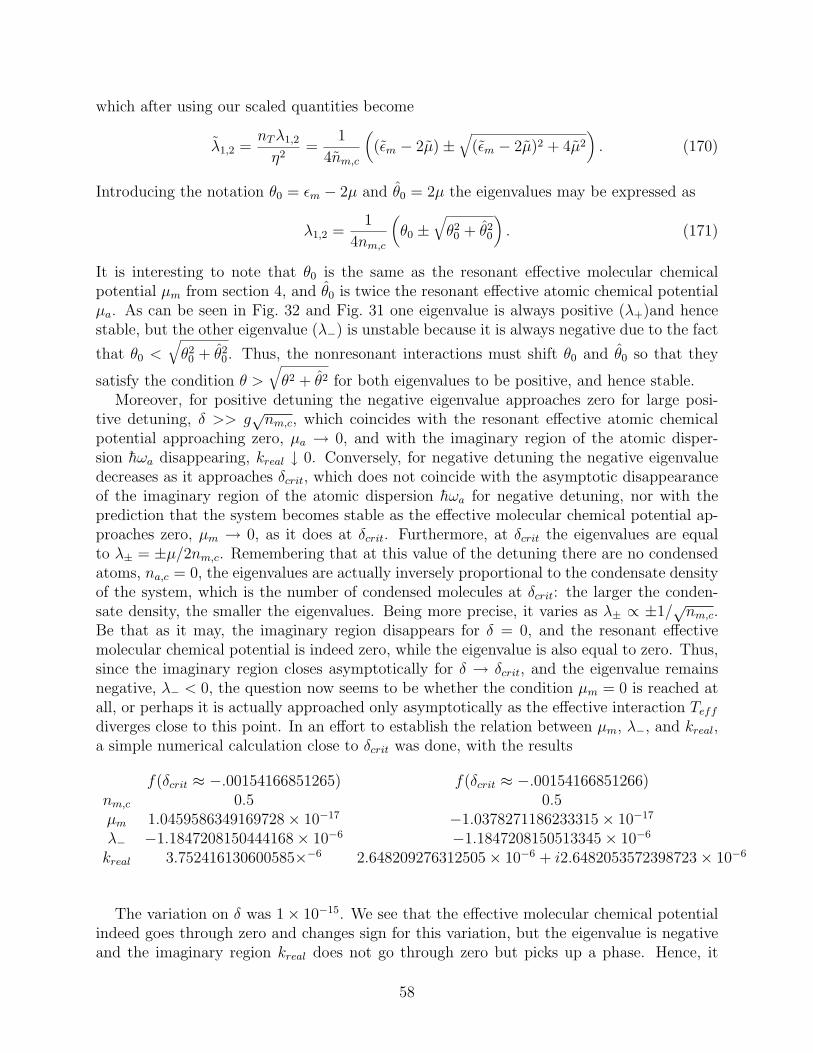
which after using our scaled quantities become

λ1,2 =nTλ1,2

η2=

1

4nm,c

((εm − 2µ)±

√(εm − 2µ)2 + 4µ2

). (170)

Introducing the notation θ0 = εm − 2µ and θ0 = 2µ the eigenvalues may be expressed as

λ1,2 =1

4nm,c

(θ0 ±

√θ20 + θ2

0

). (171)

It is interesting to note that θ0 is the same as the resonant effective molecular chemicalpotential µm from section 4, and θ0 is twice the resonant effective atomic chemical potentialµa. As can be seen in Fig. 32 and Fig. 31 one eigenvalue is always positive (λ+)and hencestable, but the other eigenvalue (λ−) is unstable because it is always negative due to the fact

that θ0 <√θ20 + θ2

0. Thus, the nonresonant interactions must shift θ0 and θ0 so that they

satisfy the condition θ >√θ2 + θ2 for both eigenvalues to be positive, and hence stable.

Moreover, for positive detuning the negative eigenvalue approaches zero for large posi-tive detuning, δ >> g

√nm,c, which coincides with the resonant effective atomic chemical

potential approaching zero, µa → 0, and with the imaginary region of the atomic disper-sion hωa disappearing, kreal ↓ 0. Conversely, for negative detuning the negative eigenvaluedecreases as it approaches δcrit, which does not coincide with the asymptotic disappearanceof the imaginary region of the atomic dispersion hωa for negative detuning, nor with theprediction that the system becomes stable as the effective molecular chemical potential ap-proaches zero, µm → 0, as it does at δcrit. Furthermore, at δcrit the eigenvalues are equalto λ± = ±µ/2nm,c. Remembering that at this value of the detuning there are no condensedatoms, na,c = 0, the eigenvalues are actually inversely proportional to the condensate densityof the system, which is the number of condensed molecules at δcrit: the larger the conden-sate density, the smaller the eigenvalues. Being more precise, it varies as λ± ∝ ±1/

√nm,c.

Be that as it may, the imaginary region disappears for δ = 0, and the resonant effectivemolecular chemical potential is indeed zero, while the eigenvalue is also equal to zero. Thus,since the imaginary region closes asymptotically for δ → δcrit, and the eigenvalue remainsnegative, λ− < 0, the question now seems to be whether the condition µm = 0 is reached atall, or perhaps it is actually approached only asymptotically as the effective interaction Teffdiverges close to this point. In an effort to establish the relation between µm, λ−, and kreal,a simple numerical calculation close to δcrit was done, with the results

f(δcrit ≈ −.00154166851265) f(δcrit ≈ −.00154166851266)nm,c 0.5 0.5µm 1.0459586349169728× 10−17 −1.0378271186233315× 10−17

λ− −1.1847208150444168× 10−6 −1.1847208150513345× 10−6

kreal 3.752416130600585×−6 2.648209276312505× 10−6 + i2.6482053572398723× 10−6

The variation on δ was 1× 10−15. We see that the effective molecular chemical potentialindeed goes through zero and changes sign for this variation, but the eigenvalue is negativeand the imaginary region kreal does not go through zero but picks up a phase. Hence, it

58

seems that, as seen in the expansion of the atomic dispersion, the imaginary unstable partdoes not vanish at δcrit. We now look at how the interactions modify these eigenvalues inorder to see if the negative eigenvalue is shifted to the positive side.

9.2.1 Atom-Atom interaction, Taa 6= 0

We start by setting Taa 6= 0. In this case the eigenvalues become

λ± =1

4nm,c

(θ0 + 2nm,cTaa ±

√(θ0 + 2nm,cTaa)2 + (θ2

0 − 8gna,c√Znm,cTaa)

). (172)

The stability condition is satisfied when

θ20 − 8gna,c

√Znm,cTaa ≤ 0. (173)

Solving for Taa one finds

Taa ≥2g2Z

εm − 2µ= −Teff . (174)

Since Taa depends on the background scattering length abg it does not depend on thedetuning. It is constant as mentioned in section 3.2. Consequently, we consider repulsiveinteractions Taa > 0 for every value of the detuning. Thus, Taa > 0 helps make the negativeeigenvalue turn into a positive one, provided that the effective molecular chemical potentialis negative as in the resonant case. Clearly, Taa scales as Teff , and should counteract theeffect of the resonant interaction. The lower bound is shown in Fig. 33.

0.0014 0.0012 0.001 0.0008 0.0006 0.0004 0.0002

∆Η2

1106

2106

3106

4106

5106

TnTΗ2

Figure 33: For δ < 0: Above the solid line is the regionof stability of Taa, and below the dashed line is the re-gion of stability of Tam. Notice how Taa diverges as itapproaches δcrit, contrary to Tam that remains finite andrather constant.

59

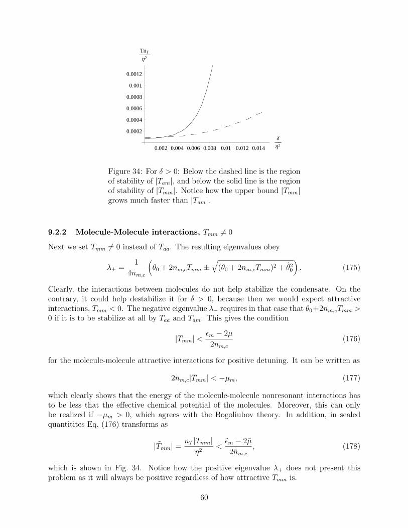
0.002 0.004 0.006 0.008 0.01 0.012 0.014

∆Η2

0.0002

0.0004

0.0006

0.0008

0.001

0.0012

TnTΗ2

Figure 34: For δ > 0: Below the dashed line is the regionof stability of |Tam|, and below the solid line is the regionof stability of |Tmm|. Notice how the upper bound |Tmm|grows much faster than |Tam|.

9.2.2 Molecule-Molecule interactions, Tmm 6= 0

Next we set Tmm 6= 0 instead of Taa. The resulting eigenvalues obey

λ± =1

4nm,c

(θ0 + 2nm,cTmm ±

√(θ0 + 2nm,cTmm)2 + θ2

0

). (175)

Clearly, the interactions between molecules do not help stabilize the condensate. On thecontrary, it could help destabilize it for δ > 0, because then we would expect attractiveinteractions, Tmm < 0. The negative eigenvalue λ− requires in that case that θ0+2nm,cTmm >0 if it is to be stabilize at all by Taa and Tam. This gives the condition

|Tmm| <εm − 2µ

2nm,c(176)

for the molecule-molecule attractive interactions for positive detuning. It can be written as

2nm,c|Tmm| < −µm, (177)

which clearly shows that the energy of the molecule-molecule nonresonant interactions hasto be less that the effective chemical potential of the molecules. Moreover, this can onlybe realized if −µm > 0, which agrees with the Bogoliubov theory. In addition, in scaledquantitites Eq. (176) transforms as

|Tmm| =nT |Tmm|

η2<εm − 2µ

2nm,c, (178)

which is shown in Fig. 34. Notice how the positive eigenvalue λ+ does not present thisproblem as it will always be positive regardless of how attractive Tmm is.

60

9.2.3 Atom-Molecule interaction, Tam 6= 0

Finally, we look at Tam 6= 0 while all the other Tii = 0. One thus gets the eigenvalues

λ± =1

4nm,c

θ0 ±

√√√√θ20 + (θ2

0 − 16n2m,c(2g

√Z

nm,cTam + T 2

am))

. (179)

Solving the quadratic equation θ20 − 16n2

m,c(2g√

Znm,c

Tam + T 2am) = 0 for Tam one finds

(Tam + g

√Z

nm,c(1−

√2))(Tam + g

√Z

nm,c(1 +

√2)) ≤ 0. (180)

Being aware of the same change in the scattering length for positive and negative detuning,and its effect in changing the interactions from attractive to repulsive correspondingly, weonce more introduce the absolute value of the scattering,

(±|Tam| − g

√Z

nm,c(√

2− 1))(±|Tam|+ g

√Z

nm,c(1 +

√2)) ≤ 0. (181)

Requiring that Tam > 0 in order to have repulsive interactions for δ < 0 means that thesecond term of the product in Eq. (181) is always positive. That leaves only the first termto try to fulfill the condition (180). As shown in Fig. 33, this is achieved by the followinginterval of the scattering amplitude between an atom and a molecule

0 < |Tam| < (√

2− 1)g

√Z

nm,c. (182)

Writing this condition in scaled quantites we find

0 <nT |Tam|η2

< (√

2− 1)c

√Z

nm,c. (183)

Therefore, the interactions between an atom and a molecule also help stabilize the con-densate for negative detuning, where interactions are repulsive, Tam > 0. For attractiveinteractions, Tam < 0, we realize that the condition for stability, Eq. (181), now becomes

(|Tam|+ g

√Z

nm,c(√

2− 1))(|Tam| − g

√Z

nm,c(1 +

√2)) ≤ 0. (184)

Now the first term is always positive, and only the second terms could satisfy the inequality.This is achieved when

0 < |Tam| < (√

2 + 1)g

√Z

nm,c, (185)

which is shown is Fig. 34. In scaled quantities becomes

0 <nT |Tam|η2

< (√

2 + 1)c

√Z

nm,c. (186)

61

9.2.4 Relation between Taa and Tam

Although precise analytic expressions for the Tii matrices are not readily available, they canbe measured in experiments. Therefore, we look at the ratio between the lower bound of Taaand the upper bound of Tam in order to get the following expression

TaaTam

≥ 1√2∓ 1

2nm,cna,c

, (187)

where the ∓ on the right hand side takes into account the change from repulsive (-) toattractive (+) interactions of Tam depending on the detuning. Clearly, the inequality dependsonly on the ratio between the condensate densities between species as a function of thedetuning. Hence, the stability of the system depends on the ratio the condensate densities ofmolecules and atoms. Consequently, not only the ratio between the condensate densities ofatoms and molecules varies as a function of detunning, also the ratio between atom-atom andatom-molecule interactions. For instance, na,c(δcrit) = 0 implies Tam|δcrit

= 0. For differentvalues of the detuning one finds that the ratio between nonresonant interactions varies asseen in the table below

1√2+1

2nm,c

na,c< 1 Taa < Tam δ > 0

1√2+1

2nm,c

na,c= 1 Taa = Tam δ > 0

1√2∓1

2nm,c

na,c> 1 Taa > Tam δ < 0, δ > 0

.

Provided we know Taa, we could then find that Tam should obey

Tam ≤ (√

2∓ 1)na,c

2nm,cTaa. (188)

In addition, using the expressions for Taa = (4πabgh2)/2m and Tam = (4πaamh

2)/3m in termsof the atomic scattering length found in Ref. [9] for zero external momentum and frequencyclose to resonance, aam = 32a/3, the stability condition Eq. (188) close to resonance is foundto be

abga≥ 128

9(√

2∓ 1)

nm,cna,c

, (189)

which clearly shows that we must have nm,c << na,c at the Feshbach resonance, since theratio abg/a→ 0 as the scattering length diverges at δ ≈ 0.

9.3 Eigenvalues Considering the nonresonant Interactions Tij thatIndividually Stabilized the System

Considering that in the Bose gas all the interactions take place at the same time, we nowwant to see how the interactions Tij that individually help stabilized the system relate toeach other.

62

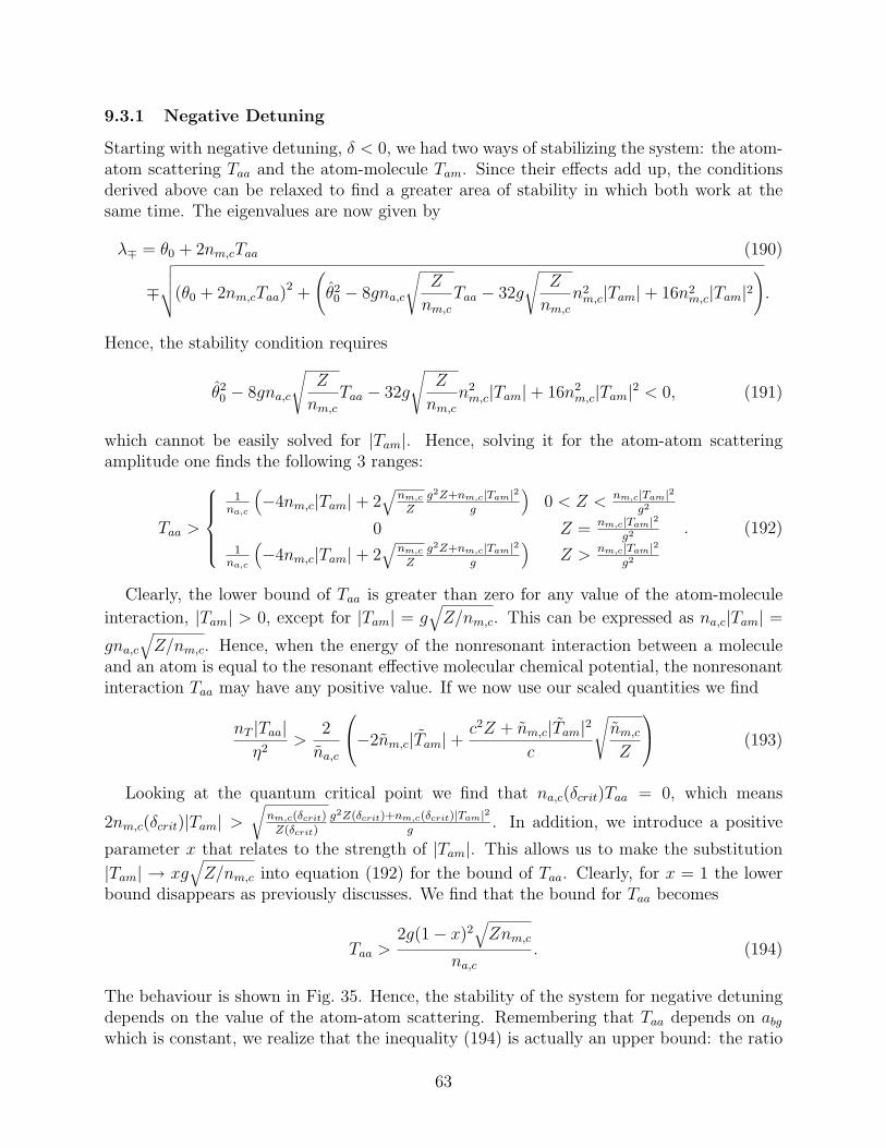
9.3.1 Negative Detuning

Starting with negative detuning, δ < 0, we had two ways of stabilizing the system: the atom-atom scattering Taa and the atom-molecule Tam. Since their effects add up, the conditionsderived above can be relaxed to find a greater area of stability in which both work at thesame time. The eigenvalues are now given by

λ∓ = θ0 + 2nm,cTaa (190)

∓

√√√√(θ0 + 2nm,cTaa)2 +

(θ20 − 8gna,c

√Z

nm,cTaa − 32g

√Z

nm,cn2m,c|Tam|+ 16n2

m,c|Tam|2).

Hence, the stability condition requires

θ20 − 8gna,c

√Z

nm,cTaa − 32g

√Z

nm,cn2m,c|Tam|+ 16n2

m,c|Tam|2 < 0, (191)

which cannot be easily solved for |Tam|. Hence, solving it for the atom-atom scatteringamplitude one finds the following 3 ranges:

Taa >

1na,c

(−4nm,c|Tam|+ 2

√nm,c

Zg2Z+nm,c|Tam|2

g

)0 < Z < nm,c|Tam|2

g2

0 Z = nm,c|Tam|2g2

1na,c

(−4nm,c|Tam|+ 2

√nm,c

Zg2Z+nm,c|Tam|2

g

)Z > nm,c|Tam|2

g2

. (192)

Clearly, the lower bound of Taa is greater than zero for any value of the atom-molecule

interaction, |Tam| > 0, except for |Tam| = g√Z/nm,c. This can be expressed as na,c|Tam| =

gna,c√Z/nm,c. Hence, when the energy of the nonresonant interaction between a molecule

and an atom is equal to the resonant effective molecular chemical potential, the nonresonantinteraction Taa may have any positive value. If we now use our scaled quantities we find

nT |Taa|η2

>2

na,c

−2nm,c|Tam|+c2Z + nm,c|Tam|2

c

√nm,cZ

(193)

Looking at the quantum critical point we find that na,c(δcrit)Taa = 0, which means

2nm,c(δcrit)|Tam| >√

nm,c(δcrit)Z(δcrit)

g2Z(δcrit)+nm,c(δcrit)|Tam|2g

. In addition, we introduce a positive

parameter x that relates to the strength of |Tam|. This allows us to make the substitution

|Tam| → xg√Z/nm,c into equation (192) for the bound of Taa. Clearly, for x = 1 the lower

bound disappears as previously discusses. We find that the bound for Taa becomes

Taa >2g(1− x)2

√Znm,c

na,c. (194)

The behaviour is shown in Fig. 35. Hence, the stability of the system for negative detuningdepends on the value of the atom-atom scattering. Remembering that Taa depends on abgwhich is constant, we realize that the inequality (194) is actually an upper bound: the ratio

63

between condensate molecules and condensate atoms, and their nonresonant interactions,which we parametrized with x, must be less than Taa for the system to be stable. This bound

becomes zero when na,c|Tam| = gna,c√Z/nm,c, which is the resonant effective molecular

potential, or equivalently when nm,c|Tam| = g√Znm,c, which up to a factor of two is the

resonant effective atomic chemical potential. Moreover, Eq. (194) cam be written as na,cTaa >−(1− x)2µa,0, where µa,0 is the resonant effective atomic chemical potential. Hence, for thesystem to be stable the effective atomic chemical potential has to become positive whenincluding the nonresonant Taa. This can be seen in Fig. 36 where equation (194) is shownfor different values of the detuning and the parameter x.

Figure 35: Lower bound of Taa for the gas to be stable.The dashed line is for x = 0.8 and the solid line is forx = 1.4. Notice how Taa is not required to diverge atthe Feshbach resonance, while it is required to do so atthe quantum critical point. The inset shows the energybound for the background scattering.

9.3.2 Positive Detuning

Now we look at positive detuning. In that case we found that apparently the atom-moleculeand the atom-atom interactions help stabilize the system. Surprisingly, it is the combinationof −|Tmm| and Taa that helps stabilize the system by setting a bound on |Tmm|, while Taamay have any value, and |Tam| has a non trivial solution due to the fact that it is quadratic.Noticing that |Tmm| may again destabilize the system just as when analyzing Tmm individ-ually, let us start by setting |Tam| = 0 and study its individual behaviour. In this case theeigenvalues are given by

λ∓ = θ0 + 2nm,cTaa − 2nm,c|Tmm| (195)

64

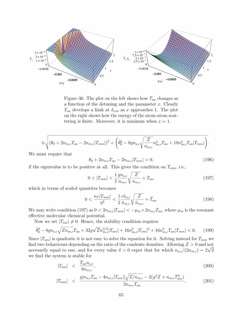
x

2d/h

Taa T naa a,c

2d/h

x

Figure 36: The plot on the left shows how Taa changes asa function of the detuning and the parameter x. ClearlyTaa develops a kink at δcrit as x approaches 1. The ploton the right shows how the energy of the atom-atom scat-tering is finite. Moreover, it is minimun when x = 1.

∓

√√√√(θ0 + 2nm,cTaa − 2nm,c|Tmm|)2 +

(θ20 − 8gna,c

√Z

nm,cn2m,cTaa + 18n2

m,cTaa|Tmm|).

We must require thatθ0 + 2nm,cTaa − 2nm,c|Tmm| > 0, (196)

if the eigenvalue is to be positive at all. This gives the condition on Tmm, i.e.,

0 < |Tmm| <1

2

gna,cnm,c

√Z

nm,c+ Taa, (197)

which in terms of scaled quantites becomes

0 <nT |Tmm|

η2<

1

2

cna,cnm,c

√Z

nm,c+ Taa. (198)

We may write condition (197) as 0 < 2nm,c|Tmm| < −µm+2nm,cTaa, where µm is the resonanteffective molecular chemical potential.

Now we set |Tam| 6= 0. Hence, the stability condition requires

θ20 − 8gna,c

√Znm,cTaa + 32g

√Zn3/2

m,c|Tam|+ 16n2m,c|Tam|2 + 16n2

m,cTaa|Tmm| < 0. (199)

Since |Tam| is quadratic it is not easy to solve the equation for it. Solving instead for Tmm wefind two behaviours depending on the ratio of the condente densities. Allowing Z > 0 and notnecesarily equal to one, and for every value δ > 0 expet that for which na,c/(2nm,c) = 2

√2

we find the system is stable for

|Tam| <Taana,c8nm,c

, (200)

|Tmm| <g|na,cTaa − 4nm,c|Tam||

√Z/nm,c − 2(g2Z + nm,cT

2am)

2nm,cTaa, (201)

65

and

8n2m,c|Tam|2 + na,cTaa(na,cTaa − 8nm,c|Tam|)− |na,cTaa − 4nm,c|Tam||

√na,cTaa(na,cTaa − 8nm,c|Tam|)

< 8g2Znm,c < (202)

8n2m,c|Tam|2 + na,cTaa(na,cTaa − 8nm,c|Tam|) + |na,cTaa − 4nm,c|Tam||

√na,cTaa(na,cTaa − 8nm,c|Tam|).

The condition may be written in terms of our scaled quantities, i.e.,

nT |Tam|η2

<Taana,c8nm,c

, (203)

nT |Tmm|η2

<c|na,cTaa − 4nm,cTam|

√Z/nm,c − 2(c2Z + nm,c|Tam|2)

2nm,cTaa, (204)

and

n2a,cT

2aa − 8na,cnm,cTaa|Tam|+ 8n2

m,c|Tam|2 − |na,cTaa − 4nm,c|Tam||√

na,cTaa(na,cTaa − 8nm,c|Tam|)< 8c2Znm,c < (205)

n2a,cT

2aa − 8na,cnm,cTaa|Tam|+ 8n2

m,c|Tam|2 + |na,cTaa − 4nm,c|Tam||√

na,cTaa(na,cTaa − 8nm,c|Tam|).

We may draw the following two conclusion from these equations: on the one hand, thelowest of the two upper bounds for Tmm, Eq. (201) and Eq. (197), prevails. In particular,we require Eq. (201) to be less than Eq. (197) for the eigenvalue to be positive at all forthe reasons previously discussed. On the other hand, Eq. (202) sets both an upper and alower bound on the resonant interaction depending on the atom-atom and atom-moleculenonresonant interactions. Moreover, in the limit δ >> g

√nm,c equations (200) through (202)

become 0 < Taana,c, which agrees with our prediction that one should recover the backgroundscattering of a stable atomic condensate.

Additionally, we introduce a parameter y that relates to the strength of |Tam| withinits bounded domain and takes the value 0 < y < 1. Using this parameter we make thesubstitution |Tam| → y Taana,c

8nm,cinto equations (201) and (202) to find that they become

|Tmm| <−64g2Znm,c + na,cTaa(16g| − 2 + y|

√Znm,c − y2na,cTaa)

64n2m,cTaa

, (206)

and

(8−8y+y2−4√

1− y|−2+1|)n2a,cT

2aa < 64g2Znm,c < (8−8y+y2+4

√1− y|−2+1|)n2

a,cT2aa.

(207)Clealy, these two expressions depend on the ratio between condensate densities and on thestrength of the nonresonant interaction between them, parametrized by y. Moreover, themiddle term of Eq. (207) is clearly proportional to the square of the resonant effective atomicchemical potential. Thus, as for negative detuning, the nonresonant interactions Taa mustshift µa,0, but here it is not clear if it becomes positive.

To conclude this section we would like to summarize that the system may be stable fornegative detuning under certain strengths of the interactions Taa and Tam, while for positive

66

detuning it is stable if the resonant interaction lies within bounds related to Taa and Tam.Away from resonance the system is table since we recover 0 < na,cTaa. Interestingly fornegative detuning, the domain of Taa has a lower bound greater than zero for every valueexcept at a precise value of Tam, and for positive detuning it is bounded from above.

67

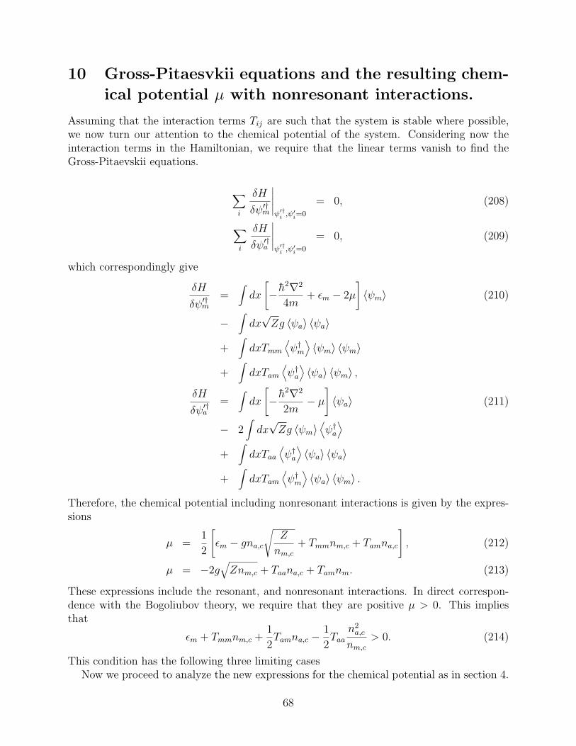
10 Gross-Pitaesvkii equations and the resulting chem-

ical potential µ with nonresonant interactions.

Assuming that the interaction terms Tij are such that the system is stable where possible,we now turn our attention to the chemical potential of the system. Considering now theinteraction terms in the Hamiltonian, we require that the linear terms vanish to find theGross-Pitaevskii equations.

∑i

δH

δψ′†m

∣∣∣∣∣ψ′†

i ,ψ′i=0

= 0, (208)

∑i

δH

δψ′†a

∣∣∣∣∣ψ′†

i ,ψ′i=0

= 0, (209)

which correspondingly give

δH

δψ′†m=

∫dx

[− h

2∇2

4m+ εm − 2µ

]〈ψm〉 (210)

−∫dx√Zg 〈ψa〉 〈ψa〉

+∫dxTmm

⟨ψ†m⟩〈ψm〉 〈ψm〉

+∫dxTam

⟨ψ†a⟩〈ψa〉 〈ψm〉 ,

δH

δψ′†a=

∫dx

[− h

2∇2

2m− µ

]〈ψa〉 (211)

− 2∫dx√Zg 〈ψm〉

⟨ψ†a⟩

+∫dxTaa

⟨ψ†a⟩〈ψa〉 〈ψa〉

+∫dxTam

⟨ψ†m⟩〈ψa〉 〈ψm〉 .

Therefore, the chemical potential including nonresonant interactions is given by the expres-sions

µ =1

2

[εm − gna,c

√Z

nm,c+ Tmmnm,c + Tamna,c

], (212)

µ = −2g√Znm,c + Taana,c + Tamnm. (213)

These expressions include the resonant, and nonresonant interactions. In direct correspon-dence with the Bogoliubov theory, we require that they are positive µ > 0. This impliesthat

εm + Tmmnm,c +1

2Tamna,c −

1

2Taa

n2a,c

nm,c> 0. (214)

This condition has the following three limiting casesNow we proceed to analyze the new expressions for the chemical potential as in section 4.

68

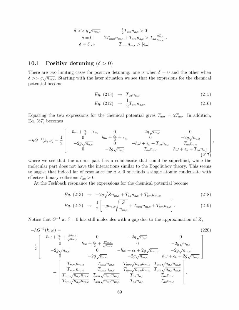
δ >> g√nm,c

12Tamna,c > 0

δ = 0 2Tmmnm,c + Tamna,c > Taan2

a,c

nm,c

δ = δcrit Tmmnm,c > |εm|.

10.1 Positive detuning (δ > 0)

There are two limiting cases for positive detuning: one is when δ = 0 and the other whenδ >> g

√nm,c. Starting with the later situation we see that the expresions for the chemical

potential become

Eq. (213) → Taana,c, (215)

Eq. (212) → 1

2Tamna,c. (216)

Equating the two expressions for the chemical potential gives Tam = 2Taa. In addition,Eq. (87) becomes

−hG−1(k, ω) =1

2

−hω + εk

2+ εm 0 −2g

√na,c 0

0 hω + εk2

+ εm 0 −2g√na,c

−2g√na,c 0 −hω + εk + Taana,c Taana,c

0 −2g√na,c Taana,c hω + εk + Taana,c

,(217)

where we see that the atomic part has a condensate that could be superfluid, while themolecular part does not have the interactions similar to the Bogoliubov theory. This seemsto sugest that indeed far of resonance for a < 0 one finds a single atomic condensate witheffective binary collisions Taa > 0.

At the Feshbach resonance the expressions for the chemical potential become

Eq. (213) → −2g√Znm,c + Taana,c + Tamnm,c, (218)

Eq. (212) → 1

2

[−gna,c

√Z

nm,c+ Tmmnm,c + Tamna,c

]. (219)

Notice that G−1 at δ = 0 has still molecules with a gap due to the approximation of Z,

−hG−1(k, ω) = (220)

12

−hω + εk

2+ gna,c√

nm,c0 −2g

√na,c 0

0 hω + εk2

+ gna,c√nm,c

0 −2g√na,c

−2g√na,c 0 −hω + εk + 2g

√nm.c −2g

√nm,c

0 −2g√na,c −2g

√nm,c hω + εk + 2g

√nm,c

+

Tmmnm,c Tmmnm,c Tam

√na,cnm,c Tam

√na,cnm,c

Tmmnm,c Tmmnm,c Tam√na,cnm,c Tam

√na,cnm,c

Tam√na,cnm,c Tam

√na,cnm,c Taana,c Taana,c

Tam√na,cnm,c Tam

√na,cnm,c Taana,c Taana,c

.

69

Moreover, the gap is produced by the resonant interaction that couples the two channels,which that is still present. Nevertheless, the nonresonant part has the structure of theBogoliubov theory in both the atomic and the molecular part.

10.2 Negative detuning (δ < 0)

Again the chemical potential should be analyzed at the two limiting cases of the detuning,δ = 0 and δ = δcrit. Starting with the case δ = 0 we find that the expressions for the chemicalpotential obey

Eq. (213) → Taana,c + Tamnm,c, (221)

Eq. (212) → 1

2[Tamna,c + Tmmnm,c] . (222)

After substituting these expressions for µ into the inverse Green’s function it becomes

−hG−1(k, ω) = (223)

12

−hω + εk

2+ Tmmnm,c Tmmnm,c Tam

√na,cnm,c Tam

√na,cnm,c

Tmmnm,c hω + εk2

+ Tmmnm,c Tam√na,cnm,c Tam

√na,cnm,c

Tam√na,cnm,c Tam

√na,cnm,c −hω + εk + Taana,c Taana,c

Tam√na,cnm,c Tam

√na,cnm,c Taana,c hω + εk + Taana,c

.

Therefore, it seems that both the molecular and the atomic parts of G−1 at δ = 0 have astructure similar to that of the Bogoliubov theory, and hence of a stable atomic BEC thatmay be superfluid. Interestingly, the coupling has disappeared at this value of the detuning,because of Z(0) = 0. It would seem that we have an uncoupled atomic condensate and agapless molecular condensate, which we know that is not true because both condensate areresonantly coupled at this value of the detuning. We must insist here that this is probablydue to Z that near the Feshbach resonance should also consider many-body effects.

For δ = δcrit the behavior of the chemical potential is

Eq. (213) → −2g√Znm,c + Tamnm,c, (224)

Eq. (212) → 1

2[εm + Tmmnm,c] . (225)

After making the corresponding substitution into Eq. (87) we see again that both the atomicand the molecular part have the required structure to describe BEC, i.e.,

−hG−1(k, ω) = (226)

12

−hω + εk

2+ Tmmnm,c Tmmnm,c 0 0

Tmmnm,c hω + εk2

+ Tmmnm,c 0 0

0 0 −hω + εk + 2g√Znm,c −2g

√Znm,c

0 0 −2g√Znm,c hω + εk + 2g

√Znm,c

.

Notice that the molecular condensate seem to be gapless. Interestingly, the interactions ofthe atomic part are due to the coupling between channels, i.e., resonant interaction, while

70

in the molecular side to the T-matrix for molecule-molecule scattering, Tmm. In addition,the Hamiltonian decouples into the atomic part and the molecular part at this point, as canbe seen from the absence of elements in the off diagonal 2x2 submatrices. This elementsdisappear due to the atomic densities, na,c → 0 as δ → δcrit. Additionally, notice how Taaand Tam disappears from G−1, even though they were the required stabilizing terms in oureigenvalue analysis of the system. Thus it seems that we efectively have two uncoupledcondensates that do not interact between each other: one of gapless molecuels and one ofatoms.

Looking now at the critical point δcrit more closely a new expression for it is found,

εm(δcrit) = −4g√Z(δcrit)nm,c(δcrit) + (2Tam − Tmm)nm(δcrit). (227)

This value is clearly shifted form the previous εm = 2µ, and hence sets a new condition forthe critical value of the detuning δcrit. It is actually more complicated, because the couplingg is very small, which means that probably the nonresonant interactions dominate the righthand side of the equation. Hence, if 2Tam < Tmm the critical detuning is shifted towards thenegative detuning side, but after a certain value of what would effectively be a subtractionthere is no intersection at all because the right-hand side of Eq. (227) shifts downwards. Ifthe other case takes place, 2Tam > Tmm, the critical value δcrit is shifted towards the positivedetuning, but after a certain limit the right-hand side becomes positive, which results againin no intersection with εm. Hence, even though Tmm was not very important when discussingthe stability of the eigenvalues, it does determine the position of the critical detuning δcrit,and furthermore, whether there is a critical point at all through the ratio 2Tam/Tmm. If wenow take the difference ∆µm between the two limiting cases we find

∆µm = −1

4Tmm + Taa + 2

√2g√Z(δcrit), (228)

which gives the energy difference of the molecules with respect to the Feshbach resonance atthe quantum critical point δcrit.

Thus, to summarize this section we remark that G−1 for large positive detuning showsthe molecular part without the structure for superfluidity, while the atomic part does. Atresonance the molecules become gapless, but both the atomic and the molecular part of G−1

show the interaction terms similar to the Bogoliubov theory. Finally, at the quantum criticalpoint G−1 reduces to the uncoupled atomic and molecular submatrices, where the moleculesseem to be gapless, and both have the required interaction terms to give rise to superfluidity.

71

11 Condensate densities nm,c and na,c with nonresonant

interactions Tij.

In this section we rederived the condensate densities using a similar approach as in section5: we equate the two expressions for the chemical potential with interactions Tii foundin section 9 and solve them for the molecular condensate density nm,c. Unfortunately theresulting expression for the molecular density is too complicated to make any direct sensefrom it. Moreover, since the exact expressions for the Tii are not known, we may not evenplot it to see its behavior. Hence, instead of equating the two expressions for the full chemicalpotential, we equated the ones for each of the four limiting cases we have been studying thusfar. Unlike the previous resonantly interacting case, the condensate density seems to have adiscontinuity at the Feshbach resonance, again caused by the molecular renormalization Z.Nonetheless, we expect the same general behavior as for Tij = 0, and see only a shift in thecondensate densities as the effect of including the nonresonant interaction, Tij 6= 0. Let usstudy each case in more detail.

11.1 Negative detuning (δ < 0)

Starting with δ = δcrit the two expressions for the chemical potential (224) and (225) wereequated and solved for the molecular condensate density. One finds

nm,c =2Tamεm − Tmmεm ∓ 4g(−2gZ +

√Z(4g2Z + 2Tamεm − Tmmεm))

(−2Tam + Tmm)2, (229)

where, bearing in mind the resonant case of section 6, it was assumed that the minus signsolution of the quadratic equation is the physical one. In addition, at zero temperature thisexpression must equal nm,c(δcrit) = 1/2 just as before.

Next, we look at δ = 0. Now the expressions for the chemical potential (221) and (222)were solved to find that the molecular condensate density is given by

nm,c =Tam − 2Taa2Tam − Tmm

na,c. (230)

Using the expressions found by Romans, et al. [9] for the scattering length close at resonance,namely, aam = 32a/3, amm = 4a, and the usual aaa = abg, and the expression for thenonresonant interactions Tij = (4πh2aij)/mij where m is the reduced mass that consideresthe atoms involved in each scattering case. This expression reduces to

nm,c(δ) =1

55

(32− 9

abga(δ)

)na,c(δ). (231)

For a → ∞ it becomes nm,c(0) = 32na,c(0)55

≈ 0.58na,c(0). In addition, if we recalculate themolecular condensate density at resonance but now using that since the calculation are beingdone at zero temperature we still have na,c = 1− 2nm,c, one finds

nm,c =2Taa − Tam

4Taa − 4Tam + Tmm. (232)

72

Clearly, the molecular condensate density at δ = 0 depends exclusively on the nonresonantinteractions in our zero-temperature analysis, and is not a fixed number as in the resonantlyinteracting case. Again using the expressions for the interactions Tij at resonance as beforewe find that at δ = 0 the molecular condensate density becomes

nm,c(δ) =32− 9abg/a(δ)

119− 19abg/a(δ), (233)

which for a→∞ becomes nm,c(0) = 32/119 ≈ 0.2689. Correspondingly, na,c(0) = 55/119 ≈0.4621.

11.2 Positive detuning (δ > 0)

Unfortunately one does not find the same result when doing the calculation with the chemicalpotential at resonance from the positive detuning side. For δ > 0 at resonance one equatesthe expressions (218) and (219). Notice how more terms are present with respect to resonancefor negative detuning due to the nonzero value of Z. The resulting formula for nm,c is ratherlarge. Nevertheless, if one uses again the expressions for the nonresonant interactions Tij atresonance and na,c = 1− 2nm,c before taking the limit of the scattering length a→∞, onefinds that nm,c = 0 when the resonance is approached from the positive detuning side. Thisis clearly a discontinuity with respect to the result found for negative detuning. Presumably,there is an error on the positive detuning side due to the approximative nature of Z. Hence,we would expect that in reality there is no discontinuity in the condensate densities at δ = 0just as before, and that their is indeed a molecular condensate.

On the other hand, the case δ >> g√nm,c is similar to that of δcrit. For δ >> g

√nm,c

we do not equate the two expressions (215) and (216). That is, we do not take nm,c = 0.Instead, we cancel the two diverging terms in Eq. (212) with each other, namely, we takethe resonant µm = 0, before equating equation (212) with equation (213). One finds thatthe molecular condensate density is given by

nm,c =4g(2gZ ∓

√Z(4g2Z − na,c(2Taa − Tam)(2Tam − Tmm))) + na,c(2Taa − Tam)(2Tam − Tmm)

(−2Tam + Tmm)2,

(234)where again it still has to be settled whether which sign of the square root is the physicalone, but we presume it is the (-) sign. Notice how the denominator is the same as in theexpression at δcrit. Hence, the general expression for nm,c probably has the same denominatorterm. In addition, if we replace na,c = 1− 2nm,c before doing the previous calculation thenone finds

nm,c =1

(4Taa − 4Tam + Tmm)2

(8gZ + 8T 2

aa + 4T 2am − TamTmm + 2Taa(−6Tam + Tmm)

∓4g√Z(4g2Z + 8T 2

aa + 4T 2am − TamTmm + 2Taa(−6Tam + Tmm))

). (235)

In our zero temperature analysis the molecular condensate density must almost vanish forlarge positive detuning, nm,c ↓ 0 as δ → ∞. In this respect, it is interesting to notice

73

that in expression (235) both the numerator and the denominator have terms proportionalto T 2

am and T 2aa, but not to T 2

mm. Furthermore, the numerator is linear in Tmm, while thedenominator is quadratic. Hence, it seems that the strength of the molecular interactioncould ensure that the molecular density vanishes for large detuning, since it was found insection 8 that it diverges for δ >> g

√nm,c. Also interesting is the fact that all the terms

in the numerator are quadratic in combinations of Tij, which means that even though theirvalues are negative because of the attractive interaction we can consider just their absolutevalue.

Hence, we have found an expression for the condensate densities that also takes intoaccount nonresonant interactions. Even though they seem to have the same behaviour asthe resonantly interacting case, they show a discontinuity at resonance due to Z. Close toresonance we predict nm,c = (32 − 9abg/a)(na,c/55), which in dimensionless units becomesnm,c(0) = 32/119, and consequently na,c(0) = 55/119.

74

12 Conclusions and Discussion

While looking for the elementary excitations of the system and the inverse of the matrixG−1, the most striking feature found was the appearance of instabilities. This leads to themost general conclusion of this research: we must consider nonresonant interactions to havea stable condensate, just as in the Bogoliubov theory.

Regardless of the system being unstable for negative detuning in the resonantly interact-ing case, we nevertheless learned from this analysis the general behavior of the condensatedensities. Indeed we derived analytic expressions that show that the atomic condensate dis-appears at the quantum critical point, that both the atomic and the molecular condensatesare present at the Feshbach resonance, and that even for positive detuning there is a molec-ular condensate in coexistence with the atomic one. Moreover, we derived the ratio betweencondensates, nm,c(δ) = (32−9abg/a(δ))(na,c(δ)/55), which in our scaled condensate densitiesapproximation becomes nm,c(δ) = (32− 9abg/a(δ))/(119− 19abg/a(δ)).

By expanding the dispersions we found expressions that allowed us to see that indeed thequadratic kinetic term of the atomic dispersion is multiplied by an expression that scales itdown, while the linear kinetic term has the scaled chemical potential as a coefficient. Sincethe chemical potential is negative this introduces the imaginary region in the dispersion.Hence, making the chemical potential positive should get rid of this imaginary unstableregion. Regarding the expansion of the molecular dispersion, we found that the kinetic termis multiplied by an expression that scales it up. We concluded that both for positive andnegative detuning, the expansions around k = 0 do not hold for every value of the detuning.

Regarding the stability we showed and concluded that the system can be stabilized fornegative detuning by the atom-atom interactions and by the atom-molecule interactions.Nevertheless, it is not clear wether is may be stable close to resonance for positive detuning.This is not surprising because there we have attractive nonresonant interactions that shouldlead indeed to the collapse of the condensate and the finite life of the molecules. Far fromresonance we find a stable atomic condensate.

Regarding the finite life time of the molecules and the normalization Z, we concludethat the approximation made for the normalization Z of the molecular wave function doesnot accurately describes what happens close to resonance. Many-body effects should beconsidered in its calculation. Hence, we found discontinuities on the functions that dependon it. We conclude that at resonance the value of Z should not be zero, and it is probablyless than one. Far from resonance Z correctly describes the system as was seen from thecondensate density and the dispersion.

By looking at the quantum critical point, at the Feshbach resonance, and far from res-onance on the positive detuning side we were able to describe the system. Thus, at thequantum critical point we found two uncoupled condensates, one of gapless molecules andanother of atoms, both with interactions that could give rise to superfluidity. Aware of thefact that the atomic condensate disappears at this point and considering that the interactionsin the atomic part are due to the resonant interaction and the molecular condensate density,we presume that this atomic condensate is dependent of the molecular one. At resonance wefound also a condensate of gapless molecules and a condensate of atoms resonantly coupledand with nonresonant interactions. This means that the condensates do not disappear atresonance. Far of resonance we found an action describing an atomic BEC with interactions

75

that could give rise to superfluidity. The molecular part seems to be the free condensedmolecular dispersion, and there is still a coupling between channels. Moreover, we havefound an avoided crossing for positive detuning and given an expression for the resonantcase. We expect it to still be present when the nonresonant interactions are considered, butshifted as a function of detuning due to their effect.

Future work should include finding expressions for the different nonresonant interactionsTij in order to be able to properly analyze the interacting case. In addition, the matrix G−1

should be inverted in order to find condensate density fluctuations and be able to go beyondour current zero temperature approximation. Also, an expression for Z that considers man-body effects should be looked into. These three things will allow us to find the dispersion ofthe elementary excitations and the condensate densities with fluctuations. In addition, thestability for positive detuning should be further studied after more precise expresions for thenonresonant interactions are found, in order to determine if the system may be stable.

76

References

[1] Anglin, J. R. & Ketterle, W. Bose-Einstein Condensation of Atomic Gases Nature 416,211-218 (2002).

[2] Dalfovo, F., Giorgini, S., Pitaevskii, L.P., & Stringari, S. Theory of Bose-Einstein Con-densation in Trapped Gases. Rev. of Mod. Phys. 71, 463-511. (1999)

[3] Inouye, S., et al. Observation of Feshbach Resonances in a Bose-Einstein Condensate.Nature 392, 151-154 (1998)

[4] Sakurai, J.J. Modern Quantum Mechanics, Addison-Wesley Publishing Company, Inc.,U.S.A., 1994.

[5] Pethnick, C.J. & Smith, H. Bose-Einstein Condensation in Dilute Gases, CambridgeUniversity Press, U.K., 2002.

[6] Duine, R. Atom-Molecule Coherence in Bose Gases, ISBN 90-393-3522-2.

[7] Timmermans, E., Tommasini, P., Hussein, M., & Kerman, A. Feshbach Resonances inAtomic Bose-Einstein Condensates. Phys. Rep. 315, 199-230 (1999)

[8] Stoof, H.T.C. Lecture notes: Statistical Field Theory. Universiteit Utrecht (2002-2003).

[9] Romans, M.W.J., Duine, R.A., Sachdev, S., & Stoof, H.T.C. Quantum Phase Transitionin an Atomic Bose Gas with a Feshbach Resonance Phys. Rev. Lett. 93, 020405 (2004)

[10] Duine, R. & Stoof, H.T.C. Microscopic Many-Body Theory of Atomic Bose Gases neara Feshbach Resonance J. Opt. B: Quantum Semiclass. Opt. 5, S212-S218 (2003)

[11] Ryder, L.H. Quantum Field Theory, Cambridge University Press, U.K., 1999.

[12] Radzihovsky, L. & Park, J. Superfluid Transitions in Bosonic Atom-Molecule MixturesNear Feshbach Resonance (cond-mat/0312237).

[13] Kokkelmans, S.J.J.M.F., Shlyapnikov, G.V., & Salomon, C. Degenerate Atom-MoleculeMixture in a Cold Fermi Gas. (cond-mat/0308384).

[14] Kittel, C. & Kroemer, H., Thermal Physics, W.H. Freeman and Company, U.S.A, 1980.

77