Atmospheric Temperature Profiles by Ground-based Infrared ...

Air Force Institute of Technology Air Force Institute of Technology

AFIT Scholar AFIT Scholar

Theses and Dissertations Student Graduate Works

3-2000

Atmospheric Temperature Profiles by Ground-based Infrared Atmospheric Temperature Profiles by Ground-based Infrared

Spectrometer Measurements Spectrometer Measurements

Jon M. Saul

Follow this and additional works at: https://scholar.afit.edu/etd

Part of the Atmospheric Sciences Commons, and the Atomic, Molecular and Optical Physics

Commons

Recommended Citation Recommended Citation Saul, Jon M., "Atmospheric Temperature Profiles by Ground-based Infrared Spectrometer Measurements" (2000). Theses and Dissertations. 4854. https://scholar.afit.edu/etd/4854

This Thesis is brought to you for free and open access by the Student Graduate Works at AFIT Scholar. It has been accepted for inclusion in Theses and Dissertations by an authorized administrator of AFIT Scholar. For more information, please contact [email protected].

https://scholar.afit.edu/

https://scholar.afit.edu/etd

https://scholar.afit.edu/graduate_works

https://scholar.afit.edu/etd?utm_source=scholar.afit.edu%2Fetd%2F4854&utm_medium=PDF&utm_campaign=PDFCoverPages

http://network.bepress.com/hgg/discipline/187?utm_source=scholar.afit.edu%2Fetd%2F4854&utm_medium=PDF&utm_campaign=PDFCoverPages



https://scholar.afit.edu/etd/4854?utm_source=scholar.afit.edu%2Fetd%2F4854&utm_medium=PDF&utm_campaign=PDFCoverPages

mailto:[email protected]

ATMOSPHERIC TEMPERATURE PROFILES BY GROUND-BASED INFRARED

SPECTROMETER MEASUREMENTS

THESIS

Jon M. Saul, First Lieutenant, USAF

AFJT/GM/ENP/OOM-11

DEPARTMENT OF THE AIR FORCE AIR UNIVERSITY

AIR FORCE INSTITUTE OF TECHNOLOGY

Wright-Patterson Air Force Base, Ohio

no

APPROVED FOR PUBLIC RELEASE; DISTRIBUTION UNLIMITED

jssES ($>m&m? %mm®mw A.

AFIT/GM/ENP/OOM-11



THESIS

JON M. SAUL, FIRST LIEUTENANT, USAF

AFIT/GM/ENP/OOM-11

Approved for public release; distribution unlimited

The views expressed in this thesis are those of the author and do not reflect the official

policy or position of the United States Air Force, Department of Defense, or the U. S.

Government.

AFIT/GM/ENP/OOM-11



THESIS

Presented to the Faculty of the Graduate School of Engineering and Management

of the Air Force Institute of Technology

Air University

Air Education and Training Command

in Partial Fulfillment of the Requirements for the

Degree of Master of Science in Meteorology

Jon M. Saul, B.S.

First Lieutenant, USAF

March 2000

Approved for public release; distribution unlimited

in

AFIT/GM/ENP/OOM-11



Jon M. Saul, B.S. First Lieutenant, USAF

Approved:

Glen P. Perram (Chairman)

1toL2. Mark E. Oxley (Membei

&. «M&Z- Devin J. Delia-Rose (Member)

3 M4ROQ date

3/^00 date

3 /Vr~ ^ date

IV

Acknowledgments

I wish to thank Lieutenant Colonel Glen Perram, my advisor, for providing me

with the support and opportunity to conduct this research. His expertise and

encouragement kept me on track and was always uplifting.

Also, I wish to thank Major Darrel Goldenstein for sparking my interest in the

area of remote sensing and providing the background information need for this research.

Captain Roy Calfas, from the Air Force Research Laboratory (AFRL), is greatly

appreciated for supplying the up-to-date versions of the PLEXUS atmospheric software

and his ability to answer technical question about the software.

Jon M. Saul

Table of Contents

Acknowledgments v

List of Figures viii

List of Tables x

Abstract xi

ATMOSPHERIC TEMPERATUPvE PROFILES BY GROUND-BASED INFRARED

SPECTROMETER MEASUREMENT

I. Introduction

1.1 Summary 1 1.2 Statement of Problem 2 1.3 Overview 3

II. Literature Review

2.1 Atmospheric Radiation Theory 4 2.2 Retrieval Approaches 7 2.3 Atmospheric Model

2.3.1 PLEXUS 9 2.3.2 SHARC and MODTRAN Merged (SAMM) 11

2.4 Bomem MR-154 Spectrometer 11

III. Methodology

3.1 Overview 15 3.2 Spectral Region Determination 17 3.3 Calculating Kernel Functions 21 3.4 Calculating Atmospheric Brightness Temperature Functions 23 3.5 Collecting Atmospheric Radiance Measurements 25

3.5.1 Spectrometer Setup 25 3.5.2 Spectrometer Calibration 26 3.5.3 Acquiring Atmospheric Radiometrie Data 26

3.6 Computing Atmospheric Temperature Profiles 27

VI

IV. Results

4.1 Introduction 28 4.2 Spectral Range Determination 28 4.3 Collecting Atmospheric Radiance Measurements 29 4.4 Computing Atmospheric Temperature Profiles

4.4.1 Test Case I: 1 December 1999 31 4.4.1 Test Case II: 8 December 1999 34 4.4.3 Summary 36

V. Conclusions and Recommendations 37

Appendix 1: Brightness Temperature and Transmittance Function Data 39

Appendix 2: IDL Programs and Mathcad Templates 52

Appendix 3: Radiosonde Data 67

Bibliography 68

Vita 69

vn

List of Figures

Figure Page

2.1 Example of graphical radiance output from PLEXUS. 10

2.2 Example of graphical transmittance output from PLEXUS. 10

2.3 BomemMR-154 Basic Components. 13

2.4 Principle of operation of the FTIR spectrometer. 14

3.1 PLEXUS graphical radiance output for 15 January 2000. 19

3.2 PLEXUS graphical radiance output for 15 July 1999. 19

3.3 Ratio of 15 July 1999 and 15 January 2000 radiances. 20

3.4 Ratio of 15 January 2000 and 15 July 1999 Transmissivity 20

3.5 Example of output from best-fit software using values from Table 3.3. 22

3.6 Temperature profile used by PLEXUS for 15 November 1999. 23

3.7 Best-fit brightness temperature function using Table 3.4 data. 25

4.1 Calibrated spectrometer output for 1 December 1999. 30

4.2 Calibrated spectrometer output for 8 December 1999. 30

4.3 Temperature plots for 1 December 1999. 32


4.5 Plot of AB using 1 December 1999 radiosonde data. 33

4.6 Plots of AB(z) for 1 December 1999. 33



4.9 Plot of AB using 8 December 1999 radiosonde data.. 35

Vlll

4.10 Plots of AB(z) for 8 December 1999. 36

A. 1.1 Plot of brightness temperature data points and fitted function. 41

A. 1.2 Residual Plot of fitted brightness temperature function. 41

A. 1.3 Plot of transmittance values and fitted function for 2566 cm"1. 43

A. 1.4 Residual plot of fitted transmittance function for 2566 cm" . 43

A.1.5 Plot of transmittance values and fitted function for 2567 cm"1. 45

A. 1.6 Residual plot of fitted transmittance function for 2567 cm"1. 45

A. 1.7 Plot of transmittance values and fitted function for 2568 cm" . 47


A. 1.9 Plot of transmittance values and fitted function for 2569 cm"1. 49


A. 1.11 Plot of transmittance values and fitted function for 2570 cm" . 51


IX

List of Tables

Table Page

3.1 Highly Variable Atmospheric Constituents and their Absorption Bands. 18

3.2 Pathlengths used in calculation of transmittance. 21

3.3 Examples of transmittance values for specific pathlengths. 22

3.4 Example of temperature and calculated brightness temperatures for 2568 cm"1. 24

4.1 Most promising frequencies. 29

4.2 Atmospheric radiance measurements collected by the spectrometer. 31

A. 1.1 Numeric Summary of fitted brightness temperature function parameters. 40

A. 1.2 Numeric summary for transmittance and kernel parameters for 2566





cm

cm'

cm

1 cm'

cm'

42

44

46

48

50

AFIT/GM/ENP/OOM-11

Abstract

A method to recover atmospheric temperature profiles using a ground-based

Fourier Transform Infrared spectrometer was investigated. The method used a difference

form of the radiative transfer equation, a Bomem MR series Fourier Transform Infrared

Spectrometer to collect atmospheric radiance values, and the Phillips Laboratory Expert-

assisted User Software (PLEXUS) atmospheric radiance model, to recover an

atmospheric temperature profile. The method researched uses radiance values from both

the spectrometer measurements and the atmospheric model, along with kernel functions

calculated by the atmospheric model as input to a difference form of the radiation transfer

equation. From this the change in brightness temperatures was determined. The method

assumes that the actual brightness temperature profile is a summation of a standard or

reference brightness temperature profile plus some change in the brightness temperature.

The brightness temperature profile used by the atmospheric model is the reference

brightness temperature profile. Planck's Law was employed to transform the calculated

brightness temperature function into a temperature function. A temperature profile was

retrieved, although significant differences existed between the recovered temperature

profile and a radiosonde recovered temperature profile.

XI


SPECTROMETER MEASUREMENT

I. Introduction

1.1 Summary

In the last decade, great strides have been made in the area of remote sensing by

surface based equipment. Advances in technology and reduction in the cost associated in

the manufacture of remote sensing equipment have made the plausibility of remote

sensing a reality. In particular, remote sensors are sought for as a means of replacing or

accenting current atmospheric measurement techniques.

Radiosondes are the principle devices used to obtain atmospheric profiles. A

single radiosonde costs approximately $100. Typically, radiosonde sites launch

radiosondes twice a day. Even with these conservative costs, a yearly supply of

radiosondes for one station can cost over $73,000. This estimate does not include the cost

of tracking the radiosonde or disseminating the data. Using surface-based remote sensors,

atmospheric profiles can be recovered (Smith et al. 1990). The infrared spectrometer is

one instrument being studied for its use in obtaining infrared spectral data to produce

atmospheric profiles. Smith et al. (1990) believes a basic interferometer system capable

of performing ground-based atmospheric profiling would cost less than $50,000. A

ground-based infrared spectrometer system offers the possibility of saving millions of

dollars annually.

A problem with the current profiling system, radiosondes, is the temporal

resolution of upper air profiles. Typically, radiosondes are launched twice a day, at 00Z

and 12Z, and recover one atmospheric profile for each radiosonde launched. Because

atmospheric profiles of the troposphere are constantly changing, the recovery of

atmospheric profiles twice a day leaves large temporal gaps in the data. An infrared

spectrometer has the ability to produce atmospheric radiance measurements every few

seconds. From these radiance measurements, a profile can be calculated for each radiance

measurement. An increased temporal resolution provided by ground-based spectrometers

will enhance all areas of meteorology.

With the cost and the temporal coverage benefits, the use of an infrared

spectrometer to supplement or replace the radiosondes as the primary mean of retrieving

atmospheric profiles looks promising. The remaining question is which process to use to

recover atmospheric profiles.

1.2 Statement of Problem

This research used a difference form of the radiative transfer equation, a Bomem

MR series Fourier Transform Infrared Spectrometer (FTIR) to collect atmospheric

radiance values, and the Phillips Laboratory Expert-assisted User Software (PLEXUS)

atmospheric radiance model, to recover an atmospheric temperature profile. The method

researched uses radiance values from spectrometer measurements and the atmospheric

model, along with transmissivity value calculated by the atmospheric model as input to

the difference form of the radiation transfer equation. From this the change in brightness

temperatures can be determined. The method assumes that the actual brightness

temperature profile is a summation of a standard or reference brightness temperature

profile plus some change in the brightness temperature. The brightness temperature

profile used by the atmospheric model is the reference brightness temperature profile.

The goal is to determine the changes in the atmospheric brightness temperature profile

and to recover the actual brightness temperature profile. The temperature profile can be

calculated using the relationship between brightness temperature and temperature in

Planck's Law.

1.3 Overview

This thesis consists of five chapters. Chapter II contains literature review

material, which contains fundamental material to support this research. Chapter III

describes the procedures used during this research. Chapter IV presents the results of this

research. Chapter V discuses conclusions made from this research.

II. Literature Review

2.1 Atmospheric Radiation Theory

The concept of using radiative transfer to formulate the absorbing, scattering, and

creation of natural radiation within a volume filled with particles interacting with

radiation was developed for astrophysical problems (Schanda, 1986). Radiation can be

absorbed by atmospheric gases in continuum: (ionization and photo-dissociation), and

discrete (electronic transitions, vibrational transitions, and rotational transitions) bands.

In the infrared region, vibrational and rotational transitions account for most of spectral

line emissions (Goody and Young, 1989). Transitions between two energy levels produce

. discrete spectral line emission or absorption, but due to molecule collision, spectral

broadening occurs and distorts a molecule's energy levels. This distortion in the energy

level causes the transitions to occur over a range of frequencies instead of one discrete

frequency.

The radiative transfer equation (RTE) accounts for all four possible radiative

interactions: the emission of radiation by a gas, the absorption of radiation by a gas, the

scattering of radiation out of a beam, and the scattering of radiation into a beam. A

general formula for the instantaneous change of the radiance is:

— =A+B+C+D (2.1)

where,

9 1 L = monochromatic radiance (W/cm cm" sr)

s= distance along a beam (meters)

A = absorption of radiation by a gas (W/cm2 cm"1 m"1)

B = emission of radiation by a gas (W/cm cm" m")

? 1 1 C = scattering of radiation out of a beam (W/cm cm" m")

D = scattering of radiation into a beam (W/cm2 cm"1 m"1)

A special case of the RTE is sometimes referred to as the Schwarzchild's

equation. The Schwarzchild equation assumes no scattering of radiation into or out of the

beam. On a clear, cloudless day the Schwarzchild's equation (Wallace, 1997), Equation

2.2, is valid for the atmosphere, and is:

CO

LÄ^ + \BÄ(z)WÄ{z,v)dz (2.2) 0

where,

9 1 L0 = spectral radiance at the top of the atmosphere (W/cm cm" sr)

9 1 Lx = spectral radiance received (W/cm cm" sr)

ju = cos(6)

6 = zenith angle

BÄ (z) = blackbody radiance (W/cm cm")

WA(z,/i) = kernel function (change of transmittance with respect to height)

z = height (meters)

A. = wavelength (meters)

Retrieval approaches use an inverse form of the radiative transfer equation to

solve for atmospheric temperature profiles. Using the Schwarzchild's form of the

radiative transfer, Equation (2.2), and calibrated radiance values obtained from an

infrared spectrometer, it is possible to calculate a temperature profile. This version of the

radiative transfer equation assumes no scattered or diffuse radiation. These assumptions

are viable for the infrared spectrum in the atmosphere in the absence of clouds (Kidder

and Vonder Haar, 1995).

A linear approximation for the radiative transfer equation in a matrix form is

(Schanda, 1986):

lx = WABA (2.3)

where,

L, = vector of monochromatic radiance values (W/cm2 cm"1 sr)

WA = a matrix of change in transmittance values

-* 9 1 BA = vector of brightness temperatures (W/cm cm")

Using the ground-based spectrometer, the measured radiance, Lx, is observed and

the weighting functions, WA(z,//), can be calculated using an atmospheric model. An

inverse method uses the observed radiances to calculate a Planck's radiance profile. The

inverse of the non-scattering radiative transfer equation is:

W;%=BX (2.4)

With Bx known, then temperature is calculated using Planck's function.

BA =C,/l"5/[exp(C2/ir)-l]

(2.5)

where,

9 1 B^ = brightness temperature (W/cm cm")

T = temperature (Kelvin)

% = wavelength (meters)

Ci= 1.1919439 xlO"16Wm2

C2= 1.438769 xlO"2mK

2.2 Retrieval Approaches

In late 1988, researchers conducted the Ground-based Atmospheric Profiling

Experiment (GAPEX) (Smith et al, 1990). One part of GAPEX involved using a high-

resolution interferometer (HIS) to measure the infrared spectrum. Atmospheric

temperature and water vapor profiles were calculated using the measured radiances from

the HIS. Researchers used the inverse of the non-scattering radiative transfer matrix,

Equation 2.4, to recover temperature profiles. The HIS was used to obtain atmospheric

radiance data and statistical data was used to determine the kernel function.

In mid 1992, researchers experimented with retrieving atmospheric profiles from

radiance values obtained by a Double Beam Interferometer Sounder (DBIS) (Therlault

1993); (Therlault et al, 1996). The DBIS experiment used the approach based on the

minimum information method. There are two main advantages to this approach: one,

"first-guess" profiles are not required, and second, simultaneous retrieval for multiple

parameters is possible.

The method works as follows: first, researchers assumed that the measured

radiance is a function of the actual radiance plus a linear perturbation (Therlault 1993);

(Therlault et al, 1996). The perturbations are linearized about a point Lo,

L(v) = L0(v) + dL(v) (2.6)

where L(v) is the measured spectral radiance, Lo(v) is the actual radiance, and dL(v) is

the perturbation of the radiance. Second, the approach employs a linear difference

technique in a matrix form.

BJt=[W,S-elW + S-bTW'S;lLJl (2.7)

This approach constrains the solution by weighting the equation with two error matrices,

Se and Sb- The error weighting matrices accounts for instrument error and uncertainty in

the "first-guess" profile.

Obtaining the damping matrix, Sb, poses a problem (Theriault 1993:); (Theriault

et al, 1996). The selection of the damping matrix must be completed empirically.

Another problem deals with the time required to iterate to a solution.

In another experiment, researchers at the University of Wisconsin-Madison use

the Atmospheric Emitted Radiance Interferometer (AERI) to measure atmospheric

radiance every ten minutes. Atmospheric temperature profiles were produced using the

measured radiance. AERI uses an inverse technique to retrieve a temperature profile

from ground-based radiance measurements. Using the inverse of the radiative transfer

equation, researchers at the University of Wisconsin-Madison use a statistical first guess

of an atmospheric temperature profile and the measured radiances to solve the inverse

radiative transfer equation. The University of Wisconsin-Madison has detailed

information on the AERI project at http://cimss.ssec.wisc.edu/aerlwww/aeri/.

Häuser (1999) experimented with the Bomem MR-154 FTIR spectrometer to recover

infrared radiance measurements of the atmosphere. The retrieval method used a least

squares solution to obtain a temperature profiles from observed radiances. The method

involves multiplying both sides of equation 2.2 by the transpose of the weighting

function, which Häuser identifies as the "kernel", and solving for blackbody

temperatures. The weighting functions or kernels, W, are the changes in monochromatic

transmissivity over path length. MODTRAN calculations are used to compute the

weighting functions. Once the weighting function was determined, the inverse matrix

was solved.

In his results, Häuser (1999) states that the procedure did not work, but gives no

explanation as to why.

2.3 Atmospheric Models

2.3.1 PLEXUS

PLEXUS is a user-oriented software platform, which integrates user input into

DOD standard atmospheric and celestial models. PLEXUS provides a graphical interface

for the following Air Force Research Lab (AFRL) codes: MODTRAN3.7, SAMM1,

FASCODE3P, and SAG1. The PLEXUS software allows the user to input parameters,

then the PLEXUS software converts the numeric input to the native units of the

applicable AFRL code. The source codes of the models are not altered in any way.

PLEXUS is available on a CD through AFRL (PLEXUS, 1999).

CN

0) ü c

T3

cr

o Q.

CO

0.0001

1e-5

1e-6

1e-7

1e-8

is 1e-9

= =3 r= 1 —= = , 1 j

1 i ]

.=31 I 1 «jmj=d == =

irw,

=_L_J j "

-T- s V.

650750850950 1150 1350 1550 1750 1950 2150 2350 2550 2750 2950

Frequency (cm-1)

Figure 2.1 Example of graphical radiance output from PLEXUS.

Ü c TO

C

L_

Ü <D Q.

CO

0.8

0.6

0.4'

0.2'

0

650750850950 1150 1350 1550 1750 1950 2150 2350 2550 2750 2950

Frequency (cm-1)

Figure 2.2 Example of graphical transmittance output from PLEXUS.

10

2.3.2 SHARC and MODTRAN Merged (SAMM)

The SAMM model was used to calculate all model derived transmittance and

radiance data. SAMM is an atmospheric model, which combines the Moderate

Resolution Transmittance Model (MODTRAN) and the Strategic High-Altitude

Atmospheric Radiance Code (SHARC). MODTRAN was developed by the Air Force

Research Laboratory as a way to calculate path radiance and path transmittance in the

infrared, visible, and near ultraviolet spectral regions for a given atmospheric path below

100 km. MODTRAN is a band model that uses empirically derived data to compute

transmittance and radiance values. SHARC3 is a non-Local Thermodynamic Equilibrium

(NLTE) code for computing infrared path radiance for arbitrary paths between 50 and

300 km in the 2 - 40 micron spectral region. It also incorporates SHARC Atmospheric

Generator (SAG). SAG is an AFRL code that calculates atmospheric profiles based on

geophysical and geographical information. SAG uses the NRL climatological database

(PLEXUS, 1999), which is comprised of atmospheric profiles of mean monthly

concentrations at 1 to 5 km increments and ten-degree latitude increments. SAG

interpolates between these values and PLEXUS uses the output for SAMM.

2.4 Bomem MR-154 Spectrometer

The Bomem MR-154 Fourier Transform Infrared (FTIR) Spectoradiometer is an

instrument capable of obtaining highly accurate spectral features of a target source in the

525 cm"1 to 6000 cm"1 (19 urn to 5.55 urn) range with a maximum resolution of 1 cm" .

The MR-154 FTIR spectrometer is comprised of two subsystems: the data processing

and control assembly and a Michelson interferometer.

11

The data processing and control system consists of a personal computer, which

runs the Research Acquire software package. The software package provides a user

interface to control the interferometer to collect data. The software also allows a user to

process the data to produce calibrated radiance files.

Figure 2.3 is a top view of the interferometer with the main components

identified. The main components consist of two detectors, a collimator with an aperture,

transfer optics with apertures and a cold subtraction source. The interferometer's two

detectors are the mercury, cadmium, and telluride, MCT, a solid-state detector and the

indium antimonide, InSb, a solid-state detector. The MCT detector allows for the

collection of radiometric data in the 525 cm"1 to 1800 cm"1 (19 |am to 5.55 (im) region.

The InSb detector allows for the collection of radiometic data in the 1800 cm"1 to 6000

cm"1 (5.56 urn to 1.67 |um) region. The cold subtraction source and the detectors are filled

with liquid nitrogen to reduce the thermal noise of the instrument. The collimator and

transfer optics, along with their apertures, control the radiometric data reaching the

detectors.

Figure 2.4 is reproduced from Häuser (1999). It displays the principle of operation

of the FTIR spectrometer. Source radiation enters the spectrometer through the input

collimator (1). Then radiation is split by a beam splitter, with one beam reflected by a

stationary mirror while, the other's path length is varied with a moving mirror (Dl). Then

the radiation beam is recombined (2) and recorded as an interferogram.(3) A Fourier

transform is applied to the interferogram to produce a raw spectrum (4). The raw

spectrum is calibrated using a previously determined calibration spectrum (5). The final

output is calibrated spectral data (6). Further information on the components of the

12

Bomem MR-154 FTIR Spectoradiometer and its operation can be found in the Bomem

MR Series Documentation set (BOMEM Inc. 1997).

Aperture

Collimator

Connectors and resolution selector

Transfer optics and aperture Cold subtraction source

Figure 2.3 Bomen MR-154 Basic Components.

13

Top View of Internal Components

I Cube Comer

Cube Comer

Incident Beam

<■

Beamsplitter

\K Recombined Beam

Input Collimator Source

\ Aperture Wheel

Recombined Calibrated Spectral

Fourier Transform Applied

30CO 3500

Calibration

Figure 2.4. Principle of operation of the FTIR spectrometer. Incident energy, 1, aperture and encounters beam splitter at point 2. The beam is recombined where and destructive interference result represented by the interferogram at 3. A Fourier is applied to the interferogram and a raw spectrum results. At 5, a calibration completed. Finally, a calibrated spectral plot is obtained at point 6 (after BOMEM Users Manual.) (Häuser, 1999).

14

III. Methodology

3.1 Overview

This chapter presents the methodology used during the research. Starting with

Equation 2.2, Schwarzchild's equation for the actual radiance is:

L,^\w,{Z)B,{z)dz (3.1)

where,

L = Monochromatic radiation for a specific wavelength of the atmosphere

(W/cm2 cm"1 sr"1)

Wx(z) = Kernel function for a specific wavelength of the atmosphere

B^z) = Brightness temperature function for a specific wavelength of the atmosphere (W/cm2 cm"1)

z = height (meters)

A second radiation equation is employed as a reference:

4 = fazßS&h (3.2)

where,

Zj = Monochromatic radiation for a specific wavelength from an atmospheric model (W/cm2 cm"1 sr"1)

W2(z) = Kernel function for a specific wavelength from an atmospheric model

Bjiz) = Brightness temperature function for a specific wavelength from an atmospheric model (W/cm cm")

Subtracting Equation 3.2 from Equation 3.1 provides a relationship between the

atmospheric model derived parameters and the atmospheric parameters.

15

2, -4 = j" W{z\Btf)dz- J W:z)24(z)Jz (3.3)

Assuming

B[(z)=B2(z)+m.z) (3-4)

9 1 using A8(z) =Change in brightness temperature function (W/cm cm") then:

2, ~4 = J W(z\(B2(z)+AB(z))dz- J B£(z)*^(z>fe (3.5)

Expanding terms and rearranging,

k-h = \ Wl(z)B1(z)dz+ J W(z\Wz)dz- J 0{z)2*Bz(z)dz (3.6)

/,-^-J ^(z)^(z)Jz+ J W(z\ *B2(z)dz= j" ^(z), A5(z>fe (3.7)

If the kernel functions, W(z), that do not change with time can be found, that is

W,(z) = W2(z) then,

Z,-L, = jV(z)A5(z>fe (3.8)

In this research, W, L2 and B2 are determined using PLEXUS and its integrated

atmospheric model, SAMM1. Li is actual radiometric measurements using the Bomem

MR-154 spectrometer.

We construct an algorithm to find the temperature from the radiometric

measurements.

Step 1. We first search regions of the spectrum where the kernel functions are insensitive

to the state of the atmosphere while there is a significant change in the observed radiance

(see Section 3.2).

16

Step 2. Kernel functions are calculated using the PLEXUS atmospheric model. The

kernel functions will be determined by calculating the transmittance at a number of

specified altitudes and then determining the path derivatives dx/dz (see Section 3.3).

Ideally, the kernel functions should be continuous, because the change in

transmittance is continuous in the atmosphere. The kernel functions calculated with

PLEXUS are discrete. For this reason, continuous functions are fitted to the discrete

kernel values (see Sections 3.3 and 3.4)..

PLEXUS uses predetermined atmospheric profiles to calculate radiance outputs.

Kernel functions were tested by comparing a recovered temperature profile, using the

PLEXUS radiance output and previously determined kernel functions, to the model input

temperature profile.

Step 3. The final step is to use the spectrometer to recover actual radiance measurements

of the atmosphere and determine the temperature profile using the calculated kernel

functions. This resulting temperature profile will be compare to a local radiosonde-

recovered temperature profile coincident in time (see Sections 3.5 and 3.6)..

3.2 Spectral Region Determination

Spectral regions from 500 cm"1 to 3000 cm"1 were chosen based on the Bomem

spectrometer's spectral range. To minimize the number of possible wavelengths, regions

of the spectrum were disqualified as being poor choices for recovering temperature

profiles. The first was to disqualify all regions whose absorption is mainly due to highly

variable density profiles of atmospheric constituents. Goody and Yung (1989) list three

constituents as variable or highly variable and give the appropriate absorption bands

associated with the constituents. Table 3.1 lists these constituents and their absorption

17

bands. These absorption bands were disqualified. Disqualifying these absorption bands

leaves the band from 2400 cm"1 to 2800 cm"1.

Table 3.1 Highly Variable Atmospheric Constituents and their Absorption Bands.

Constituent Absorption Band Transition

H20, water 0-1000 cm-1 rotational

H20, water 900 ~ 2400 cm-1 vibrational

H20, water 2800 ~ 4400 cm-1 vibrational

03, ozone 1000-1100 cm-1 vibrational

CO, carbon monoxide 2100-2400 cm-1 vibrational

Two dates were chosen based on the National Research Laboratory, NRL, data

base temperature profiles. These temperature profiles were used as the inputs to

PLEXUS. The months of January and July were chosen based on the greatest differences

in the temperature profiles. PLEXUS software was used to calculate radiance value for

650 cm"1 to 3000 cm"1. Figure 3.1 is the PLEXUS derived January radiance profile, while

Figure 3.2 is the PLEXUS derived July radiance profile. The values are calculated for a

path length of infinity, the total atmosphere. Figure 3.3 is the ratio of the two PLEXUS

derived radiance profiles.

Transmittance values were calculated using PLEXUS over the 650 cm"1 to 3000

cm"1 range for both January and July. At each discrete height, the quotients of the July

and January transmittance values were determined. Wavenumbers where the quotients

were one or near one and there was a significant change in the radiance were considered

to be caused by mostly temperature changes in the input atmospheric profiles. Figure 3.4

displays the ratio of the January and July transmittance values calculated for a path length

of the entire atmosphere.

(M

o CD a.

0.0001

1e-5

1e-6

1e-7

1e-B

1e-9

le-10

= ==4=^^^ ======= —!—|—i—r _=4 i i . J \ -U ==raW X* ill p4--==i =±s

i i i —\-^ ^ "•---I-,.

-—\—I—- —i—

! I : ! 1 i

'1 .f-T

1 i 1

i | —1—i—

1 ! 750 950 1150 1350 1550 1750 1950 2150 2350 2550 2750 2950

Frequency (cm-1)

Figure 3.1 PLEXUS graphical radiance output for 15 January 2000.

p 0.0001

E ü

le-5 IS)

CN b ü 1e-6 ^

£ 1fi-7 CD U c

le-8 (B

QL

~m 1e-9 t_ •*-> c u t CD Q.

CO

I 1 ——

-IJSÜ =3 J- I

-t^ H" V

650750850950 1150 1350 1550 1750 1950 2150 2350 2550 2750 2950

Frequency (cm-1)

Figure 3.2 PLEXUS graphical radiance output for 15 July 1999.

19

03 a:

500 1000 1500 2000 Wavenumber (cm-1)

2500 3000

Figure 3.3 Ratio of 15 July 1999 and 15 January 2000 radiances.

1.25

1-

O 0.75- g

0.54

0.25

650 1120 1590 2060 2530 3000

Frequency (cm-1)

Figure 3.4 Ratio of 15 January 2000 and 15 July 1999 transmissivity.

20

3.3 Calculating Kernel Functions

PLEXUS was used, in a batch mode, see Appendix 2, to calculate transmittance

values over the 650 cm"1 to 3000 cm"1 range with varying pathlengths. The following

pathlengths were used, see Table 3.2..

Table 3.2 Pathlengths used in calculation of transmittance.

Lower Height Upper Height Change in Pathlength

0 meters 2 kilometers 10 meters

2 kilometers 10 kilometers 50 meters

10 kilometers 50 kilometers 1000 meters

50 Kilometers 300 kilometers 5000 meters

For selected wavenumbers, the following equation form, Equation 3.9, was

calculated by a best-fit software package to fit a function to the discrete transmittance

values.

The equation form, Equation 3.10, was used for all calculated transmittance

functions, x(z) as a function of height, z.

<z) = a+cz

l+bz+dz2 (3.9)

Next, the derivative of transmittance with respect to height, that is, the kernel

function, was determined. Equation 3.14 shows the derivative of x(z) and was used for all

used for all calculated kernel functions, W.

W(z)=dz(z)/dz=- -{-c+cdi +ab+2ad$

(l+bz+dz2)1 (3.10)

The parameters for the transmittance and kernel functions calculated can be found in

Appendix 1.

21

The following is an example of the method used to determine the kernel

functions. Table 3.3 is an example of transmittance values at given heights. Figure 3.5 is

the output from the best-fit software using data from Table 3.3.

Table 3.3 Example of transmittance values for specific pathlengths.

Path Length (m) Transmittance 0 1.000000 100 0.816010 200 0.714550 300 0.642030 400 0.584930 500 0.538240 600 0.499040 700 0.465520 800 0.436640 900 0.411210 1000 0.389160

■u

1.1

1

0.9

0.8

E 0.7

re 0.6

0.5

0.4

0.3

y=(a+cx)/(1+bx+dx2)

a=0.99832304 0=0.0084152028 c=0.0057232514 d=7.8675985e-06

0 250 500 750 10 00 12! Height (m)

Figure 3.5. Example of output from best-fit software using values from Table 3.3.

22

3.4 Calculating Atmospheric Brightness Temperature Functions

Atmospheric brightness temperatures were calculated using Planck's formula and

physical temperature provided by the atmospheric model. Temperatures from the

PLEXUS software were given at discrete height values, see Figure 3.6.

L_ =3

-t—«

CCS L_ <D CL E

3UU

290J

280-

270-

260-

250-

240-

230-

220-

210-

900

—V- * i t I !

V { | j [■/■■ I ~N^j

1 j j j j

20000 40000 Height (m)

60000

Figure 3.6 Temperature profile used by PLEXUS for 15 November 1999.

These temperature values were used to calculate the brightness temperature at

specific wavelengths using Planck's law.

Bx =C,Ä"/[exp(C2/ÄT)-l]

where,

9 1 Bx = brightness temperature (W/cm cm")

T = temperature (Kelvin)

(3.11)

23

X = wavelength (meters)

Ci= 1.1919439 xlO"16Wm2

C2 = 1.438769 xl0"2m

Once the discrete brightness temperature profile is determined, a best-fit software is used

to fit a function to the data. The brightness temperature function calculated for this

research can be found in Appendix 1.

The following is an example of the method used to determine the brightness

temperature functions. Table 3.4 is an example of calculated brightness temperature at

given heights and temperatures using a wavelength of 2568 cm"1. Figure 3.7 is the output

from the best-fit software using data from Table 3.4.

Table 3.4 Example of temperature and calculated brightness temperatures for 2568 cm" .

9 1 Brightness Temperature (W/cm cm") 3.91E-07 3.38E-07 2.68E-07 1.98E-07 1.39E-07 9.34E-08 6.12E-08 3.96E-08 2.57E-08 1.70E-08 1.16E-08 8.27E-09 6.20E-09 4.89E-09 4.07E-09 3.58E-09 3.34E-09 3.26E-09 3.29E-09 3.39E-09 3.53E-09

Height (m) Temperature 0 290.2

1000 286.9 2000 281.9 3000 275.6 4000 268.4 5000 260.9 6000 253.4 7000 246.0 8000 239.2 9000 232.9 10000 227.4 11000 222.8 12000 219.0 13000 216.0 14000 213.7 15000 212.1 16000 211.3 17000 211.0 18000 211.1 19000 211.4 20000 211.9

24

4.5e-07

y=(a+cx+eS+gx3+ix*+k>?)/(1 +bx+d>?+fx3+hx^+j>^)

a=3.9076456e-07 b=-0.00020002041 c=-1.1778633e-10 d=5.958575e-08 e=1.5860199e-14 fc-8.3255991 e-12 g=-1.1397826e-18 h=7.9985016e-16

i=4.3060194e-23 j=-2.7438458e-20 k=-6.7821101 e-28

E (> 4e-07 r\i

F 3.5e-07 o 5 3e-07 <x> Z5 2.5e-07 m k_

<x> n 2e-07 E I- 1.5e-07 LD CO 1e-07 T

4—'

O) 5e-08 ÜÜ

\ i I ! i V i i

\ Y : V ; •

\i I I i

i r~*~- ■ ■ ■ ■ t ' ' ■ ■ 5000 10000 15000

Height (m) 20000 25000

Figure 3.7 Best-fit brightness temperature function using Table 3.4 data.

3.5 Collecting Atmospheric Radiance Measurements

The MR-154 spectrometer was used to obtain atmospheric radiance

measurements. The following sections details the setup of the equipment, equipment

calibrations and the recovering of atmospheric radiance values.

3.5.1 Spectrometer Setup

The setup of the MR-154 spectrometer was conducted following the procedures in

the Bomem MR Series Documentation Set (1997). The MR-154 spectrometer's was

deployed on the rooftop of Bldg 640 at Wright-Patterson AFB. The spectrometer's tripod

was set up and leveled using the bubble-level located on the tripod. Once the tripod was

leveled the azimuth was calibrated using a compass. Next the main assembly was

attached to the tripod and the cold subtraction source and detectors were attached to the

25

main assembly. The cold subtraction source and detectors were filled with liquid

nitrogen to ensure a minimal thermal noise. The collimator, amplifier and resolution

settings were set to the best setting determined by Häuser (1999): the gain was full, the

aperture was at diameter of 6.4 mm, and the resolution was 1 cm"1. The cover to the main

assembly was attached and the level of the main assembly was rechecked. The main

assembly's internal heater was set to 30 C and allowed to reach equilibrium. Finally the

optics, a narrow view telescope, was attached to the main assemble. The narrow view

telescope is a Cassegrainian telescope with a focal length of 12 cm. It has a narrow field

of view of only 5 milliradians or 0.286 degrees. Cabling was connected from the

spectrometer to the computer. This completes the set up of the spectrometer.

3.5.2 Spectrometer Calibration

Spectrum calibration was conducted following the procedures in the Bomem MR

Series Documentation Set (1997). A blackbody was place in front of the spectrometer's

collimator ensuring it filled the equipment's field of view. This essentially eliminated any

stray radiance. The blackbody was set to four different temperatures: 0C, IOC, 30C and

50C, and allowed to stabilize at each temperature. Once the black body stabilized, at each

temperature, a radiometric reference was obtained. After the radiometric references were

obtained, a calibration file was calculated using the Compute Radiance Correction

function in the Research Acquire software. This completes the calibration requirements.

3.5.3 Acquiring Atmospheric Radiometric Data

After the setup and calibration of the equipment, acquiring radiometric data is

obtained easily. At a selected time, an interferogram is obtained using the spectrometer.

A interferogram measurement was comprised the average of 50 scans. After the

26

interferogram is obtained, no further use of the spectrometer is needed. The Research

Acquire software constructs radiance file from the interferogram, then the calibrated

reference file is use to calibrate the radiance file. At this point, calibrated radiance

measurements can be taken from the output files or from the display screen.

3.6 Computing Atmospheric Temperature Profiles

The key to this method is to determine AB (z), the change in brightness

temperatures as a function of height. Once AB (z) is determined it is used to calculate the

actual brightness temperatures by following the previous assumption that the actual

brightness temperatures are a summation of the brightness temperature used in PLEXUS

and a change in the brightness temperature, B(z)actuai = B(z)pieXUs + AB(z), where BactUai is

the physical brightness temperature and BpieXus is the brightness temperature used by

PLEXUS software. Temperature is calculated from Bactuai using Planck's Law.

The first step is to calculate the coefficients for AB(z). This is accomplished by

using^ -4 =\w(z)AB(z)dz, see Equation 3.8. W(z) is calculated using PLEXUS derived

kernel functions. The change in radiance, (Z,--^)» is calculated using spectrometer

radiance measurements, Z, and PLEXUS radiance calculations, L,.

The Mathcad templates, calc_profile_2.mcd and calc_profile_3.mcd, see

Appendix 2, are used to retrieve the new temperature profiles. Template

calc_profile_2.mcd assumed AB(z)=a+bz and template calc_profile_2.mcd assumed

AB(z)=a+bz+cz2.

27

IV. Results

4.1 Introduction

This chapter lists the results observed during the research and the analysis on

success of the physical retrieval method employed. First, the results of spectral range

determination are presented. Next, the results from the collection of radiometric data are

presented. Finally, the results of the method used to recover atmospheric temperature

profiles are discussed.

4.2 Spectral Range Determination

Table 4.1 lists the wavenumbers meeting the selection criteria presented in

Chapter 3. First, radiance values for frequencies influenced by highly variable

atmospheric constituents were eliminated. This disqualified a significant portion of the

initial 650 cm"1 to 3000cm"1 region, hence wavenumbers outside of the 2400 cm"1 and

2800 cm"1 region were disqualified. Secondly, the maximum change between the July and

January transmittance values at all levels was required to be less than five percent. Next,

there was to be a significant change between the January and July radiance values. Figure

3.3 was used to subjectively eliminate the region between 2400 cm"1 and 2500 cm" .

Finally, kernel functions not equal to zero above 50,000 meters were eliminated. This

was done to decrease the require integration of the radiative transfer equation from 0 km

- 300 km to 0 km - 50 km.

Of frequencies listed in Table 4.1, a final set of wavenumbers, 2566 cm"1 to 2570

cm"1, was chosen because they are the largest set of continuous wavenumbers meeting the

criteria. The larger set allows the use of five independent pieces of information, thereby

28

allowing a choice in the assumed change in brightness temperature function, AB(z), to

have up to five coefficients.

Table 4.1 Most promising frequencies.

Wavenumber (cm-1)

Ratio of January and

July Transmissivity

values

Height where transmissivity change with Height = 0

(km)

Change in Radiance with

height = 0 (km)

Change in Radiance

Between July and 2 January (W/cm

srcm ) 2534 0.96038 50 50 4.1655E-09 2535 0.97145 50 50 3.3583E-09 2536 0.97491 50 50 3.2157E-09 2537 0.97728 50 50 3.0976E-09 2538 0.97460 50 50 3.2201E-09 2539 0.96863 50 50 3.7177E-09 2540 0.97797 50 50 3.0406E-09 2541 0.97816 50 50 3.0577E-09 2542 0.97875 50 50 3.0566E-09 2566 0.97699 50 50 2.5064E-09 2567 0.97666 50 50 3.2534E-09 2568 0.97922 50 50 2.7339E-09 2569 0.97636 50 50 2.9552E-09 2570 0.95690 50 50 4.2404E-09 2609 0.96152 50 50 2.5490E-09 2610 0.96925 50 50 2.0221E-09 2611 0.97059 50 50 1.9233E-09 2612 0.96647 50 50 2.1797E-09

4.3 Collecting Atmospheric Radiance Measurements

Table 4.2 is a list of the radiance measurement observed by the employed

spectrometer. The dates were chosen for clear, cloudless, night conditions. The time was

29

chosen to correspond to radiosonde data. The measurements were taken on two dates, 1

December 1999 at 0000Z and 8 December 1999 at 0000Z.

o

CO

-1e-08 2400 2500 2600 2700

Wavenumber (cm -1) 2800

Figure 4.1 Calibrated spectrometer output for 1 December 1999.

E o

-1e-08 2400 2500 2600 2700

Wavenumber (cm ~1) 2800

Figure 4.2 Calibrated spectrometer output for 8 December 1999.

30

Table 4.2 Atmospheric radiance measurements collected by the spectrometer.

Wavenumber (cm"1)

Measured Radiance Values at 00Z1 December 1999

(W/cmf2 sr cm-1)

Measured Radiance Values at 00Z 8 December 1999

(W/cm"2 srcm-1)

2566 1.300x10"" 1.721x10""

2567 1.384x10"" 1.486x10""

2568 1.491x10"" 1.712x10""

2569 1.199x10"" 1.621 x 10""

2570 1.601x10"" 1.414x10""

4.4 Computing Atmospheric Temperature Profiles

4.4.1 Test Case I: 1 December 1999

Figure 4.3 and Figure 4.4 display the recovered temperature profile, the

radiosonde temperature profile and the temperature profile used in calculating the kernel

functions. The spectrometer temperatures in Figure 4.3 were calculated by assuming the

form of the change in brightness temperature, AB(z), was AB(z) = a + bz. The

spectrometer temperatures in Figure 4.4 were calculated by assuming the form of the

change in brightness temperature, AB(z), was AB(z) = a + bz + cz2 . The retrieval of a

temperature profile was successful, although the recovered temperature profile was

significantly different than the radiosonde derived temperature profile.

31

200

* # d^ <P # <£> \^ # N* ^ ^ •*> <£ t£ <£ A*5 q>N ^ <v> <£ ^

Height (m)

Figure 4.3 Temperature Plots for 1 December 1999. .. Radiosonde Temperatures PLEXUS Temperatures Spectrometer Temperatures using AB(z) = a + bz.

300 i

280 - ■—^^

-C-- ^^^^

260 -

240 -

' - ..">*-=<-. ..^^v^ — """

g <:: :>r-^^^^ 3 --—L-r' ^^^^^

220 - ^v^ ^^~~--^_

E 01 ■■ - -....- - ■■ :Tr::?~c:-::-:^-iiii: K

200 - i i i i i i i i i i i i i i i i i i i i i i i i i

<i # ^ 4* ^ ^ ^ # K# ^ ,<&

Height (m)

Figure 4.4 Temperature Plots for 1 December 1999. . Radiosonde Temperatures PLEXUS Temperatures

• - Spectrometer Temperatures, using AB(z) = a + bz +cz .

32

Figure 4.5 displays AB(z) using radiosonde data and a best-fit function for that

data. Figure 4.6 displays plots of AB(z) using radiosonde data , AB(z) = a + bz and AB(z)

= a + bz + cz2.

5e-08

5000 Height (m)

10000

Figure 4.5 Plot of AB using 1 December 1999 radiosonde data.

1.0E-06

0.0E-KX)

| -1.0E-06

S -2.0E-06

» -3.0E-06 0 1000 2000 3000 4000 5000 6000 7000 8000 9000 10000

Height (m)

Figure 4.6 Plots of AB(z) for 1 December 1999. AB(z) from radiosonde data AB(z) = a + bz AB(z) = a + bz + czz

33

4.4.2 Test Case II: 8 December 1999

Figure 4.7 and Figure 4.8 display the recovered temperature profile, the

radiosonde temperature profile and the temperature profile use in calculating the kernel

functions. The spectrometer temperatures in Figure 4.7 were calculated by assuming the

form of the change in brightness temperature, AB(z), was AB(z) = a + bz. The

spectrometer temperatures in Figure 4.8 were calculated by assuming the form of the

change in brightness temperature, AB(z), was AB(z) = a + bz + cz2. Similar to test case I,

the retrieval of a temperature profile was successful, although the recovery of the

radiosonde derived temperature profile was unsuccessful. Figure 4.9 displays AB using

radiosonde data and a best-fit function for that data. Figure 4.10 displays plots of AB(z)

using radiosonde data, AB(z) = a + bz and AB(z) = a + bz + cz

190 i i i i i i i i i i i i i i i i i i i i i i i i i i i i i i i i i i i i i i i i

0 1522 3046 4570 6094 7618 9142 10666 12190 13714 15238

Height (m)

Figure 4.7 Temperature Plots for 8 December 1999. . Radiosonde Temperatures PLEXUS Temperatures — Spectrometer Temperatures using AB(z) = a + bz.

34

190 i i i i i i i i i i i i i i i i i i i i i i i i i i i i i i i i i i i i i i i i i i i i i i i i i i i

0 1522 3046 4570 6094 7618 9142 10666 12190 13714 15238

Height (m)

Figure 4.8 Temperature Plots for 1 December 1999. . Radiosonde Temperatures PLEXUS Temperatures - Spectrometer Temperatures, using AB(z) = a + bz +cz

^—. 5e-08" I i ! I E o

0 c JJ

1 -5e-08

-1e-07 / \ ! I !

n> o. E / ! I

i— -1.5e-07 tn to c. -2e-07 / ' ''■

-2.5e-07- 1 1 i i

2500 5000 7500 10000 12500 Height (m)

Figure 4.9 Plot of AB using 8 December 1999 radiosonde data.

35

5.0E-07

— E o 0.0E+00

E o

£ -5.0E-07

in 2J 3

-1.0E-06

-1.5E-06 E 0)

-2.0E-06

09 c

-2.5E-06

0 1000 2000 3000 4000 5000 6000 7000 8000 9000 10000

Height (m)

Figure 4.10 Plots of AB(z) for 8 December 1999. AB(z) from radiosonde data AB(z) = a + bz AB(z) = a + bz + czz

4.4.3 Summary

The fitting of functions to the actual change in brightness temperatures revealed

the better form of AB(z) to be a polynomial of higher order than used in this research.

Computer precision in calculating the kernel matrix and its inverse limited the choice of

assumed forms of AB(z) to no larger than a second-degree polynomial. A qualitative

analysis of the recovered temperatures profiles and the assumed forms of AB(z) reveals

the assumed form of AB(z) needs to be a higher order polynomial. In both cases, the

AB(z) functions using the higher order polynomial produced a temperature profile,

which is closer to the radiosonde derived temperature profile for the lower atmosphere.

36

IV. Conclusions and Recommendations

The method employed in this research was able to recover an atmospheric

temperature profile, however significant differences were observe when the recovered

temperature profile was compared to a temperature profile recovered by a radiosonde for

the same time frame. The investigation of possible choices of frequencies to use in the

method revealed various frequencies. Due to the fact that highly variable atmospheric

constituents affected the radiance values for most of the initial region, the 2500 cm" to

2800 cm"1 region displayed the most suitable frequencies.

Using functions fitted to model data, kernel and brightness temperature functions,

spectral radiances were calculated using Schwarzchild's equation. The calculated spectral

radiances did not agree with the spectral radiances calculated from the PLEXUS

software. Further research is needed to explain the differences.

The method researched demonstrated its ability to recover an atmospheric

temperature profile and I recommend further research of this method. A greater accuracy

was observed when the assumed form of AB(z), change in brightness temperature

function, used higher order terms. Computer precision limited the assumed polynomial

forms of AB(z) to second-degree polynomials. An interesting follow-on research project

would be to explore the effects of using different forms for the brightness temperature

function, kernel functions, and AB(z) functions and how this affects the accuracy of the

recovered temperature profiles. The condition numbers of the matrices are large, on the

order of 106, and indicate the matrices may be ill conditioned. The use of different forms

for the brightness temperature function, kernel functions and AB(z) may improve the

37

accuracy of the recovered temperature profile and reduce the condition numbers of the

matrices.

In the calibration process, the blackbody's minimum temperature was zero

degrees Celsius. This affected the calibration files used by the BOMEM software as

minimum atmospheric temperatures are well below zero degrees Celsius. I recommend

obtaining a blackbody capable of lower minimum temperatures to use in the calibration

process. In verifying the recovered temperatures, the radiosonde and spectrometer sites

were approximately thirty miles apart. If possible, the radiosonde and spectrometer sites

should be the same to help reduce error.

38

Appendix 1: Brightness Temperature and Transmittance Function Data

This section contains the best-fit function data for brightness temperature function

as well as the transmittance and kernel parameters for 2566 cm" to 2570cm" .

39

Brightness Temperature Data

B(z)=(a+cz+ez2+gz3+iz4+kz5)/(l+bz+dz2+fz3+hz4+jz5) is the function chosen to represent

the brightness temperatures used by the PLEXUS software to calculate transmittance and

radiance values. Table A. 1.1 list the values and statistical data of the parameter for the

equation. The adjusted r2 value for the fitted equation is 0.99999994.

Table A. 1.1 Numeric summary of fitted brightness temperature function parameters.

Parm Value Std_Error t-value P>|t|

a 3.90765E-07 4.16314E-11 9386.29893 0.0000

b -2.00020E-04 4.34230E-06 -46.06311 0.0000

c -1.17790E-10 1.73953E-12 -67.71151 0.0000

d 5.95852E-08 1.13240E-09 52.61859 0.0000

e 1.58601E-14 3.42736E-16 46.27508 0.0000

f -8.32550E-12 3.61496E-13 -23.03055 0.0000

g -1.13980E-18 3.88107E-20 -29.36751 0.0000

h 7.99827E-16 7.85057E-17 10.18815 0.0000

i 4.30596E-23 2.64977E-24 16.25029 0.0000

j -2.74370E-20 5.37737E-21 -5.10239 0.0005

k -6.78200E-28 7.27836E-29 -9.31799 0.0000

40

y=(a+cx+ex2+gx3+ix4+kx5)/(1+bx+d)^+fK3+hx4+jx?)

4.5e-07

5000 15000 20000 10000 Height(m)

Figure A. 1.1 Plot of brightness temperature data points and fitted function

y=(a+cx+ex 2+gx3+ix4+kx5)/(1+bx+dx 2+fx3+hx4+jx5)

CM

E

0) i_ =5 -*—» CO

a> CL

E CD

CO <D

m

7.5e-11

5e-11

2.5e-11

0

-2.59-11

-59-11 +

-7.59-11 0

1.1 _1 1 1 ■ 1

5000 10000 H9ight(m)

15000 20000

Figure A. 1.2 Residual plot of fitted brightness temperature function.

41

2566 cm Data

t2566(z)=(a+cz)/(l+bz+dz2) is the function chosen to represent the transmittance

values calculated by the PLEXUS software. Table A. 1.2 lists the values and statistical

data of the parameter for the equation. The adjusted r2 value for the fitted equation is

0.9995.

Table A. 1.2 Numeric summary for transmittance and kernel parameters for 2566 cm"


a 0.999910333 9.97147e-05 10027.70781 0.0000

b 0.000308564 8.31176e-07 371.2381899 0.0000

c 0.000262176 7.32808e-07 357.7684234 0.0000

d -1.1198e-10 4.51076e-13 -248.259375 0.0000

42

y=(a+cx)/(1 +bx+dx2)

1"

0.975-

o> 0.95- o c CD

| 0.925- to c CO

^ 0.9-

0.875-

0.85. j j j j ; j 1 1 1

10000 20000 30000 Height (m)

40000 50000

Figure A. 1.3 Plot of transmittance values and fitted function for 2566 cm"

y=(a+cx)/(1+bx+dx2)

20000 30000 Height (m)

40000 50000

Figure A. 1.4 Residual plot of fitted transmittance function for 2566 cm"1.

43

2567 cm Data

T2567(z)=(a+cz)/(l+bz+dz2) is the function chosen to represent the transmittance



0.9997224799.

Table A. 1.3 Numeric summary for transmittance and kernel parameters for 2567 cm" .


a 0.998440828 0.00011731 8511.142627 0.0000

b 0.000206724 5.15083e-07 401.3422029 0.0000

c 0.000151993 4.19289e-07 362.500531 0.0000

d -2.1125e-10 6.49634e-13 -325.190357 0.0000

44

y=(a+cx)/(1+bx+dx2)

1.05"

1-

£ 0.95- d ro fci E 0.9- CO c

^ 0.85-

n R-

V-| ( i i i i ( i i

0.75- j j j j j j j j j

10000 20000 30000 Height (m)

40000 50000


y=(a+cx)/(1+bx+dx2]

10000 20000 1 30000 ' 40000 Height (im)

50000

Figure A. 1.6 Residual plot of fitted transmittance function for 2567 cm"

45

2568 cm'1 Data

T2568(z)=(a+cz)/(l+bz+clz2) is the function chosen to represent the transmittance



0.9998.



a 0.999895747 7.8544e-05 12730.3925 0.0000

b 0.000237587 4.45246e-07 533.6068558 0.0000

c 0.00018786 3.76929e-07 498.3963266 0.0000

d -1.6576e-10 3.95142e-13 -419.50688 0.0000

46

y=(a+cx)/(1+bx+dx2)

1.05

0.8

QJ

I 0.95- Y. a \ E to

| 0.9- \ 1

0.85- |

20000 30000 Height (m)

40000 50000


Ü C TO

c TO

y=(a+cx)/(1 +bx+dx2)

10000 20000 30000 Height (m)

40000 50000

Figure A. 1.8 Residual plot of fitted transmittance function for 2568 cm" .

47

2569 cm'1 Data

t2569(z)=(a+cz)/(l+bz+dz2) is the function chosen to represent the transmittance



0.9998292345.



a 1.000358467 8.185e-05 12221.85763 0.0000

b 0.000243899 4.48959e-07 543.2543509 0.0000

c 0.000190951 3.77011e-07 506.4856435 0.0000

d -1.7589e-10 4.10406e-13 -428.583981 0.0000

48

y=(a+cx)/(1+bx+dx2)

1.05"

1-

1 0.95- fci E in

§ 0.9- H

U.OU " ' m~~tr t fa ' ,

0.8- j j i i i i i i i

10000 20000 30000 Height (m)

40000 50000

Figure A. 1.9 Plot of transmittance values and fitted function for 2569 cm"1.

y=(a+cx)/(1+bx+dx 2)

10000 20000 30000 Height (m)

40000 50000

Figure A. 1.10 Residual plot of fitted transmittance function for 2569 cm"

49

2570 cm'1 Data

t257o(z)=(a+cz)/(l+bz+dz2) is the function chosen to represent the transmittance



0.9998559591.

Table A. 1.6 Numeric summary for transmittance and kernel parameters for 2570 cm"1

Parm Value StdError t-value P>|t|

a 1.001225275 8.88782e-05 11265.13557 0.0000

b 0.000289502 4.53913e-07 637.7904422 0.0000

c 0.000219657 3.69277e-07 594.8294418 0.0000

d -2.0814e-10 4.35863e-13 -477.529018 0.0000

50

y=(a+cx)/(1+bx+dx2)

1.05

g 0.95 c 05

1 0.9

0.85

0.8

0.75

i | : : :

I j | j

\ i | j

\ i ! 1 I

1 1 !

0 10000 20C 300 30000 40000 50000 Height (m)


y=(a+cx)/(1+bx+dx 2)

9i o ro I -0.1 ro

0 "" 10000 ' 20000 ' 30000 "" 40000 50000 Height (m)

Figure A. 1.12 Residual plot of fitted transmittance function for 2570 cm" .

51

APPENDIX 2: IDL Programs and Mathcad Templates

Two IDL programs and two Mathcad templates are provided.

The two IDL programs are Plexusbatch.pro and ADI.pro. Plexusbatch.pro

increments the pathlengths in the PLEXUS input file then call the PLEXUS program to

compute radiance and transmittance value for that pathlenght. ADI.pro manipulates

PLEXUS outputs. It takes 200 individual transmittance file produced by PLEXUS and

put them into one files in a column format for easy importation into Microsoft Excel.

The two Mathcad templates are Recover_Profile_2.MCD and

Recover_Profile_3.MCD. Recover_Profile_2.MCD assumes AB(z) = a + bz, solves for

AB(z) and calculate the a temperature profile. Recover_Profile_3.MCD assumes AB(z)

a + bz + cz2, solves for AB(z), and calculate the a temperature profile.

52

Plexusbatch.pro pro plexusbatch

; This program increments the pathlengths in the PLEXUS input file then call the PLEXUS program to compute radiance and transmittance value for that pathlenght.

; closes all devices left open forj=l,200 do begin ; loopl

close/all

;allows selection of a input and output files

fm='c:\plexus\data_out\adi\height.txt' fh-c :\plexus\adi\adi. cpd'

defines a string variable

; returns the number of rows in the file

while not (EOF(2)) do begin readf,2,s n=n+l

endwhile

;total=n-l

close,2

; read pathlength line of input file

openr,2,fn lines=strarr(n) readf,2,lines close,2

var=j*0.010 var=strcompress(string(var))

lines(29)="Final_Altitude="+var+" ;[H2ALT-F,M,S,U] (KM)"

53

file_name-c:\plexus\adi\adi.cpd' file_name2='c:\plexus\data_out\adi\height.txt' close, /all

; Writes new pathlength line to PLEXUS input file;

openu,2,file_name;,/append openu,3,file_name2,/append for i=01,n-l do begin ;print, i

printf,2,lines(i)

; Writes pathlength value to file;

Endfor printf,3,j,var* 100.0 print, 'wrote the file'

close,/all spawn, 'plexus.exe c:\plexus\adi\adi.cpd' endfor

54

ADI.PRO

pro adi

; This program takes 200 individual transmittance file produced by PLEXUS and put them into one files in a column format.

; closes all devices left open

close/all

;allows selection of a specific file

fh='c:\plexus\adi\excel2.out'

output=fltarr(20,2351) fori=0,19 do begin num=strcompress(sindgen(1000),/remove_all) num(0:9)='0'+num(0:9) num(0:99)='0'+num(0:99) var=num(i+431) print, var

fm='E:\l 5jul99\adi'+var+'.trn' print, fm openr,2,fm data=fltarr(2,2351) readf,2,data close,2 output(i,*)=data(l ,*) endfor openw,3,fn, width=1300 format='(20(E12.5,lx))' printf,3 ,output,format=format close,2

close,/all end

55

Recover Profile 2.MCD

ORIGINS

This mathcad template calculates a temperature profile assuming the change in the brightness temperature function is A B(z) := (a b + b b -z).

Assuming B is linear in form

AB(z):=(ab-t-bb-z)

Transmittance and kernel functions for 2567 cm~l

a 2567 := 0.998440821

b 2567- 0.00020672-

c2567:=0.00015199:

d2567:=-2.112510 rlO

t 2567^ z>

a 2567+c 2567z

1+b2567z-|-d2567z

W256/(z);= " c 2567+ c 2567d 2567^ + a 2567b 2567+ 2a 2567d 2567z

1 + b2567z+d2567z 2\2

Transmittance and kernel functions for 2568 cm' *

a 2568:= 0.99989574-

b2568:=0-00023758'

c2568:=0.0001878(

d 2568'.=-l-657610"10

56

T 256^z) :=-

a 2568+ c 2568z

1+b2568z+d2568z'

W256S(Z)

c 2568+ c 2568d 2568z + a 2568b 2568+ 2a 2568d 2568z

1 + b2568z+d2568z

Solving for kernel functions coefficients

'55000 AB(z)W2567(z)dz simplify ">-.2007062487288491151a b- 828.130935443368960GBb

•55000 AB(z)W256^z)dz simplify ->-. 1645491555083136263§b- 645.6013855647161000Bb

Kernel Function Coeff.

w :=- .20070624872884911511828.1309354433689600

.16454915550831362639345.6013855647161000

Radiance values for 2567 cm-1 and 2568 cm-1, respectively, from PLEXUS output.

'plexus '"

,-9 7.48100010"

6.19910010"'

Radiance values for 2567 cm-1 and 2568 cm-1, respectively, obtained using spectrometer.

'spect '" 1.38610

1.49110" weight

57

Calculating (Li -I/?)

A ^ 1 ' ^ spect ^ plexus

Radiance difference for 2567 cm-1 and 2568 cm-1, respectively.

AL1 =

1-9 1.0776810

6.893200000000O20" 10

Solving for the change in brightness temperature function, DB(z), coefficients

coeffj-W ALj

coeff 1 1.8927021883187-20 ,-7

4.717296981173430 rll

a b:-coeff j

b L := coeff 1

ab = -1.8927021883187-20 --7

bb = 4.717296981173430"

ABj(z) :=ab + bbz

Brightness temperature function used to calculate initial kernel functions

a b:= 3.9076510

bb:=-2.000210"

58

cb :=-1.177910"10

db := 5.9585210"

eb := 1.58610" M

fb:=-8.325510"12

gb:=-1.139810"18

h b:= 7.9982710"16

ib:=4.3059610"23

jb :=-2.743710"20

kb :=- 6.78210"28

ab + cb'z"l"eb'z +8b'z +ibz "t"kb'z

Bplexus(z):=

l + bb + bbz-|-dbz +fbz +hbz +jbz

i:=0„ 55

Calculating B(z) + AB(z)

D ._/„ ,-,™^. .^ ,.,„n™, ,....-1 watt)

2 cm , 1 := B lexus(i-1000) + ABl(il000) -cm

i —|— 1 v r I

Converting new brightness temperatures into a temperature profile

T !;

spectrometer., . TfB, 'i+l

59

spectrometer

1

1 274.82

2 274.21

3 271.75

4 268.97

5 267.3

6 267.53

7 269.52

8 272.57

9 276.03

10 279.51

11 282.8

12 285.86

13 288.68

14 291.26

15 293.65

16 295.87

K

Calculated Temperatures using spectrometer method

plexus'"

290.233 274.8

286.949 266.2

281.901 262.2

275.579 261.0

268449 257.7

260.924 K radiosonde '" 252.6

253.355 245.9

246.023 240.0

239.15 233.7

232.909 226.3

227.433 218.1

Plexus inputs

■K

Actual Temperatures from radiosonde

h:=l.. 10

Calculate difference between calulated temperature profile and radiosonde temperature profile.

A X '— X X h' spectrometer, radiosonde.

AT:

1

1 0.019066430679402

2 8.0123603635991

3 9.55369440331771

4 7.96902201582952

5 9.60055267729683

6 14.9324461347775

7 23.6155693849379

8 32.5668106084541

9 42.3318372053101

10 53.207175648985

K

60

Recover_Profile_3 .MCD

ORIGIN 1

This mathcad template calculates a temperature profile assuming the change in the

brightness temperature function isAB(z) :=ab + bbz+c bz ..

Assuming B is linear in form

AB(z) :=ab-+-bbz-)-cbz .

Transmittance and kernel functions for 2567 cm-!

a 25671=0.99844082;

b2567 ;= 0.00020672-

c2567:=0.00015199:

x-io d2567:=-2.112510

a2567+c2567z

T 256*z) ;= 1 + b2567z+d2567z2

W2567(z);= " (- c 2567+ c 2567d 2567^ + a 2567b 2567+ 2a 2567d 2567z

1 + b2567z+d2567z 2\2

Transmittance and kernel functions for 2568 cm' 1

a 2568;= 0.99989574-

b2568:=0.00023758'

c256g:=0.0001878(

d2568:=-1.657610-10

61

a 2568+c 2568z

T 256S^Z) :=

1 + b2568z+d2568z2

, ■c 2568+ c 2568d 2568z2 + a 2568b 2568+ 2a 2568d 2568z

W2568^z);=

2\2

1 + b2568z-l-d2568z

Transmissivity and Kernel functions for 2569 cm'l

a 2569:=L 00035846'

b2569:=000024389'

c 2569 := 0.00019095

d2569;=-1-758910",°

a 2569+c 2569z

x 256!* z) ;=

W256<*z)

1 + b2569z+d2569z2

" "c 2569+ c 2569d 2569^ + a 2569b 2569+ 2a 2569d 2569z

1 + b2569z+d2569z 2\2

Solving for kernel functions coefficients

1*55000 A B( z)-W 2567(z)dz simplify -> 106132.17125040000000 -c b - .20070624872884911511 -a b - 828.13093544336896000 -b b

0

•55000 AB(z)-W256^z)dzsimplify"*-197940.9267828000006%-.164549155508313626§%-645.601385564716100B%

JO

•55000 AB(z)-W256^z)dz simplify -»-18185.15202290000006%-. 1717782573165399745^- 662.134299768751000B%

0

62

W:=-

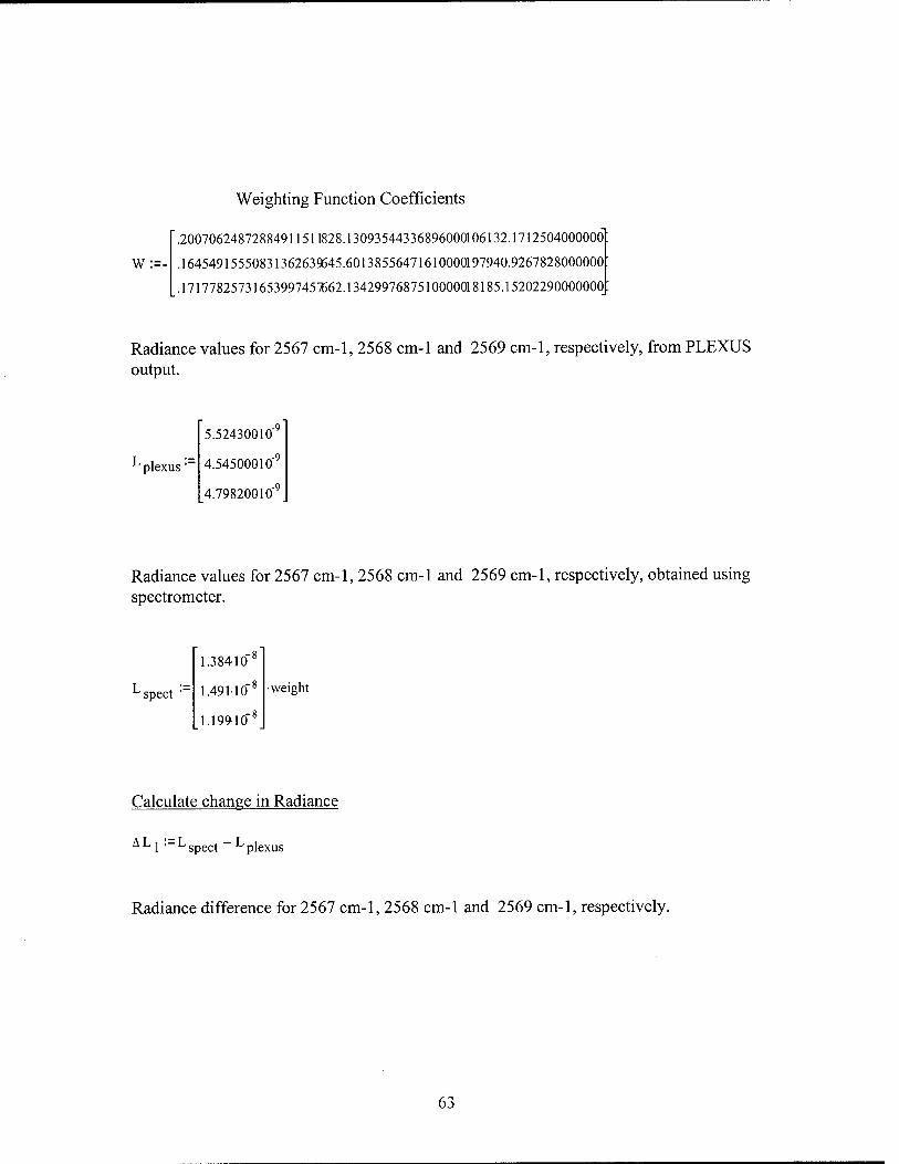
Weighting Function Coefficients

.20070624872884911511828.13093544336896000106132.1712504000000

. 16454915550831362639645.60138556471610000197940.9267828000000

.17177825731653997457562.1342997687510000018185.15202290000000

Radiance values for 2567 cm-1, 2568 cm-1 and 2569 cm-1, respectively, from PLEXUS output.

'plexus'

5.52430010"-

4.54500010"-

4.79820010"'

Radiance values for 2567 cm-1, 2568 cm-1 and 2569 cm-1, respectively, obtained using spectrometer.

' spect

1.38410'

1.49M0":

1.19910"

weight

Calculate change in Radiance

A L1 ' L spect L plexus

Radiance difference for 2567 cm-1, 2568 cm-1 and 2569 cm-1, respectively.

63

AL

i-9 9.3260210

1.14534310"

8.0670710"'

Solving for the change in brightness temperature function, DB(zp, coefficients

coeff j :=W-ALj

coeff 1

■1.896968963650760 rl

3.766163063027040 rll

■2.30036652455620 .-14

a^j :=coeff j

bb] :=coeff j

cbl :-coeff i

lbl 1.896968963650760 r7

bbl = 3.766163063027040

cb] =-2.30036652455620 ,-14

AB1(z):=abl+-bblz+cblz

Brightness temperature function used to calculate initial kernel functions

ab :=3.9076510

64

bb :=-2.00021Ö"4

cb :=- 1.17791Ö"10

db:= 5.9585210

eb:=1.58610"14

fb :=-8.325510"12

gb:=-1.139810"18

hb := 7.9982710"16

ib := 4.305961Ö"23

jb:=-2.743710"20

kb :=-6.78210"28

ab + cbz-|-ebz2-|-gbz3 + ibz4+kbz5

Bplexus(z): j 3 4 5 l + bb + bbz+dbz +fbz +hbz +jfe-z

i :=0.. 55

Calculating B(z) + ABfz)

-l watt) Bl.^1

;=(Bplexus(il000) + ABl(il00°))cm" 2 cm ,

Converting new brightness temperatures into a temperature profile

T, spectrometer '" TVB, i+l

65

spectrometer

1

1 274.82

2 274.21

3 271.75

4 268.97

5 267.3

6 267.53

7 269.52

8 272.57

9 276.03

10 279.51-

11 282.8

12 285.86

13 288.68

14 291.26

15 293.65

16 295.87

K

Calculated Temperatures using spectrometer method

T plexus'

290.233 274.8

286.949 266.2

281.901 262.2

275.579 261.0

268.449 257.7

260.924 K radiosonde ' 252.6

253.355 245.9

246.023 240.0

239.15 233.7

232.909 226.3

227.433 218.1

Plexus inputs

K

Actual Temperatures from radiosonde

h:=l.. 10

Calculate difference between calculated temperature profile and radiosonde temperature profile.

h' spectrometer, radiosonde h

AT:

1

1 0.019066430679402

2 8.0123603635991

3 9.55369440331771

4 7.96902201582952

5 9.60055267729683

6 14.9324461347775

7 23.6155693849379

8 32.5668106084541

9 42.3318372053101

10 53.207175648985

K

66

APPENDIX 3: Radiosonde Data

This appendix contains radiosonde data for the two test cases. Radiosonde data is from

the Wilmington OH radiosonde site, which is, located approximately 30 miles southeast

from were the radiometric data was collected.

1 December 1999 0Q00Z RAOB

TTAA 51001 72426 99998 00058 01007 00309 ////////// 92926 05956 35513 85581 12110 34513 70080 10965 35537 50561 24759 35059 40719 37563 35570 30910 54357 01086 25024 62556 36079 20163 57961 34076 15345 55173 34047 10604 57175 33029 88239 63156 35067 77307 01087 40805 51515 10164 00021 10194 ///// 35529=

UJXX 00KW 010000 72426 TTBB 51000 72426 00998 00058 11987 00960 22850 12110 33830 13510 44822 08564 55820 08375 66748 07988 77678 11362 88612 14563 99581 17964 11565 19960 22517 22962 33462 29756 44400 37563 55279 58556 66239 63156 77198 57162 88173 58967 99159 54972 11134 54176 22100 57175 31313 45202 82307 41414 856//=

8 December 1999 0000Z RAOB

USXX 00KW 080000 72426 TTAA 58001 72426 99986 02247 17005 00209 ///// ///// 92838 02668 ///// 85527 07493 23023 70107 00689 23539 50571 18179 25038 40734 30723 25562 30932 45750 25583 25051 52562 26087 20193 57369 26575 15375 58373 26551 88189 58368 26077 77290 25093 42509 51515 10158 10164 00014 10194 ///// 24029=

UJXX 00KW 080000 72426 TTBB 58000 72426 00986 02247 11975 03458 22935 00656 33925 02668 44917 04674 55860 07296 66850 07493 77837 06873 88739 04286 99478 20977 11460 22966 22442 24736 33422 27316 44389 32321 55383 32157 66376 33160 77353 37156 88323 42358 99285 48737 11276 50547 22250 52562 33189 58368 44155 56775 55133 58974 66/// ///// 77123 61374 88120 61774 31313 45202 82302 41414 00900 51515 10150 10158=

67

Bibliography

BOMEM Inc.The MR Series Documantation Set (1997).

Goody R. M., and Y. L. Yung. Atmospheric Radiation: Theoretical Basis (Second Edition). New York: Oxford University Press, 1989.

Hauser, R.G. Survey of Military Applications for Fourier Transform

Infrared (FTIR) Spectroscopy. MS Thesis, AFIT/GM/ENP/99M-07. School of Engineering Physics, Air Force Institute of Technology (AU), Wright-Patterson AFB OH,AFIT, Febuary 1999:

"PLEXUS." Release 3.0 Version 1.0. CD-ROM. Mission Research Corporation, May 1999

Schanda, E. Physical Fundamentals of Remote Sensing. Heidelberg : Springer-Verlag

Berlin, 1986:

Smith, William L., H. E. Rvercomb, H. B Howell, H. M Woolf, R. 0. Knuteson, R. G. Decker, M. J. Lynch, E. R. Westwater, R.G. Staunch, K. P. Moran, B. Stankov, M. J. Falls, J. Jordan, M. Jacobsen, W. F. Dabberdt, R. McBeth, G. Albright, C. Paneitz, G. Wright, P. T. May, and M. T.Decker. "GAPEX: A Groundbased Atmospheric ProfilingExperiment," Bulletin of the American Meteorological Society, 71:310-318 (March 1990).

Theriault, J. M., "Retrieval of Tropospheric Profiles from IR Emission Spectra: Preliminary Results with the DBIS," SPIE. 2049: 119-128 (1993)

Theriault, J. M., C. Bradatte, and J. Gilbert, Atmospheric Remote Sensing with a Ground- based Spectrometer system. SPIR 2744: 664-672 (1996)

Wallace, P. V. and Peter V. Hobbs. Atmospheric Science An Introductory Survey. New York: Academic Press, Inc., 1977

68

REPORT DOCUMENTATION PAGE Form Approved OMB No. 0704-0188

Public reporting burden for this collection of information is estimated to average 1 hour per response, including the time for reviewing instructions, searching existing data sources, gathering and maintaining the data needed, and completing and reviewing the collection of information. Send comments regarding this burden estimate or any other aspect of this collection of information, including suggestions for reducing this burden, to Washington Headquarters Services, Directorate for Information Operations and Reports, 1215 Jefferson Davis Highway, Suite 1204, Arlington, VA 22202-4302, and to the Office of Management and Budget, Paperwork Reduction Project (0704-0188), Washington, DC 20503.

1. AGENCY USE ONLY (Leave blank) 2. REPORT DATE

March 2000

3. REPORT TYPE AND DATES COVERED

Master's Thesis 4. TITLE AND SUBTITLE

Atmospheric Temperature Profiles By Ground-based Infrared Spectrometer Measurements

6. AUTHOR(S)

Jon M. Saul, First Lieutenant, USAF

5. FUNDING NUMBERS

7. PERFORMING ORGANIZATION NAME(S) AND ADDRESS(ES)

Air Force Institute of Technology Graduate School of Engineering and Management (AFIT/EN) 2950 P Street, Building 640 WPAFB OH 45433-7765

8. PERFORMING ORGANIZATION REPORT NUMBER

AFIT/GM/ENP/00M-11

9. SPONSORING/MONITORING AGENCY NAME(S) AND ADDRESS(ES)

AFRL/VSBM ATTN: Capt Roy Calfas Hanscom AFB, MA 01731 DSN 487-3645

10. SPONSORING/MONITORING AGENCY REPORT NUMBER

11. SUPPLEMENTARY NOTES

Chairman: Lt Col Glenn P. Perram, ENP, DSN: 785-3636, ext. 4511 Member: Dr Mark E. Oxley ENP, DSN: 785-3636, ext. 4645 Member: Major Devin J. Delia-Rose, ENP, DSN: 785-3636, ext. 12a. DISTRIBUTION AVAILABILITY STATEMENT

APPROVED FOR PUBLIC RELEASE; DISTRIBUTION UNLIMITED. 12b. DISTRIBUTION CODE

13. ABSTRACT (Maximum 200 words) A method to recover atmospheric temperature profiles using a ground-based Fourier Transform Infrared spectrometer was investigated. The method used a difference form of the radiative transfer equation, a Bomem MR series Fourier Transform Infrared Spectrometer to collect atmospheric radiance values, and the Phillips Laboratory Expert-assisted User Software (PLEXUS) atmospheric radiance model, to recover an atmospheric temperature profile. The method researched uses radiance values from both the spectrometer measurements and the atmospheric model, along with kernel functions calculated by the atmospheric model as input to a difference form of the radiation transfer equation. From this the change in brightness temperatures was determined. The method assumes that the actual brightness temperature profile is a summation of a standard or reference brightness temperature profile plus some change in the brightness temperature. The brightness temperature profile used by the atmospheric model is the reference brightness temperature profile. Planck's Law was employed to transform the calculated brightness temperature function into a temperature function. A temperature profile was retrieved, although significant differences existed between the recovered temperature profile and a radiosonde recovered temperature profile.

14. SUBJECT TERMS Ground-based Remote Sensing, Spectrometer, Temerature Profiling, Infrared

15. NUMBER OF PAGES

69 16. PRICE CODE

17. SECURITY CLASSIFICATION OF REPORT

UNCLASSIFIED

18. SECURITY CLASSIFICATION OF THIS PAGE

UNCLASSIFIED

19. SECURITY CLASSIFICATION OF ABSTRACT

UNCLASSIFIED

20. LIMITATION OF ABSTRACT

UL Standard Form 298 (Rev. 2-89) (EG) Prescribed by ANSI Std. 239.18 Designed using Perform Pro, WHS/DIOR, Oct 94

Atmospheric Temperature Profiles by Ground-based Infrared ...

Documents

Transcript of Atmospheric Temperature Profiles by Ground-based Infrared ...