Earth Syst. Dynam., 8, 1019–1030, 2017https://doi.org/10.5194/esd-8-1019-2017© Author(s) 2017. This work is distributed underthe Creative Commons Attribution 3.0 License.

Atmospheric teleconnections between the Arctic andthe eastern Baltic Sea regions

Liisi Jakobson1,2, Erko Jakobson2, Piia Post1, and Jaak Jaagus1

1University of Tartu, Tartu, Estonia2Tartu Observatory, Tõravere, Estonia

Correspondence to: Liisi Jakobson (liisi.jakobson@ut.ee)

Received: 31 March 2017 – Discussion started: 6 April 2017Revised: 30 September 2017 – Accepted: 9 October 2017 – Published: 14 November 2017

Abstract. The teleconnections between meteorological parameters of the Arctic and the eastern Baltic Sea re-gions were analysed based on the NCEP-CFSR and ERA-Interim reanalysis data for 1979–2015. The easternBaltic Sea region was characterised by meteorological values at a testing point (TP) in southern Estonia (58◦ N,26◦ E). Temperature at the 1000 hPa level at the TP have a strong negative correlation with the Greenland sec-tor (the region between 55–80◦ N and 20–80◦W) during all seasons except summer. Significant teleconnectionsare present in temperature profiles from 1000 to 500 hPa. The strongest teleconnections between the same pa-rameter at the eastern Baltic Sea region and the Arctic are found in winter, but they are clearly affected by theArctic Oscillation (AO) index. After removal of the AO index variability, correlations in winter were below±0.5,while in other seasons there remained regions with strong (|R|> 0.5, p < 0.002) correlations. Strong correla-tions (|R|> 0.5) are also present between different climate variables (sea-level pressure, specific humidity, windspeed) at the TP and different regions of the Arctic. These teleconnections cannot be explained solely with thevariability of circulation indices. The positive temperature anomaly of mild winter at the Greenland sector shiftstowards east during the next seasons, reaching the Baltic Sea region in summer. This evolution is present at 60and 65◦ N but is missing at higher latitudes. The most permanent lagged correlations in 1000 hPa temperaturereveal that the temperature in summer at the TP is strongly predestined by temperature in the Greenland sectorin the previous spring and winter.

1 Introduction

Over the past half a century, the Arctic has warmed at abouttwice the global rate (IPCC, 2013), a phenomenon called theArctic amplification (AA). At the same time, a significant de-crease in sea ice extent has occurred in all calendar monthssince 1979 (Simmonds, 2015), which has been declared tohave a leading role in recent AA by some scientists (e.g.Screen and Simmonds, 2010; Francis and Vavrus, 2012). Onthe other hand, Perlwitz et al. (2015) disagree with the com-mon assumption that sea ice decline is primarily responsiblefor the amplified Arctic tropospheric warming. They foundthat from October to December, the main factors responsiblefor the Arctic deep tropospheric warming are (1) the recentdecadal fluctuations and (2) long-term changes in sea sur-face temperatures. These two factors are located outside the

Arctic. According to Sato et al. (2014) warm southerly ad-vection is favourable for retreating sea ice over the BarentsSea and warming of air aloft, whereas sea ice decline wouldresult in warming over the Barents Sea because of anoma-lous turbulent heat fluxes. Screen et al. (2012) found thatsea ice concentration and sea surface temperature explain alarge portion of the observed Arctic near-surface warming,whereas remote sea surface temperature changes explain themajority of observed warming aloft. As the energy budgetof the Arctic is highly dependent on energy exchange withlower latitudes, the changes in atmospheric and oceanic cir-culation play an important role in a variety of heat conser-vation changes in the Arctic, most prominently expressed insea ice volume variations. The observed enhanced warmingof the Arctic, referred to as the AA, is expected to be related

Published by Copernicus Publications on behalf of the European Geosciences Union.

1020 L. Jakobson et al.: Atmospheric teleconnections between the Arctic and the eastern Baltic Sea regions

to further changes that impact mid-latitudes and the rest ofthe world (Jung et al., 2015; Walsh, 2014). These Arctic in-fluences could be direct, as the advection of cold and dryair from over the ice-covered areas to the neighbouring ter-ritories, but it could also be through teleconnections – thelarge-scale patterns of high- and low-pressure systems andcirculation anomalies that cover vast geographical areas andreflect the non-periodic oscillations of the climate system.

Teleconnection as a term was first used byÅngström (1935). Wallace and Gutzler (1981) definedteleconnections as significant simultaneous correlationsbetween the time series of meteorological parameters atwidely separated points on the Earth; the essence of ateleconnection is that a climatic process may influence theEarth’s system elsewhere (Liu and Alexander, 2007).

Teleconnections between the Arctic and mid-latitude re-gions have been the focus of research for many years andseveral reviews about the Arctic sea ice impact on the globalclimate (Budikova, 2009; Vihma, 2014) or Eurasian climate(Gao et al., 2015) have been published. Budikova (2009)stated that the size of the response of the climate of re-mote regions to changes in the Arctic has been found to belinked linearly, but the forcing direction non-linearly. Lessice in the Arctic results in a significant decrease in the speedof the westerlies and the intensities of storms poleward of45◦ N (Budikova, 2009). Many studies suggest that the Arc-tic sea ice decline increases the probability for circulationpatterns resembling the negative phase of the Arctic Oscil-lation (AO) and North Atlantic Oscillation (NAO) indices inwinter (Vihma, 2014). However, there is debate as to whetherthe reduction in the autumn Arctic sea-ice-induced negativeAO/NAO index can persist into winter, and it has been sug-gested that winter atmospheric circulation is more closelyassociated with changes in the winter Arctic sea ice (Gaoet al., 2015). Several studies have demonstrated relation-ships between warming and/or ice decline, and mid-latitudeweather and climate extremes (Handorf et al., 2015; Coumouet al., 2014; Tang et al., 2013; Petoukhov et al., 2013; Fran-cis and Vavrus, 2012; Petoukhov and Semenov, 2010). Oth-ers have analysed whether these associations are statisticallyand/or physically robust (Hassanzadeh et al., 2014; Screen etal., 2014; Barnes et al., 2014; Screen and Simmonds, 2013,2014; Barnes, 2013), while some investigations suggest thatthe apparent associations may have their origin, in part, in re-mote influences (Perlwitz et al., 2015; Sato et al., 2014; Pe-ings and Magnusdottir, 2014; Screen et al., 2012; Petoukhovand Semenov, 2010).

The linkages between the Arctic and mid-latitudes dependon geographical region, season, and other impacts. There arecertain geographical regions in the Arctic that have greateramount of warming and the influence of these is more inves-tigated. Arctic warming over the Barents and Kara seas andits impacts on the mid-latitude circulations have been widelydiscussed (Dobricic et al., 2016; Semenov and Latif, 2015;Kug et al., 2015; Sato et al., 2014). Another particular re-

gional warm core (Screen and Simmonds, 2010) is the EastSiberian and Chukchi seas, which is related to severe win-ters over North America (Kug et al., 2015; Lee et al., 2015).Screen and Simmonds (2010) also described the third partic-ular regional warm core – northeast Canada and Greenland –which has been less investigated. Wu et al. (2013) focused onwinter sea ice concentration west of Greenland, including theLabrador Sea, Davis Strait, Baffin Bay, and Hudson Bay, andfound that winter sea ice concentration west of Greenlandis a possible precursor for summer atmospheric circulationand rainfall anomalies over northern Eurasia. If we look atthe regions in the mid-latitudes then potential Arctic telecon-nections with Europe are less clear than with North Amer-ica and Asia (Overland et al., 2015). The linkages betweenthe Arctic and mid-latitudes depend also on season. Summeris exceptional season when the weather conditions are lessaffected by large-scale atmospheric circulation both in mid-latitudes and in the Arctic. But the influence of the increasein late summer open water area is directly contributing to amodification of large-scale atmospheric circulation patterns(Overland and Wang, 2010).

The eastern Baltic Sea region features very variableweather conditions due to its location in the climatic tran-sition zone between the North Atlantic and the Eurasian con-tinent. The region is also close to the Arctic or even part ofit (depending on defining the borderlines) and certainly hasa direct Arctic influence. The weather in the region dependshighly on the position of the polar front: it can be locatednorthward as well as southward of the area. According tothe Second Assessment of Climate Change for the Baltic SeaBasin (BACC II, 2015), significant changes have occurredin climate parameters, which could be associated with large-scale atmospheric circulation. Intensity of the zonal circu-lation, i.e. the westerlies, has increased during the cold pe-riod (NDJFM), especially in February and March. After the1980s there has been significant temperature increase in theBaltic Sea region (BACC II, 2015), which has not been equalthroughout a year. The highest increase in air temperatureis typical for spring (MAM) season. Although a remarkablewarming has also been present in winter (DJF), it is notsignificant due to a very high temporal variability (Jaagus,2006). A tendency of increasing precipitation in winter andspring was detected in the Baltic Sea region during the lat-ter half of the 20th century, possibly increasing the risk ofextreme precipitation events. There is some evidence thatthe intensity of storm surges may have increased in someparts of the Baltic Sea in recent decades, and this has beenattributed to long-term shifts in the tracks of some cyclonetypes rather than to a long-term change in the intensity ofstorminess (BACC II, 2015).

It is known that fluctuations of the climatological param-eters in the Baltic Sea region are strongly affected by theatmospheric circulation variability described by the telecon-nection indices of NAO and AO (BACC II, 2015). There is noclear understanding of the reasons for the changes in these in-

Earth Syst. Dynam., 8, 1019–1030, 2017 www.earth-syst-dynam.net/8/1019/2017/

L. Jakobson et al.: Atmospheric teleconnections between the Arctic and the eastern Baltic Sea regions 1021

dices or climatic parameters in the Baltic Sea region in mostrecent time. One of the reasons for incomplete understandingis the non-stationarity of the NAO spatial pattern and the tem-poral correlations (Lehmann et al., 2011, 2017). It is naturalto assume that changes in the Arctic climate system have aneffect on the eastern Baltic Sea region and vice versa due totheir close proximity. Our aim is to clarify how the climaticparameters in the eastern Baltic Sea and Arctic regions areassociated. Knowledge of such connections helps to defineregions in the Arctic that could be with higher extent associ-ated with the eastern Baltic region climate change.

Our analysis is designed as follows. We selected one gridpoint (the testing point, TP) to represent the eastern BalticSea region and to find correlations between climate param-eters at this point and in the Arctic cap to find the regionsof mutual connections. Next, we calculate the partial corre-lations with various teleconnection indices as control factorsto get rid of the known atmospheric circulation variability. Tocompare broad atmospheric circulation patterns, we calculategeopotential heights differences between cold and mild win-ters. Due to longer memory of non-atmospheric componentsof climate system we compute by season-lagged correlationsbetween climate parameters.

The objective of this paper is to indicate the relationshipsbetween meteorological parameters of the Arctic region andthe TP. By tracking down the teleconnections between therapidly changing Arctic region and the TP we can get valu-able information about possible future trends in the easternBaltic Sea region even if the changes in both regions werecaused by a third factor.

2 Data and methodology

We used monthly mean reanalysis data from the ClimateForecast System Reanalysis (CFSR) on a 0.5◦× 0.5◦ hori-zontal grids provided by the National Centers for Environ-mental Prediction (NCEP). For the period 1979–2010, 6-hourly data of CFSR version 1 (Saha et al., 2010) were usedfor calculating monthly means; for 2011–2015, 6-hourly dataof CFSR version 2 were used (Saha et al., 2014). For repro-ducibility, we repeated all calculations using ERA-Interimdata (Dee et al., 2011). Mostly, these two models showedvery similar results. In this paper, only NCEP-CFSR resultsare shown, only disagreements between models are pointedout in the Results section. The following parameters wereanalysed: temperature at 1000, 850, 500, and 250 hPa level;sea-level pressure (SLP); geopotential heights from 1000 to100 hPa; specific humidity and wind speed at 1000 hPa; andsea ice concentration (SIC). Monthly means and seasonalmeans (DJF, MAM, JJA, SON) were calculated from the 6-hourly data. Monthly mean wind speed was calculated as ascalar average.

The teleconnection indices we applied in our analyseswere chosen according to the possible influence due to thegeographical position of the centres of action of the tele-connection patterns over the North Atlantic–Eurasian region.The following indices were chosen: (1) the North AtlanticOscillation (NAO), which is the dominant mode of atmo-spheric variability in the North Atlantic sector throughout theyear (Barnston and Livezey, 1987); (2) the Arctic Oscillation(AO), which is usually defined as the first EOF (empirical or-thogonal function) of the mean sea-level pressure field in theNorthern Hemisphere (Ambaum et al., 2001); (3) the Scan-dinavian pattern (SCA), which consists of a primary circu-lation centre over Scandinavia, with two other weaker cen-tres of action with the opposite sign, one over the north east-ern Atlantic and the other over central Siberia to the south-west of Lake Baikal (Bueh and Nakamura, 2007); (4) theEast Atlantic pattern (EA), which consists of a north–southdipole of anomaly centres spanning the North Atlantic fromeast to west (Barnston and Livezey, 1987); (5) the East At-lantic/West Russia pattern (EA/WR), which consists of fourmain anomaly centres: Europe, northern China, central NorthAtlantic, and north of the Caspian Sea; (6) the Polar/Eurasiapattern (PEU) consists of height anomalies over the polar re-gion, and opposite anomalies over northern China and Mon-golia. (7) Additionally, Pacific Decadal Oscillation (PDO),which is the dominant year-round pattern of monthly NorthPacific sea surface temperature (SST) variability, was in-cluded. Although its geographical centres are far from theBaltic Sea region, Uotila et al. (2015) found that PDO corre-lated significantly with the ice concentration and temperatureof Baltic Sea. All indices were downloaded from the NOAA-CPC database (http://www.cpc.noaa.gov).

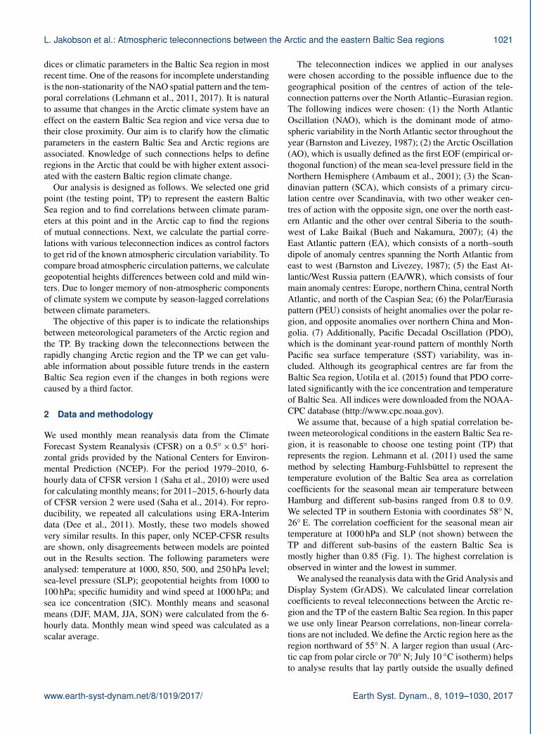
We assume that, because of a high spatial correlation be-tween meteorological conditions in the eastern Baltic Sea re-gion, it is reasonable to choose one testing point (TP) thatrepresents the region. Lehmann et al. (2011) used the samemethod by selecting Hamburg-Fuhlsbüttel to represent thetemperature evolution of the Baltic Sea area as correlationcoefficients for the seasonal mean air temperature betweenHamburg and different sub-basins ranged from 0.8 to 0.9.We selected TP in southern Estonia with coordinates 58◦ N,26◦ E. The correlation coefficient for the seasonal mean airtemperature at 1000 hPa and SLP (not shown) between theTP and different sub-basins of the eastern Baltic Sea ismostly higher than 0.85 (Fig. 1). The highest correlation isobserved in winter and the lowest in summer.

We analysed the reanalysis data with the Grid Analysis andDisplay System (GrADS). We calculated linear correlationcoefficients to reveal teleconnections between the Arctic re-gion and the TP of the eastern Baltic Sea region. In this paperwe use only linear Pearson correlations, non-linear correla-tions are not included. We define the Arctic region here as theregion northward of 55◦ N. A larger region than usual (Arc-tic cap from polar circle or 70◦ N; July 10 ◦C isotherm) helpsto analyse results that lay partly outside the usually defined

www.earth-syst-dynam.net/8/1019/2017/ Earth Syst. Dynam., 8, 1019–1030, 2017

1022 L. Jakobson et al.: Atmospheric teleconnections between the Arctic and the eastern Baltic Sea regions

Figure 1. Correlation maps of air temperature at the 1000 hPa levelfor the testing point in the Baltic Sea region.

Arctic region. For correlations with the TP, the first correla-tion input was taken at the TP and the second in the Arcticregion.

All presented correlations are significant at the confidencelevel 95 %; only strong correlations |R|> 0.5 are discussedin this paper. We used F tests to assess the significance ofcorrelations. Autocorrelation in the time series is taken intoaccount by using effective number of degrees of freedom forcorrelation, calculated using lag-one autocorrelation of resid-uals. For comparison of averages, we used t tests assumingequal variances.

Detrending of seasonal time series was done to ascertainthat the correlations are not caused by mutual trends in inputvariables using the following formula:

Yi =Xi − (k · year+ b−Xaverage).

Therefore, linear trends for each parameter at each grid pointwere calculated for each season and all correlations werecalculated twice – first using the regular and second the de-trended data. Detrending did not change general patterns ofcorrelations with TP – only negative correlation in the Green-land region intensified slightly. All discussed correlations ofthe regular data were also significant in analysis of detrendeddata. As we are exploring the connections that include long-term climatic trends such as global warming, we present inthis paper only correlations of the regular, non-detrendeddata.

The next step in the analysis was to remove from the corre-lations the effect of atmospheric teleconnections which couldbe described by known teleconnection indices. For that pur-pose, partial correlations between selected atmospheric vari-ables with the controlling effect of the teleconnection indiceswere calculated as follows:

RAB|C =RAB −RAC ·RBC√

(1−R2AC) · (1−R2

BC).

Cold and mild winters were defined as years when the winteraverage temperature differed the whole period average morethan one standard deviation at a geographical point in theGreenland sector (70◦ N, 60◦W). Accordingly, cold winterswere 1983, 1984, 1989, 1990, 1992, and 1993; mild winterswere 1980, 1985, 1986, 2003, 2007, 2009, 2010, and 2011.

The last phase of the analysis was to calculate the laggedcorrelation coefficients with the purpose of revealing the pos-sible delayed dependences between the atmospheric vari-ables of the Arctic region and the TP. For the lagged corre-lation, the second parameter was taken by lag months earlierthan the first parameter.

3 Results

3.1 Spatial correlations of climatic variables

Climatic variables at separate grid points are usually not in-dependent, but correlations in space depend highly on thedistance and climatic variables. For example, for tempera-ture, the dependence in space stays significant for longer dis-tances than for precipitation as the processes of their forma-tion are different. But besides the short distance correlationof climatic parameters between the TP and the surroundinggrid points, there are also vast areas far from the TP, still hav-ing significant correlations (Fig. 2). The strongest correla-tions are detected in winter when temperature at the 1000 hPalevel at the TP has a positive correlation over a large area,covering nearly the whole northern Eurasia, with the maxi-mum (R > 0.5) in northern Europe, on the eastern EuropeanPlain and in central Siberia. At the same time, an area of astrong negative correlation (R <−0.5) is found in the Green-land sector. Hereinafter, we define the Greenland sector asregion between 55–80◦ N and 20–80◦W. A similar correla-tion pattern, but of lower magnitude, is also present in springand autumn. The pattern of spatial correlation for tempera-ture at the 1000 hPa level in summer is different. The areaof positive correlation is much smaller than in winter, mostlycovering only Europe, but a negative correlation is detectedin the central Arctic and western Siberia.

Specific humidity at the 1000 hPa level has a similar pat-tern of correlations to temperature in the same seasons. Thelargest differences are observed in Siberia in spring withabout 20 % higher correlation in temperature than in specifichumidity. Wind speed at the 1000 hPa level at the TP has thehighest correlation in winter, while the areas of a positivecorrelation in Europe and North Atlantic and of a negativecorrelation in the central Arctic and the Greenland sector arestrictly distinct. During the other seasons the spatial corre-lation is much lower. There is a strong positive correlation

Earth Syst. Dynam., 8, 1019–1030, 2017 www.earth-syst-dynam.net/8/1019/2017/

L. Jakobson et al.: Atmospheric teleconnections between the Arctic and the eastern Baltic Sea regions 1023

Figure 2. Correlation maps between seasonal mean 1000 hPa temperature (t1000), specific humidity (q1000), wind speed (s1000), and SLPmeasured at the TP (the yellow circle) and in the whole Arctic region. Columns represent seasons; all presented correlations are significantat the confidence level 95 %. The Greenland sector (20–80◦W, 55–80◦ N) borders are marked with two yellow lines.

Table 1. Areal average and minimum and maximum of seasonal correlations between VAR1 at TP and VAR2 at the Greenland sector(20–80◦W, 55–80◦ N).

Average Minimum Maximum

VAR1 VAR2 DJF MAM JJA SON DJF MAM JJA SON DJF MAM JJA SON

t1000 t1000 −0.41 −0.23 0.15 −0.02 −0.63 −0.51 −0.22 −0.49 0.03 0.21 0.44 0.49t850 t850 −0.41 −0.26 0.09 −0.02 −0.63 −0.46 −0.19 −0.34 0.08 0.06 0.34 0.48t500 t500 −0.32 −0.19 0.24 0.00 −0.52 −0.51 0.02 −0.20 0.09 0.15 0.49 0.40t250 t250 0.31 0.20 −0.02 0.00 0.08 0.02 −0.36 −0.29 0.55 0.39 0.41 0.28q1000 q1000 −0.44 −0.20 0.28 −0.04 −0.65 −0.50 −0.19 −0.53 0.11 0.09 0.62 0.45s1000 s1000 −0.11 0.02 0.05 0.01 −0.72 −0.58 −0.47 −0.36 0.77 0.67 0.75 0.42SLP SLP 0.15 −0.12 −0.25 −0.36 −0.25 −0.30 −0.43 −0.54 0.51 0.33 0.16 −0.13t1000 SLP −0.39 −0.27 −0.23 0.03 −0.73 −0.50 −0.42 −0.45 0.35 0.11 −0.02 0.51t1000 s1000 −0.15 −0.03 −0.02 −0.03 −0.67 −0.54 −0.42 −0.65 0.65 0.48 0.38 0.43t1000 icec 0.17 0.11 −0.07 0.01 −0.26 −0.34 −0.62 −0.41 0.61 0.64 0.41 0.48s1000 icec 0.19 0.06 0.03 0.16 −0.28 −0.67 −0.36 −0.24 0.63 0.63 0.71 0.59

in wind speed in summer between the TP and the CanadianArctic Archipelago and the Bering Sea region. SLP at the TPhas a significant negative correlation with SLP in the Green-land sector in autumn. Figure 2 using ERA-Interim data (notshown) gave very similar results. Detectable differences werefound in central Arctic in summer and autumn when corre-lations with temperature and specific humidity were slightlyhigher in ERA-Interim than NCEP-CFSR.

The Greenland sector showed most often significant corre-lations with the parameters of the eastern Baltic Sea region.In Table 1 are given spatial average, minimum, and maxi-mum values of seasonal correlations between the TP and theGreenland sector. Strong negative correlation in the Green-

land sector at 1000 hPa temperature in winter and spring de-creases with altitude and turns even positive at 250 hPa (Ta-ble 1). Specific humidity at 1000 hPa shows quite similar val-ues with temperature at the same level (Table 1). The cor-relation between wind speed at 1000 hPa at the TP and theGreenland sector is mostly negative in winter (Fig. 2), reach-ing up to −0.72 (Table 1). The most significant correlationbetween SLP is present in autumn and summer (Fig. 2, Ta-ble 1).

Climatic variables have close relationships between them-selves. If there is a climatic change in one parameter, for ex-ample in temperature, then it also causes changes in otherparameters connected with it, for example in ice concentra-

www.earth-syst-dynam.net/8/1019/2017/ Earth Syst. Dynam., 8, 1019–1030, 2017

1024 L. Jakobson et al.: Atmospheric teleconnections between the Arctic and the eastern Baltic Sea regions

Table 2. Areal average of seasonal (winter and spring) partial cor-relations between 1000 hPa temperature at TP and the Greenlandsector (20–80◦W, 55–80◦ N) using different teleconnection indicesas controlling factors.

Index DJF MAM

reg. correl. −0.41 −0.23AO −0.07 −0.10NAO −0.10 −0.11PDO −0.45 −0.26CAI −0.41 −0.21PEU −0.42 −0.18EA −0.43 −0.27EA/WR −0.41 −0.22SCA −0.25 −0.23

tion. Similarly to correlations of the same climate variableat the TP and the Arctic (Fig. 2), there are strong correla-tions (|R|> 0.5) between different climate variables at theTP and the Greenland sector (Table 1). Correlation betweenthe 1000 hPa temperature at the TP and SLP shows expectedresults with a positive correlation in summer and negative inwinter around the TP (not shown). Largest correlations withthe Greenland sector are in winter, when the correlation ison average −0.39 and extremal values reach even to −0.73.Correlations with ice concentration have quite large extremalvalues, reaching up to 0.71 in summer for wind speed and0.64 in spring for temperature, but these correlations are sig-nificant only at narrow coastal areas around Greenland (notshown).

3.2 Impact of the teleconnection indices

To analyse the impact of the seven teleconnection indicesgiven in Sect. 2, the average of partial correlations between1000 hPa temperature at TP and the Greenland sector (55–80◦ N, 20–80◦W) are shown for winter and spring in Table 2.The influence of teleconnection indices depends strongly ona season and a parameter. Larger difference from regular cor-relation values means higher impact of the index. Accordingto the definition, removing the impact may decrease, but mayalso increase, the correlation.

The first row of Table 2 shows the average of the regularPearson correlation of temperature at 1000 hPa in the region.It has the most significant values during winter and spring.Also, the impact of AO and NAO is most considerable duringthese seasons. Considering the correlation coefficients be-tween seasonal mean temperatures, specific humidity, windspeed at the 1000 hPa level and SLP at the TP, the AO in-dices have mostly higher correlations than the NAO indices;only in summer and autumn does SLP have a significantlyhigher correlation with the NAO index (not shown). Here-after mostly only the AO index is analysed (and not the NAOindex).

Figure 3. Seasonal difference maps (years with mild winters mi-nus years with cold winters) in air temperature at 1000 hPa level(shading with confidence level of 95 %), and geopotential height at500 hPa level (contours).

Partial correlations with the controlling factor AO indexreduce the area with a statistically significant correlationaround the TP in all parameters and in all seasons. This ef-fect on the remote areas depends on the season. In winterthe effects of the AO indices on spatial correlations are thestrongest, up to 0.5. In spring, the differences between partialcorrelations with the AO indices are below 0.2 in the wholeregion compared to the regular correlations between the TPand the Arctic. In summer and autumn, the differences areeven smaller than in spring.

Partial correlation in temperature, removing the influenceof the AO index, is below ±0.5 at all levels (1000, 850, 500,and 250 hPa) in winter, though the regular correlations are thestrongest (not shown). In other seasons, regions with strongerpartial correlations than ±0.5 remain. In summer and au-tumn, the AO indices have no significant influence on cor-relations on higher altitudes, similarly to the 1000 hPa level.

The impact of other teleconnection indices than AO andNAO is much smaller. Among other indices the SCA indexhas the strongest impact in winter but very small impact dur-ing other seasons, while in spring the partial correlation withthe PEU index decreases the value of correlation coefficientthe most (except AO and NAO). The average (regular) corre-lation coefficients between 1000 hPa temperature at TP andthe Greenland sector during summer and autumn were only0.15 and −0.02, respectively, and are not discussed here.

3.3 Comparison of winters with low and hightemperature

To compare broad atmospheric circulation patterns, we turnto the difference map of the geopotential heights of 500 hPa

Earth Syst. Dynam., 8, 1019–1030, 2017 www.earth-syst-dynam.net/8/1019/2017/

L. Jakobson et al.: Atmospheric teleconnections between the Arctic and the eastern Baltic Sea regions 1025

Figure 4. Differences in the mean geopotential heights between mild and cold winters along the 60◦W vertical slice. Contour intervals are10 gpm; blue represents negative height differences and red positive height differences.

and temperature at 1000 hPa by subtracting the compositesof cold winters (DJF) from those of mild winters (Fig. 3).The large-scale atmospheric circulation pattern in Fig. 3shows that the geopotential heights of 500 hPa are more than100 gpm higher in mild winters than in cold ones. The maxi-mum of this height anomaly is centred over the maximum ofthe 1000 hPa temperature difference. The whole column (upto 500 hPa) of the air in the Greenland sector is warmer thanat cold years. Coming down to the lower surfaces (700 hPa,SLP, not shown), the maximum height anomaly is shifted tothe east. Ensuing spring and summer also show positive val-ues of the 1000 hPa temperature and the geopotential heightsof 500 hPa in the Greenland sector (spring and summer inFig. 3). In autumn the positive anomaly of 1000 hPa tem-perature and geopotential heights of 500 hPa are present inSiberia.

Along the 60◦W vertical slice the spring atmosphere ex-hibits a baroclinic structure between about 60 and 82◦ N dueto negative height anomalies in the lower troposphere belowthe 850 hPa and with further higher the positive ones (springin Fig. 4). Similarly to Wu et al. (2013) the vertical distribu-tion of spring height anomalies differs from that of the pre-vious winter when height anomalies show dominantly quasi-barotropic structure. The annual evolution of 500 hPa heightdifferences at 60◦ N shows that the positive height anomalyat the Greenland sector shifts towards east during the nextseasons, reaching Scandinavia–Baltic Sea region in summer(Fig. 5). The propagation of the mid-tropospheric anomaliesin this region is non-linear: these height anomalies are signif-

Figure 5. Evolution of 500 hPa height differences between mild andcold winters at 60◦ N; red and blue shading indicates differences atthe 95 % significance levels for positive and negative height, respec-tively.

icant only over some areas and months, and in May they areslightly negative. Also, at 65◦ N the similar pattern is present(not shown), but at 70 and 75◦ N this kind of signal propa-gation is missing. ERA-Interim has similar patterns at 60◦ N,but without considerable positive difference at the Greenlandsector in winter (not shown).

www.earth-syst-dynam.net/8/1019/2017/ Earth Syst. Dynam., 8, 1019–1030, 2017

1026 L. Jakobson et al.: Atmospheric teleconnections between the Arctic and the eastern Baltic Sea regions

Figure 6. Lagged correlation maps between the TP (the yellow circle) and Arctic 1000 hPa temperature: first row, lag is 0 months (no lag);second row, lag is 3 months; third row, lag is 6 months; fourth row, lag is 9 months. Columns represent seasons; all presented correlationsare significant at the confidence level 95 %.

3.4 Teleconnection using lagged data

The climate system consists of various interactive compo-nents that have highly various response times. The estimatedtimescales in the atmosphere grow with height and reachup to months, but due to atmospheric interactions with theoceans and cryosphere, the conditions in the atmosphere mayhave even longer response times. For finding the effect ofthe previous seasons on atmospheric conditions at the TP,lagged correlations were calculated for the 1000 hPa tem-perature (Fig. 6). The results show that the previous winterseason has a strong effect on temperature during the follow-ing spring (lag= 3) and summer (lag= 6). At the same time,the winter mean temperature has almost no dependence onweather conditions during the previous seasons; there is onlya small region with strong negative correlation in the Taimyrregion in the previous summer (lag= 6). There is a strong(R > 0.5) positive correlation between the 1000 hPa temper-atures at the TP in spring and in Eurasia during the previouswinter (lag= 3). The spring temperature is determined by thetemperature of neither the previous autumn (lag= 6) nor theprevious summer (lag= 9). Summer temperature at the TPhas a strong positive correlation in the Greenland sector withthe previous spring (lag= 3), winter (lag= 6), and autumn(lag= 9). Autumn temperature at the TP has a strong neg-ative correlation with the Fram Strait in the previous sum-mer (lag= 3) and the Taimyr region in the previous winter(lag= 9).

4 Discussion

There are vast areas in the Arctic far from the eastern BalticSea region that show significant correlations with meteoro-logical parameters at the TP. Temperature at the 1000 hPalevel at the TP has a strong positive correlation (R > 0.5)with the eastern European Plain up to central Siberia and astrong negative correlation with the Greenland sector duringall seasons except summer (Fig. 2). These patterns are simi-lar to the correlations with the AO index (not shown) and areprobably partly induced by the general circulation of the at-mosphere. These correlations can be considered as an effectof stronger westerlies that carry relatively warm and moist airfrom the North Atlantic into Eurasia and, at the same time,cold and dry air from the central Arctic to Greenland and theCanadian Arctic Archipelago. As specific humidity and tem-perature are strongly coupled, specific humidity has a similarpattern of correlations as temperature. Warmer air can holdmuch more water vapour. The reason why summer seasondiffers from other seasons maybe caused by a less effectivelarge-scale circulation. Also, the circumstances are differentin summertime. In summer the atmospheric energy budget ispositive, there are more specific humidity and clouds, and themelting ice temperature is conserved by the melting energyof ice. Consequently, we assume that weather conditions insummer are more influenced by local factors, such as dif-ferences in local radiation and heat balances determined bylocal geographical peculiarities, and less affected by large-scale atmospheric circulation.

Earth Syst. Dynam., 8, 1019–1030, 2017 www.earth-syst-dynam.net/8/1019/2017/

L. Jakobson et al.: Atmospheric teleconnections between the Arctic and the eastern Baltic Sea regions 1027

Partial correlation analyses were used as the control for thepotential effects of different teleconnection indices on corre-lations between meteorological parameters at the TP and theArctic. Partial correlations with the controlling factors of theAO and NAO indices had the strongest influence on the cor-relations between meteorological parameters between the TPand the Arctic region; other teleconnection indices had muchsmaller influence (Table 2). Budikova (2012) suggests thatthe AO and NAO are very closely related and the NAO isfrequently referred to as a “local expression” of the AO as itdominates its structure in the Atlantic sector. Still, some sci-entists show different impact of NAO and AO to meteorolog-ical parameters and phenomenon. According to the reviewarticle by Bader et al. (2011), the NAO is the most importantteleconnection index for investigating the impact of the Arc-tic sea ice changes on teleconnection patterns. The study ofAmbaum et al. (2001) suggests also that because of the phys-ical background of the NAO index it may be physically morerelevant and robust for the Northern Hemisphere variabilitythan is the AO index. Uotila et al. (2015) preferred NAO toAO analysing Baltic Sea ice conditions because of the centreof action that has more influence over the Baltic Sea ice con-ditions (Uotila et al., 2015). Thompson and Wallace (1998)claimed that the AO index is actually more strongly cou-pled to the Eurasian winter surface air temperature than theNAO index. Rinke et al. (2013) showed through the coupledregional climate model experiments that atmospheric large-scale circulation in a winter following low September sea iceresemble a negative AO pattern. Our results show that for thecorrelation coefficients between the eastern Baltic Sea regionand the Greenland sector, the AO index had mostly the high-est impact in every season; only in summer and autumn didSLP have a significantly stronger impact with the NAO in-dex. The strongest teleconnections between the same param-eter at the eastern Baltic Sea region and the Arctic region canbe found in winter, but they are clearly affected by the AOindex (Table 2).

Among other teleconnection indices (except AO andNAO) the SCA index showed the largest impact between1000 hPa temperature at TP and the Greenland sector duringwinter (Table 2). The SCA pattern has been shown to influ-ence precipitation, temperatures, and cyclone activity acrossnorthern Europe and Eurasia (Moore et al., 2013; Bueh andNakamura, 2007; Seierstad et al., 2007). Uotila et al. (2015)found that the PDO index has significant impact on the BalticSea ice concentration although physical mechanisms linkingthe Baltic Sea ice with PDO are not well known (Vihma etal., 2014). We investigated the correlation between 1000 hPatemperature at TP and the Greenland sector and removingthe influence of PDO (by partial correlation) did not changethe results much during any season. Removing the EA/WRindex influenced the results even less although regionallythe anomaly centres of the EA/WR pattern include Europeand North Atlantic. Lim (2015) analysed the EA/WR (1979–2012) and found that the positive (negative) EA/WR is asso-

ciated with a strong cooling (warming) over the Ural Moun-tains of northern Russia which is much further to the east ofour TP.

The comparison of 700 and 500 hPa geopotential heightdifferences between mild and cold winters showed that700 hPa geopotential height is shifted to the east. This couldbe due to warmer sea surface of the North Atlantic comparedto the regions that lie to west of it. The positive tempera-ture anomaly at 1000 hPa height shifts from the Greenlandsector in winter towards east reaching to Scandinavia/BalticSea region in summer. This could be also followed by ourlagged analyses which show that the summer temperature atTP has significant correlation with Greenland sector in win-ter (JJA; lag= 6). According to Wu et al. (2013) the summeratmospheric circulation anomalies in the northern Eurasiaare associated with the previous winter SIC west of Green-land. The mechanism is based on a horseshoe-like pattern ofSST anomalies in the North Atlantic that persists in winterand spring. Such an anomaly impacts on ensuing spring at-mosphere over the North Atlantic which links winter–springSIC and SST anomalies and summer atmospheric circulationanomalies over northern Eurasia, including the Baltic Sea re-gion. This proposed mechanism supports our results.

5 Conclusions

Rapid warming and reduction of sea ice is going on in theArctic. In this article, the relations between meteorologicalparameters of the Arctic region and the eastern Baltic Searegion are investigated, using the NCEP-CFSR and ERA-Interim reanalysis data for 1979–2015. The eastern BalticSea region is characterized by meteorological values at thetesting point (TP) in southern Estonia (58◦ N, 26◦ E). Thereare vast areas in the Arctic, far from the eastern Baltic Searegion, that show significant correlations with climatologicalparameters at the TP. The most important findings about theArctic teleconnections with the eastern Baltic Sea region areas follows:

– The strongest teleconnections between the same param-eter in the eastern Baltic Sea region and the Arctic are inwinter, but they are clearly affected by the Arctic Oscil-lation index (AO index). After removal of the AO indexvariability, correlations in winter were below 0.5, whilein other seasons strong (|R|> 0.5) correlations mostlyremain.

– Strong teleconnections are present in temperature pro-files from 1000 to 500 hPa. Similarly to the 1000 hPalevel, teleconnections on higher levels are connectedwith the AO index variability in winter.

– Strong teleconnections are present between differentclimate variables at the TP and the Arctic. Tempera-ture and wind speed at the 1000 hPa level in the eastern

www.earth-syst-dynam.net/8/1019/2017/ Earth Syst. Dynam., 8, 1019–1030, 2017

1028 L. Jakobson et al.: Atmospheric teleconnections between the Arctic and the eastern Baltic Sea regions

Baltic Sea region have, in all seasons, strong telecon-nections with the sea ice concentration in some regionsof the Arctic Ocean. These teleconnections cannot beexplained solely with the climate indices’ variability.

– The annual evolution of 500 hPa height differences (be-tween mild and cold winter in the Greenland sector) at60◦ N shows that the positive temperature anomaly dur-ing winter shifts towards east during the next seasons,reaching to Scandinavia/Baltic Sea region in summer.Also, at 65◦ N the similar pattern is present. At higherlatitudes (70 and 75◦ N) this kind of signal propagationis missing.

– In all seasons there are strong teleconnections in tem-perature at 1000 hPa at the TP with some Arctic regionsfrom the previous seasons. The most permanent laggedcorrelations in 1000 hPa temperature are in summer atthe TP with the Greenland sector in the previous spring,winter, and even autumn.

In conclusion, in every season there are some regions inthe Arctic that have strong teleconnection (|R|> 0.5, p <

0.002) with temperature, SLP, specific humidity, and windspeed in the eastern Baltic Sea region. These relationshipscan be explained by the AO index variability only in winter.In other seasons there must be other influencing factors. Thepositive temperature anomaly evolution of 500 hPa heightdifferences from the Greenland sector in winter to the BalticSea region in summer is present at the 60 and 65◦ N merid-ian and missing at higher latitudes. The lagged correlation in1000 hPa temperature in summer at the TP supports the re-sults of temperature evolution. The results of this study arevaluable for selecting regions in the Arctic that have the sta-tistically largest effect on climate in the eastern Baltic Searegion.

Data availability. The reanalyses data used here are availablefrom the NCAR-UCAR Research Data Archive (https://rda.ucar.edu/) under their data policy rules.

Competing interests. The authors declare that they have no con-flict of interest.

Special issue statement. This article is part of the special issue“Multiple drivers for Earth system changes in the Baltic Sea re-gion”. It is a result of the 1st Baltic Earth Conference, Nida, Lithua-nia, 13–17 June 2016.

Acknowledgements. Comments of four anonymous reviewershave led to a significant improvement of this paper. This study wassupported by the Estonian Research Council grant PUT (645) andinstitutional research funding IUT (2-16) and IUT (20-11) of the

Estonian Ministry of Education and Research. ECMWF, NCAR,and NOAA-CPC are acknowledged for data supply.

Edited by: Marcus ReckermannReviewed by: four anonymous referees

References

Ambaum, M. H. P., Hoskins, B. J., Stephenson, D. B.:Arctic Oscillation or North Atlantic Oscillation?, J.Climate, 14, 3495–3507, https://doi.org/10.1175/1520-0442(2001)014<3495:AOONAO>2.0.CO;2, 2001.

Ångström, A.: Teleconnections of Climatic Changesin Present Time, Geogr. Ann., 17, 242–258,https://doi.org/10.2307/519964, 1935.

BACC II Author Team: Second Assessment of Climate Change forthe Baltic Sea Basin, Springer Open, Berlin, p. 501, 2015.

Bader, J., Mesquita, M. D. S., Hodges, K. I., Keenlyside, N., Øster-hus, S., and Miles, M.: A review on Northern Hemisphere sea-ice, storminess and the North Atlantic Oscillaion: Observationsand projected changes, Atmos. Res., 101, 809–834, 2011.

Barnes, E. A.: Revisiting the evidence linking Arctic Amplifica-tion to extreme weather in midlatitudes, Geophys. Res. Lett., 40,4728–4733, https://doi.org/10.1002/grl.50880, 2013.

Barnes, E. A., Etienne, D. S., Giacomo, M., andWoollings, T.: Exploring recent trends in Northern Hemi-sphere blocking, Geophys. Res. Lett., 41, 638–644,https://doi.org/10.1002/2013GL058745, 2014.

Barnston, A. G. and Livezey, R. E.: Classification, seasonality andpersistence of low-frequency atmospheric circulation patterns,Mon. Weather Rev., 115, 1083–1126, 1987.

Budikova, D.: Role of Arctic Sea Ice in Global AtmosphericCirculation: A review, Global Planet. Change, 68, 149–163,https://doi.org/10.1016/j.gloplacha.2009.04.001, 2009.

Budikova, D.: Northern Hemisphere Climate Variability: Charac-ter, Forcing Mechanisms, and Significance of the North At-lantic/Arctic Oscillation, Geography Compass, 6/7, 401–422,https://doi.org/10.1111/j.1749-8198.2012.00498.x, 2012.

Bueh, C. and Nakamura, H.: Scandinavian pattern and its cli-matic impact, Q. J. Roy. Meteor. Soc., 133, 2117–2131,https://doi.org/10.1002/qj.173, 2007.

Coumou, D., Petoukhov, V., Rahmstorf, S., Petri, S., andSchellnhuber, H. J.: Quasi-resonant circulation regimes andhemispheric synchronization of extreme weather in bo-real summer, P. Natl. Acad. Sci. USA, 111, 12331–12336,https://doi.org/10.1073/pnas.1412797111, 2014.

Dee, D. P., Uppala, S. M., Simmons, A. J., Berrisford, P., Poli,P., Kobayashi, S., Andrae, U., Balmaseda, M. A., Balsamo, G.,Bauer, P., Bechtold, P., Beljaars, A. C. M., van de Berg, L., Bid-lot, J., Bormann, N., Delsol, C., Dragani, R., Fuentes, M., Geer,A. J., Haimberger, L., Healy, S. B., Hersbach, H., Hólm, E. V.,Isaksen, L., Kållberg, P., Köhler, M., Matricardi, M., McNally,A. P., Monge-Sanz, B. M., Morcrette, J.-J., Park, B.-K., Peubey,C., de Rosnay, P., Tavolato, C., Thépaut, J.-N., and Vitart, F.: TheERA-Interim reanalysis: Configuration and performance of thedata assimilation system, Q. J. Roy. Meteor. Soc., 137, 553–597,https://doi.org/10.1002/qj.828, 2011.

Earth Syst. Dynam., 8, 1019–1030, 2017 www.earth-syst-dynam.net/8/1019/2017/

L. Jakobson et al.: Atmospheric teleconnections between the Arctic and the eastern Baltic Sea regions 1029

Dobricic, S., Vignati, E., and Russo, S.: Large-Scale AtmosphericWarming in Winter and the Arctic Sea Ice Retreat, J. Climate, 29,2869–2888, https://doi.org/10.1175/JCLI-D-15-0417.1, 2016.

Francis, J. A. and Vavrus, S. J.: Evidence linking Arctic amplifica-tion to extreme weather in mid-latitudes, Geophys. Res. Lett., 39,L06801, https://doi.org/10.1029/2012GL051000, 2012.

Gao, Y., Sun, J., Li, F., He, S., Sandven, S., Yan, Q., Zhang, Z.,Lohmann, K., Keenlyside, N., Furevik, T., and Suo, L.: Arcticsea ice and Eurasian climate: A review, Adv. Atmos. Sci., 32,92–114, https://doi.org/10.1007/s00376-014-0009-6, 2015.

Handorf, D., Jaiser, R., Dethloff, K., Rinke, A., and Cohen, J.:Impacts of Arctic sea ice and continental snow cover changeson atmospheric winter teleconnections, Geophys. Res. Lett., 42,2367–2377, https://doi.org/10.1002/2015GL063203, 2015.

Hassanzadeh, P., Kuang, Z., and Farrell, B. F.: Responses of mid-latitude blocks and wave amplitude to changes in the meridionaltemperature gradient in an idealized dry GCM, Geophys. Res.Lett., 41, 5223–5232, https://doi.org/10.1002/2014GL060764,2014.

IPCC: Climate Change 2013: The Physical Science Basis. Con-tribution of Working Group I to the Fifth Assessment Re-port of the Intergovernmental Panel on Climate Change,edited by: Stocker, T. F., Qin, D., Plattner, G.-K., Tignor,M., Allen, S. K., Boschung, J., Nauels, A., Xia, Y., Bex,V., and Midgley, P. M., Cambridge University Press, Cam-bridge, United Kingdom and New York, NY, USA, 1535 pp.,https://doi.org/10.1017/CBO9781107415324, 2013.

Jaagus, J.: Climatic changes in Estonia during the second halfof the 20th century in relationship with changes in large-scaleatmospheric circulation, Theor. Appl. Climatol., 83, 77–88,https://doi.org/10.1007/s00704-005-0161-0, 2006.

Jung, T., Doblas-Reyes, F., Goessling, H., Guemas, V., Bitz, C.,Buontempo, C., Caballero, R., Jakobson, E., Jungclaus, J.,Karcher, M., Koenigk, T., Matei, D., Overland, J., Spengler,T., and Yang, S.: Polar lower-latitude linkages and their rolein weather and climate prediction, B. Am. Meteorol. Soc., 96,ES197–ES200, 2015.

Kug, J. S., Joeng, J. H., Jang, Y. S., Kim, B. M., Folland, C. K., Min,S. K., and Son, S. W.: Two distinct influences of Arctic warmingon cold winters over North America and East Asia, Nat Geosci.,8, 759–762, https://doi.org/10.1038/ngeo2517, 2015.

Lee, M.-Y., Hong, C.-C., and Hsu, H.-H.: Compounding effects ofwarm sea surface temperature and reduced sea ice on the extremecirculation over the extratropical North Pacific and North Amer-ica during the 2013–2014 boreal winter, Geophys. Res. Lett., 42,1612–1618, https://doi.org/10.1002/2014GL062956, 2015.

Lehmann, A., Getzlaff, K., and Harlaß, J.: Detailed assessment ofclimate variability of the Baltic Sea area for the period 1958–2009, Clim. Res., 46, 185–196, https://doi.org/10.3354/cr00876,2011.

Lehmann, A., Hoflich, K., Post, P., and Myrberg, K.: Pathways ofdeep cyclones associated with large volume changes (LVCs) andmajor Baltic inflows (MBIs), J MARINE SYST, 167, 11–18,https://doi.org/10.1016/j.jmarsys.2016.10.014, 2017.

Lim, Y. K.: The East Atlantic/West Russia (EA/WR) tele-connection in the North Atlantic: climate impact and rela-tion to Rossby wave propagation, Clim. Dynam., 44, 3211,https://doi.org/10.1007/s00382-014-2381-4, 2015.

Liu, Z. and Alexander, M.: Atmospheric bridge, oceanic tunnel,and global climate teleconnections, Rev. Geophys., 45, RG2005,https://doi.org/10.1029/2005RG000172, 2007.

Moore, G. W. K., Renfrew, I. A., and Pickart, R.: Multi-decadalmobility of the North Atlantic Oscillation, J. Climate, 26, 2453–2466, https://doi.org/10.1175/JCLI-D-12-00023.1, 2013.

Overland, J. and Wang, M.: Large-scale atmospheric circulationchanges associated with the recent loss of Arctic sea ice, TellusA, 62, 1–9, https://doi.org/10.1111/j.1600-0870.2009.00421.x,2010.

Overland, J., Francis, J. A., Hall, R., Hanna, E., Kim, S. J.,and Vihma, T.: The melting Arctic and mid-latitude weatherpatterns: are they connected?, J. Climate, 28, 7917–7932,https://doi.org/10.1175/JCLI-D-14-00822.1, 2015.

Peings, Y. and Magnusdottir, G.: Response of the wintertime north-ern hemisphere atmospheric circulation to current and projectedarctic sea ice decline: a numerical study with CAM5, J. Climate,27, 244–264, https://doi.org/10.1175/JCLI-D-13-00272.1, 2014.

Perlwitz, J., Hoerling, M., and Dole, R.: Arctic Tropospheric Warm-ing: Causes and Linkages to Lower Latitudes, J. Climate, 28,2154–2167, https://doi.org/10.1175/JCLI-D-14-00095.1, 2015.

Petoukhov, V. and Semenov, V. A.: A link between re-duced Barents-Kara sea ice and cold winter extremesover northern continents, J. Geophys. Res., 115, D21111,https://doi.org/10.1029/2009JD013568, 2010.

Petoukhov, V., Rahmstorf, S., Petri, S., and Schellnhube, H.J.: Quasiresonant amplification of planetary waves and recentNorthern hemisphere weather extremes, P. Natl. Acad. Sci. USA,110, 5336–5341, https://doi.org/10.1073/pnas.1222000110,2013.

Rinke, A., Dethloff, K., Dorn, W., Handorf, D., and Moore, J.C.: Simulated Arctic atmospheric feedbacks associated with latesummer sea ice anomalies, J. Geophys. Res.-Atmos., 118, 7698–7714, https://doi.org/10.1002/jgrd.50584, 2013.

Saha, S., Moorthi, S., Pan, H., Wu, X., Wang, J., Nadiga, S.,Tripp, P., Kistler, R., Woollen, J., Behringer, D., Liu, H., Stokes,D., Grumbine, R., Gayno, G., Wang, J., Hou, Y., Chuang,H., Juang, H., Sela, J., Iredell, M., Treadon, R., Kleist, D.,Delst, P., Keyser, D., Derber, J., Ek, M., Meng, J., Wei, H.,Yang, R., Lord, S., Dool, H., Kumar, A., Wang, W., Long,C., Chelliah, M., Xue, Y., Huang, B., Schemm, J., Ebisuzaki,W., Lin, R., Xie, P., Chen, M., Zhou, S., Higgins, W., Zou,C., Liu, Q., Chen, Y., Han, Y., Cucurull, L., Reynolds, R.,Rutledge, G., and Goldberg, M.: The NCEP Climate ForecastSystem Reanalysis, B. Am. Meteorol. Soc., 91, 1015–1057,https://doi.org/10.1175/2010BAMS3001.1, 2010.

Saha, S., Moorthi, S., Wu, X., Wang, J., Nadiga, S., Tripp, P.,Behringer, D., Hou, Y., Chuang, H., Iredell, M., Ek, M., Meng, J.,Yang, R., Mendez, M., Dool, H., Zhang, Q., Wang, W., Chen, M.,and Becker, E.: The NCEP Climate Forecast System Version 2,J. Climate, 27, 2185–2208, https://doi.org/10.1175/JCLI-D-12-00823.1, 2014.

Sato, K., Inoue, J., and Watanab, M.: Influence of the GulfStream on the Barents Sea ice retreat and Eurasian cold-ness during early winter, Environ. Res. Lett., 9, 084009,https://doi.org/10.1088/1748-9326/9/8/084009, 2014.

Screen, J. A. and Simmonds, I.: The central role of diminishingsea ice in recent Arctic temperature amplification, Nature, 464,1334–1337, https://doi.org/10.1038/nature09051, 2010.

www.earth-syst-dynam.net/8/1019/2017/ Earth Syst. Dynam., 8, 1019–1030, 2017

1030 L. Jakobson et al.: Atmospheric teleconnections between the Arctic and the eastern Baltic Sea regions

Screen, J. A. and Simmonds, I.: Exploring links between Arcticamplification and mid-latitude weather, Geophys. Res. Lett., 40,959–964, https://doi.org/10.1002/grl.50174, 2013.

Screen, J. A. and Simmonds, I.: Amplified mid-latitude planetarywaves favour particular regional weather extremes, Nat. Clim.Change, 4, 704–709, 2014.

Screen, J. A., Deser, C., and Simmonds, I.: Local and remotecontrols on observed Arctic warming, Geophys. Res. Lett., 39,L10709, https://doi.org/10.1029/2012GL051598, 2012.

Screen, J. A., Deser, C., Simmonds, I., and Tomas, R.: Atmosphericimpacts of Arctic sea-ice loss, 1979–2009: Separating forcedchange from atmospheric internal variability, Clim. Dynam., 43,333–344, 2014.

Seierstad, I. A., Stephenson, D. B., and Kvamsto, N. G.: How usefulare teleconnection patterns for explaining variability in extratrop-ical storminess?, Tellus A, 59, 170–181, 2007.

Semenov, V. A. and Latif, M.: Nonlinear winter atmospheric cir-culation response to Arctic sea ice concentration anomalies fordifferent periods during 1966–2012, Environ. Res. Lett., 10,054020, https://doi.org/10.1088/1748-9326/10/5/054020, 2015.

Simmonds, I.: Comparing and contrasting the behaviour of Arcticand Antarctic sea ice over the 35-year period 1979–2013, Ann.Glaciol., 56, 18–28, https://doi.org/10.3189/2015AoG69A909,2015.

Tang, Q., Zhang, X., Yang, X., and Francis, J. A.: Cold winterextremes in northern continents linked to Arctic sea ice loss,Environ. Res. Lett., 8, 014036, https://doi.org/10.1088/1748-9326/8/1/014036, 2013.

Thompson, D. W. J. and Wallace, J. M.: The Arctic Oscillationsignature in the wintertime geopotential height and temperaturefields, Geophys. Res. Lett., 25, 1297–1300, 1998.

Uotila, P., Vihma, T., and Haapala, J.: Atmospheric andoceanic conditions and the extremely mild Baltic Seaice winter 2014/15, Geophys. Res. Lett., 42, 7740–7749,https://doi.org/10.1002/2015GL064901, 2015.

Vihma, T.: Effects of Arctic Sea Ice Decline on Weatherand Climate: A Review, Surv. Geophys., 35, 1175–1214,https://doi.org/10.1007/s10712-014-9284-0, 2014.

Vihma, T., Cheng, B., and Uotila, P.: Linkages between Arctic seaice cover, large-scale atmospheric circulation, and weather andice conditions in the Gulf of Bothnia, Baltic Sea, Adv. Polar Sci.,25, 289–299, https://doi.org/10.13679/j.advps.2014.4.00289,2014.

Wallace, J. M. and Gutzler, D. S.: Teleconnections in the Geopoten-tial Height Field during the Northern Hemisphere Winter, Mon.Weather. Rev., 109, 784–812, https://doi.org/10.1175/1520-0493(1981)109<0784:TITGHF>2.0.CO;2, 1981.

Walsh, J. E.: Intensified warming of the Arctic: Causes and im-pacts on middle latitudes, Global Planet. Change, 117, 52–63,https://doi.org/10.1016/j.gloplacha.2014.03.003, 2014.

Wu, B. Y., Zhang, R. H., D’Arrigo, R., and Su, J.: Onthe Relationship between winter sea ice and summer atmo-spheric circulation over Eurasia, J. Climate, 26, 5523–5536,https://doi.org/10.1175/JCLI-D-12-00524.1, 2013.

Earth Syst. Dynam., 8, 1019–1030, 2017 www.earth-syst-dynam.net/8/1019/2017/