Social Order and Organisation in Vanderbijlpark and Sasolburg

Address: 480 Smuts Drive, Halfway Gardens | Postal: P O Box 5260, Halfway House, 1685 Tel: +27 (0)11 805 1940 | Fax: +27 (0)11 805 7010
www.airshed.co.za
Project Compiled by: R von Gruenewaldt
T Bird G Petzer L Burger
Project Manager R von Gruenewaldt
Technical Director L Burger
Atmospheric Impact Report: Sasol Sasolburg Operations
Report No: 17SAS06 | Date: December 2018
Project done on behalf of Sasol South Africa (Pty) Ltd.

Atmospheric Impact Report: Sasolburg Operations
Report No.: 17SAS06 i
Report Details
Report number 17SAS06
Status Final Rev2
Report Title Atmospheric Impact Report: Sasol Sasolburg Operations
Date December 2018
Client Sasol South Africa (Pty) Ltd
Prepared by
Renee von Gruenewaldt (Pr. Sci. Nat.), MSc (University of Pretoria)
Terri Bird (Pr. Sci. Nat.), PhD (University of Witwatersrand)
Gillian Petzer (Pr. Eng), B Eng (University of Pretoria)
Lucian Burger (Pr. Eng), PhD (University of Natal)
Notice
Airshed Planning Professionals (Pty) Ltd is a consulting company located in Midrand, South Africa, specialising in all aspects of air quality, ranging from nearby neighbourhood concerns to regional air pollution impacts as well as noise impact assessments. The company originated in 1990 as Environmental Management Services, which amalgamated with its sister company, Matrix Environmental Consultants, in 2003.
Declaration Airshed is an independent consulting firm with no interest in the project other than to fulfil the contract between the client and the consultant for delivery of specialised services as stipulated in the terms of reference.
Copyright Warning
Unless otherwise noted, the copyright in all text and other matter (including the manner of presentation) is the exclusive property of Airshed Planning Professionals (Pty) Ltd. It is a criminal offence to reproduce and/or use, without written consent, any matter, technical procedure and/or technique contained in this document.
Revision Record
Revision Number Date Reason for Revision
Rev 0 October 2018 Draft for client review
Rev 1 November 2018 Grammatical changes
Rev 2 December 2018 Grammatical changes

Atmospheric Impact Report: Sasolburg Operations
Report No.: 17SAS06 ii
Preface
Sasol’s Sasolburg Operations (SO) is required to comply with the Minimum Emission Standards, which came into effect in
terms of Section 21 of the National Environment Management: Air Quality Act (Act No 39 of 2004) on 1 April 2010 and
subsequently replaced by GN893, of 22 November 2013. These standards require the operations to comply with “existing
plant‟ limits by 1 April 2015, and with more stringent “new plant‟ limits by 1 April 2020. Technical investigations were
conducted by SO to establish feasibility and practicality of improving its existing process plants operations in order to comply
with the standards as set out in the Minimum Emission Standards. SO intends to request a postponement of the “new plant”
limits for some of their sources. In support of the submissions and to fulfil the requirements for this application stipulated in
the Air Quality Act and the Minimum Emission Standards, air quality studies are required to substantiate the motivations for
the postponement application.
At the Sasolburg facility, SO is responsible to supply utilities as well as reformed and synthesis gas to the other Sasol
Business Units operating on the site. Apart from coal-fired steam stations supplying steam and electricity, natural gas is
reformed in two auto thermal reformers (ATRs) with oxygen at high temperature to produce synthesis gas (syngas). This
syngas is distributed to Sasol Wax, to produce a range of waxes and paraffins, and to Sasol Solvents, to produce methanol,
butanol and acrylates. Tail gases from various gas units are used in the ammonia plant to produce ammonia which in turn is
used to produce nitric acid, ammonium nitrate and ammonium nitrate-based explosives and fertilisers.
The main air pollutants from SO are sulfur dioxide (SO2) and oxides of nitrogen (NOx), and particulates. Other minor
pollutants to consider, include ammonia (NH3), hydrochloric acid (HCl), hydrogen fluoride (HF), dioxins/furans and metals.
Airshed Planning Professionals (Pty) Ltd (hereafter referred to as Airshed) was appointed by SO to provide independent and
competent services for the compilation of an Atmospheric Impact Report as set out in the Draft Regulations and detailing the
results of the dispersion model runs. The tasks to be undertaken consisted of:
1) Review of emissions inventory for the identified point sources and identification of any gaps in the emissions
inventory. Where possible, it is preferable that gaps be estimated using an agreed emission estimation technique.
No emission factors may be used without the written consent from Sasol that the emission factors are deemed
acceptable. Should measurements be required, Sasol will source the required information.
2) Prepare meteorological input files for use in one or more dispersion models to cover all applicable Sasol sites.
Sasol will provide surface meteorological data and ambient air quality data from the Sasol ambient air quality
monitoring stations. Surface meteorological data for three years, as required by the Dispersion Modelling
Guidelines for Level 3 Assessments, is available for ambient air quality monitoring stations situated in both
Sasolburg and Secunda.
3) Preparation of one or more dispersion models set up with SO’s emissions inventory capable of running various
scenarios for each of the point sources as specified by SO. The intent is to model delta impacts of the various
emission scenarios against an acceptable emissions baseline.
4) Airshed will validate the dispersion model based on an acceptable and agreed approach. The validation
methodology must be agreed between the SO and Airshed. It is anticipated that each point source identified
above will require 3 scenarios per component per point source to be modelled, in order to establish the delta
impacts against the baselines. i.e.:
a. Baseline – modelling is conducted based on the current inventory and impacts
b. Future – modelling must be conducted based on the legislative requirement as stipulated within the
Listed Activities and Minimum Emission Standards (for 2020 standards).
c. Alternative emission limits – the actual SO proposed reductions, where applicable.

Atmospheric Impact Report: Sasolburg Operations
Report No.: 17SAS06 iii
5) Comparison of dispersion modelling results with the National Ambient Air Quality Standards (NAAQS).
6) A report detailing the methodology used and model setup must be compiled for purposes of a peer review, which
Sasol will contract independently.
7) Interactions with Environmental Assessment Practitioner (EAP) to provide all necessary inputs into the EAP’s
compilation of documentation in support of Sasol’s postponement applications. Airshed will attend all Public
Participation meetings scheduled by the EAP to address any queries pertaining to the dispersion model.

Atmospheric Impact Report: Sasolburg Operations
Report No.: 17SAS06 iv
Table of Contents
1 Enterprise Details ............................................................................................................................................................. 1
1.1 Enterprise Details ................................................................................................................................................... 1
1.2 Location and Extent of the Plant ............................................................................................................................. 2
1.3 Atmospheric Emission Licence and other Authorisations ....................................................................................... 2
2 Nature of the Process....................................................................................................................................................... 3
2.1 Listed Activities ....................................................................................................................................................... 3
2.2 Process Description ................................................................................................................................................ 4
2.3 Unit Processes ....................................................................................................................................................... 9
3 Technical Information ..................................................................................................................................................... 18
3.1 Raw Materials Used and Production Rates .......................................................................................................... 18
3.2 Appliances and Abatement Equipment Control Technology ................................................................................ 19
4 Atmospheric Emissions .................................................................................................................................................. 20
4.1 Point Source Parameters ..................................................................................................................................... 21
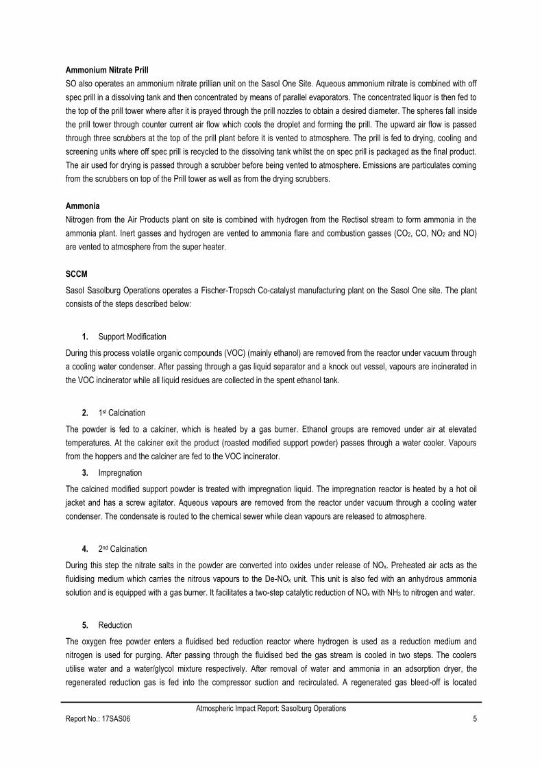
4.2 Point Source Maximum Emission Rates during Normal Operating Conditions .................................................... 24
4.3 Point Source Maximum Emission Rates during Start-up, Maintenance and/or Shut-down .................................. 27
4.4 Fugitive Emissions ................................................................................................................................................ 28
4.4.1 Fallout Dust ...................................................................................................................................................... 28
4.4.2 Fugitive VOCs .................................................................................................................................................. 28
4.5 Emergency Incidents ............................................................................................................................................ 28
5 Impact of Enterprise on the Receiving Environment ...................................................................................................... 30
5.1 Analysis of Emissions’ Impact on Human Health ................................................................................................. 30
5.1.1 Study Methodology .......................................................................................................................................... 30
5.1.2 Legal Requirements ......................................................................................................................................... 37
5.1.3 Regulations Regarding Air Dispersion Modelling ............................................................................................ 38
5.1.4 Atmospheric Dispersion Processes ................................................................................................................. 40
5.1.5 Atmospheric Dispersion Potential .................................................................................................................... 52
5.1.6 Model Performance ......................................................................................................................................... 84
5.1.7 Scenario Emission Inventory ......................................................................................................................... 100
5.1.8 Model Results ................................................................................................................................................ 102
5.1.9 Uncertainty of Modelled Results .................................................................................................................... 135
5.2 Analysis of Emissions’ Impact on the Environment ............................................................................................ 136
5.2.1 Critical Levels for Vegetation ......................................................................................................................... 136
5.2.2 Dustfall ........................................................................................................................................................... 140
Atmospheric Impact Report: Sasolburg Operations
Report No.: 17SAS06 v
5.2.3 Corrosion ....................................................................................................................................................... 142
5.2.4 Sulfur and Nitrogen Deposition Impacts ........................................................................................................ 147
6 Complaints ................................................................................................................................................................... 149
7 Current or planned air quality management interventions............................................................................................ 150
8 Compliance and Enforcement Actions ......................................................................................................................... 151
9 Additional Information................................................................................................................................................... 152
10 Annexure A................................................................................................................................................................... 154
11 Annexure B................................................................................................................................................................... 155
12 References ................................................................................................................................................................... 156
APPENDIX A: Competencies for Performing Air Dispersion Modelling ................................................................................. 159
APPENDIX B: Comparison of Study Approach with the Regulations Prescribing The Format Of The Atmospheric Impact
Report and the Regulations regarding Air Dispersion Modelling (Gazette No 37804 published 11 July 2014) ..................... 161
APPENDIX C: Raw Materials, Abatement Equipment, Atmospheric Emissions and Measured Dustfall at Sasol’s Sasolburg
Operations ............................................................................................................................................................................. 164
APPENDIX D: CALMET Model Control Options .................................................................................................................... 194
APPENDIX E: CALPUFF Model Control Options .................................................................................................................. 196
APPENDIX F: The NO2/NOx Conversion Ratios for NO2 Formation ...................................................................................... 199
APPENDIX G: Time Series Plots for the Measured Ambient Air Quality in the Study Area .................................................. 203
APPENDIX H: Predicted Baseline and Observed Air Concentrations ................................................................................... 210
APPENDIX I: Management of Uncertainties .......................................................................................................................... 214
APPENDIX J: Guidance Note on treatment of uncertainties ................................................................................................. 220
APPENDIX K: Sensitive Receptors included in the Dispersion Model Simulations ............................................................... 222
APPENDIX L: WRF Model Setup .......................................................................................................................................... 223

Atmospheric Impact Report: Sasolburg Operations
Report No.: 17SAS06 vi
List of Tables
Table 1-1: Enterprise details ...................................................................................................................................................... 1
Table 1-2: Contact details of responsible person....................................................................................................................... 1
Table 1-3: Location and extent of the plant ................................................................................................................................ 2
Table 2-1: Listed activities ......................................................................................................................................................... 3
Table 2-2: Unit processes at Sasol Sasolburg ......................................................................................................................... 10
Table 3-1: Raw materials used in the listed activities seeking MES postponement ................................................................ 18
Table 3-2: Appliances and abatement equipment control technology ..................................................................................... 19
Table 4-1: Point source parameters ......................................................................................................................................... 21
Table 4-2: Point source emission rates during normal operating conditions (units: g/s) .......................................................... 24
Table 5-1: Summary description of CALPUFF/CALMET model suite with versions used in the investigation ........................ 36
Table 5-2: National Ambient Air Quality Standards ................................................................................................................. 37
Table 5-3: Acceptable dustfall rates ......................................................................................................................................... 38
Table 5-4: Definition of vegetation cover for different developments (US EPA 2005) ............................................................. 42
Table 5-5: Benchmarks for WRF Model Evaluation ................................................................................................................. 46
Table 5-6: Daily evaluation results for the WRF simulations for the 2015-2017 extracted at OR Tambo(a) ............................. 46
Table 5-7: Meteorological parameters provided for the Sasol monitoring stations in the Sasolburg area ............................... 48
Table 5-8: Daily evaluation results for the WRF simulations for the 2015-2017 extracted at Eco Park(a) ................................ 49
Table 5-9: Parameters of buildings on the SO facility included in the dispersion modelling .................................................... 52
Table 5-10: Monthly temperature summary (2015 - 2017) ...................................................................................................... 55
Table 5-11: Summary of the ambient NH3 measurements at Fence Line for the period 2010-2012 (units: µg/m3) ................ 58
Table 5-12: Summary of the ambient measurements at Leitrim for the period 2015-2017 (units: µg/m3) ............................... 58
Table 5-13: Summary of the ambient measurements at AJ Jacobs for the period 2015-2017 (units: µg/m3) ......................... 59
Table 5-14: Summary of the ambient measurements at Eco Park for the period 2015-2017 (units: µg/m3) ........................... 59
Table 5-15: Summary of the ambient measurements at Three Rivers for the period 2015-2017 (units: µg/m3) ..................... 60
Table 5-16: Summary of the ambient measurements at Sharpeville for the period 2015-2017 (units: µg/m3) ........................ 61
Table 5-17: Summary of the ambient measurements at Zamdela for the period 2015-2017 (units: µg/m3) ............................ 62
Table 5-18: Comparison of predicted and observed SO2 concentrations at monitoring station in Sasolburg ......................... 96
Table 5-19: Comparison of predicted and observed NO2 concentrations at monitoring stations in Sasolburg ....................... 98
Table 5-20: Varying source emissions per scenario provided for SO (units: g/s) .................................................................. 101
Table 5-21: Receptors identified for assessment of impact as a result of SO emissions ...................................................... 103
Table 5-22: Simulated baseline hourly SO2 concentrations and the theoretical change in concentrations relative to the
baseline at the AQMs and 20 closest receptors .................................................................................................................... 106
Table 5-23: Simulated baseline daily SO2 concentrations and the theoretical change in concentrations relative to the
baseline at the AQMs and 20 closest receptors .................................................................................................................... 107
Table 5-24: Simulated baseline annual SO2 concentrations and the theoretical change in concentrations relative to the
baseline at the AQMs and 20 closest receptors .................................................................................................................... 108
Table 5-25: Simulated baseline hourly NO2 concentrations and the theoretical change in concentrations relative to the
baseline at the AQMs and 20 closest receptors .................................................................................................................... 115
Table 5-26: Simulated baseline annual NO2 concentrations and the theoretical change in concentrations relative to the
baseline at the AQMs and 20 closest receptors .................................................................................................................... 116
Table 5-27: Simulated baseline daily PM concentrations and the theoretical change in concentrations relative to the baseline
at the AQMs and 20 closest receptors ................................................................................................................................... 122
Atmospheric Impact Report: Sasolburg Operations
Report No.: 17SAS06 vii
Table 5-28: Simulated baseline annual PM concentrations and the theoretical change in concentrations relative to the
baseline at the AQMs and 20 closest receptors .................................................................................................................... 123
Table 5-29: Simulated baseline hourly CO concentrations and the theoretical change in concentrations relative to the
baseline at the AQMs and 20 closest receptors .................................................................................................................... 129
Table 5-30: Most stringent health-effect screening level identified for all non-criteria pollutants assessed ........................... 131
Table 5-31: Screening of non-criteria pollutants against health risk guidelines ..................................................................... 133
Table 5-32: Proposed unit risk factors for pollutants of interest in the current assessment ................................................... 134
Table 5-33: Excess Lifetime Cancer Risk (New York Department of Health) ........................................................................ 135
Table 5-34: Critical levels for SO2 and NO2 by vegetation type (CLRTAP, 2015) ................................................................. 136
Table 5-35: Summary of dustfall deposition rates as a result of operations at SO ................................................................ 140
Table 5-36: ISO 9223 Classification of the Time of Wetness ................................................................................................ 143
Table 5-37: ISO 9223 classification of pollution by sulfur-containing substances represented by SO2 ................................. 144
Table 5-38: ISO 9223 classification of pollution by sulfur-containing substances represented by SO2 as a result of SO ..... 144
Table 5-39: ISO 9223 classification of pollution by airborne chloride containing substances ................................................ 144
Table 5-40: ISO 9223 classification of pollution by airborne chloride containing substances for SO .................................... 145
Table 5-41: Estimated corrosivity categories of the atmosphere ........................................................................................... 145
Table 5-42: Estimated corrosivity categories of the atmosphere associated with SO ........................................................... 145
Table 5-43: Average and steady state corrosion rates for Different Metals and Corrosivity Categories ............................... 146
Table 5-44: ISOCORRAG regression model constants (Knotkova et al., 1995) .................................................................... 146
Table 5-45: Corrosion rate of metals associated with SO calculated according to the ISOCORRAG method ...................... 147

Atmospheric Impact Report: Sasolburg Operations
Report No.: 17SAS06 viii
List of Figures
Figure 4-1: Locality map of SO in relation to surrounding residential and industrial areas ...................................................... 20
Figure 5-1: The basic study methodology followed for the assessment .................................................................................. 33
Figure 5-2: Schematic displaying how the dispersion modelling scenarios are presented, for each monitoring station receptor
in the modelling domain ........................................................................................................................................................... 35
Figure 5-3: Plume buoyancy .................................................................................................................................................... 42
Figure 5-4: Period, day- and night-time wind rose for OR Tambo for the period 2015 - 2017 ................................................. 47
Figure 5-5: Period, day- and night-time wind rose for WRF data as extracted at OR Tambo for the period 2015 - 2017 ....... 47
Figure 5-6: Monthly temperature profile for WRF data as extracted at OR Tambo and measured data from OR Tambo
SAWS station data for the period 2015 – 2017 ........................................................................................................................ 48
Figure 5-7: CALMET Layer 1 wind vector plot for 15 May 2015 at 05:00 ................................................................................ 49
Figure 5-8: CALMET Layer 1 wind vector plot for 2 February 2016 at 05:00 .......................................................................... 50
Figure 5-9: Land use categories, terrain contours, meteorological WRF grid points and surface station locations displayed on
200 x 200 km CALMET domain (1 km resolution) ................................................................................................................... 51
Figure 5-10: Period, day- and night-time wind rose for Eco Park for the period 2015 - 2017 .................................................. 54
Figure 5-11: Period, day- and night-time wind rose for AJ Jacobs for the period 2015 - 2017 ................................................ 54
Figure 5-12: Period, day- and night-time wind rose for Leitrim for the period 2015 - 2017 ...................................................... 55
Figure 5-13: Monthly average temperature profile for Eco Park (2015 – 2017) ....................................................................... 56
Figure 5-14: Monthly average temperature profile for Leitrim (2015 – 2017) .......................................................................... 56
Figure 5-15: Diurnal atmospheric stability (extracted from CALMET at the Eco Park monitoring point) ................................. 57
Figure 5-16: Observed hourly average SO2 concentrations at Leitrim .................................................................................... 63
Figure 5-17: Observed hourly average SO2 concentrations at AJ Jacobs ............................................................................... 63
Figure 5-18: Observed hourly average SO2 concentrations at Eco Park ................................................................................. 64
Figure 5-19: Observed hourly average SO2 concentrations at Three Rivers ........................................................................... 64
Figure 5-20: Observed hourly average SO2 concentrations at Sharpeville ............................................................................. 65
Figure 5-21: Observed hourly average SO2 concentrations at Zamdela ................................................................................. 65
Figure 5-22: Observed daily average SO2 concentrations at Leitrim ....................................................................................... 66
Figure 5-23: Observed daily average SO2 concentrations at AJ Jacobs ................................................................................. 66
Figure 5-24: Observed daily average SO2 concentrations at Eco Park ................................................................................... 67
Figure 5-25: Observed daily average SO2 concentrations at Three Rivers ............................................................................. 67
Figure 5-26: Observed daily average SO2 concentrations at Sharpeville ................................................................................ 68
Figure 5-27: Observed daily average SO2 concentrations at Zamdela .................................................................................... 68
Figure 5-28: Observed hourly average NO2 concentrations at Leitrim .................................................................................... 69
Figure 5-29: Observed hourly average NO2 concentrations at AJ Jacobs............................................................................... 69
Figure 5-30: Observed hourly average NO2 concentrations at Eco Park ................................................................................ 70
Figure 5-31: Observed hourly average NO2 concentrations at Three Rivers .......................................................................... 70
Figure 5-32: Observed hourly average NO2 concentrations at Sharpeville ............................................................................. 71
Figure 5-33: Observed hourly average NO2 concentrations at Zamdela ................................................................................. 71
Figure 5-34: Observed daily average PM10 concentrations at Leitrim ..................................................................................... 72
Figure 5-35: Observed daily average PM10 concentrations at AJ Jacobs ................................................................................ 72
Figure 5-36: Observed daily average PM10 concentrations at Eco Park .................................................................................. 73
Figure 5-37: Observed daily average PM10 concentrations at Three Rivers ............................................................................ 73
Figure 5-38: Observed daily average PM10 concentrations at Sharpeville .............................................................................. 74
Figure 5-39: Observed daily average PM10 concentrations at Zamdela .................................................................................. 74

Atmospheric Impact Report: Sasolburg Operations
Report No.: 17SAS06 ix
Figure 5-40: Time variation plot of observed SO2 and NO2 concentrations at Leitrim (shaded area indicates 95th percentile
confidence interval) .................................................................................................................................................................. 76
Figure 5-41: Time variation plot of observed SO2 and NO2 concentrations at AJ Jacobs (shaded area indicates 95th
percentile confidence interval) ................................................................................................................................................. 77
Figure 5-42: Time variation plot of observed SO2 and NO2 concentrations at Eco Park (shaded area indicates 95th percentile
confidence interval) .................................................................................................................................................................. 78
Figure 5-43: Time variation plot of observed SO2 and NO2 concentrations at Three Rivers (shaded area indicates 95th
percentile confidence interval) ................................................................................................................................................. 79
Figure 5-44: Time variation plot of observed SO2 and NO2 concentrations at Sharpeville (shaded area indicates 95th
percentile confidence interval) ................................................................................................................................................. 80
Figure 5-45: Time variation plot of observed SO2 and NO2 concentrations at Zamdela (shaded area indicates 95th percentile
confidence interval) .................................................................................................................................................................. 81
Figure 5-46: Time variation plot of normalised observed PM10 and PM2.5 concentrations at Leitrim ....................................... 82
Figure 5-47: Time variation plot of normalised observed PM10 and PM2.5 concentrations at AJ Jacobs ................................. 82
Figure 5-48: Time variation plot of normalised observed PM10 and PM2.5 concentrations at Eco Park ................................... 82
Figure 5-49: Time variation plot of normalised observed PM10 and PM2.5 concentrations at Three Rivers ............................. 83
Figure 5-50: Time variation plot of normalised observed PM10 and PM2.5 concentrations at Sharpeville ................................ 83
Figure 5-51: Time variation plot of normalised observed PM10 and PM2.5 concentrations at Zamdela .................................... 83
Figure 5-52: Polar plot of hourly median SO2 concentration observations at Leitrim for 2015 to 2017 ................................... 86
Figure 5-53: Polar plot of hourly median SO2 concentration observations at AJ Jacobs for 2015 to 2017 ............................. 86
Figure 5-54: Polar plot of hourly median SO2 concentration observations at Eco Park for 2015 to 2017 ............................... 87
Figure 5-55: Polar plot of hourly median SO2 concentration observations at Three Rivers for 2015 to 2017.......................... 87
Figure 5-56: Polar plot of hourly median SO2 concentration observations at Sharpeville for 2015 to 2017 ............................ 88
Figure 5-57: Polar plot of hourly median SO2 concentration observations at Zamdela for 2015 to 2017 ................................ 88
Figure 5-58: Polar plot of hourly median NO2 concentration observations at Leitrim for 2015 to 2017 ................................... 89
Figure 5-59: Polar plot of hourly median NO2 concentration observations at AJ Jacobs for 2015 to 2017 ............................. 89
Figure 5-60: Polar plot of hourly median NO2 concentration observations at Eco Park for 2015 to 2017 ............................... 90
Figure 5-61: Polar plot of hourly median NO2 concentration observations at Three Rivers for 2015 to 2017 ......................... 90
Figure 5-62: Polar plot of hourly median NO2 concentration observations at Sharpeville for 2015 to 2017 ............................ 91
Figure 5-63: Polar plot of hourly median NO2 concentration observations at Zamdela for 2015 to 2017 ................................ 91
Figure 5-64: Polar plot of hourly median PM10 concentration observations at Leitrim for 2015 to 2017 .................................. 92
Figure 5-65: Polar plot of hourly median PM10 concentration observations at AJ Jacobs for 2015 to 2017 ............................ 92
Figure 5-66: Polar plot of hourly median PM10 concentration observations at Eco Park for 2015 to 2017 .............................. 93
Figure 5-67: Polar plot of hourly median PM10 concentration observations at Three Rivers for 2015 to 2017 ........................ 93
Figure 5-68: Polar plot of hourly median PM10 concentration observations at Sharpeville for 2015 to 2017 ........................... 94
Figure 5-69: Polar plot of hourly median PM10 concentration observations at Zamdela for 2015 to 2017 ............................... 94
Figure 5-70: Fractional bias of means and standard deviation for SO2 ................................................................................... 97
Figure 5-71: Fractional bias of means and standard deviation for NO2 ................................................................................... 99
Figure 5-72: Sensitive receptors identified for assessment of impact as a result of Sasol Operations, Sasolburg ............... 102
Figure 5-73: Simulated hourly SO2 concentrations (99th percentile) at AQMS for Sasolburg Operations ............................ 104
Figure 5-74: Simulated daily SO2 concentrations (99th percentile) at AQMS for Sasolburg Operations ............................... 105
Figure 5-75: Simulated annual SO2 concentrations at AQMS for Sasolburg Operations ...................................................... 105
Figure 5-76: Simulated hourly SO2 concentrations (99th percentile) as a result of baseline emissions ................................. 109
Figure 5-77: Simulated hourly SO2 concentrations (99th percentile) as a result of theoretical compliance with new plant
emission standards ................................................................................................................................................................ 109
Figure 5-78: Simulated hourly SO2 concentrations (99th percentile) as a result of alternative emissions .............................. 110
Figure 5-79: Simulated daily SO2 concentrations (99th percentile) as a result of baseline emissions ................................... 110

Atmospheric Impact Report: Sasolburg Operations
Report No.: 17SAS06 x
Figure 5-80: Simulated daily SO2 concentrations (99th percentile) as a result of theoretical compliance with new plant
emission standards ................................................................................................................................................................ 111
Figure 5-81: Simulated daily SO2 concentrations (99th percentile) as a result of alternative emissions ................................ 111
Figure 5-82: Simulated annual SO2 concentrations as a result of baseline emissions .......................................................... 112
Figure 5-83: Simulated annual SO2 concentrations as a result of theoretical compliance with new plant emission standards
............................................................................................................................................................................................... 112
Figure 5-84: Simulated annual SO2 concentrations as a result of alternative emissions ....................................................... 113
Figure 5-85: Simulated hourly NO2 concentrations (99th percentile) at AQMS for Sasolburg Operations ............................. 114
Figure 5-86: Simulated annual NO2 concentrations at AQMS for Sasolburg Operations ...................................................... 114
Figure 5-87: Simulated hourly NO2 concentrations (99th percentile) as a result of baseline emissions ................................. 117
Figure 5-88: Simulated hourly NO2 concentrations (99th percentile) as a result of theoretical compliance with new plant
emission standards ................................................................................................................................................................ 117
Figure 5-89: Simulated hourly NO2 concentrations (99th percentile) as a result of alternative emissions .............................. 118
Figure 5-90: Simulated annual NO2 concentrations as a result of baseline emissions .......................................................... 118
Figure 5-91: Simulated annual NO2 concentrations as a result of theoretical compliance with new plant emission standards
............................................................................................................................................................................................... 119
Figure 5-92: Simulated annual NO2 concentrations as a result of alternative emissions ...................................................... 119
Figure 5-93: Simulated daily PM concentrations (99th percentile) at AQMS for Sasolburg Operations ................................. 121
Figure 5-94: Simulated annual PM concentrations at AQMS for Sasolburg Operations ....................................................... 121
Figure 5-95: Simulated daily PM concentrations (99th percentile) as a result of baseline emissions .................................... 124
Figure 5-96: Simulated daily PM concentrations (99th percentile) as a result of theoretical compliance with new plant
emission standards ................................................................................................................................................................ 124
Figure 5-97: Simulated daily PM concentrations (99th percentile) as a result of alternative emissions ................................. 125
Figure 5-98: Simulated annual PM concentrations as a result of baseline emissions ........................................................... 125
Figure 5-99: Simulated annual PM concentrations as a result of theoretical compliance with new plant emission standards
............................................................................................................................................................................................... 126
Figure 5-100: Simulated annual PM concentrations as a result of alternative emissions ...................................................... 126
Figure 5-101: Simulated hourly CO concentrations (99th percentile) at AQMS for Sasolburg Operations ............................ 127
Figure 5-102: Observed hourly CO concentrations (99th percentile) at AQMS for Sasolburg Operations ............................. 128
Figure 5-103: Simulated hourly CO concentrations (99th percentile) as a result of baseline emissions ................................ 130
Figure 5-104: Simulated hourly CO concentrations (99th percentile) as a result of theoretical compliance with new plant
emission standards ................................................................................................................................................................ 130
Figure 5-105: Simulated hourly CO concentrations (99th percentile) as a result of alternative emissions ............................ 131
Figure 5-106: Simulated annual Mn concentrations as a result of baseline emissions ......................................................... 134
Figure 5-107: Annual SO2 concentrations as a result of baseline emissions compared with CLRTAP critical levels............ 137
Figure 5-108: Annual SO2 concentrations as a result of theoretical compliance with new plant emission standards compared
with CLRTAP critical levels .................................................................................................................................................... 137
Figure 5-109: Annual SO2 concentrations as a result of alternative emissions compared with CLRTAP critical levels ........ 138
Figure 5-110: Annual NO2 concentrations as a result of baseline emissions compared with CLRTAP critical levels ........... 138
Figure 5-111: Annual NO2 concentrations as a result of theoretical compliance with new plant emission standards compared
with CLRTAP critical levels .................................................................................................................................................... 139
Figure 5-112: Annual NO2 concentrations as a result of alternative emissions compared with CLRTAP critical levels ........ 139
Figure 5-113: Simulated daily dustfall as a result of baseline emissions ............................................................................... 140
Figure 5-114: Simulated daily dustfall as a result of theoretical compliance with new plant standards ................................. 141
Figure 5-115: Simulated daily dustfall as a result of alternative emissions ............................................................................ 141

Atmospheric Impact Report: Sasolburg Operations
Report No.: 17SAS06 xi
Abbreviations
AAA Acrylic acid and acrylate
AEL Atmospheric Emission Licence
AIR Atmospheric Impact Report
AQA Air quality act
AQMS Air quality monitoring stations
As Arsenic
ATR Auto Thermal Reformer
APCS Air pollution control systems
ARM Ambient Ratio Method
ASG Atmospheric Studies Group
BPIP Building Profile Input Program
CH4 Methane
Cl2 Chlorine
Co Cobalt
CO Carbon monoxide
CO2 Carbon dioxide
Cr Chromium
Cu Copper
DEA Department of Environmental Affairs
EDC 1,2-dichloroethane
g Gram
g/s Gram per second
HCl Hydrogen chloride
HCN Hydrogen cyanide
HNO3 Nitric acid
H2 Hydrogen
H2O Water
H2S Hydrogen Sulfide
HSP High Sulfur Pitch
IP Intellectual property
IPCC Intergovernmental Panel on Climate Change
kV Kilo volt
LMo Monin-Obukhov length
m Meter
m² Meter squared
m³ Meter cubed
MES Minimum Emission Standards
MIBK Methyl isobutyl ketone
Mn Manganese
m/s Meters per second
N2 Nitrogen
NAAQS National Ambient Air Quality Standards (as a combination of the NAAQ Limit and the allowable frequency
of exceedance)
NaCN Sodium cyanide

Atmospheric Impact Report: Sasolburg Operations
Report No.: 17SAS06 xii
NaOH Sodium hydroxide
NAP Nirtic Acid Plant
NEMA National Environmental Management Act
NEMAQA National Environmental Management Air Quality Act
NH3 Ammonia
Ni Nickel
NO Nitrogen oxide
NO2 Nitrogen dioxide
NOx Oxides of nitrogen
O3 Ozone
OH Hydroxyles
OLM Ozone Limiting Method
PBL Planetary boundary layer
Pb Lead
PM Particulate matter
PM10 Particulate matter with diameter of less than 10 µm
PM2.5 Particulate matter with diameter of less than 2.5 µm
ppb Parts per billion
PVC Polyvinyl chloride
RNO3 Organic nitrates
Sb Antimony
SO2 Sulfur dioxide (1)
SO3 Sulfur trioxide (1)
SO4 Sulfates
SOx Oxides of sulfur (1)
SSBR Sasol Slurry Bed Reactor
TEOS Tetraethyl Orthosilcate
US EPA United States Environmental Protection Agency
USGS United States Geological Survey
V Vanadium
VOC Volatile organic compound
WRF The Weather Research and Forecasting Mesoscale Model
yr Year
Zo Roughness length
µ micro
°C Degrees Celsius
Note:
(1) The spelling of “sulfur” has been standardised to the American spelling throughout the report. "The International Union of Pure
and Applied Chemistry, the international professional organisation of chemists that operates under the umbrella of UNESCO,
published, in 1990, a list of standard names for all chemical elements. It was decided that element 16 should be spelled
“sulfur”. This compromise was to ensure that in future searchable data bases would not be complicated by spelling variants.
(IUPAC. Compendium of Chemical Terminology, 2nd ed. (the "Gold Book"). Compiled by A. D. McNaught and A. Wilkinson.
Blackwell Scientific Publications, Oxford (1997). XML on-line corrected version: http://goldbook.iupac.org (2006) created by M.
Nic, J. Jirat, B. Kosata; updates compiled by A. Jenkins. ISBN 0-9678550-9-8.doi: 10.1351/goldbook)"

Atmospheric Impact Report: Sasolburg Operations
Report No.: 17SAS06 xiii
Glossary
Advection Transport of pollutants by the wind
Airshed An area, bounded by topographical features, within which airborne contaminants can be retained for an extended period
Algorithm A mathematical process or set of rules used for calculation or problem-solving, which is usually undertaken by a computer
Alternative Emission Limit Ceiling or maximum emission limit requested by Sasol, with which it commits to comply
Assessment of environmental effects A piece of expert advice submitted to regulators to support a claim that adverse effects will or will not occur as a result of an action, and usually developed in accordance with section 88 of the Resource Management Act 1991
Atmospheric chemistry The chemical changes that gases and particulates undergo after they are discharged from a source
Atmospheric dispersion model A mathematical representation of the physics governing the dispersion of pollutants in the atmosphere
Atmospheric stability A measure of the propensity for vertical motion in the atmosphere
Building wakes Strong turbulence and downward mixing caused by a negative pressure zone on the lee side of a building
Calm / stagnation A period when wind speeds of less than 0.5 m/s persist
Cartesian grid A co-ordinate system whose axes are straight lines intersecting at right angles
Causality The relationship between cause and effect
Complex terrain Terrain that contains features that cause deviations in direction and turbulence from larger-scale wind flows
Configuring a model Setting the parameters within a model to perform the desired task
Convection Vertical movement of air generated by surface heating
Convective boundary layer The layer of the atmosphere containing convective air movements
Data assimilation The use of observations to improve model results – commonly carried out in meteorological modelling
Default setting The standard (sometimes recommended) operating value of a model parameter
Diagnostic wind model (DWM) A model that extrapolates a limited amount of current wind data to a 3-D grid for the current time. It is the ‘now’ aspect, and makes the model ‘diagnostic’.
Diffusion Clean air mixing with contaminated air through the process of molecular motion. Diffusion is a very slow process compared to turbulent mixing.
Dispersion The lowering of the concentration of pollutants by the combined processes of advection and diffusion
Dispersion coefficients Variables that describe the lateral and vertical spread of a plume or a puff
Dry deposition Removal of pollutants by deposition on the surface. Many different processes (including gravity) cause this effect.
Sasolburg Operations (SO) Sasol South Africa (Pty) Limited operating through its Sasolburg Operations,
Atmospheric Impact Report: Sasolburg Operations
Report No.: 17SAS06 1
Atmospheric Impact Report: Sasol Sasolburg Operations
1 ENTERPRISE DETAILS
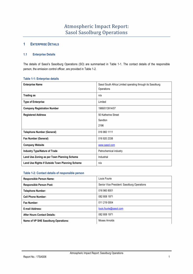
1.1 Enterprise Details
The details of Sasol’s Sasolburg Operations (SO) are summarised in Table 1-1. The contact details of the responsible
person, the emission control officer, are provided in Table 1-2.
Table 1-1: Enterprise details
Enterprise Name Sasol South Africa Limited operating through its Sasolburg
Operations
Trading as n/a
Type of Enterprise Limited
Company Registration Number 1968/013914/07
Registered Address 50 Katherine Street
Sandton
2196
Telephone Number (General) 016 960 1111
Fax Number (General) 016 920 2338
Company Website www.sasol.com
Industry Type/Nature of Trade Petrochemical industry
Land Use Zoning as per Town Planning Scheme Industrial
Land Use Rights if Outside Town Planning Scheme n/a
Table 1-2: Contact details of responsible person
Responsible Person Name: Louis Fourie
Responsible Person Post: Senior Vice President: Sasolburg Operations
Telephone Number: 016 960 8001
Cell Phone Number: 082 808 1971
Fax Number: 011 219 0004
E-mail Address: [email protected]
After Hours Contact Details: 082 808 1971
Name of VP SHE Sasolburg Operations: Moses Arnolds
Atmospheric Impact Report: Sasolburg Operations
Report No.: 17SAS06 2
1.2 Location and Extent of the Plant
Table 1-3: Location and extent of the plant
Physical Address of the Plant Sasol 1 Site
1 Klasie Havenga Street
Sasolburg
1947
Description of Site (Where no Street Address) Subdivision 6 of 2 of Driefontein No- 2 and certain subdivisions of the farm Saltberry Plain, Roseberry Plain Flerewarde and Antrim and subdivision 5 of 4 of Montrose, District of Sasolburg, Free State.
Coordinates of Approximate Centre of Operations Sasol 1 Site:
Latitude: S 26.82678 Longitude: E 27.84206
Extent 15.51 km2
Elevation Above Sea Level 1 498 m
Province Free State
Metropolitan/District Municipality Fezile Dabi District Municipality
Local Municipality Metsimaholo
Designated Priority Area Vaal Triangle Priority Area
1.3 Atmospheric Emission Licence and other Authorisations
The following authorisations, permits and licences related to air quality management are applicable:
• Atmospheric Emission License:
o FDDM-MET-2013-18
o FDDM-MET-2013-20
o FDDM-MET-2013-22
o FDDM-MET-2013-23-P2
o FDDM-MET-2013-24
• Other: None

Atmospheric Impact Report: Sasolburg Operations
Report No.: 17SAS06 3
2 NATURE OF THE PROCESS
2.1 Listed Activities
A summary of listed activities currently undertaken at SO is provided in Table 2-1.
Table 2-1: Listed activities
Category
of Listed
Activity
Subcategory
of listed
activity
Listed activity name Description of the Listed Activity
1 1.1
Solid Fuel Combustion
installations
Solid fuels (excluding biomass) combustion installations used primarily
for steam raising or electricity generation
1.5 Reciprocating Engines Liquid and gas fuel stationary engines used for electricity generation
2
2.1 Petroleum Industry Petroleum industry, the production of gaseous and liquid fuels as well
as petrochemicals from crude oil, coal, gas or biomass
2.4
Petroleum Industry (Storage
and handling of petroleum
products
All permanent immobile liquid storage facility on a single site with a
combined storage capacity of greater than 1000 m3
6 6.1 Organic Chemical Industry
The production, or use in production, of organic chemicals not specified
elsewhere including acetylene, ecetic, maleic or phthalic anhydride or
their acids, carbon disulphide, pyridine, formaldehyde, acetaldehyde,
acrolein and its derivatives, acrylonitrile, amines and synthetic rubber.
The production of organometallic compounds, organic dyes and
pigments, surface-active agents.
The polymerisation or co-polymerisation of any unsaturated
hydrocarbons, substituted hydrocarbon (including Vinyl chloride).
The manufacture, recovery or purification of acrylic acid or any ester of
acrylic acid.
The use of toluene di-isocyanate or other di-isocyanate of comparable
volatility; or recovery of pyridine.
All permanent immobile liquid storage facilities at a single site with a
combined storage capacity of greater than 1 000 m3.
7
7.1
Inorganic chemicals industry
The use of ammonia in the manufacturing of ammonia
7.2 The primary production of nitric acid in concentrations exceeding 10%
7.3 The manufacturing of ammonium nitrate and its processing into
fertilisers
7.4
Manufacturing activity involving the production, use or recovery of
antimony, beryllium, cadmium, chromium, cobalt, lead, mercury,
selenium, thalium and their salts
7.7 Production of Caustic Soda Production of Caustic Soda
8 8.1
Thermal treatment of
hazardous and general
waste
Facilities where general and hazardous waste are treated by the
application of heat (Applicable : Capacity of Incinerator > 10 kg/hour)

Atmospheric Impact Report: Sasolburg Operations
Report No.: 17SAS06 4
2.2 Process Description
A description on the process units operating at SO is provided below.
Steam Stations
SO operates two steam/power stations. Pulverised coal is fired in boilers which are used for steam and power generation.
All the steam and the majority of the power generated at these stations are used for Sasol’s purposes, however Sasol do
supply Eskom with electricity directly into the national grid to alleviate the pressure on the national grid, for which Steam
Station 1 is critical. Emissions include combustion gases; sulfur dioxide (SO2), nitrogen oxide (NO), nitrogen dioxide (NO2),
particulate matter (PM), carbon dioxide (CO2) and carbon monoxide (CO).
Auto Thermal Reformers
SO operates two Auto Thermal Reformers (ATRs) on the Sasol One facility. Natural gas is reformed in the ATRs to form the
building blocks of the Fischer Tropsch process. The heat required in the ATRs is obtained from the Fired Heaters which is
fired with process tail gas, except during startup when they are fired with natural gas. Emissions from the two Fired Heaters
are combustion gas products, such as NO, NO2, CO and CO2. No sulfur compounds are present.
Rectisol
SO operates a Rectisol plant on the Sasol One Site. The purpose of the Rectisol plant is “dew point correction” and “CO2”
removal. Due to the high concentration of methane and other hydrocarbons, the gas from the first two stages are sent to the
flare and those from the last three stages are sent to atmosphere through the Steam Station 1 Stacks. Emissions include
hydrocarbons specifically with high concentrations of CO2 emitted from the Steam Station 1 stacks.
Thermal Oxidation
SO operates a thermal oxidation unit where various waste streams from various plants are thermally oxidized. The thermal
oxidation facility consists of three incinerators, namely: the B6993, B6990 and B6930 incinerators. As part of the oxidation
process, heat is recovered by means of steam, which supplements the steam supply to the plants from the Steam Stations.
The B6930 incinerator has a bag house for particulate emission control, whilst the B6993 incinerator has a caustic scrubber
for both SO2 and PM emission control.
Benfield
SO operates a Benfield unit as part of the ammonia plant on the Sasol One Site. The Benfield unit consists of a CO2
absorber column were CO2 is removed from the process gas stream using the benfield solution. The benfield solution is
regenerated in the desorber column were the CO2 is desorbed to the atmosphere.
Nitric acid plant (NAP)
A nitric acid plant is operational at the Sasol Bunsen Street site. Ammonia is piped from the cold storage area to the nitric
acid plant where it is reacted with oxygen to produce oxides of nitrogen (NOx), as an intermediate product, which is fed to a
catalyst to selectively convert NO to NO2. The NO2 is fed to a series of absorption columns where nitric acid is formed. The
exhaust vent from the second tower, which contains NO2, and N2O is sent to the de-NOx reactor, where the gas is reduced
over a catalyst to nitrogen and oxygen, which is released to atmosphere.
Ammonium Nitrate solution
SO operates an ammonium nitrate solution plant. This plant is integrated into the NAP plant. The nitric acid from the NAP
plant is reacted with ammonia in a reactor to form the ammonium nitrate solution.
Atmospheric Impact Report: Sasolburg Operations
Report No.: 17SAS06 5
Ammonium Nitrate Prill
SO also operates an ammonium nitrate prillian unit on the Sasol One Site. Aqueous ammonium nitrate is combined with off
spec prill in a dissolving tank and then concentrated by means of parallel evaporators. The concentrated liquor is then fed to
the top of the prill tower where after it is prayed through the prill nozzles to obtain a desired diameter. The spheres fall inside
the prill tower through counter current air flow which cools the droplet and forming the prill. The upward air flow is passed
through three scrubbers at the top of the prill plant before it is vented to atmosphere. The prill is fed to drying, cooling and
screening units where off spec prill is recycled to the dissolving tank whilst the on spec prill is packaged as the final product.
The air used for drying is passed through a scrubber before being vented to atmosphere. Emissions are particulates coming
from the scrubbers on top of the Prill tower as well as from the drying scrubbers.
Ammonia
Nitrogen from the Air Products plant on site is combined with hydrogen from the Rectisol stream to form ammonia in the
ammonia plant. Inert gasses and hydrogen are vented to ammonia flare and combustion gasses (CO2, CO, NO2 and NO)
are vented to atmosphere from the super heater.
SCCM
Sasol Sasolburg Operations operates a Fischer-Tropsch Co-catalyst manufacturing plant on the Sasol One site. The plant
consists of the steps described below:
1. Support Modification
During this process volatile organic compounds (VOC) (mainly ethanol) are removed from the reactor under vacuum through
a cooling water condenser. After passing through a gas liquid separator and a knock out vessel, vapours are incinerated in
the VOC incinerator while all liquid residues are collected in the spent ethanol tank.
2. 1st Calcination
The powder is fed to a calciner, which is heated by a gas burner. Ethanol groups are removed under air at elevated
temperatures. At the calciner exit the product (roasted modified support powder) passes through a water cooler. Vapours
from the hoppers and the calciner are fed to the VOC incinerator.
3. Impregnation
The calcined modified support powder is treated with impregnation liquid. The impregnation reactor is heated by a hot oil
jacket and has a screw agitator. Aqueous vapours are removed from the reactor under vacuum through a cooling water
condenser. The condensate is routed to the chemical sewer while clean vapours are released to atmosphere.
4. 2nd Calcination
During this step the nitrate salts in the powder are converted into oxides under release of NOx. Preheated air acts as the
fluidising medium which carries the nitrous vapours to the De-NOx unit. This unit is also fed with an anhydrous ammonia
solution and is equipped with a gas burner. It facilitates a two-step catalytic reduction of NOx with NH3 to nitrogen and water.
5. Reduction
The oxygen free powder enters a fluidised bed reduction reactor where hydrogen is used as a reduction medium and
nitrogen is used for purging. After passing through the fluidised bed the gas stream is cooled in two steps. The coolers
utilise water and a water/glycol mixture respectively. After removal of water and ammonia in an adsorption dryer, the
regenerated reduction gas is fed into the compressor suction and recirculated. A regenerated gas bleed-off is located

Atmospheric Impact Report: Sasolburg Operations
Report No.: 17SAS06 6
between the water cooler and water glycol chiller. Water and ammonia removed from the gas is routed to the chemical
sewer.
6. Coating
The active catalyst requires coating to prevent auto-ignition. This is done by feeding the catalyst into the coating tank where
it is suspended in molten wax (synthetic paraffins). Wax volatiles from the wax melt tank and coating tank are routed to a
separate dedicated wax scrubber where they are stripped with water. Stripper water from the wax melt tank scrubber is
routed to the storm water drain, while stripper water from the coating tank scrubber is routed to the chemical sewer as it may
contain metals. Clean gas from both scrubbers is released to atmosphere. Both tanks and transfer lines have jackets with
hot oil for heating.
7. Packaging
Finished product (active catalyst suspended in wax) runs through to the drum filling station using a nitrogen purge, to
package the product for distribution and use.
Phenol, Cresol and TNPE Plants
The Phenol, cresol and TNPE plants extract and purifies a range of phenolic products from tar acid containing feed streams
sourced from Sasol Synfuels Operations. Various process chemicals are used to extract the tar acids and to remove
impurities where-after phenol, cresols and xylenols are recovered via distillation. Waste generated by the processes are
either incinerated or treated at the Sasol Bio-works. All relieve valves and vents are connected to the plant’s flare system
and normal combustion products are emitted (CO2, CO, NO, NO2 and water (H2O)). The fuel gas furnace emits combustion
gas products and SO2 and sulfur trioxide (SO3) are emitted from the oxides of sulfur (SOX) scrubber.
Solvents
All vents and hydrocarbon emissions from Solvents are sent to the flare with the exception of a few units which vent
hydrocarbons to atmosphere which has been quantified.
Methanol High Purity
Gas and hydrogen is reacted in a synthesis reactor at Sasol Waxes where crude methanol is produced. The distillation of
the crude methanol into high purity methanol takes place at Sasol Solvents, through atmospheric distillation. The purification
is accomplished through degassing and the removal of low and high boiling point by-products.
Methanol Technical Grade
The methanol extracted from the reaction water (Chemical water treatment plant) is purified to methanol technical grade
through a process of atmospheric distillation. The purification is accomplished through the removal of low and high boiling
point by-products.
Chemical Water Recovery
Chemicals are recovered from the reaction water from the Sasol Waxes synthesis processes, as well as purge streams from
Butanol and by-products from HP methanol, TG methanol, MIBK and FTDR. Recovery of chemicals takes place through a
process of atmospheric distillation and degassing.

Atmospheric Impact Report: Sasolburg Operations
Report No.: 17SAS06 7
Methyl Iso Butyl Ketone (MIBK 1 and 2)
DMK (acetone) is converted over a palladium impregnated resin ion-exchange catalyst in the presence of hydrogen to MIBK
via a single stage process. The reactor product is worked up and purified through a series of distillation columns. All
impurities and co-products are removed through the distillation processes.
Solvents Blending Plant
Raw material from Secunda, Sasolburg and outside suppliers, transported via road tankers to the blending plant, are stored
in on-site storage tanks. The raw products, mixed according to customers specifications, are supplied to the customer via
road tankers or drums.
Heavy Alcohol Plant
Raw material from Secunda (Sabutol bottoms) is distilled through a single step distillation column into 2 final products, i.e.
pentylol and hexylol. No by-products are removed in the process.
Solvents Mining Chemicals Plant
Raw material from Secunda, Sasolburg and outside suppliers, transported via road tankers to the blending plant, are stored
in on-site storage tanks. The raw products, mixed according to customers specifications, are supplied to the customer via
road tankers or drums.
AAA/Butanol
Sasol operates an Acrylic Acid and Acrylate (AAA) as well as a Butanol plant on the Sasol Midland Site.
Butanol
Synthesis gas is fed to a cold box separation phase where impurities are removed from the syngas. The impurities are
recycled back into the gas loop and vented into an elevated flare. The purified syngas as well as propylene are fed into a
series of reactive distillation units to produce n-butanol and i-butanol as the final product. All columns are vented to the flare.
AAA
Acrylic acid is manufactured by reacting propylene with air through a series of reactors and a distillation / purification
process. The crude Acrylic Acid is fed to three processes. It can be purified to form Glacial Acrylic Acid, it can be reacted
with n-Butanol to produce Butyl Acrylate or it can be reacted with Ethanol to produce Ethyl Acrylate. All vents from the AAA
plant goes through high temperature incinerator to eliminate any Acrylates entering the atmosphere, especially due to the
odorous nature of Ethyl Acrylate. Off gasses from the catalytic destruction unit and the vapour combustion unit contains
CO2, CO, NO and NO2.
LOC
Liquid bulk storage contains/stores the various products produced on site. It is coupled to the loading bay which is covered
to the vapour combustion. Drum, road and rail loading takes place. The fugitive organic vapour emitted during loading of
road bulk haul trucks are extracted from the tanker hoods and incinerated at the vapour combustion unit. Emissions are
normal combustion gasses such as CO2, CO and H2O. No sulfur components are present.
Ethylene
Sasol, Sasolburg Chemical Operations operates a Monomer production and separation unit where ethylene is produced to
be used within the polyethylene and polyvinylchloride manufacturing plants. A Mixture of ethane and ethylene is piped to
Sasolburg from Secunda where it enters the Ethylene Purification Unit (S4500) where the ethylene is separated from the
ethane by means of distillation. The ethylene is then routed to the customers.

Atmospheric Impact Report: Sasolburg Operations
Report No.: 17SAS06 8
The ethane product from the S4500 is then routed to the Cracking Unit (S4600) where it is cracked to ethylene. Once
cracked, the ethylene/ethane gas mixture goes through a quenching, scrubbing and drying phase where after the gas is
selectively hydrogenated to convert acetylene to ethylene. After this the C2 mixture is purified by means of distillation
processes where light and heavy components as well as unreacted ethane are removed. The ethylene is then stored in the
ethylene tank to be distributed to the polythene and vinyl chloride monomer plants. Hydrocarbon off-gasses are sent to the
plant’s main flare where it is converted to CO2, CO and H2O. The cracking unit emits traces of H2S from the caustic
scrubber.
Polyethylene
SO operates two polyethylene plants on the Sasol Midland Site, namely the Poly 2 and Poly 3 plants.
Poly 2: The Poly 2 process involves the manufacture of linear low density polyethylene in a fluidized bed gas phase reactor.
The materials used for the manufacture comprise ethylene which is the main component, hexene/butene as a density
modifier, hydrogen as a melt index modifier, isopentane for temperature control, a silica based Ziegler Natta catalyst
(manufacture in house in the catalyst plant, a catalyst activator and nitrogen for reactor pressure control. The feeds enter the
reactor where the reaction process takes place and polymer together with some unreacted gas is transferred to the
degassing bin for separation of hydrocarbons from the polymer. The liquid hydrocarbons (hexene, isopentane) is recovered
in the monomer recovery section of the plant and recycled back to the reactor for re-use. The polymer pneumatically
transferred from the degassing bin and is stored in intermediate storage silos and thereafter pelletised at the extruder. At the
extruder, virgin polymer is mixed with additives, is melted and is thereafter cut it into pellets in an underwater cutter. This
polymer pellets are thereafter dried and cooled before being pneumatically conveyed to the Pack Silos from which it is
bagged at the packline and stored in the warehouse. Emergency venting occurs through the plant flare system where
ethylene is converted to CO2, CO and H2O.
Poly 3: The Poly 3 plant produces medium and low density polyethylene. The ethylene is fed to a reactor where initiator and
modifier depending on which grade (LDPE or MDPE) is added and the polymerization reaction take place. The excess
ethylene is recycled and the polyethylene is separated, extruded, dried and transferred to degassing silos where the access
ethylene is purged out with air. After degassing the product is transferred for packaging. Emergency venting occurs through
the plant flare system where ethylene is converted to CO2, CO and H2O.
Chlorine
Sasol also operates a chlorine, hydrochloric acid, sodium hydroxide and sodium hypochlorite production facility on the Sasol
Midlands Site. Salt is conveyed to a dissolving tank where the salt is dissolved up to a specific brine concentration. After
several purification steps, the brine solution is fed to the chloro-caustic cells where chlorine, hydrogen and aqueous sodium
hydroxide is manufactured. The chlorine manufactured is stored, reacted with sodium hydroxide to create sodium
hypochlorite or reacted with hydrogen to create hydrochloric acid in the hydrogen chloride (HCl) burners. The hydrogen is
either used at the HCl burners to manufacture HCl or sent to the VCM plant as a fuel gas. The hydrochloric acid produced in
the HCl burners is stored and sold as a final product. Scrubbers and outlets might contain traces of HCl and chlorine (Cl2).
Vinyl Chloride Monomer
Sasol operates a Vinyl Chloride Monomer (VCM) production facility on the Sasol Midland Site. The facility uses two different
reactions for the manufacturing of the intermediate 1,2-dichloroethane (EDC). The first is the direct chlorination of ethylene
to produce EDC. The second is the oxychlorination step where ethylene, oxygen, hydrogen and HCl react to produce crude
EDC and water. The water is separated after the oxychlorination reactor and the crude EDC is sent to the EDC purification
unit. The water stream is fed to the water recovery unit for purification before being exported to the Sasol Polymers Chlorine
Plant for brine make up. EDC from the purification step is fed to the EDC cracker together with EDC from the direct

Atmospheric Impact Report: Sasolburg Operations
Report No.: 17SAS06 9
chlorination step. In the EDC cracking unit EDC is cracked to VCM and HCl after which the cracked stream is fed to the
VCM purification unit. Here the VCM and HCl are separated and HCl is recycled to the oxychlorination unit. The VCM is sent
to storage in two spheres at the PVC Plant. By products from the EDC Purification Unit and plant vent gasses are
incinerated and the recovered dilute hydrochloric acid exported to the Sasol Polymers Hydrochloric Acid Plant.
Polyvinyl Chloride
Sasol operates a Polyvinyl chloride plant on the Sasol Midland Site. VCM from the VCM plant storage spheres is suspended
in water whilst the reaction is brought up to the desired temperature. The polymerization reaction takes place and the
polyvinyl chloride (PVC) is formed. The reactor is discharged into a blow down vessel which feeds into the stripper, where
unreacted VCM is recovered from the slurry and recycled. The PVC/water mixture is then fed to the slurry stock tank and
then to the centrifuge where the PVC is separated. Once the PVC is separated, it is dried, screened and pneumatically fed
to the storage area for packaging. The unreacted VCM is recovered by liquefaction and stored for reuse. The
uncompressible tail gas from the latter unit is fed to the incinerator at the VCM Plant.
Cyanide
Sasol, furthermore, operates a Cyanide manufacturing plant on the Sasol Midland Site. Methane (CH4) rich natural gas
reacts with NH3 in a fluidized coke bed reactor to form a hydrogen cyanide (HCN) rich synthesis gas. The energy required
for the endothermic reactor is supply by a set of six graphite electrode connected to a 6.6kV electrical supply. The synthesis
gas and large coke particles leaving the reactor are transferred through a cyclone where the particles are separated from
the gas. After the cyclone, the gas is cooled and fed to fabric filters where any carbon soot entrained in the synthesis gas is
removed. The “polished” gas is then fed to a pair of sodium hydroxide (NaOH) absorbers installed in series. Here the HCN
reacts with the NaOH to form sodium cyanide (NaCN), which is the final product. The exhaust gasses from the second
NaOH absorber is fed into a NaOH vent scrubber after which it is emitted to atmosphere via an elevated stack. Emissions
contain mainly hydrogen, particulates from the bag houses and are measured for traces of HCN.
Wax
Sasol Wax operates a catalyst preparation plant as well as two wax production units namely the Sasol Slurry Bed Reactors
(SSBR) and the Arge Reactors. In the catalyst preparation plant metals are dissolved in nitric acid and then precipitated
after which the catalyst is dried and activated, where after it is ready for use. NOx is emitted at one and particulates are
emitted at three stacks in the area.
The three SSBRs and Arge reactors are fed with the active catalyst and synthesis gas to produce hydrocarbons. The
hydrocarbons are worked up via hydrogenation, distillation and oxidation to liquid final products. The products are blended,
solidified and packed. Organics and combustion gasses (CO2, CO, H2O, NO and NO2) are emitted from various heaters
within the process. Hydrocarbons from vents are sent to the factory main flare system where the organics are converted to
CO2, CO and H2O before being emitted to atmosphere
2.3 Unit Processes
All unit processes for the SO complex are listed in Table 2-2. The listed activity for which the postponement is applied is
indicated as bold text. Sasol’s Sasolburg Operations also operates various activities including water treatment facilities, fine
ash dams, research activities and various distillation and processing units that are not included in the Listed Activities and
Minimum Emissions Standards (MES). The site is a gas plant and as such continuous emissions are limited to
predominantly combustion gases where flares have been installed as safety mechanisms.

Atmospheric Impact Report: Sasolburg Operations
Report No.: 17SAS06 10
Table 2-2: Unit processes at Sasol Sasolburg
Unit Process Function of Unit Process Batch or Continuous
Process
ATR
Auto Thermal reformers Convert natural gas to reform gas Continuous
Membrane separators Purification of reformed gas Continuous
Flares Destruction of gas Batch
Rectisol CO2 removal and dew point correction Continuous
Thermal oxidation
B6993 Spent Caustic Incinerator The incineration of spent caustic solution and off specification solvent products including MIBK by-products in a down fired incinerator.
Continuous
Spent Caustic Storage - F6903 Intermediate storage Batch
Hydrocarbon Solvents - F6963 A/B F6927 B Intermediate storage Batch
Sodium Carbonate - F6954 Intermediate storage Batch
Caustic - F6959 / F6975 Intermediate storage Batch
B6930 High Sulfur Pitch Incinerator The incineration of High Sulfur Pitch, Organic solvents and High Organic waters in a limestone fluidized bed unit.
Continuous
HSP Storage tanks - F6926 / F6990 Intermediate storage Batch
HOW tank - F6938 Intermediate storage Batch
BFW tank - F6939 Intermediate storage Batch
B6990 Chemical Incinerator The incineration of heavy oils, off-specification waxes, Sasol spent catalyst, funda filter cake, slop solvents and high organic waste.
Continuous
Product tank Intermediate storage Batch
Steam Stations
Fuel oil tanks Holding fuel Continuous
Coal bunkers/silos Holding coal Continuous
15 Boilers Steam production Continuous
Feed water tanks Holding water Continuous
Resins (HCL, caustic) Holding chemicals Continuous
NH3 tank Holding ammonia Continuous
Blow down tank Continuous
Nitric Acid (NAP)
NO reactor Reaction of NH3 and air to form NO Continuous
Absorber columns Absorbtion of NO2 to HNO3 Continuous
De-NOx reactor Reduction of NOx to O2 and N2 Continuous
Ammonium Nitrate
AN reactor Reaction to form ammonium nitrate Continuous
Neutralizer pH correction Continuous
AN solution tank Storage of AN solution Continuous
Prillan
Wet section Concentration of ammonium NH4OH solution Continuous

Atmospheric Impact Report: Sasolburg Operations
Report No.: 17SAS06 11
Unit Process Function of Unit Process Batch or Continuous
Process
Dry section Drying of prilled NH4OH Continuous
Storage Storage of prilled NH4OH Continuous
Ammonia
CO2 capture Remove moisture from the CO2 stream Continuous
CO-shift Reacts CO + steam to form H2 Continuous
Benfield Removal of CO2 from the process stream Continuous
PSA Production of LPH2 Continuous
Deoxo N2 purification Continuous
Ammonia synthesis Production of NH3 Continuous
BFW Demineralized water Continuous
SCCM
Storage tanks/bags Containing raw materials for the support
modification step
Continuous
Reactor Allow for chemical reactions Batch
VOC destruction unit Destroying VOC vapours Continuous
Hoppers Temporary storage of the support powder Continuous
Water cooler Cooling the roasted support powder for storage Continuous
Mixing tank Mixing cobalt nitrate, water and metal promoter Batch
Heated reactor Impregnating support powder with the metals and
subsequent partial drying
Batch
DeNOx unit Catalytic destruction of NOx fumes Continuous
Sieve Sizing of the particles Continuous
Reverse pulse jet cartridge filters Removing of dust particulates Continuous
Purge hopper Remove oxygen Continuous
Reduction reactor Activation step on the catalyst Continuous
Coolers Cooling of the activated catalyst Continuous
Wax CoatingTank Wax coating of the activated catalyst Continuous
Packaging unit Package of the activated catalyst for distribution Continuous
Vent System Removing of dust particles from step 1,4,6 and 7
hoppers off gas.
Continuous
Phenol, Cresol and TNPE
Phenol producing column Process NBF DTA material for phenol production Continuous
Feedstock storage Hold feed material Batch
Rundown tanks Hold product phenol Batch
Final product tanks Hold final product phenol Batch
Product Stabiliser tanks Hold chemicals Batch
Tempered water system Hold and provide condensate to phenol unit Continuous

Atmospheric Impact Report: Sasolburg Operations
Report No.: 17SAS06 12
Unit Process Function of Unit Process Batch or Continuous
Process
Relief system Relief system in high pressure cases Batch
HP steam Provide heat to phenol unit reboilers/heater Continuous
HOW Storage tanks Holding high organic effluent materials Batch
Sand Filtration Filter solids from HOW water Continuous
Extraction Extract phenolics from the high organic wastewater Continuous
C stream distillation Recover butyl acetate (solvent) Continuous
Stripping section Strip out butyl acetate from final effluent Continuous
Crude tar acids storage Hold tar acids extracted from high organic effluent Batch
Separators Remove tar and oil from high organic stream Continuous
Storage tanks Holding raw materials – Formalin, Caustic Soda, O-cresol, Water
Batch
Atmospheric and Vacuum Dehydration
Removal of water from crude resin by heating
Batch Stripping of unreacted o-cresol from crude resin by direct steam injection under vacuum conditions
Pastillising Pastillising of resin to form final product Batch
Buffer storage Intermediate storage of resin before pastillsing Batch
Feed storage tanks Holding raw materials as buffer between Secunda and Sasolburg
Batch
Drying and N-base removal Removing excess water from the feed followed by a process step to remove unwanted nitrogen base compounds from the feed
Continuous
Phenol production Phenol produced from cleaned-up cresol feed Continuous
Phenol removal Remaining phenol in bottom product from above unit has to be removed
Continuous
Product Splitter Separates cresol products from feed based on boiling points differences
Continuous
Intermediate feed product storage Between units products are temporarily stored to minimize the whole production train to be affected if one unit experiences problems
Batch / Continuous
Final product tanks Bulk storage before shipment to customer Batch / Continuous
Loading facility Road tanker loading of intermediate or final products
Batch
Loading facility Road tanker loading of pitch type material for transport to incineration plant
Batch
Solvents – All plants
Off-loading facility Off-loading raw material to holding tank Batch
Loading Facilities Loading final product Batch
Final product tanks Holding product Batch
Solvents – AAA/Butanol
Oxidation Raw material to crude product Continuous
Distillation Purification of crude product Continuous
Esterification Reaction of crude product with specific alcohol Continuous
Refrigeration unit - NH3 Cooling in process Continuous
Cryogenic separation Conditioning of synthesis gas Continuous
Chemical Dosing In-process requirement Continuous
Flare system Process gas Continuous

Atmospheric Impact Report: Sasolburg Operations
Report No.: 17SAS06 13
Unit Process Function of Unit Process Batch or Continuous
Process
Off gas incineration Incineration of process and tank waste gas Continuous
Catalytic combustion VOC combustion Continuous
Solvents – MIBK 1 and 2
Raw material tank Holding raw materials Continuous
Compression Preparation of raw material Continuous
High pressure Reaction Production of raw product Continuous
Refrigeration Unit Preparation of vapour (H2) emissions to flare Continuous
Distillation Fractionation of product to desired spec. Continuous
Prover tanks Stores MIBK while being analysed before being pumped to final storage tank Batch
Catalyst Loading Facilities Loading and washing of catalyst for D551 A&B Batch
Solvents – Methanol
Synthesis Converting gas and hydrogen to crude methanol Continuous
Raw crude methanol tank Holding raw materials Continuous
Prover product tanks Holding product Batch
Atmospheric distillation Distill methanol from crude Continuous
Caustic dozing Corrosion control and neutralization of acids Continuous
Solvents – Methanol TG
Atmospheric distillation Distill methanol in reaction water to Technical grade purity
Continuous
Prover tanks Storage of Methanol TG Continuous
Solvents – E1204
Prover tanks Holding product Continuous
Atmospheric distillation Distill Pentylol and Hexylol from Sabutol Bottoms Continuous
Solvents – Chemical Recovery (S500) Alcohol distillation
Degassing Dissolved gases are removed from chemical water Continuous
Feed storage Reaction water Storage to E501 Continuous
Atmospheric distillation Removal of water and other light components from chemical water
Continuous
Scrubbing Vapours are scrubbed of acids Continuous
Solvents – Blending plant
Raw material Feed for blends Batch
Blending tanks To blend formulations according to customer requirements
Batch
Storage Final Products Batch
Solvents – Mining Chemicals plant
Raw material Feed for blends Batch
Blending tanks To blend formulations according to customer requirements
Batch
Storage Final Products Batch
Vapour combustion unit Destruction of organic vapours from the loading racks Batch
Various storage tanks Storage of liquid products Continuous

Atmospheric Impact Report: Sasolburg Operations
Report No.: 17SAS06 14
Unit Process Function of Unit Process Batch or Continuous
Process
Poly 2
Feed Streams:
Knock-out drum Knock out oil entrainment in supply ethylene Continuous
Ethylene Compression Compression of supply ethylene from supply pressure to reaction pressure
Continuous
Hydrogen Storage Acceptance of supply high pressure hydrogen from air products line
Continuous
Raw material offloading Offloading of rail cars / isocontainers into storage tanks before use in catalyst and LLDPE manufacturing
Batch
Catalyst Plant:
Dehydration Preparation of silica for use in the manufacture of catalyst
Batch
Catalyst Preparation Manufacture of Ziegler Natta, silica based catalyst for the polyethylene manufacture process
Batch
Catalyst Storage Storage of catalyst manufactured and transfer to reactor catalyst feeders
Batch
Catalyst Deactivation Deactivation of out of specification catalyst Batch
Purification Purification of feed streams to remove trace poisons before use in the Catalyst and LLDPE manufacturing processes
Continuous and batch
Reaction Produce polyethylene in the fluidized bed reactor Continuous
Degassing:
Degassing Bin Degassing of reactor polymer to remove hydrocarbons from polymer and screen polymer to prevent conveying line blockages
Continuous
Monomer recovery Knock out hydrocarbons from degassing bin vent via a compressor and fridge system – recycle liquid hydrocarbons to the reactor
Continuous
Flare
Flaring of hydrocarbons not recovered at the monomer recovery unit
Continuous
Flaring of reactor inventory during reactor shutdown / purging
- Batch
Blending:
Intermediate storage Intermediate storage and feed of reactor polymer to the extruder
Batch
Extruder Mixing of reactor polymer with additives and pelletising
Batch
Packline Bagging of polymer into 25kg bags and 1.25ton semi bulk bags
Batch
Warehouse Storage of polymer before being transported to customers
Batch
Poly 3
Ethylene Feed
Knock-out drum Knock-out oils and wax formation in feed line Continuous
Compressors Compress Ethylene to required reaction pressure Continuous
Reactor Produce Polyethylene Continuous
Separators Separate Ethylene from Polyethylene Continuous
Recycle unit
Knock-out drums Knock-out oils and wax formation Continuous
Heat exchangers Cool down ethylene Continuous
Off-loading Area

Atmospheric Impact Report: Sasolburg Operations
Report No.: 17SAS06 15
Unit Process Function of Unit Process Batch or Continuous
Process
Buffer Tank Isododecane used as flushing agent Batch
Buffer Tank Compressor Lubrication Oil (Polybutene & Polyglycol)
Batch
Storage tank (iso-tanker) Contain Propionaldehyde used as modifier solvent Batch
Extrusion Pelletise polymer Continuous
Pellet transfer and degassing Transfer pellets and degas product Continuous
Waste oil and initiator Disposal of waste oil and initiator Batch
Flare system Flaring ethylene or propylene Batch
VCM and PVC
Reactor VCM Plant Unit 1100 – manufacture of 1,2-dichloroethane (EDC) from ethylene and chlorine.
Continuous
Cracker VCM Plant Unit 1400 – cracking of EDC to form vinyl chloride monomer (VCM) and hydrogen chloride (HCl)
Continuous
Reactor VCM Plant Unit 1200 – manufacture of EDC by oxyhydrochlorination of ethylene
Continuous
Incinerator VCM Plant Unit 1600 – by-product hydrochloric acid recovery from mixed gaseous and liquid plant streams from both the VCM and PVC Plants.
Continuous
Scrubber VCM Plant Unit 1500 Safety Scrubber – removal of HCl from gaseous vent streams during incinerator off-line time.
Batch
Cold flare
VCM Plant Unit 1500 Cold Flare – vent gaseous streams of VCM and HCl diluted with steam and nitrogen during emergencies and gas clearing in preparation for maintenance shutdown.
Batch
Tanks – spheres PVC Plant Storage Spheres – storage of VCM Continuous / Batch
Reactors PVC Plant Reaction Unit – manufacture of poly (vinyl chloride) (PVC) from VCM
Batch
Separation - recovery PVC Plant Vinyl Chloride Recovery Unit – recovery of unreacted VCM from the manufacture of PVC
Continuous
Drying PVC Plant Drying Unit – remove moisture from raw PVC polymer
Continuous
Separation - recovery PVC Plant Multigrade Recovery Unit – recovers PVC polymer from effluent water streams
Batch
Monomers
Ethylene unit 4600 Cracking of ethane and propane Separation of ethylene & ethane from C2 rich gas
Continuous
Ethylene storage tank Storage of final product Continuous
Ethane storage sphere Storage of furnace feed material Continuous
Propylene storage sphere and bullets Storage of final product Continuous
Cracker system Cracking of ethane or propane to ethylene (This unit operation include boiler feed water, dilution steam, crack gas quench, MEA, Caustic and fuelgas)
Continuous
Cooling water system Used as cooling medium Continuous
Loading bay facility Loading of ethylene road tanker Batch
Feed gas preparation Ethane saturator Continuous
Compression Crack gas compression as well as ethylene and propylene compression
Continuous
Flare system Flaring of off-spec product during upset conditions as well as over-pressure protection (3 flares: Ground flare; elevated flare and tank flare)
Continuous
Cold separation This unit operation include de-ethaniser, C3-recovery, secondary feed gas drying, cold
Continuous

Atmospheric Impact Report: Sasolburg Operations
Report No.: 17SAS06 16
Unit Process Function of Unit Process Batch or Continuous
Process
separation, de-methaniser, ethylene cycle, C2-splitter and ethane system
Liquefaction This unit operation include propylene refrigeration, ethylene distribution and storage
Batch
Pre-cooling and drying Propylene system, pre-cooling, acetylene removal, primary feed gas drying
Continuous
Utilities
Plant air, instrument air, LP nitrogen, de-oxo nitrogen, fire steam, 38bar HP steam, 4.5bar MP steam & 1.5bar LP steam, drinking water, condensate & fire water system
Continuous / Batch
DCS system Digital Control System for plant operation Continuous
Cyanide
Water Process make up water Batch
Nitrogen Plant purging, bag house pulsing and coke feed Continuous
Caustic Diluted caustic for the production of sodium cyanide Batch
Ammonia For the production of hydrogen cyanide gas Continuous
Sodium cyanide Primary and secondary absorption Batch
Sodium cyanide Crude Tanks Batch
Sodium cyanide Final storage Batch
Natural gas Piped in for the production of hydrogen cyanide gas Continuous
Bag house Filtering of hydrogen cyanide gas Continuous
Absorbers Absorbing HCN gas into caustic Continuous
Back up scrubbers Final separation of HCN gas from waste gas stream Continuous
Stack and seal pot Exhausting waste gas mainly hydrogen into atmosphere
Continuous
Press filter Filtration of crude sodium cyanide Batch
Nash compressors Recycle hydrogen system into process When required
Loading facility Dispatch of final product Continuous
Chlorine
Chlorine production To produce chlorine, hydrogen, sodium hydroxide Continuous
Calcium Chloride Produce calcium chloride Batch
Hydrochloric Acid Hydrochloric acid Continuous
Tank farm Storage and dispatch of caustic soda, hydrochloric acid and sulfuric acid.
Continuous
Sasol Wax – Production
Reactors Production of hydrocarbons Continuous
Distillation column Separation of hydrocarbons Continuous
Packaging Solidification of wax to get required products Continuous
Bagging Packaging of products Continuous
Mixing and blending Production of catalyst Batch
Hoppers Storage of sodium carbonate Batch
Sasol Wax – Catalyst preparation
Dissolving reactors To produce a metal solution Batch
Precipitation reactors To precipitate the catalyst slurry from precursor solutions
Batch

Atmospheric Impact Report: Sasolburg Operations
Report No.: 17SAS06 17
Unit Process Function of Unit Process Batch or Continuous
Process
Calcination To strengthen the catalyst particles Continuous
Driers To dry the catalyst to the correct moisture content Continuous
Evaporators To concentrate the by-product solution from the precipitation area
Continuous
Crystallisers To crystallise a salt slurry solution Continuous
Drier To dry the salt crystals Continuous
Storage tanks Storage for nitric acid, potassium silicate, and caustic soda.
Batch

Atmospheric Impact Report: Sasolburg Operations
Report No.: 17SAS06 18
3 TECHNICAL INFORMATION
Raw material consumption for the listed activities applying for MES postponement at SO is tabulated in Table 3-1. For
completeness, the raw materials used by all process are included in Appendix C1 (Table C-1), unless the information is
intellectual property (IP) or otherwise sensitive due to competition law. Pollution abatement technologies employed at SO for
the listed activities applying for MES postponement are provided in Table 3-2 (all appliance and abatement equipment in
use at SO is provided in Appendix C; Table C-2).
3.1 Raw Materials Used and Production Rates
Table 3-1: Raw materials used in the listed activities seeking MES postponement
Raw Material Type Design Consumption Rate
(Volume) Units (quantity/period)
Thermal oxidation
Spent Caustic 30 660 t/a
Organic Solvents 13 140 t/a
High Sulfur Pitch 21 900 t/a
Organic Solvents 17 520 t/a
Limestone 26 280 t/a
Organic waste water 17 520 t/a
Off- specification waxes 720 t/a
Sasol spent catalyst 2 448 t/a
Funda filter cake 2 640 t/a
Polyethylene wax 960 t/a
Other solid waste 1 800 t/a
High organic waste 4 800 t/a
Pitch/ tar waste
Slops oils 1 800 t/a
Fuel Gas 8 760 kNm3/a
Steam Station 1 and 2
Water (Steam Station 1) 6 132 kt/a
Water (Steam Station 2) 9 070 kt/a
Coal (Steam Station 1) 2 148 kt/a
Coal (Steam Station 2) 2 000 kt/a

Atmospheric Impact Report: Sasolburg Operations
Report No.: 17SAS06 19
3.2 Appliances and Abatement Equipment Control Technology
Table 3-2: Appliances and abatement equipment control technology
Appliance name Appliance type/description Appliance function/purpose
Spent Caustic Incinerator B6993
Scrubber Venturi scrubber Scrubbing of flue gasses to remove
particulates and SO2
New High Sulfur Pitch (HSP) Incinerator B6930
Fluidized bed Limestone fluidized bed Removal of SO2
Bag house Bag house Particulate removal
Steam Station 1 and 2
Electrostatic Precipitators Electrostatic precipitators Reducing the quantity of particulate
emissions from the boilers.

Atmospheric Impact Report: Sasolburg Operations
Report No.: 17SAS06 20
4 ATMOSPHERIC EMISSIONS
The establishment of a comprehensive emission inventory for the listed activities seeking postponement formed the basis
for the assessment of the air quality impacts from SO on the receiving environment.
Point source parameters are provided in Table 4-1. A locality map indicating the position of SO in relation to surrounding
residential and industrial areas is included as Figure 4-1. For completeness, the details for all point sources at SO are
provided in Appendix C1; Table C-3 and Table C-4.
Figure 4-1: Locality map of SO in relation to surrounding residential and industrial areas

Atmospheric Impact Report: Sasolburg Operations
Report No.: 17SAS06 21
4.1 Point Source Parameters
Table 4-1: Point source parameters
Point Source number
Source name Latitude (decimal degrees)
Longitude (decimal degrees)
Height of Release Above
Ground (m)
Height Above Nearby
Building (m) (a)
Diameter at Stack Tip /
Vent Exit (m)
Actual Gas Exit
Temperature (°C)
Actual Gas Volumetric Flow (m³/hr)
Actual Gas Exit Velocity
(m/s)
Continuous or batch
Baseline point sources
I1 AAA: ST6010 -26.8230 27.8680 20 0.95 846 36 923.95 14.47 Continuous
I2 Butanol ST1040 -26.8233 27.8668 25 1.5 123 68 515.78 10.77 Continuous
I60 F501 + F 502 vent 26.7762 27.8447 15 0.16 35 50.67 0.70 Continuous
I61 F 505 vent 26.7762 27.8447 15 0.1 176 57.11 2.02 Continuous
I62 E1204 26.7759 27.8447 15 0.1 24 12.44 0.44 Continuous
I63 B 1102 26.7759 27.8447 10 0.4 59 452.39 1.00 Continuous
I64 F1133 A+B 26.7759 27.8447 15 0.1 27 36.76 1.30 Continuous
I3 Fired Heater ATR A Train -26.8263 27.8406 65 52 3.32 190 460 932 14.79 Continuous
I4 Fired Heater ATR B Train -26.8267 27.8408 65 52 3.32 226 488 669 15.68 Continuous
I65 – I67 Rectisol 26.8227 27.8401 75 5 Combined with Steam Station 1
I5 J 4062 A Dust scrubber -26.8290 27.8410 22 9 1 29 56 181 19.87 Continuous
I6 J 4062 B Dust scrubber -26.8290 27.8410 22 1 28 56 436 19.96 Continuous
I7 J4063 A -26.8290 27.8410 85 1.5 21 232 712 36.58 Continuous
I8 J4063 B -26.8290 27.8410 85 1.5 23 94 599 14.87 Continuous
I9 J4063 C -26.8290 27.8410 85 1.5 23 66 607 10.47 Continuous
I10 Steam cracker furnaces, B002a,b -26.8320 27.8440 20 10 1.8 527 106 175 11.59 Continuous
I11 Steam cracker furnaces, B003 and MEA
-26.8319 27.8440 26 16 1.2 200 34 608 8.5 Continuous
I12 Fuel gas furnace -26.8302 27.8474 40 1.3 384 30 629 6.41 Continuous
I68 Phenol Plant -26.8239 27.8406 30 0.2 29 26 0.23 Continuous
I69 SOx scrubber on N-base units -26.8300 27.8470 12 0.11 101 1 984 58.00 Continuous
I13 Oven B 4701 -26.8308 27.8463 26 1 409 7 804 2.76 Continuous
I14 Oven B 4702 -26.8308 27.8463 26 1 320 7 408 2.62 Continuous
I15 Oven B 4801 -26.8308 27.8464 26 1.25 165 13 960 3.16 Continuous

Atmospheric Impact Report: Sasolburg Operations
Report No.: 17SAS06 22
Point Source number
Source name Latitude (decimal degrees)
Longitude (decimal degrees)
Height of Release Above
Ground (m)
Height Above Nearby
Building (m) (a)
Diameter at Stack Tip /
Vent Exit (m)
Actual Gas Exit
Temperature (°C)
Actual Gas Volumetric Flow (m³/hr)
Actual Gas Exit Velocity
(m/s)
Continuous or batch
I16 Oven B 4802 -26.8308 27.8465 26 1.25 285 7 289 1.65 Continuous
I17 Cat prep SBR -26.8313 27.8426 15 0.5 100 7 166 10.14 Continuous
I18 SCR outlet -26.8294 27.8408 40 On top of roof 1.00 40 16 116 5.70 Continuous
I19 Furnace B2801 -26.8262 27.8429 20 None in the
vicinity 0.7 356 3 879 2.80 Continuous
I20 Furnace B1521 -26.8258 27.8426 20 None in the
vicinity 0.77 336 4 694 2.80 Continuous
I21 Furnace B2471 -26.8316 27.8499 45 None in the
vicinity 0.97 324 6 997 2.63 Continuous
I22 Fired Heater (B2601) 26.4924 27.5031 39.1 n/a 1.40 35 3 547 0.64 Continuous
I27 VCM incinerator -26.8300 27.8730 30 0.36 45 4 104 11.20 Continuous
I28 VCM Cracker -26.8300 27.8730 40 1.71 390 101 693 12.30 Continuous
I29 PVC Dryer stack North (A) -26.8279 27.8733 35 1.8 57 131 917 14.40 Continuous
I30 PVC Dryer stack South (B) -26.8279 27.8734 35 1.8 61 141 352 15.43 Continuous
PVC Multigrade (sludge plant) vent Stack
-26.8276 27.8741 6 0.05 100 89.06 12.60 Continuous
PVC Slurry Stock Tank Stack -26.8272 27.8744 35 1.2 45 61 073 15.00 Continuous
PVC Reaction Stack North -26.8276 27.8741 24 0.60 30 7 736 7.60 Continuous
PVC Reaction Stack South -26.8272 27.8735 24 0.60 30 7 736 7.60 Continuous
I54 DeNOx unit -26.8255 27.8387 30 21.5 0.6 450 12 215 12 Continuous
I55 DeNOx unit -26.8255 27.8387 30 21.5 0.6 450 12 215 12 Continuous
I56 Step 4 burner flue gas -26.8258 27.8385 30 19 0.15 330 636.17 10 Continuous
I57 Step 6 burner flue gas -26.8259 27.8385 30 19 0.15 330 636.17 10 Continuous
I58 Hot oil system fuel gas burner -26.8257 27.8385 27 19 0.3 330 279.92 1.1 Continuous
I59 Step 7 burner flue gas -26.8259 27.8385 29 19 0.3 550 865.19 3.4 Continuous
I35
Bay 1 (stack 1 - 6)
-26.8196 27.8477 27 1.2 200 89 166 21.90 Continuous
I36 -26.8196 27.8477 27 1.2 200 105 981 26.03 Continuous
I37 -26.8196 27.8477 27 1.2 200 121 168 29.76 Continuous
I38 -26.8196 27.8477 27 1.2 200 102 724 25.23 Continuous

Atmospheric Impact Report: Sasolburg Operations
Report No.: 17SAS06 23
Point Source number
Source name Latitude (decimal degrees)
Longitude (decimal degrees)
Height of Release Above
Ground (m)
Height Above Nearby
Building (m) (a)
Diameter at Stack Tip /
Vent Exit (m)
Actual Gas Exit
Temperature (°C)
Actual Gas Volumetric Flow (m³/hr)
Actual Gas Exit Velocity
(m/s)
Continuous or batch
I39 -26.8196 27.8477 27 1.2 200 114 613 28.15 Continuous
I40 -26.8196 27.8477 27 1.2 200 110 378 27.11 Continuous
I41
Bay 2 (stack 7-12)
-26.8194 27.8482 27 1.2 200 111 600 27.41 Continuous
I42 -26.8194 27.8482 27 1.2 200 113 514 27.88 Continuous
I43 -26.8194 27.8482 27 1.2 200 119 539 29.36 Continuous
I44 -26.8194 27.8482 27 1.2 200 118 888 29.20 Continuous
I45 -26.8194 27.8482 27 1.2 200 116 404 28.59 Continuous
I46 -26.8194 27.8482 27 1.2 200 108 383 26.62 Continuous
I47
Bay 3 (stack 13-18)
-26.8192 27.8486 27 1.2 200 66 569 16.35 Continuous
I48 -26.8192 27.8486 27 1.2 200 105 778 25.98 Continuous
I49 -26.8192 27.8486 27 1.2 200 123 122 30.24 Continuous
I50 -26.8192 27.8486 27 1.2 200 65 266 16.03 Continuous
I51 -26.8192 27.8486 27 1.2 200 73 694 18.10 Continuous
I52 -26.8192 27.8486 27 1.2 200 54 232 13.32 Continuous
I53 NAP Bunsen Street -26.8252 27.8602 75 1.5 215 39 634 6.23 Continuous
Point sources applying for postponement
I31 Heavy Ends B incinerator (B6990)
-26.8255 27.8404 40 1.5 650 69 979 11.00 Continuous
I32 High sulfur pitch incinerator (B6930)
-26.8254 27.8402 40 1.5 180 159 043 25.00 Continuous
I33 Spent caustic incinerator (B6993) -26.8255 27.8404 40 1.2 83 60 258 14.80 Continuous
I23 SS1 Boiler 4 -26.8222 27.8407 75 2.5 160 235 030 13.3 Continuous
I24 SS1 Boiler 5&6 -26.8224 27.8404 75 2.5 160 458 751 25.96 Continuous
I25 SS1 Boiler 7&8 -26.8225 27.8401 75 2.5 160 478 543 27.08 Continuous
I26 SS2 Boiler 9-15 -26.8222 27.8488 145 7.8 160 1 746 014 10.15 Continuous
Notes: (a) “Height above nearby building” is given as the minimum difference between the release height and the height of nearby buildings, where the point source is located equidistant from more than one
building. Building height differences only included for sources affected by building downwash effects. (b) Height of release lower than nearby building.

Atmospheric Impact Report: Sasolburg Operations
Report No.: 17SAS06 24
4.2 Point Source Maximum Emission Rates during Normal Operating Conditions
In cases where periodic compliance measurements are conducted, these are measured in accordance with the methods prescribed in Schedule A of the MES and aligned with what is
prescribed in the Atmospheric Emission Licence (AEL). These reflect the average of measurements conducted over a 3-hour period during normal operating conditions.
Table 4-2: Point source emission rates during normal operating conditions (units: g/s)
Point Source number
Industry name Source name SO2 NOX as
NO2 PM CO HF
Sum of heavy metals
Hg Cd+Tl TOCs VOCs
I1
Solvents
AAA: ST6010 0.31 0.04 0.11 9.51E-6
I2 Butanol ST1040 0.05 0.08 0.18 4.44E-1
I60 F501 + F 502 vent 3.90E-1
I61 F 505 vent 5.89E-1
I62 E1204 5.89E-1
I63 B 1102 1.34
I64 F1133 A+B 3.69E-1
I3 ATR Phenosolvan
Fired Heater ATR A Train 0.13 4.19 0.02
I4 Fired Heater ATR B Train 0.19 1.89 0.12
I65 – I67 Rectisol 292.94 0.097
I5
Prillan Plant
J 4062 A Dust scrubber 0.03
I6 J 4062 B Dust scrubber 0.02
I7 J4063 A 0.12
I8 J4063 B 0.06
I9 J4063 C 0.03
I10 Sasol Polymers - Monomers (excluding flares)
Steam cracker furnaces, B002a,b
0.14 0.4306 0.11
I11 Steam cracker furnaces, B003 and MEA
5.71E-3 1.82 8.24E-3
I12
Merisol (excluding flares)
Fuel gas furnace 2.85E-2 0.19 8.24E-3
I68 Phenol Plant 2.03 2.54E-3
I69 SOx scrubber on N-base units
5.93E-3 5.98E-1 6.34E-4
I13 Sasol Wax Oven B 4701 3.49E-3 1.27E-2 1.90E-2
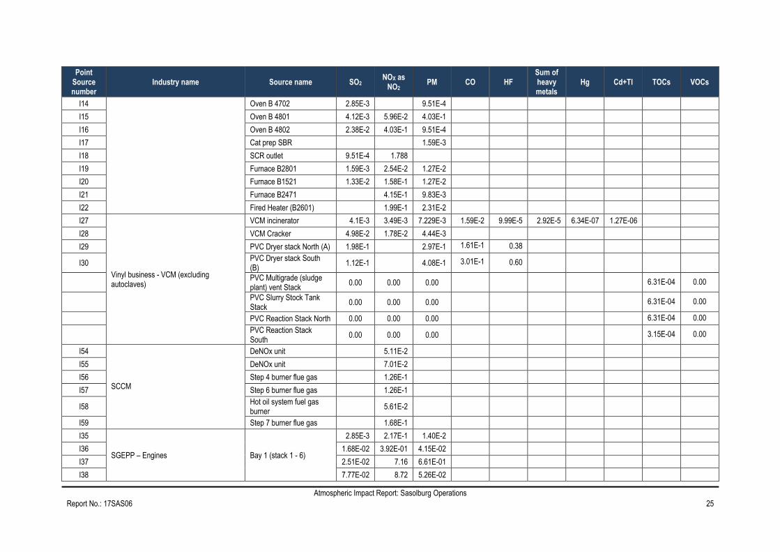
Atmospheric Impact Report: Sasolburg Operations
Report No.: 17SAS06 25
Point Source number
Industry name Source name SO2 NOX as
NO2 PM CO HF
Sum of heavy metals
Hg Cd+Tl TOCs VOCs
I14 Oven B 4702 2.85E-3 9.51E-4
I15 Oven B 4801 4.12E-3 5.96E-2 4.03E-1
I16 Oven B 4802 2.38E-2 4.03E-1 9.51E-4
I17 Cat prep SBR 1.59E-3
I18 SCR outlet 9.51E-4 1.788
I19 Furnace B2801 1.59E-3 2.54E-2 1.27E-2
I20 Furnace B1521 1.33E-2 1.58E-1 1.27E-2
I21 Furnace B2471 4.15E-1 9.83E-3
I22 Fired Heater (B2601) 1.99E-1 2.31E-2
I27
Vinyl business - VCM (excluding autoclaves)
VCM incinerator 4.1E-3 3.49E-3 7.229E-3 1.59E-2 9.99E-5 2.92E-5 6.34E-07 1.27E-06
I28 VCM Cracker 4.98E-2 1.78E-2 4.44E-3
I29 PVC Dryer stack North (A) 1.98E-1 2.97E-1 1.61E-1 0.38
I30 PVC Dryer stack South (B)
1.12E-1 4.08E-1 3.01E-1 0.60
PVC Multigrade (sludge plant) vent Stack
0.00 0.00 0.00 6.31E-04 0.00
PVC Slurry Stock Tank Stack
0.00 0.00 0.00 6.31E-04 0.00
PVC Reaction Stack North 0.00 0.00 0.00 6.31E-04 0.00
PVC Reaction Stack South
0.00 0.00 0.00 3.15E-04 0.00
I54
SCCM
DeNOx unit 5.11E-2
I55 DeNOx unit 7.01E-2
I56 Step 4 burner flue gas 1.26E-1
I57 Step 6 burner flue gas 1.26E-1
I58 Hot oil system fuel gas burner
5.61E-2
I59 Step 7 burner flue gas 1.68E-1
I35
SGEPP – Engines Bay 1 (stack 1 - 6)
2.85E-3 2.17E-1 1.40E-2
I36 1.68E-02 3.92E-01 4.15E-02
I37 2.51E-02 7.16 6.61E-01
I38 7.77E-02 8.72 5.26E-02

Atmospheric Impact Report: Sasolburg Operations
Report No.: 17SAS06 26
Point Source number
Industry name Source name SO2 NOX as
NO2 PM CO HF
Sum of heavy metals
Hg Cd+Tl TOCs VOCs
I39 9.73E-02 6.40 1.33E-01
I40 2.79E-02 7.42E-01 1.42E-01
I41
Bay 2 (stack 7-12)
2.79E-02 4.34 5.55E-02
I42 1.11E-02 3.94E-01 4.15E-02
I43 1.68E-02 3.47E-01 4.15E-02
I44 1.40E-02 3.64E-01 9.16E-02
I45 3.04E-02 1.64E-01 3.04E-02
I46 7.52E-02 3.50E-01 5.83E-02
I47
Bay 3 (stack 13-18)
5.71E-03 6.22 4.39E-01
I48 1.40E-02 3.17 3.90E-02
I49 5.83E-02 1.88 5.83E-02
I50 1.93E-02 3.41 2.22E-02
I51 1.68E-02 2.94 2.79E-02
I52 1.93E-02 1.53 2.51E-02
I53 NAP Bunsen Street NAP Bunsen Street 3.63
I31
Section 6900
Heavy Ends B incinerator (B6990)
2.47 1.34 1.40 0.05 7.77E-03 1.41E-01 3.17E-05 3.17E-05 3.53E-2 1.90E-3
I32 High sulfur pitch incinerator (B6930)
40.68 9.04 1.14 0.11 1.36E-02 6.78E-02 5.07E-04 5.71E-04 1.69E-1
I33 Spent caustic incinerator (B6993)
2.83 4.57 3.27 12.07 6.53E-03 2.2E-01 9.51E-05 3.17E-05 2.17E-01
I23
Steam station
SS1 Boiler 4 30.49 55.27 6.28
I24 SS1 Boiler 5&6 59.51 107.88 12.27
I25 SS1 Boiler 7&8 62.08 112.51 12.81
I26 SS2 Boiler 9-15 226.51 353.91 28.32

Atmospheric Impact Report: Sasolburg Operations
Report No.: 17SAS06 27
4.3 Point Source Maximum Emission Rates during Start-up, Maintenance and/or Shut-down
Unplanned downtime events such as upset conditions are undesirable from a production perspective as well as an
environmental perspective and Sasol endeavours to minimise unplanned downtime by conducting regular and pro-active
maintenance and ensuring control of the process within their designed operating parameters. While unplanned downtime
cannot be completely eliminated, it is minimised as far as practicably possible, and rectified with high priority.
The MES prescribes that start-up, shut-down, upset and maintenance events should not exceed 48-hours – and if they do, a
Section 30 National Environmental Management Act (NEMA) incident is incurred (as also indicated in the Air Emission
Licence (AEL)). SO can confirm that, in the preceding two years, its facility has not exceeded the 48-hour window during
start up, maintenance, upset and shutdown conditions, which has ensured that ambient impacts are limited in duration.
Sasol owns and operates accredited ambient air quality monitoring stations in the vicinity of its Sasolburg plant. The real-
time ambient air quality monitoring data is closely followed during upset conditions at the plant, to ensure that air quality
does not exceed the national ambient air quality standards as a consequence of Sasol’s activities.
SO has an annual phase shut down on both the Sasol One and Midland sites with a total shut-down once every four years
for statutory maintenance and inspections. These shut-downs are planned well in advance. Visible emissions are normally
associated with cold start-up from the Nitric acid plant and boilers as well as the reformers, which results in the flaring of
gas.
The Atmospheric Impact Report (AIR) Regulations require that the maximum emissions during start-up, shut down and
upset conditions must be included within the AIR for the processes. This information is unfortunately not available for two
practical reasons, explained below.
1. Since Sasol operates predominantly gaseous plants, operating the plant under start-up, shut down and upset
condition is a period of high instability and for safety reasons, as few people as possible are allowed on the plant.
Therefore ad hoc sampling under these conditions is a safety risk and therefore the sampling cannot be
conducted. It should further be emphasised that the aim of the plant personnel is to get the plant back into
operation as soon as possible and therefore the support required by sampling teams cannot be provided as the
focus is on returning the plant to stable operation.
Another practical limitation is identification of the precise process conditions that will result in a maximum emission
concentration. Since these conditions are unstable, large variations in plant conditions occur dynamically and pin
pointing the exact combination of conditions at which to take the sample indicative of a maximum concentration is
virtually impossible. Additional to the last mentioned, a maximum concentration may hypothetically exist for only a
couple of minutes, however the prescribed legislation requires certain sampling techniques to be done over a
period of at least an hour and then to be repeated for two times. Doing this under start-up, shut down and upset
conditions are almost impossible due to the dynamics of a plant.
2. In the event where online monitoring is available, Sasol can attempt to make concentrations available for start-up,
shut down and upset conditions; however, in investigating this Sasol has realised that the maximum
concentrations are higher than the calibration range of the instrument, meaning that the online instrument is
yielding only its maximum value. Since the actual true maximum concentration is higher than the instrument
maximum, the true actual concentration cannot be provided and therefore an accurate maximum concentration
under start-up, shut-down and upset conditions cannot be included.

Atmospheric Impact Report: Sasolburg Operations
Report No.: 17SAS06 28
In mentioning the above, cognisance should be taken that Sasol’s ambient air quality monitoring stations monitor ambient air
quality over a 24-hour period and any upset, start-up or shut down events will reflect in the ambient air quality
measurements and results. Therefore, maximum measured concentrations, although not quantified on site, is included in
measured values for ambient air quality.
4.4 Fugitive Emissions
Fugitive emissions on the Sasolburg sites are managed and quantified through two fugitive emissions monitoring programs.
4.4.1 Fallout Dust
Fallout dust is governed by the National Dust Control Regulations (NDCR) (Government Gazette No. 36974, No. R. 827;
1 November 2013). SO has 13 dustfall monitoring stations measuring the dust fallout on and around the site. The dust
fallout buckets are placed in locations where the likely fallout of dust from coal stockpiles, fine ash dams and construction
activities will occur, to ensure adequate control of most probable dust sources is in place. The Safety, Health and
Environment function at the Sasolburg site is responsible for the measurement and management of dust in accordance with
the NDCR and an accredited third party is responsible for replacing and analysing the buckets on a monthly basis.
The results for an annual sampling campaign for fallout dust are included in Appendix C3 (Figure C-1 to Figure C-12). These
figures indicate that the fallout dust is predominantly within the lower range considered acceptable for residential areas,
despite being an industrial site. Sasol inherently does not operate a process with large quantities of dust or large stock piles
of possible fugitive dust emissions, with the exception of some coal stock piles and fine ash dams. The operational fine ash
dam is wet and therefore wind-blown dust is limited. Non-operational fine ash dams are vegetated as soon as possible to
reduce windblown dust.
The monitoring plan philosophy is that Sasol conduct monitoring and investigate spikes in the monitoring results. In the
event that a spike is due to possible long-term effect, the problem will be addressed to ensure low levels of fugitive fallout
dust.
4.4.2 Fugitive VOCs
The second monitoring program is associated with fugitive VOC emissions. These emissions originate from various basins
and ponds, as well as from process equipment such as storage tanks. The on-site monitoring of fugitive process emissions
is associated with Leak Detection and Repair. A third party contractor is contracted to conduct leak detection, with the help
of a “sniffer” device and an infrared camera, to identify and quantify the leaks associated with various process emissions.
The report results are then included in the maintenance plan and the leaking process units are repaired per schedule. This
process has been in operation for a period exceeding five years. Subsequent to the changeover from coal to gas in 2004,
the presence of harmful VOCs such as benzene, toluene and xylene is limited.
4.5 Emergency Incidents
There was one reportable incident that occurred at SO during 2016 and 2017 on the Sasol One site on 29 June 2017. The
incident was as a result of a power failure outside of Sasol’s control that resulted in the loss of steam throughout the site
which caused a flare to emit black smoke for a period of 6 hours. The incident was reported as a NEMA Section 30
reportable incident, reference SO-env-237.

Atmospheric Impact Report: Sasolburg Operations
Report No.: 17SAS06 29
Emergency incidents on the site are handled through standard operating procedures governing the actions that need to take
place as well as defining the responsibilities of the parties involved in managing the incident. Part of any environmental
incident/emergency response, the environmental respondent will evaluate the incident and then classify it according to an
internal ranking as well as against relevant legislative requirements which will then trigger the necessary reporting
requirements.

Atmospheric Impact Report: Sasolburg Operations
Report No.: 17SAS06 30
5 IMPACT OF ENTERPRISE ON THE RECEIVING ENVIRONMENT
5.1 Analysis of Emissions’ Impact on Human Health
The report includes the results for three emission scenarios per pollutant, in order to establish the delta impacts against air
quality limit values. The scenarios are as follows:
• Baseline Emissions – modelling conducted based on the current routine inventory and impacts
• Minimum Emissions Standards – modelling conducted based on plants theoretically complying with New Plant
Standards
• Alternative Emission Limits – the emission reductions as proposed by SO, where applicable and different from the
scenarios above.
5.1.1 Study Methodology
5.1.1.1 Study Plan
The study methodology may conveniently be divided into a “preparatory phase” and an “execution phase”. The basic
methodology followed in this assessment is provided in Figure 5-1.
The preparatory phase included the flowing basic steps prior to performing the actual dispersion modelling and analyses:
1. Understand Scope of Work
2. Assign Appropriate Specialists
3. Review of legal requirements (e.g. dispersion modelling guideline)
4. Prepare a Plan of Study for Peer Review
5. Decide on Dispersion Model
The Regulations Regarding Air Dispersion Modelling (Gazette No 37804 published 11 July 2014) was referenced for the
dispersion model selection (Appendix B).
Three Levels of Assessment are defined in the Regulations Regarding Air Dispersion Modelling:
• Level 1: where worst-case air quality impacts are assessed using simpler screening models
• Level 2: for assessment of air quality impacts as part of license application or amendment processes, where
impacts are the greatest within a few kilometres downwind (less than 50km)
• Level 3: require more sophisticated dispersion models (and corresponding input data, resources and model
operator expertise) in situation:
- where a detailed understanding of air quality impacts, in time and space, is required;
- where it is important to account for causality effects, calms, non-linear plume trajectories, spatial
variations in turbulent mixing, multiple source types & chemical transformations;
- when conducting permitting and/or environmental assessment process for large industrial developments
that have considerable social, economic and environmental consequences;
- when evaluating air quality management approaches involving multi-source, multi-sector contributions
from permitted and non-permitted sources in an airshed; or,
- when assessing contaminants resulting from non-linear processes (e.g. deposition, ground-level O3,
particulate formation, visibility)

Atmospheric Impact Report: Sasolburg Operations
Report No.: 17SAS06 31
The models recommended for Level 3 assessments are CALPUFF or SCIPUFF. In this study, CALPUFF was selected for
the following reasons (as referenced in Figure 5-1 - Model Aspects to Consider and Dispersion Models):
• This Lagrangian Gaussian Puff model is also well suited to simulate low or calm wind speed conditions. Alternative
regulatory models such as the US EPA AERMOD model treats all plumes as straight-line trajectories, which under
calm wind conditions over-estimates the plume travel distance (Busini et al., 2012; Gulia et al. 2015; Lakes
Environmental, 2017).
• CALPUFF is able to perform chemical transformations. In this study the conversion of NO to NO2 and the
secondary formation of particulate matter was a concern.
The execution phase (i.e. dispersion modelling and analyses) firstly involves gathering specific information in relation to the
emission source(s) and site(s) to be assessed. This includes:
• Source information: Emission rate, exit temperature, volume flow, exit velocity, etc.;
• Site information: Site building layout, terrain information, land use data;
• Meteorological data: Wind speed, wind direction, temperature, cloud cover, mixing height;
• Receptor information: Locations using discrete receptors and/or gridded receptors.
The model uses this specific input data to run various algorithms to estimate the dispersion of pollutants between the source
and receptor. The model output is in the form of a predicted time-averaged concentration at the receptor. These predicted
concentrations are compared with the relevant ambient air quality standard or guideline. Post-processing can be carried out
to produce percentile concentrations or contour plots that can be prepared for reporting purposes.
The following steps were followed for the execution phase of the assessment:
• Decide on meteorological data input (Figure 5-1 - CALMET). A summary of the model control options for CALMET
is provided in Appendix D. Refer to Section 5.1.4.6.
• Prepare all meteorological model input files (Figure 5-1 - CALMET)
o Surface meteorological files
o WRF meteorological files
o Topography
o Land Use
• Select control options in meteorological model (Figure 5-1 - CALMET)
o Dispersion coefficients
o Vertical levels
o Receptor grid
• Feedback to Project Team and revise where necessary
• Review emissions inventory and ambient measurements
• Feedback to Project Team and revise where necessary
• Decide on dispersion model controls and module options (Figure 5-1 - CALPUFF). A summary of the model
control options for CALPUFF is provided in Appendix E. Refer to Section 5.1.4.6
• Decide on dispersion module options (Figure 5-1 - CALPUFF).
o Sulfate and nitrate formation module (MESOPUFF or RiVAD)
o NO2 formation (MESOPUFF or RiVAD)
o Model resolution
• Feedback to Project Team and revise where necessary
• Decide on modelling domain and receptor locations (Figure 5-1 – CALPUFF and Simulations)
• Feedback to Project Team and revise where necessary

Atmospheric Impact Report: Sasolburg Operations
Report No.: 17SAS06 32
• Prepare all dispersion model input files (Figure 5-1 - CALPUFF)
o Control options
o Measured ambient O3 and NH3 for chemical transformation module
o Meteorology
o Source data
o Receptor grid and discrete receptors
• Review all modelling input data files and fix where necessary
• Simulate source groups per pollutant and calculate air concentration levels for regular and discrete grid locations
for the following scenarios (Figure 5-1 – Simulations):
o Baseline (current) air emissions
o Change Baseline sources to reflect theoretical compliance with “New Plant” standards
o Change Baseline sources to reflect “Alternative Emission Limits”, where applicable
• Compare against National Ambient Air Quality Standards (NAAQS)
• Preparation of draft AIR
• Preparation of final AIR.

Atmospheric Impact Report: Sasolburg Operations
Report No.: 17SAS06 33
Figure 5-1: The basic study methodology followed for the assessment

Atmospheric Impact Report: Sasolburg Operations
Report No.: 17SAS06 34
5.1.1.2 Emission Scenarios
In order to assess the impact of the postponements for which SO is applying, three emissions scenarios were modelled, with
the results throughout the AIR presented as illustrated in Figure 5-2.
1. Current baseline emissions, reflective of the impacts of present operations, which are modelled as
averages of measurements taken from periodic emission monitoring. This scenario is represented by the first
column in the presentation of all AIR graphs (shown in blue in Figure 5-2). Baseline emissions were derived
from 3rd parties and accredited (ISO/IEC17025) laboratories. Emissions measurements follow the
requirements prescribed in Schedule A of GN 893. For Steam Stations and Thermal Oxidation however the
current maximum allowable emission limits were modelled to accommodate uncertainties in the
representativeness of some measurements at Steam Stations and since no alternative information is
available for Thermal Oxidation since the plant is still offline. Although this approach over-predicts ambient
impacts, it will accommodate the impact of the emissions of the site whilst all concentrations are confirmed.
The following two scenarios are modelled to reflect the administrative basis of the MES, being ceiling emission levels. These
scenarios are therefore theoretical cases where the point source is constantly emitting at the highest expected emission
level possible under normal operating conditions, for the given scenario (i.e. the 100th percentile emission concentration).
2. Compliance with the 2020 new plant standards. This is modelled as a ceiling emissions limit (i.e.
maximum emission concentration) aligned with the prescribed standard and reflects a scenario where
abatement equipment is introduced to theoretically reduce emissions to conform to the standards. This
scenario is then represented by the second column in the presentation of all AIR graphs (shown in green in
Figure 5-2).
3. A worst-case scenario of operating constantly at the requested alternative emissions limits, which
have been specified as ceiling emissions limits (i.e. maximum emission concentrations). This scenario is
represented by the third column in the presentation of all AIR graphs (shown in purple in Figure 5-2). It is re-
emphasised that SO will not physically increase its current baseline emissions (expressed as an average).
SO seeks alternative emissions limits which are aligned with the performance of the new technology which is
currently being installed. Since the technology’s performance can only be confirmed after the submission of
the Postponement Application, the actual alternative limit that will be requested will be confirmed at the end
of 2019. It is expected that this limit will be lower than the current AEL limit which is modelled for Steam
Stations during this scenario.
In Figure 5-2, the black arrows above the green bar reflects the predicted delta (change) in ambient impacts of SO’s
baseline emissions versus the given compliance scenario. The orange dot in Figure 5-2 represents physically measured
ambient air quality, reflective of the total impact of all sources in the vicinity, as the 99th percentile recorded value over the
averaging period. On a given day, there is a 99% chance that the actual measured ambient air quality would be lower than
this value, but this value is reflected for the purpose of aligning with modelling requirements. The orange line represents the
applicable NAAQS.
Atmospheric Impact Report: Sasolburg Operations
Report No.: 17SAS06 35
Figure 5-2: Schematic displaying how the dispersion modelling scenarios are presented, for each monitoring
station receptor in the modelling domain
5.1.1.3 CALPUFF/CALMET Modelling Suite
As discussed in the previous section, the CALPUFF model was selected for use in the current investigation to predict
maximum short-term (1 and 24-hour) and annual average ground-level concentrations at various receptor locations within
the computational domain. CALPUFF is a multi‐layer, multi‐species non‐steady‐state puff dispersion model that can
simulate the effects of time‐ and space‐varying meteorological conditions on pollutant transport, transformation, and
removal (Scire et al., 2000a). It can accommodate arbitrarily varying point source, area source, volume source, and line
source emissions. The CALPUFF code includes algorithms for near‐source effects such as building downwash, transitional
plume rise, partial plume penetration, sub grid scale terrain interactions as well as longer range effects such as pollutant
removal due to wet scavenging and dry deposition, chemical transformation, vertical wind shear, overwater transport and
coastal interaction effects.
The model is intended for use on scales from tens of metres to hundreds of kilometres from a source (US EPA 1998). The
CALPUFF model allows the user to select from a number of calculation options, including a choice of dispersion coefficient
and chemical transformation formulations. The different dispersion coefficient approaches accommodated in the CALPUFF
model include:
• stability‐based empirical relationships such as the Pasquill‐Gifford or McElroy‐Pooler dispersion coefficients;
• turbulence‐based dispersion coefficients (based on measured standard deviations of the vertical and crosswind
horizontal components of the wind); and
• similarity theory to estimate the turbulent quantities using the micrometeorological variables calculated by
CALMET

Atmospheric Impact Report: Sasolburg Operations
Report No.: 17SAS06 36
The most desirable approach is to use turbulence‐based dispersion coefficients using measured turbulent velocity variances
or intensity components, if such data are readily available and they are of good quality. However, since reliable turbulent
measurements are generally not available, the next best recommendation is to use the similarity approach.
CALPUFF includes parameterized chemistry modules for the formation of secondary sulfate and nitrate from the oxidation of
the emitted primary pollutants, SO2 and NOx. The conversion processes are assumed to be linearly dependent (first‐order)
on the relevant primary species concentrations. Two options are included, namely the MESOPUFF II and RIVAD/ARM3
chemistry options. In both options, a fairly simple stoichiometric thermodynamic model is used to estimate the partitioning of
total inorganic nitrate between gas‐phase nitric acid and particle‐phase ammonium nitrate. Ammonia and O3 concentrations
are required as background values to the model.
CALPUFF uses dry deposition velocities to calculate the dry deposition of gaseous and particulate pollutants to the surface.
These dry deposition velocities can either be user-specified or calculated internally in CALPUFF. A resistance‐based model
is used for the latter option. For gaseous pollutants, the resistances that are considered are the atmospheric resistance, the
deposition layer resistance, and the canopy resistance. For particles, a gravitational settling term is included, and the
canopy resistance is assumed to be negligible. CALPUFF uses the scavenging coefficient approach to parameterize wet
deposition of gases and particles. The scavenging coefficient depends on pollutant characteristics (e.g., solubility and
reactivity), as well as the precipitation rate and type of precipitation. The model provides default values for the scavenging
coefficient for various species and two types of precipitation (liquid and frozen). These values may be overridden by the
user.
CALPUFF also has the capability to model the effects of vertical wind shear by explicitly allowing different puffs to be
independently advected by their local average wind speed and direction, as well as by optionally allowing well‐mixed puffs to
split into two or more puffs when across-puff shear becomes important. Another refinement is an option to use a probability
density function (pdf) model to simulate vertical dispersion during convective conditions.
The CALPUFF modelling system consists of a number of software components, as summarised in Table 5-1, however only
CALMET and CALPUFF contain the simulation engines to calculate the three-dimensional atmospheric boundary layer
conditions and the dispersion and removal mechanisms of pollutants released into this boundary layer. The other
components are mainly used to assist with the preparation of input and output data. Table 5-1 also includes the
development versions of each of the codes used in this investigation.
Table 5-1: Summary description of CALPUFF/CALMET model suite with versions used in the investigation
Module Version Description
CALMET V6.5.0 Three-dimensional, diagnostic meteorological model
CALPUFF V7.2.1 Non-steady-state Gaussian puff dispersion model with chemical removal, wet and dry
deposition, complex terrain algorithms, building downwash, plume fumigation and other effects.
CALPOST V7.1.0 A post-processing program for the output fields of meteorological data, concentrations and
deposition fluxes.
CALSUM V7.0.0 Sums and scales concentrations or wet/dry fluxes from two or more source groups from
different CALPUFF runs
PRTMET V4.495 Lists selected meteorological data from CALMET and creates plot files
POSTUTIL V7.0.0
Processes CALPUFF concentration and wet/dry flux files. Creates new species as weighted
combinations of modelled species; merges species from different runs into a single output file;
sums and scales results from different runs; repartitions nitric acid/nitrate based on total
available sulfate and ammonia.

Atmospheric Impact Report: Sasolburg Operations
Report No.: 17SAS06 37
Module Version Description
TERREL V7.0.0 Combines and grids terrain data
CTGPROC V7.0.0 Processes and grids land use data
MAKEGEO V3.2 Merges land use and terrain data to produce the geophysical data file for CALMET
A summary of the main CALMET and CALPUFF control options are given in Appendices D and E, respectively.
5.1.2 Legal Requirements
5.1.2.1 Atmospheric Impact Report
In the event where an application for postponement is being made, Section 21 of NEM: Air Quality Act (AQA), Regulations
11 and 12 state:
1. An application for postponement may be made to the National Air Quality Officer
2. The application contemplated in Regulation 11 must include, amongst others, an Atmospheric Impact Report.
The format of the Atmospheric Impact Report is stipulated in the Regulations Prescribing the Format of the AIR, Government
Gazette No. 36904, Notice Number 747 of 2013 (11 October 2013) (Appendix B; Table B-1).
Sasol appointed Airshed to compile this AIR to meet the requirements of Regulation 12 (Postponement of compliance time
frames) of the Listed Activities and Associated MES (Government Gazette No. 37054, 22 November 2013) (Appendix B;
Table B-1).
5.1.2.2 National Ambient Air Quality Standards
Modelled concentrations will be assessed against NAAQS (Table 5-2), where they are prescribed by South African
legislation. Where no NAAQS exists for a relevant non-criteria pollutant, health screening effect levels based on international
guidelines are used. These are discussed with the results of dispersion modelling in Section 5.1.8.
Table 5-2: National Ambient Air Quality Standards
Pollutant Averaging
Period
Concentration
(µg/m³)
Frequency of
Exceedance Compliance Date
Benzene (C6H6) 1 year 5 0 1 January 2015
Carbon Monoxide
(CO)
1 hour 30000 88 Immediate
8 hour(a) 10000 11 Immediate
Lead (Pb) 1 year 0.5 0 Immediate
Nitrogen Dioxide
(NO2)
1 hour 200 88 Immediate
1 year 40 0 Immediate
Ozone (O3) 8 hour(b) 120 11 Immediate
Inhalable particulate
matter less than
24 hour 40 4 Immediate until 31 December 2029
24 hour 25 4 1 January 2030

Atmospheric Impact Report: Sasolburg Operations
Report No.: 17SAS06 38
Pollutant Averaging
Period
Concentration
(µg/m³)
Frequency of
Exceedance Compliance Date
2.5 µm in diameter
(PM2.5)
1 year 20 0 Immediate until 31 December 2029
1 year 15 0 1 January 2030
Inhalable particulate
matter less than
10 µm in diameter
(PM10)
24 hour 75 4 Immediate
1 year 40 0 Immediate
Sulfur Dioxide (SO2)
10 minutes 500 526 Immediate
1 hour 350 88 Immediate
24 hour 125 4 Immediate
1 year 50 0 Immediate
Notes: (a) Calculated on 1 hour averages. (b) Running average.
5.1.2.3 National Dust Control Regulations
South Africa’s Draft National Dust Control Regulations were published on 27 May 2011 with the dust fallout standards
passed and subsequently published on 1 November 2013 (Government Gazette No. 36974). These are called the National
Dust Control Regulations (NDCR). The purpose of the regulations is to prescribe general measures for the control of dust in
all areas including residential and light commercial areas. Acceptable dustfall rates according to the regulations are
summarised in Table 5-3.
Table 5-3: Acceptable dustfall rates
Restriction areas Dustfall rate (D) in mg/m²-day over a 30 day
average Permitted frequency of exceedance
Residential areas D < 600 Two within a year, not sequential months.
Non-residential areas 600 < D < 1 200 Two within a year, not sequential months.
The regulations also specify that the method to be used for measuring dustfall and the guideline for locating sampling points
shall be ASTM D1739 (1970), or equivalent method approved by any internationally recognized body. It is important to note
that dustfall is assessed for nuisance impact and not inhalation health impact.
A revised Draft National Dust Control Regulations were published on 25 March 2018 (Government Gazette No. 41650)
which references the same acceptable dustfall rates but refers to the latest version of the ASTM D1739 method to be used
for sampling.
5.1.3 Regulations Regarding Air Dispersion Modelling
Air dispersion modelling provides a cost-effective means for assessing the impact of air emission sources, the major focus of
which is to determine compliance with the relevant ambient air quality standards. Regulations regarding Air Dispersion
Modelling were promulgated in Government Gazette No. 37804 vol. 589; 11 July 2014, and recommend a suite of

Atmospheric Impact Report: Sasolburg Operations
Report No.: 17SAS06 39
dispersion models to be applied for regulatory practices as well as guidance on modelling input requirements, protocols and
procedures to be followed. The Regulations Regarding Air Dispersion Modelling are applicable:
(a) in the development of an air quality management plan, as contemplated in Chapter 3 of the AQA;
(b) in the development of a priority area air quality management plan, as contemplated in Section 19 of the AQA;
(c) in the development of an atmospheric impact report, as contemplated in Section 30 of the AQA; and,
(d) in the development of a specialist air quality impact assessment study, as contemplated in Chapter 5 of the AQA.
The Regulations have been applied to the development of this report. The first step in the dispersion modelling exercise
requires a clear objective of the modelling exercise and thereby gives clear direction to the choice of the dispersion model
most suited for the purpose. Chapter 2 of the Regulations present the typical levels of assessments, technical summaries of
the prescribed models (SCREEN3, AERSCREEN, AERMOD, SCIPUFF, and CALPUFF) and good practice steps to be
taken for modelling applications.
Dispersion modelling provides a versatile means of assessing various emission options for the management of emissions
from existing or proposed installations. Chapter 3 of the Regulations prescribe the source data input to be used in the
models.
Dispersion modelling can typically be used in the:
• Apportionment of individual sources for installations with multiple sources. In this way, the individual contribution of
each source to the maximum ambient predicted concentration can be determined. This may be extended to the
study of cumulative impact assessments where modelling can be used to model numerous installations and to
investigate the impact of individual installations and sources on the maximum ambient pollutant concentrations.
• Analysis of ground level concentration changes as a result of different release conditions (e.g. by changing stack
heights, diameters and operating conditions such as exit gas velocity and temperatures).
• Assessment of variable emissions as a result of process variations, start-up, shut-down or abnormal operations.
• Specification and planning of ambient air monitoring programmes which, in addition to the location of sensitive
receptors, are often based on the prediction of air quality hotspots.
The above options can be used to determine the most cost-effective strategy for compliance with the NAAQS. Dispersion
models are particularly useful under circumstances where the maximum ambient concentration approaches the ambient air
quality limit value and provide a means for establishing the preferred combination of mitigation measures that may be
required including:
• Stack height increases;
• Reduction in pollutant emissions through the use of air pollution control systems (APCS) or process variations;
• Switching from continuous to non-continuous process operations or from full to partial load.
Chapter 4 of the Regulations prescribe meteorological data input from onsite observations to simulated meteorological data.
The chapter also gives information on how missing data and calm conditions are to be treated in modelling applications.
Meteorology is fundamental for the dispersion of pollutants because it is the primary factor determining the diluting effect of
the atmosphere. Therefore, it is important that meteorology is carefully considered when modelling.

Atmospheric Impact Report: Sasolburg Operations
Report No.: 17SAS06 40
New generation dispersion models, including models such as AERMOD and CALPUFF1, simulate the dispersion process
using planetary boundary layer (PBL) scaling theory. PBL depth and the dispersion of pollutants within this layer are
influenced by specific surface characteristics such as surface roughness, albedo and the availability of surface moisture:
• Roughness length (zo) is a measure of the aerodynamic roughness of a surface and is related to the height, shape
and density of the surface as well as the wind speed.
• Albedo is a measure of the reflectivity of the Earth’s surface. This parameter provides a measure of the amount of
incident solar radiation that is absorbed by the Earth/atmosphere system. It is an important parameter since
absorbed solar radiation is one of the driving forces for local, regional, and global atmospheric dynamics.
• The Bowen ratio provides measures of the availability of surface moisture injected into the atmosphere and is
defined as the ratio of the vertical flux of sensible heat to latent heat, where sensible heat is the transfer of heat
from the surface to the atmosphere via convection and latent heat is the transfer of heat required to evaporate
liquid water from the surface to the atmosphere.
Topography is also an important geophysical parameter. The presence of terrain can lead to significantly higher ambient
concentrations than would occur in the absence of the terrain feature. In particular, where there is a significant relative
difference in elevation between the source and off-site receptors large ground level concentrations can result. Thus the
accurate determination of terrain elevations in air dispersion models is very important.
The modelling domain would normally be decided on the expected zone of influence; the latter extent being defined by the
predicted ground level concentrations from initial model runs. The modelling domain must include all areas where the
ground level concentration is significant when compared to the air quality limit value (or other guideline). Air dispersion
models require a receptor grid at which ground-level concentrations can be calculated. The receptor grid size should include
the entire modelling domain to ensure that the maximum ground-level concentration is captured and the grid resolution
(distance between grid points) sufficiently small to ensure that areas of maximum impact adequately covered. No receptors
however should be located within the property line as health and safety legislation (rather than ambient air quality standards)
is applicable within the site.
Chapter 5 provides general guidance on geophysical data, model domain and coordinates system required in dispersion
modelling, whereas Chapter 6 elaborates more on these parameters as well as the inclusion of background air
concentration data. The chapter also provides guidance on the treatment of NO2 formation from NOx emissions, chemical
transformation of sulfur dioxide into sulfates and deposition processes.
Chapter 7 of the Regulations outline how the plan of study and modelling assessment reports are to be presented to
authorities. A comparison of how this study met the requirements of the Regulations is provided in Appendix B.
5.1.4 Atmospheric Dispersion Processes
CALPUFF initiates the simulation of point source plumes with a calculation of buoyant plume rise as discussed below in
Section 5.1.4.1. Transport winds are extracted from the meteorological data file at the location of the stack and at the
effective plume height (stack height plus plume rise). For near-field effects, the height of the plume in transition to the final
plume height is taken into account. The puff release rate is calculated internally, based on the transport speed and the
distance to the closest receptor.
1 The CALMET modelling system require further geophysical parameters including surface heat flux, anthropogenic heat flux and leaf area
index (LAI).

Atmospheric Impact Report: Sasolburg Operations
Report No.: 17SAS06 41
As the puff is transported downwind, it grows due to dispersion and wind shear, and the trajectory is determined by
advection winds at the puff location and height at each time step. The pollutant mass within each puff is initially a function of
the emission rate from the original source. The pollutant mass is also subject to chemical transformation, washout by rain
and dry deposition, when these options are selected, as is the case in this application. Chemical transformation and removal
are calculated based on a one-hour time step.
Both wet and dry deposition fluxes are calculated by CALPUFF, based on a full resistance model for dry deposition and the
use of precipitation rate-dependent scavenging coefficients for wet deposition. Pollutant mass is removed from the puff due
to deposition at each time step. For the present modelling analyses, most options were set at “default” values, including the
MESOPUFF II transformation scheme2 and the treatment of terrain.
5.1.4.1 Plume Buoyancy
Gases leaving a stack mix with ambient air and undergo three phases namely the initial phase, the transition phase and the
diffusion phase (Figure 5-3). The initial phase is greatly determined by the physical properties of the emitted gases. These
gases may have momentum as they enter the atmosphere and are often heated and therefore warmer than the ambient air.
Warmer gases are less dense than the ambient air and are therefore buoyant. A combination of the gases' momentum and
buoyancy causes the gases to rise (vertical jet section, in Figure 5-3). In the Bent-Over Jet Section, entrainment of the cross
flow is rapid because, by this time, appreciable growth of vortices has taken place. The self-generated turbulence causes
mixing and determines the growth of plume in the thermal section. This is referred to as plume rise and allows air pollutants
emitted in this gas stream to be lifted higher in the atmosphere. Since the plume is higher in the atmosphere and at a further
distance from the ground, the plume will disperse more before it reaches ground level. With greater volumetric flow and
increased exit gas temperatures, the plume centreline would be higher than if either the volumetric flow or the exit gas
temperature is reduced. The subsequent ground level concentrations would therefore be lower.
2 A sensitivity study was carried out with the RIVAD II transformation scheme to examine the performance of the different approaches to
calculating the SO2 to SO4 and NOx to NO3 transformation rates. The concentrations from the RIVAD II and the MESOPUFF II transformation schemes showed no real bias with the secondary particulate formation varying by -41% to 31% for the two schemes.

Atmospheric Impact Report: Sasolburg Operations
Report No.: 17SAS06 42
Figure 5-3: Plume buoyancy
This is particularly important in understanding some of the dispersion model results in Section 5.1.8.
5.1.4.2 Urban & Rural Conditions
Land use information is important to air dispersion modelling, firstly to ensure that the appropriate dispersion coefficients
and wind profiles (specified as surface roughness) are used, and secondly, that the most appropriate chemical
transformation models are employed. Urban conditions result in different dispersion conditions than in rural areas, as well as
changing the vertical wind profiles. Urban conditions are also generally associated with increased levels of VOCs, thereby
influencing chemical equilibriums between the photochemical reactions of NOx, CO and O3.
It can be appreciated that the definition of urban and rural conditions for the dispersion coefficients and wind profiles, on the
one hand, and chemical reactions on the other, may not be the same. Nonetheless, it was decided to use the US
Environmental Protection Agency’s (US EPAs) guideline on air dispersion models (US EPA 2005), to classify the
surrounding land-use as rural or urban based on the Auer method, which is strictly recommended for selecting dispersion
coefficients.
The classification scheme is based on the activities within a 3 km radius of the emitting stack. Areas typically defined as
rural include residences with grass lawns and trees, large estates, metropolitan parks and golf courses, agricultural areas,
undeveloped land and water surfaces. An area is defined as urban if it has less than 35% vegetation coverage or the area
falls into one of the use types in Table 5-4.
Table 5-4: Definition of vegetation cover for different developments (US EPA 2005)
Urban Land-Use
Type Development Type Vegetation Cover
I1 Heavy industrial Less than 5%

Atmospheric Impact Report: Sasolburg Operations
Report No.: 17SAS06 43
Urban Land-Use
Type Development Type Vegetation Cover
I2 Light/moderate industrial Less than 10%
C1 Commercial Less than 15%
R2 Dense/multi-family Less than 30%
R3 Multi-family, two storeys Less than 35%
According to this classification scheme, the study area is classified as urban.
5.1.4.3 Nitrogen Dioxide Formation
Of the several species of nitrogen oxides, only NO2 is specified in the NAAQS. Since most sources emit uncertain ratios of
these species and these ratios change further in the atmosphere due to chemical reactions, a method for determining the
amount of NO2 in the plume must be selected.
Estimation of this conversion normally follows a tiered approach, as discussed in the Regulations Regarding Air Dispersion
Modelling (Government Gazette No. 37804, published 11 July 2014), which presents a scheme for annual averages:
Tier 1: Total Conversion Method
Use any of the appropriate models recommended to estimate the maximum annual average NO2 concentrations
by assuming a total conversion of NO to NO2. If the maximum NOx concentrations are less than the NAAQS for
NO2, then no further refinement of the conversion factor is required. If the maximum NOx concentrations are
greater than the NAAQS for NO2, or if a more "realistic" estimate of NO2 is desired, proceed to the second tier
level.
Tier 2: Ambient Ratio Method (ARM) - Multiply NOx by a national ratio of NO2/NO. = 0.80
Assume a wide area quasi-equilibrium state and multiply the Tier 1 empirical estimate NOx by a ratio of NO2/NOx =
0.80. The ratio is recommended for South Africa as the conservative ratio based on a review of ambient air quality
monitoring data from the country. If representative ambient NO and NO2 monitoring data is available (for at least
one year of monitoring), and the data is considered to represent a quasi-equilibrium condition where further
significant changes of the NO/NO2 ratio is not expected, then the NO/NO2 ratio based on the monitoring data can
be applied to derive NO2 as an alternative to the national ratio of 0.80.
In the Total Conversion Method, the emission rate of all NOx species is used in the dispersion model to predict ground-level
concentrations of total NOx. These levels of NOx are assumed to exist as 100% NO2 and are directly compared to the
NAAQS for NO2. If the NAAQS are met, the Tier 2 methods are not necessary.
Although not provided in the Regulations (Section 5.1.3), the conversion of NO to NO2 may also be based on the amount of
ozone available within the volume of the plume. The NO2/NOx conversion ratio is therefore coupled with the dispersion of the
plume. This is known as the Ozone Limiting Method (OLM). Use of onsite ozone data is always preferred for the OLM
method.
Ideally, the NO2 formation should be dealt with in the dispersion model. CALPUFF has one such a module, known as the
RIVAD / ARM3 chemical formulations. The RIVAD / ARM3 chemical formulations option in the CALPUFF model can be
used to calculate NO2 concentrations directly in rural (non-urban) areas (Morris et al., 1988). The RIVAD / ARM3 option
incorporates the effect of chemical and photochemical reactions on the formation of nitrates and other deposition chemicals.

Atmospheric Impact Report: Sasolburg Operations
Report No.: 17SAS06 44
However, since the study area could be classified as urban (Section 5.1.4.2), the RIVAD / ARM3 chemical formulations
should not be used.
Whilst the MESOPUFF II chemical transformation scheme, which is also included in the CALPUFF model accommodates
NOx reactions, these are only considering the formation of nitrates and not the NO /NO2 reactions.
Given all of the above limitations, it was decided to employ the Ambient Ratio Method (ARM), i.e. the second version of the
DEA Tier 2 option. The ARM ambient ratio method is based upon the premise that the NO2/NOx ratio in a plume changes as
it is transported but attains an equilibrium value some distance away from the source (Scire and Borissova, 2011). In their
study, Scire and Borissova analysed hourly monitored NO2 and NOx data for 2006 at 325 monitoring sites throughout USA,
which amounted to approximately 2.8 million data points for each species. These observations were grouped into a number
of concentration ranges (bins), and the binned data were used to compute bin maximums and bin average curves. Short-
term (1-hr) NO2/NOx ratios were subsequently developed based on bin-maximum data. Similarly, long-term (annual
average) NO2/NOx ratios were based on bin-averaged data. The method was tested using the NO2/NOx ratios applied to the
observed NOx at selected stations to predict NO2, and then compared to observed NO2 concentrations at that station. The
comparison of NO2 derived from observed NOx using these empirical curves was shown to be a conservative estimate of
observed NO2, whilst at the same time arriving at a more realistic approximation than if simply assuming a 100% conversion
rate. More details of the adopted conversion factors are given in Appendix F.
5.1.4.4 Particulate Formation
CALPUFF includes two chemical transformation schemes for the calculation of sulfate and nitrate formation from SO2 and
NOx emissions. These are the MESOPUFF II and the RIVAD / ARM3 chemical formulations. Whist the former scheme is not
specifically restricted to urban or rural conditions; the latter was developed for use in rural conditions. Since the study area
could be classified as urban (Section 5.1.5), the RIVAD / ARM3 chemical formulations should not be used. The chemical
transformation scheme chosen for this analysis was therefore the MESOPUFF II scheme. As described in the CALPUFF
User Guide it is a “pseudo first-order chemical reaction mechanism” and involves five pollutant species namely SO2, sulfates
(SO4), NOx, nitric acid (HNO3) and particulate nitrate. CALPUFF calculates the rate of transformation of SO2 to SO4, and the
rate of transformation of NOx to NO3, based on environmental conditions including the ozone concentration, atmospheric
stability, solar radiation, relative humidity, and the plume NOx concentration. The daytime reaction formulation depends on
solar radiation and the transformation increases non-linearly with the solar radiation (see the SO2 to SO4 transformation rate
equation (equation 2-253 in the CALPUFF User Guide). At night, the transformation rate defaults to a constant value of
0.2% per hour. Calculations based on these formulas show that the transformation rate can reach about 3 per cent per hour
at noon on a cloudless day with 100 ppb of ozone.
With the MESOPUFF-II mechanism, NOx transformation rates depend on the concentration levels of NOx and O3 (equations
2-254 and 2-255 in the CALPUFF User Guide) and both organic nitrates (RNO3) and HNO3 are formed. According to the
scheme, the formation of RNO3 is irreversible and is not subject to wet or dry deposition. The formation of HNO3, however, is
reversible and is a function of temperature and relative humidity. The formation of particulate nitrate is further determined
through the reaction of HNO3 and NH3. Background NH3 concentrations are therefore required as input to calculate the
equilibrium between HNO3 and particulate nitrate. At night, the NOx transformation rate defaults to a constant value of 2.0%
per hour. Hourly average ozone and ammonia concentrations were included as input in the CALPUFF model to facilitate
these sulfate and nitrate formation calculations.
The limitation of the CALPUFF model is that each puff is treated in isolation, i.e. any interaction between puffs from the
same or different points of emission is not accounted for in these transformation schemes. CALPUFF first assumes that
ammonia reacts preferentially with sulfate, and that there is always sufficient ammonia to react with the entire sulfate present

Atmospheric Impact Report: Sasolburg Operations
Report No.: 17SAS06 45
within a single puff. The CALPUFF model performs a calculation to determine how much NH3 remains after the particulate
sulfate has been formed and the balance would then be available for reaction with NO3 within the puff. The formation of
particulate nitrate is subsequently limited by the amount of available NH3. Although this may be regarded a limitation, in this
application the particulate formation is considered as a group and not necessarily per species.
5.1.4.5 Ozone Formation
Similar to sulphate, nitrate and nitrogen dioxide, O3 can also be formed through chemical reactions between pollutants
released into the atmosphere. As a secondary pollutant, O3 is formed in the lower part of the atmosphere, from complex
photochemical reactions following emissions of precursor gases such as NOx and VOCs (Seinfeld and Pandis, 1998). O3 is
produced during the oxidation of CO and hydrocarbons by hydroxyls (OH) in the presence of NOx and sunlight (Seinfeld and
Pandis, 1998). The rate of ozone production can therefore be limited by CO, VOCs or NOx. In densely populated regions
with high emissions of NOx and hydrocarbons, rapid O3 production can take place and result in a surface air pollution
problem. In these urban areas O3 formation is often VOC-limited. O3 is generally NOx-limited in rural areas and downwind
suburban areas.
O3 concentration levels have the potential to become particularly high in areas where considerable O3 precursor emissions
combine with stagnant wind conditions during the summer, when high insolation and temperatures occur (Seinfeld and
Pandis, 1998). The effects of sunlight on O3 formation depend on its intensity and its spectral distribution.
The main sectors that emit ozone precursors are road transport, power and heat generation plants, household (heating),
industry, and petrol storage and distribution. In many urban areas, O3 nonattainment is not caused by emissions from the
local area alone. Due to atmospheric transport, contributions of precursors from the surrounding region can also be
important. The transport of O3 is determined by meteorological and chemical processes which typically extend over spatial
scales of several hundred kilometres. Thus, in an attempt to study O3 concentrations in a local area, it is necessary to
include regional emissions and transport. This requires a significantly larger study domain with the inclusion of a significantly
more comprehensive emissions inventory of NOx and VOCs sources (e.g. vehicle emissions in Gauteng). Such a
collaborative study was not within the scope of this report.
5.1.4.6 Model Input
5.1.4.6.1 Meteorological Input Data
The option of Partial Observations was selected for the CALMET wind field model which used both simulated and observed
meteorological data (refer to Appendix D for all CALMET control options). For simulated data, the Weather Research and
Forecasting mesoscale model (known as WRF) was used.
The WRF Model is a next-generation mesoscale numerical weather prediction system designed for both atmospheric
research and operational forecasting needs. It features two dynamical cores, a data assimilation system, and a software
architecture facilitating parallel computation and system extensibility. The model serves a wide range of meteorological
applications across scales from tens of meters to thousands of kilometres. WRF can generate atmospheric simulations
using real data (observations, analyses) or idealized conditions. WRF offers operational forecasting a flexible and
computationally-efficient platform, while providing recent advances in physics, numeric, and data assimilation contributed by
developers across the very broad research community.
WRF data for the period 2015 to 2017 on a 4 km horizontal resolution for a 200 km by 200 km was used. An evaluation of
the WRF data is provided in Table 5-6 with the benchmark for the WRF data provided in Table 5-5. This evaluation was

Atmospheric Impact Report: Sasolburg Operations
Report No.: 17SAS06 46
undertaken for a point extracted at OR Tambo (see Figure 5-8). OR Tambo was selected for the evaluation as it is expected
that the data quality at this weather station is of high standard. From the evaluation, the daily average WRF results for the
period 2015 to 2017 were within the benchmarks for model evaluation, with the exception of wind direction (WRF providing
value of 36 degrees for the gross error where benchmark is at ≤30 degrees) and temperature (WRF providing value of
2.22 K for the gross error where the benchmark is at ≤2 K and -1.27 K for the mean bias where benchmark is at ≤± 0.5 K).
Table 5-5: Benchmarks for WRF Model Evaluation
Wind Speed Wind Direction Temperature Humidity
IOA ≥ 0.6 ≥ 0.8 ≥ 0.6
RMSE ≤ 2 m/s
Mean Bias ≤ ± 0.5 m/s ≤ ± 10 deg ≤ ± 0.5 K ≤ ± 1 g/kg
Gross Error ≤ 30 deg ≤ 2 K ≤ 2 g/kg
Table 5-6: Daily evaluation results for the WRF simulations for the 2015-2017 extracted at OR Tambo(a)
Wind Speed Wind Direction Temperature Humidity
IOA 0.60 0.84 0.6
RMSE 1.55
Mean Bias 0.05 0.39 -1.27 -0.54
Gross Error 36.26 2.22 1.11
(a) Values that do not meet the benchmark is provided in bold
A comparison of wind roses from measured meteorological data at OR Tambo (Figure 5-4) to WRF data (extracted at OR
Tambo) (Figure 5-5) is provided below. The measured wind direction at OR Tambo has a higher frequency of winds from the
north and lower frequency of winds from the north-northeast to east than the WRF data. The gross error for wind direction
could influence the CALPUFF simulated pollutant concentrations by up to 36 degrees. This is limited by the inclusion of
measured wind speed and direction at surface stations near SO.
A comparison of monthly temperature profiles from measured meteorological data at OR Tambo to WRF data (extracted at
OR Tambo) is provided in Figure 5-6. The measured temperature data is higher than the WRF data. This could result in the
CALPUFF model underpredicting concentrations as the plume is not exposed to as much buoyancy in the atmosphere.
From a sensitivity analysis, the plum rise may be overpredicted by less than 2% with the exception of the VCM group which
overpredicts by as much as 6% due to their relatively low exit temperatures.

Atmospheric Impact Report: Sasolburg Operations
Report No.: 17SAS06 47
Figure 5-4: Period, day- and night-time wind rose for OR Tambo for the period 2015 - 2017
Figure 5-5: Period, day- and night-time wind rose for WRF data as extracted at OR Tambo for the period 2015 - 2017

Atmospheric Impact Report: Sasolburg Operations
Report No.: 17SAS06 48
Figure 5-6: Monthly temperature profile for WRF data as extracted at OR Tambo and measured data from OR Tambo
SAWS station data for the period 2015 – 2017
WRF data was supplemented with surface field observations from three monitoring stations operated by Sasol in the
Sasolburg area and three monitoring stations operated by Sasol in the Secunda area. Meteorological parameters provided
for the Sasol monitoring stations in the Sasolburg area are provided in Table 5-7.
Table 5-7: Meteorological parameters provided for the Sasol monitoring stations in the Sasolburg area
Monitoring Station
Latitude Longitude Closest
Residential Area
Meteorology
WD WS Temp RH Press SR Rain
Eco Park -26.778 27.837 Vaalpark ✓ ✓ ✓ ✓ ✓ ✓ ✓
AJ Jacobs -26.822778 27.826111 Sasolburg ✓ ✓
Leitrim -26.850278 27.874167 Sasolburg ✓ ✓ ✓ ✓ ✓
WD: Wind direction
WS: Wind speed
Temp: Temperature
RH: Relative humidity
Press: Surface pressure
SR: Solar radiation
An evaluation of the WRF data at the Eco Park monitoring station location is provided in Table 5-8. From the evaluation, the
daily average WRF results for the period 2015 to 2017 were within the benchmarks for model evaluation, with the exception
of wind direction (WRF providing value of -18 degrees mean bias where the benchmark is ≤±10 degrees and 46 degrees for
the gross error where benchmark is at ≤30 degrees) and temperature (WRF providing value of 2.27 K for the gross error
where the benchmark is at ≤2 K and -0.81 K for the mean bias where benchmark is at ≤± 0.5 K). The gross error and mean
bias for wind direction is limited by the inclusion of measures wind direction near SO.
0.0
5.0
10.0
15.0
20.0
25.0
30.0
Jan Feb Mar Apr May Jun Jul Aug Sep Oct Nov Dec
Tem
pera
ture
(°C
)
Monthly Temperature Profile for the Modelled WRF data and the Measured data
at the OR Tambo SAWS Station
Minimum OR Tambo Minimum WRF Maximum OR Tambo
Maximum WRF Average OR Tambo Average WRF
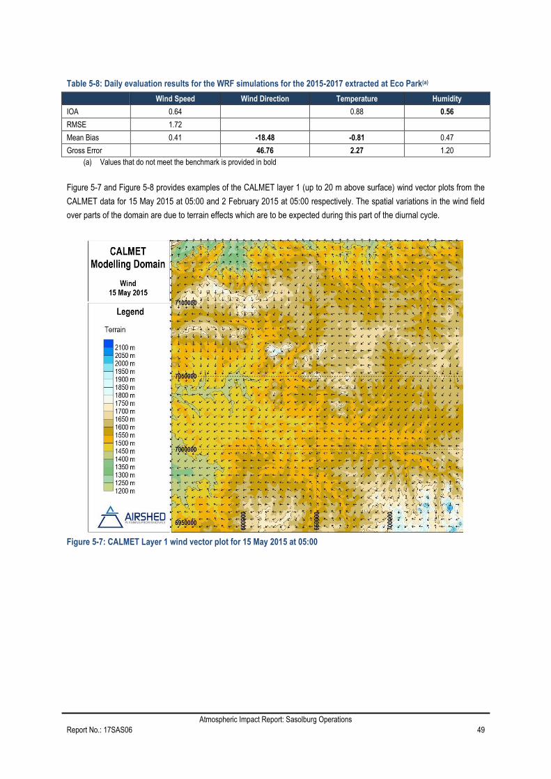
Atmospheric Impact Report: Sasolburg Operations
Report No.: 17SAS06 49
Table 5-8: Daily evaluation results for the WRF simulations for the 2015-2017 extracted at Eco Park(a)
Wind Speed Wind Direction Temperature Humidity
IOA 0.64 0.88 0.56
RMSE 1.72
Mean Bias 0.41 -18.48 -0.81 0.47
Gross Error 46.76 2.27 1.20
(a) Values that do not meet the benchmark is provided in bold
Figure 5-7 and Figure 5-8 provides examples of the CALMET layer 1 (up to 20 m above surface) wind vector plots from the
CALMET data for 15 May 2015 at 05:00 and 2 February 2015 at 05:00 respectively. The spatial variations in the wind field
over parts of the domain are due to terrain effects which are to be expected during this part of the diurnal cycle.
Figure 5-7: CALMET Layer 1 wind vector plot for 15 May 2015 at 05:00

Atmospheric Impact Report: Sasolburg Operations
Report No.: 17SAS06 50
Figure 5-8: CALMET Layer 1 wind vector plot for 2 February 2016 at 05:00
5.1.4.6.2 Land Use and Topographical Data
Readily available terrain and land cover data for use in CALMET was obtained via the Lakes Environmental CALPUFF View
interface. Use was made of Shuttle Radar Topography Mission (SRTM) (30 m, 1 arc-sec) terrain data and Global Land
Cover Characterization (GLCC) land use data for Africa.
Figure 5-9 provides the terrain contours and landuse categories over the entire CALMET domain and the location of the
CALPUFF computational domain.

Atmospheric Impact Report: Sasolburg Operations
Report No.: 17SAS06 51
Figure 5-9: Land use categories, terrain contours, meteorological WRF grid points and surface station locations
displayed on 200 x 200 km CALMET domain (1 km resolution)
5.1.4.6.3 Dispersion Coefficients
The option of dispersion coefficients from internally calculated sigma v, sigma w using micrometeorological variables (u*, w*,
L, etc.) was selected (refer to Appendix E for all CALPUFF control options).
5.1.4.6.4 Grid Resolution and Model Domain
The CALMET modelling domain included an area of 200 km by 200 km with a grid resolution of 1 km. The vertical profile
included 11 vertical levels up to a height of 3 500 m. The CALPUFF model domain selected for the sources at the Sasol
Sasolburg facility included an area of 57 km by 57 km with a grid resolution of 200 m. This area was selected based on the
area of impact around Sasolburg simulated during an assessment undertaken for the Vaal Triangle Airshed Priority Area.
5.1.4.6.5 Building Downwash
The impact of building downwash on ground-level pollutant concentrations was evaluated using “ScreenView" - a Tier 1
screening model which includes the same building downwash scheme as CALPUFF. For the most conservative simulation
of downwind concentrations “ScreenView” was used with a full meteorological set. The SO site was selected for evaluation
due to the relatively short distances between sources and receptors. The screening exercise assessed the individual impact
of three sources selected based on location; stack height; proximity to nearby buildings (excluding complex pipework

Atmospheric Impact Report: Sasolburg Operations
Report No.: 17SAS06 52
structures); and, proximity to receptors. The baseline emission parameters (temperature, release height, exit velocities, etc.)
were used in combination with three theoretical building heights (10, 15, and 20 m). A single emission rate (1 m/s) was used
to simulated the ground-level concentrations at automated distances between 1 m and 5 000 m from the sources, at 100 m
intervals.
The screening assessment indicated that building downwash did not affect downwind concentration as a result of the
boilers, due to height of release (75 m for Steam Station 1). Sources with lower release heights (15 m and 20 m) were found
to increase ground-level concentrations downwind of the source where the scale of increase was dependent on the height of
the near-by building. The distance after which simulate ground-level concentrations matched levels for comparative
simulations where building downwash was not included was a minimum of 1 800 m.
Due to the close proximity between sources, buildings and receptors at the SO facility, building downwash was accounted
for in the dispersion modelling, specifically buildings and sources along the western boundary of the facility, which is within
100 m of a residential area (Table 5-9). The AERMOD Building Profile Input Program (BPIP) module was used to generate a
building downwash input file for CALPUFF where building dimensions were provided by Sasol.
Table 5-9: Parameters of buildings on the SO facility included in the dispersion modelling
Building ID Latitude Longitude Height (m) X length (m) Y length (m) Angle from
North
1 -26.83214 27.84326 10.0 15.0 24.0 332°
2 -26.83169 27.84446 10.1 30.5 50.5 332°
3 -26.83192 27.84290 8.5 30.0 30.0 332°
4 -26.83164 27.84270 37.0 11.2 24.0 332°
5A -26.83199 27.84266 6.0 18.0 19.0 332°
5B -26.83206 27.84254 6.0 12.0 30.0 332°
5C -26.83182 27.84256 9.0 5.0 14.0 332°
6A -26.83197 27.84236 8.0 9.0 14.0 332°
6B -26.83170 27.84233 6.0 7.0 7.0 332°
6C -26.83172 27.84251 6.0 9.0 10.0 332°
7 -26.83188 27.84188 12.0 12.0 3.5 332°
8A -26.83207 27.84156 7.0 6.0 11.0 332°
8B -26.83197 27.84149 4.0 6.0 30.0 332°
9 -26.83156 27.84206 2.0 5.0 12.0 332°
11 -26.83135 27.84253 37.0 40.0 40.0 332°
13 -26.83249 27.84264 5.0 11.0 35.0 332°
16 -26.82605 27.84036 13.0 20.0 32.6 63°
17 -26.82843 27.84057 13.6 32.0 55.0 332°
19 -26.82878 27.84025 13.6 40.0 90.0 332°
20 -26.82874 27.84082 13.0 22.0 25.0 332°
21 -26.82951 27.84067 9.0 16.0 22.0 332°
22 -26.82994 27.84130 10.0 16.8 42.2 22.5°
23 -26.82524 27.83835 10.0 19.9 43.8 332°
24 -26.82574 27.83844 26.6 18.0 20.0 332°
25 -26.82623 27.83830 10.0 17.5 79.2 63°
5.1.5 Atmospheric Dispersion Potential
Meteorological mechanisms govern the dispersion, transformation, and eventual removal of pollutants from the atmosphere.
The analysis of hourly average meteorological data is necessary to facilitate a comprehensive understanding of the
dispersion potential of the site. The horizontal dispersion of pollution is largely a function of the wind field. The wind speed
determines both the distance of downward transport and the rate of dilution of pollutants. A summary of the measured
meteorological data is given in Appendix G.

Atmospheric Impact Report: Sasolburg Operations
Report No.: 17SAS06 53
Sasol currently operates four meteorological stations in the Sasolburg area (viz. Sasol 1 Fence Line, Eco Park, AJ Jacobs
and Leitrim). For this assessment, data from the Sasol operated meteorological stations at Eco Park, AJ Jacobs and Leitrim
was provided for the period 2015 to 2017. Parameters useful in describing the dispersion and dilution potential of the site
(i.e. wind speed, wind direction, temperature and atmospheric stability) are subsequently discussed.
5.1.5.1 Surface Wind Field
Wind roses comprise 16 spokes, which represent the directions from which winds blew during a specific period. The colours
used in the wind roses below, reflect the different categories of wind speeds; the red area, for example, representing winds
>6m/s. The dotted circles provide information regarding the frequency of occurrence of wind speed and direction categories.
The frequency with which calms occurred, i.e. periods during which the wind speed was below 1 m/s are also indicated.
The period wind field and diurnal variability (2015 to 2017) for the three Sasol operated meteorological stations in the
Sasolburg area is provided in Figure 5-10 to Figure 5-12.
The predominant flow field at Eco Park is from the east-southeast (~12% frequency of occurrence). During day-time
conditions winds from the north-western sector increases while winds from the east-southeast are more frequent during
night-time conditions (Figure 5-10).
The predominant wind direction at AJ Jacobs is from the north-northeast (~11% frequency of occurrence) (Figure 5-11).
Very little wind is measured from the south-eastern sector. During day-time conditions winds from the western sector
increase while winds from the north-northeast are more frequent during night-time conditions. A higher frequency of low-
speed winds (1-2 m/s) and calm conditions (less than 1 m/s) was measured at this monitoring station.
The predominant wind direction at Leitrim is from the north-northeast and east (~10% frequency of occurrence). During day-
time conditions winds from the western sector increase while winds from the east, south-southeast and north-northeast are
more frequent during night-time conditions (Figure 5-12).

Atmospheric Impact Report: Sasolburg Operations
Report No.: 17SAS06 54
Figure 5-10: Period, day- and night-time wind rose for Eco Park for the period 2015 - 2017
Figure 5-11: Period, day- and night-time wind rose for AJ Jacobs for the period 2015 - 2017

Atmospheric Impact Report: Sasolburg Operations
Report No.: 17SAS06 55
Figure 5-12: Period, day- and night-time wind rose for Leitrim for the period 2015 - 2017
5.1.5.2 Temperature
Air temperature is important, both for determining the effect of plume buoyancy (the larger the temperature difference
between the emission plume and the ambient air, the higher the plume can rise), and determining the development of the
mixing and inversion layers.
The average monthly temperature trends are presented in Figure 5-13 and Figure 5-14 for Eco Park and Leitrim
respectively. Monthly mean and hourly maximum and minimum temperatures are given in Table 5-9.
Table 5-10: Monthly temperature summary (2015 - 2017)
Hourly Minimum, Hourly Maximum and Monthly Average Temperatures (°C)
(2015 - 2017)
Jan Feb Mar Apr May Jun Jul Aug Sep Oct Nov Dec
Eco Park
Minimum 17.2 16.7 14.7 11.6 6.8 4.0 3.9 5.7 11.4 13.2 14.3 17.1
Maximum 27.1 27.6 26.3 24.2 21.8 19.1 19.3 22.8 25.8 27.3 27.1 28.1
Average 22.1 21.9 20.3 17.5 14.0 11.0 11.2 14.2 18.4 20.3 20.8 22.4
Leitrim
Minimum 17.3 16.7 14.6 11.6 7.1 4.6 4.0 5.6 10.8 13.4 14.1 17.0
Maximum 27.4 28.4 26.6 24.4 22.2 19.2 19.7 23.2 25.8 27.7 27.3 28.4
Average 22.2 22.3 20.3 17.8 14.2 11.4 11.4 14.3 18.1 20.6 20.7 22.5

Atmospheric Impact Report: Sasolburg Operations
Report No.: 17SAS06 56
Average temperatures ranged between 11 °C and 22.5 °C. The highest temperatures occurred in December and the lowest
in July. During the day, temperatures increase to reach maximum at around 15:00 in the afternoon. Ambient air temperature
decreases to reach a minimum at around 07:00 i.e. just before sunrise.
Figure 5-13: Monthly average temperature profile for Eco Park (2015 – 2017)
Figure 5-14: Monthly average temperature profile for Leitrim (2015 – 2017)

Atmospheric Impact Report: Sasolburg Operations
Report No.: 17SAS06 57
5.1.5.3 Atmospheric Stability
The atmospheric boundary layer properties are described by two parameters; the boundary layer depth and the Monin-
Obukhov length.
The Monin-Obukhov length (LMo) provides a measure of the importance of buoyancy generated by the heating of the
ground and mechanical mixing generated by the frictional effect of the earth’s surface. Physically, it can be thought of as
representing the depth of the boundary layer within which mechanical mixing is the dominant form of turbulence generation
(CERC, 2004). The atmospheric boundary layer constitutes the first few hundred metres of the atmosphere. During daytime,
the atmospheric boundary layer is characterised by thermal turbulence due to the heating of the earth’s surface. Night-times
are characterised by weak vertical mixing and the predominance of a stable layer. These conditions are normally associated
with low wind speeds and lower dilution potential.
Diurnal variation in atmospheric stability, as calculated from on-site data (Tiwary and Colls, 2010), and described by the
inverse Monin-Obukhov length and the boundary layer depth is provided in Figure 5-15. The highest concentrations for
ground level, or near-ground level releases from non-wind dependent sources would occur during weak wind speeds and
stable (night-time) atmospheric conditions.
For elevated releases, unstable conditions can result in very high concentrations of poorly diluted emissions close to the
stack. This is called looping (Figure 5-15 (c)) and occurs mostly during daytime hours. Neutral conditions disperse the plume
fairly equally in both the vertical and horizontal planes and the plume shape is referred to as coning (Figure 5-15 (b)). Stable
conditions prevent the plume from mixing vertically, although it can still spread horizontally and is called fanning (Figure 5-14
(a)) (Tiwary & Colls, 2010).
Figure 5-15: Diurnal atmospheric stability (extracted from CALMET at the Eco Park monitoring point)

Atmospheric Impact Report: Sasolburg Operations
Report No.: 17SAS06 58
5.1.5.4 Air Quality Monitoring data
A summary of ambient data measured at Leitrim, AJ Jacobs and Eco Park for the period 2015 – 2017 is provided in Table
5-12, Table 5-13 and Table 5-14 respectively. A summary of ambient air quality data recorded at the DEA stations - Three
Rivers, Sharpeville, and Zamdela - is provided in Table 5-15, Table 5-16, and Table 5-17. Time series of the measured
ambient air quality data is provided in Appendix G.
Table 5-11: Summary of the ambient NH3 measurements at Fence Line for the period 2010-2012 (units: µg/m3)
Period Hourly
Annual Average Max 99th Percentile 90th Percentile 50th Percentile
NH3
2010 231.34 65.19 6.59 0.59 4.74
2011 270.11 82.68 15.98 1.10 6.60
2012 236.77 88.22 23.29 5.18 10.11
Average 246.07 78.69 15.28 2.29 7.15 NOTE: * Ammonia is no longer monitored at the Sasol monitoring stations and therefore data for the most recent available period was used.
Table 5-12: Summary of the ambient measurements at Leitrim for the period 2015-2017 (units: µg/m3)
Period Availability
Hourly Annual Average
No of recorded hourly exceedances Max
99th Percentile
90th Percentile
50th Percentile
NO2
2015 21% 178.4 64.9 39.0 17.3 21.2 1
2016 91% 140.7 87.2 47.8 17.6 22.8 -
2017 90% 117.4 77.9 42.9 15.4 19.2 -
Average 76.7 43.2 16.8 21.1
SO2
2015 85% 1007.4 185.0 82.3 20.0 33.3 4
2016 94% 515.9 205.8 78.5 28.4 39.4 15
2017 90% 425.8 172.6 70.3 24.6 33.5 2
Average 187.8 77.0 24.3 35.4
Period Availability
Daily Annual Average
No of recorded daily exceedances Max
99th Percentile
90th Percentile
50th Percentile
SO2
2015 85% 46.1 40.5 26.9 11.2 33.3 -
2016 94% 45.7 38.2 23.7 14.4 39.4 -
2017 90% 37.1 30.6 22.2 11.8 33.5 -
Average 36.4 24.2 12.4 35.4
PM10
2015 81% 192.1 153.4 106.0 37.7 49.2 57
2016 24% 129.9 121.6 100.9 12.7 38.5 21
2017 52% 193.5 142.4 80.4 29.4 38.0 22
Average 139.1 95.8 26.6 41.9
PM2.5
2015 65% 117.0 75.2 50.0 19.3 24.2 5
2016 26% 59.8 58.5 37.2 2.9 12.6 8
2017 52% 49.7 39.1 22.3 8.1 10.5 2
Average 57.6 36.5 10.1 15.8

Atmospheric Impact Report: Sasolburg Operations
Report No.: 17SAS06 59
Table 5-13: Summary of the ambient measurements at AJ Jacobs for the period 2015-2017 (units: µg/m3)
Period Availability
Hourly Annual Average
No of recorded hourly exceedances Max
99th Percentile
90th Percentile
50th Percentile
NO2
2015 86% 127.4 79.6 46.3 15.3 21.0 -
2016 95% 125.4 73.5 42.9 16.1 20.3 -
2017 92% 164.7 81.4 52.1 25.1 26.6 -
Average 78.1 47.1 18.8 22.7
SO2
2015 98% 603.6 284.1 111.1 46.3 56.3 34
2016 96% 676.0 307.7 121.1 41.0 57.2 54
2017 88% 718.5 320.6 173.4 78.0 89.7 56
Average 304.1 135.2 55.1 67.7
Period Availability
Daily Annual Average
No of recorded daily exceedances Max
99th Percentile
90th Percentile
50th Percentile
SO2
2015 98% 224.6 152.9 104.5 53.5 56.3 14
2016 96% 188.0 162.1 103.0 49.1 57.2 23
2017 88% 220.6 194.5 160.0 80.5 89.7 91
Average 169.9 122.5 61.0 67.7
PM10
2015 96% 124.6 119.9 81.1 39.5 46.4 48
2016 99% 154.9 105.1 76.1 37.7 43.1 39
2017 98% 107.3 94.6 74.0 33.4 38.9 32
Average 106.5 77.1 36.9 42.8
PM2.5
2015 93% 51.0 48.2 30.9 16.1 18.3 -
2016 82% 73.7 54.2 33.4 15.2 17.9 14
2017 93% 75.8 69.9 49.7 19.9 24.8 66
Average 57.5 38.0 17.1 20.4
Table 5-14: Summary of the ambient measurements at Eco Park for the period 2015-2017 (units: µg/m3)
Period Availability
Hourly Annual Average
No of recorded hourly exceedances Max
99th Percentile
90th Percentile
50th Percentile
NO2
2015 84% 782.9 85.1 52.9 15.9 22.3 2
2016 98% 373.1 85.9 51.1 15.0 21.5 6
2017 98% 439.8 84.2 49.2 14.4 20.5 3
Average 85.1 51.1 15.1 21.5
SO2
2015 96% 881.5 239.4 89.9 42.8 51.5 31
2016 98% 842.4 261.8 82.6 28.3 41.9 41
2017 98% 891.5 230.4 65.5 21.2 33.4 35
Average 243.8 79.3 30.8 42.2
Period Availability
Daily Annual Average
No of recorded daily exceedances Max
99th Percentile
90th Percentile
50th Percentile
SO2
2015 96% 131.0 117.6 86.1 48.8 51.5 1
2016 98% 144.3 128.1 81.5 36.3 41.9 5
2017 98% 145.6 100.9 60.4 30.0 33.4 2
Average 115.5 76.0 38.3 42.2
PM10
2015 93% 150.4 126.1 83.0 27.5 37.2 45
2016 98% 131.1 117.9 69.5 27.2 33.1 29

Atmospheric Impact Report: Sasolburg Operations
Report No.: 17SAS06 60
Period Availability
Hourly Annual Average
No of recorded hourly exceedances Max
99th Percentile
90th Percentile
50th Percentile
2017 96% 145.5 98.3 68.5 23.3 31.4 29
Average 112.6 71.9 26.5 34.0
PM2.5
2015 95% 61.7 52.6 35.2 14.7 18.2 -
2016 98% 312.9 308.8 32.9 13.3 20.6 23
2017 97% 331.9 69.8 46.1 16.3 22.0 50
Average 143.7 38.1 14.7 20.3
O3
2015 98% 124.1 109.7 85.5 58.7 58.3
2016 99% 1567.4 728.0 91.3 58.0 79.5
2017 99% 112.3 108.0 85.3 60.0 61.2
Average 315.2 87.4 58.9 67.0
Table 5-15: Summary of the ambient measurements at Three Rivers for the period 2015-2017 (units: µg/m3)
Period Availability
Hourly Annual Average
No of recorded hourly exceedances Max
99th Percentile
90th Percentile
50th Percentile
NO2
2015 80% 178.6 104.6 64.5 24.8 31.5 -
2016 91% 148.4 92.1 53.0 21.8 26.4 -
2017 91% 178.2 95.1 54.3 20.8 26.3 -
Average 97.3 57.3 22.5 28.1
SO2
2015 53% 592.0 110.1 30.3 8.0 14.5 5
2016 91% 474.8 163.1 30.4 7.6 15.5 7
2017 91% 539.3 141.5 36.2 10.1 17.9 9
Average 138.3 32.3 8.6 16.0
Benzene
2015 37% 17.3 6.7 3.7 0.4 1.2
2016 83% 11.6 3.0 1.2 0.1 0.4
2017 79% 13.2 2.8 0.8 0.1 0.3
Average 4.2 1.9 0.2 0.7
CO
2015 83% 5710 1808 715 260 352 -
2016 91% 5250 1482 896 496 587 -
2017 44% 3769 1632 979 549 658 -
Average 1641 863 435 532
Period Availability
Daily Annual Average
No of recorded daily exceedances Max
99th Percentile
90th Percentile
50th Percentile
SO2
2015 53% 105.2 55.4 26.9 10.8 14.5 -
2016 91% 117.7 67.3 32.7 11.0 15.5 -
2017 91% 114.2 72.4 33.0 14.3 17.9 -
Average 65.0 30.9 12.0 16.0
PM10
2015 82% 144.2 119.3 84.3 46.2 51.4 54
2016 90% 174.2 130.1 101.8 53.7 61.1 87
2017 90% 248.4 177.6 63.5 32.0 38.6 24
Average 142.3 83.3 43.9 50.4
PM2.5
2015 87% 76.6 69.7 45.7 25.6 27.7 5
2016 82% 96.5 61.8 45.8 26.0 28.7 58
2017 78% 83.0 60.1 34.7 21.0 22.1 18
Average 63.8 42.0 24.2 26.2

Atmospheric Impact Report: Sasolburg Operations
Report No.: 17SAS06 61
O3
2015 80% 127.8 105.2 85.0 55.9 55.6
2016 89% 122.8 104.0 83.9 55.5 56.4
2017 45% 107.5 76.3 64.4 43.7 44.0
Average 95.2 77.8 51.7 52.0
Table 5-16: Summary of the ambient measurements at Sharpeville for the period 2015-2017 (units: µg/m3)
Period Availability
Hourly Annual Average
No of recorded hourly exceedances Max
99th Percentile
90th Percentile
50th Percentile
NO2
2015 86% 344.0 156.7 96.3 31.3 43.9 15
2016 86% 176.8 104.7 62.7 22.6 29.7 -
2017 82% 195.5 105.2 64.1 21.8 29.6 -
Average 122.2 74.4 25.2 34.4
SO2
2015 87% 950.4 135.8 38.2 10.9 19.1 16
2016 80% 512.3 127.1 34.0 7.0 15.2 3
2017 69% 462.8 180.7 49.0 8.8 20.8 6
Average 147.9 40.4 8.9 18.4
Benzene
2015 32% 25.9 12.2 3.1 0.5 1.3
2016 0%
2017 35% 56.1 16.8 5.4 0.8 2.1
Average 14.5 4.3 0.6 1.7
CO
2015 87% 6420 3492 1516 512 712 -
2016 88% 7684 3724 1903 739 968 -
2017 44% 5736 3317 1647 701 893 -
Average 3511 1688 651 858
Period Availability
Daily Annual Average
No of recorded daily exceedances Max
99th Percentile
90th Percentile
50th Percentile
SO2
2015 87% 135.0 94.0 36.5 13.4 19.1 2
2016 80% 97.6 74.5 33.5 9.7 15.2 -
2017 69% 147.1 106.6 46.5 12.4 20.8 1
Average 91.7 38.8 11.8 18.4
PM10
2015 89% 178.0 153.6 110.3 53.8 62.8 83
2016 86% 251.0 234.8 166.9 84.6 95.9 185
2017 56% 188.5 130.5 84.1 41.8 46.7 36
Average 173.0 120.4 60.1 68.5
PM2.5
2015 88% 138.4 97.9 60.6 31.8 36.5 27
2016 53% 81.7 77.2 47.1 29.7 31.6 43
2017 90% 322.4 151.1 68.3 34.6 39.4 131
Average 108.7 58.7 32.0 35.8
O3
2015 88% 127.8 107.3 83.5 52.1 51.3
2016 91% 107.9 103.8 72.9 45.9 48.3
2017 50% 99.3 96.5 81.5 49.6 52.5
Average 102.5 79.3 49.2 50.7

Atmospheric Impact Report: Sasolburg Operations
Report No.: 17SAS06 62
Table 5-17: Summary of the ambient measurements at Zamdela for the period 2015-2017 (units: µg/m3)
Period Availability
Hourly Annual Average
No of recorded hourly exceedances Max
99th Percentile
90th Percentile
50th Percentile
NO2
2015 87% 168.1 100.4 62.4 24.6 30.1 -
2016 88% 199.8 123.7 73.7 24.3 32.7 -
2017 50% 141.7 91.3 55.8 21.3 26.4 -
Average 105.2 64.0 23.4 29.7
SO2
2015 87% 414.5 172.7 52.4 9.2 21.4 5
2016 87% 647.7 187.1 52.9 9.9 22.2 5
2017 75% 356.1 165.5 44.3 8.2 18.7 2
Average 175.1 49.8 9.1 20.7
Benzene
2015 63% 16.3 11.6 4.2 1.0 1.8
2016 67% 2752.4 638.8 220.8 0.9 59.5
2017 49% 31.5 25.9 7.7 1.3 3.1
Average 225.4 77.6 1.1 21.4
CO
2015 73% 7187 3889 1267 491 652 -
2016 84% 12691 4860 1491 645 858 -
2017 38% 7690 3965 1432 703 845 -
Average 4238 1397 613 785
Period Availability
Daily Annual Average
No of recorded daily exceedances Max
99th Percentile
90th Percentile
50th Percentile
SO2
2015 87% 105.1 68.2 43.6 17.9 21.4 -
2016 87% 180.7 81.1 44.9 17.2 22.2 2
2017 75% 171.8 68.9 41.9 13.0 18.7 1
Average 75.3 44.5 17.8 22.3
PM10
2015 57% 221.9 125.2 88.7 40.3 46.0 35
2016 92% 175.3 165.2 106.5 57.2 64.7 106
2017 76% 245.2 133.1 74.7 46.5 49.4 26
Average 141.1 90.0 48.0 53.3
PM2.5
2015 80% 93.6 73.2 54.2 26.0 30.0 11
2016 82% 138.4 95.8 58.7 30.9 35.0 92
2017 83% 105.9 89.8 45.9 26.9 29.7 64
Average 86.3 52.9 27.9 31.6
O3
2015 94% 95.7 88.0 71.3 49.1 50.4
2016 95% 91.8 83.3 67.4 43.9 45.9
2017 41% 77.4 71.8 53.0 35.0 35.7
Average 81.0 63.9 42.7 44.0
The following graphs summarise the observed concentrations of SO2, NO2, and PM10 at the six monitoring sites (Leitrim, AJ
Jacobs, Eco Park, Three Rivers, Sharpeville, and Zamdela) monitoring stations for the years 2015, 2016 and 2017. The
NAAQS have been included in the graphs for:
• SO2 hourly (88 hourly exceedances of 350 µg/m³) and daily average (4 daily exceedances of 125 µg/m³)
• NO2 hourly average (88 hourly exceedances of 200 µg/m³); and,
• PM10 daily average (4 daily exceedances of 75 µg/m³; 2015 standards).

Atmospheric Impact Report: Sasolburg Operations
Report No.: 17SAS06 63
The hourly 99th percentiles for SO2 were below the limit value of 350 µg/m³ at all stations for all three years (Figure 5-16 to
Figure 5-21). The daily 99th percentiles for SO2 were exceeded at AJ Jacobs for 2015, 2016 and 2017 (Figure 5-23) and at
Eco Park in 2016 (Figure 5-24) but were below the limit value (125 µg/m³) at Leitrim, Three Rivers, Sharpeville and Zamdela
stations for all three years (Figure 5-22 and Figure 5-25 to Figure 5-27).
Figure 5-16: Observed hourly average SO2 concentrations at Leitrim
Figure 5-17: Observed hourly average SO2 concentrations at AJ Jacobs

Atmospheric Impact Report: Sasolburg Operations
Report No.: 17SAS06 64
Figure 5-18: Observed hourly average SO2 concentrations at Eco Park
Figure 5-19: Observed hourly average SO2 concentrations at Three Rivers

Atmospheric Impact Report: Sasolburg Operations
Report No.: 17SAS06 65
Figure 5-20: Observed hourly average SO2 concentrations at Sharpeville
Figure 5-21: Observed hourly average SO2 concentrations at Zamdela

Atmospheric Impact Report: Sasolburg Operations
Report No.: 17SAS06 66
Figure 5-22: Observed daily average SO2 concentrations at Leitrim
Figure 5-23: Observed daily average SO2 concentrations at AJ Jacobs

Atmospheric Impact Report: Sasolburg Operations
Report No.: 17SAS06 67
Figure 5-24: Observed daily average SO2 concentrations at Eco Park
Figure 5-25: Observed daily average SO2 concentrations at Three Rivers

Atmospheric Impact Report: Sasolburg Operations
Report No.: 17SAS06 68
Figure 5-26: Observed daily average SO2 concentrations at Sharpeville
Figure 5-27: Observed daily average SO2 concentrations at Zamdela
The hourly 99th percentiles for NO2 were below the limit value (200 µg/m³) at all stations and for all three years (Figure 5-28
to Figure 5-33).
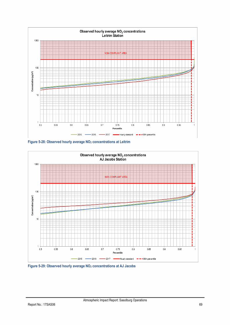
Atmospheric Impact Report: Sasolburg Operations
Report No.: 17SAS06 69
Figure 5-28: Observed hourly average NO2 concentrations at Leitrim
Figure 5-29: Observed hourly average NO2 concentrations at AJ Jacobs

Atmospheric Impact Report: Sasolburg Operations
Report No.: 17SAS06 70
Figure 5-30: Observed hourly average NO2 concentrations at Eco Park
Figure 5-31: Observed hourly average NO2 concentrations at Three Rivers

Atmospheric Impact Report: Sasolburg Operations
Report No.: 17SAS06 71
Figure 5-32: Observed hourly average NO2 concentrations at Sharpeville
Figure 5-33: Observed hourly average NO2 concentrations at Zamdela
The daily 99th percentiles for PM10 exceed the limit value (75 µg/m³; 2015 standard) at all stations and for all three years
(Figure 5-34 to Figure 5-39). Non-compliance varied between 3% and 50% of the three years assessed.

Atmospheric Impact Report: Sasolburg Operations
Report No.: 17SAS06 72
Figure 5-34: Observed daily average PM10 concentrations at Leitrim
Figure 5-35: Observed daily average PM10 concentrations at AJ Jacobs

Atmospheric Impact Report: Sasolburg Operations
Report No.: 17SAS06 73
Figure 5-36: Observed daily average PM10 concentrations at Eco Park
Figure 5-37: Observed daily average PM10 concentrations at Three Rivers

Atmospheric Impact Report: Sasolburg Operations
Report No.: 17SAS06 74
Figure 5-38: Observed daily average PM10 concentrations at Sharpeville
Figure 5-39: Observed daily average PM10 concentrations at Zamdela
Time variation plots (mean with 95% confidence interval) of ambient SO2, NO2, and particulate matter (PM10 and PM2.5)
concentrations measured the six monitoring stations show the variation of these pollutants over a daily, weekly and annual
cycles (Figure 5-40 to Figure 5-51). The daily SO2 show a typically industrial signature with increased SO2 concentrations as

Atmospheric Impact Report: Sasolburg Operations
Report No.: 17SAS06 75
just before midday due to the break-up of an elevated inversion layer, in addition to the development of daytime convective
conditions causing the plume to be brought down to ground level relatively close to the point of release from tall stacks.
Increased NO2 concentrations during peak traffic times (07:00 to 08:00 and 16:00 to 18:00) illustrate the contribution of
vehicle emissions to the ambient NO2 concentrations. The winter (June, July and August) elevation of SO2 and NO2 shows
the contribution of residential fuel burning to the ambient SO2 and NO2 concentrations.
Monthly variation of particulate matter shows elevated concentrations during winter months due to the larger contribution
from domestic fuel burning, dust from uncovered soil and the lack of the settling influence of rainfall (Figure 5-46 and Figure
5-51).

Atmospheric Impact Report: Sasolburg Operations
Report No.: 17SAS06 76
Figure 5-40: Time variation plot of observed SO2 and NO2 concentrations at Leitrim (shaded area indicates 95th percentile confidence interval)

Atmospheric Impact Report: Sasolburg Operations
Report No.: 17SAS06 77
Figure 5-41: Time variation plot of observed SO2 and NO2 concentrations at AJ Jacobs (shaded area indicates 95th percentile confidence interval)

Atmospheric Impact Report: Sasolburg Operations
Report No.: 17SAS06 78
Figure 5-42: Time variation plot of observed SO2 and NO2 concentrations at Eco Park (shaded area indicates 95th percentile confidence interval)

Atmospheric Impact Report: Sasolburg Operations
Report No.: 17SAS06 79
Figure 5-43: Time variation plot of observed SO2 and NO2 concentrations at Three Rivers (shaded area indicates 95th percentile confidence interval)

Atmospheric Impact Report: Sasolburg Operations
Report No.: 17SAS06 80
Figure 5-44: Time variation plot of observed SO2 and NO2 concentrations at Sharpeville (shaded area indicates 95th percentile confidence interval)

Atmospheric Impact Report: Sasolburg Operations
Report No.: 17SAS06 81
Figure 5-45: Time variation plot of observed SO2 and NO2 concentrations at Zamdela (shaded area indicates 95th percentile confidence interval)
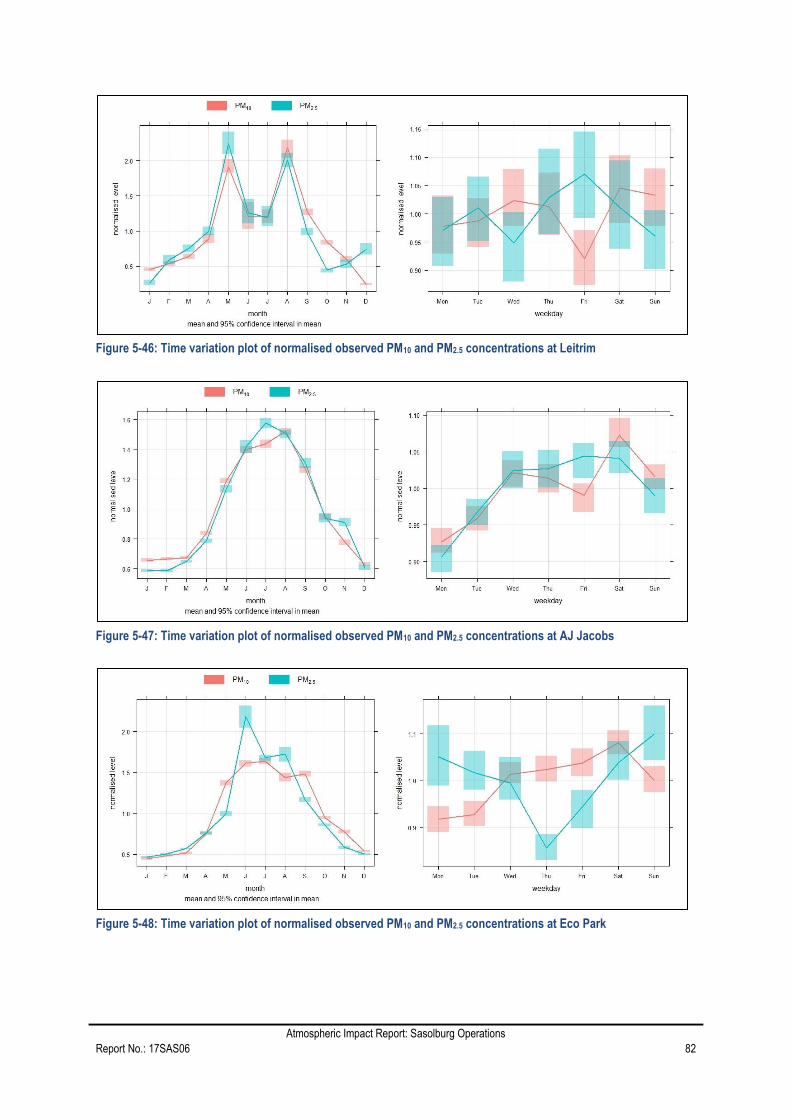
Atmospheric Impact Report: Sasolburg Operations
Report No.: 17SAS06 82
Figure 5-46: Time variation plot of normalised observed PM10 and PM2.5 concentrations at Leitrim
Figure 5-47: Time variation plot of normalised observed PM10 and PM2.5 concentrations at AJ Jacobs
Figure 5-48: Time variation plot of normalised observed PM10 and PM2.5 concentrations at Eco Park

Atmospheric Impact Report: Sasolburg Operations
Report No.: 17SAS06 83
Figure 5-49: Time variation plot of normalised observed PM10 and PM2.5 concentrations at Three Rivers
Figure 5-50: Time variation plot of normalised observed PM10 and PM2.5 concentrations at Sharpeville
Figure 5-51: Time variation plot of normalised observed PM10 and PM2.5 concentrations at Zamdela

Atmospheric Impact Report: Sasolburg Operations
Report No.: 17SAS06 84
5.1.6 Model Performance
5.1.6.1 Understanding of Observed Concentrations
An analysis of the observed SO2, NO2 and PM10 concentrations at six monitoring stations was completed, in which the
concentration values were categorised into wind speed and direction bins for different concentrations. This information is
most easily visualised as polar plots, where the centre of the polar plot refers to the location of the monitoring station, as
shown in Figure 5-52 for Leitrim and Figure 5-54 for Eco Park for SO2 observations (other stations Figure 5-55 to Figure
5-57). The corresponding NO2 analyses are summarised in Figure 5-58 to Figure 5-63. Polar plots for PM analyses are
presented in Figure 5-64 and Figure 5-69.
These polar plots (Carslaw and Ropkins, 2012; Carslaw, 2013) provide an indication of the directional contribution as well as
the dependence of concentrations on wind speed. Whereas the directional display is fairly obvious, i.e. when higher
concentrations are shown to occur in a certain sector, e.g. east and south for SO2 at Eco Park (Figure 5-54), it is understood
that most of the high concentrations occur when winds blow from that sector (i.e. east or south). When the high
concentration pattern is more symmetrical around the centre of the plot, it is an indication that the contributions are near-
equally distributed, as is displayed for SO2 in Figure 5-55.
Furthermore, since the observed concentrations have also been categorised according to wind speed categories, it provides
an indication of the plume height. As explained in Section 5.1.4.1 (plume buoyancy), stronger winds reduce the amount of
plume rise, and may effectively increase ground level concentrations. However, since an increased wind speed also
enhances plume dispersion, a concentration maximum would be reached for a wind speed where the plume rise and dilution
effects cancel each other. These conditions would be different for day- and night-time atmospheric stabilities. It is expected
that high ground level concentrations from elevated stacks would be more prevalent during stronger wind speeds during
stable conditions than daytime, convective conditions, when the plume buoyancy is often not as effective in lifting the plume
centreline. Low-level emissions behave differently, and higher concentrations would normally be observed during weak-wind
conditions.
The SO2 concentrations observed at Leitrim (Figure 5-52) show elevated concentrations occurring with north-easterly winds
above 5 m/s. Sasol operations are located towards the north-west and the increased concentrations due to emissions from
this direction are also evident at wind speeds above 2 m/s. Other SO2 contributions originate to the north-west of the Leitrim
station. The dominant contribution of median SO2 concentrations above 100 μg/m³ originate to the north-east of the AJ
Jacobs at wind speeds between 2 m/s and 8 m/s (Figure 5-53). The SO2 concentrations observed at Eco Park (Figure 5-54)
indicate that most of the high concentrations occur with easterly winds between 6 m/s and 10 m/s. Albeit not as high as the
concentrations from the easterly sector, the observations also show elevated concentrations from an southerly direction.
The Three Rivers station recorded relatively low median hourly SO2 concentrations from all directions (Figure 5-55). Median
SO2 concentrations above 50 μg/m³ originate from the east and north-west at wind speeds above 2 m/s at the Sharpeville
station (Figure 5-56). The Zamdela station recorded elevated SO2 concentrations (above 100 μg/m³) at wind speeds above
6 m/s from the north-east (Figure 5-57). Other SO2 contributions originate to the north-west and north of the Zamdela
station.
The NO2 concentrations observed at Leitrim (Figure 5-58) indicate that most of the elevated concentrations occur from the
north-westerly winds of between 2 m/s and 6 m/s, northerly winds at winds less than 2 m/s or above 10 m/s. Since vehicular
exhaust emissions are significant NO2 contributors, the observations from the northern sector most likely indicates this
source. Median NO2 concentrations originate to the north-east of the AJ Jacobs at all wind speeds (Figure 5-59). The NO2
concentrations observed at Eco Park (Figure 5-60) showed higher concentrations occurring during relatively weak winds of

Atmospheric Impact Report: Sasolburg Operations
Report No.: 17SAS06 85
about 2 m/s and at higher wind speeds around 10 m/s, primarily from the south-south-west of the station. Median NO2
concentrations observed at the Three Rivers station showed a local source at low wind speeds contributing NO2
concentrations of approximately 50 μg/m³ (Figure 5-61). Higher NO2 concentrations were recorded during high wind speeds
(above 8 m/s) from the east of the Three Rivers station. A similar pattern of a local NO2 source at low wind speeds is evident
at the Sharpeville station (Figure 5-62), while NO2 concentrations above 50 μg/m³ originate to the west-north-west of the
Sharpeville station at wind speeds 8 m/s. Median NO2 concentrations measured at the Zamdela station show contributions
of NO2 above 50 μg/m³ from the north-west and north east at all wind speeds (Figure 5-63).
Elevated particulate concentrations at Leitrim show contributions from the north and north-west at higher (between 8 and
10 m/s) wind speeds (Figure 5-64). At low wind speeds (2 m/s or less) the almost symmetrical plot shows a local
contribution, most likely a result of community activities. Elevated particulate matter concentrations at AJ Jacobs are shown
to originate from the northerly sector at wind speeds above 3 m/s (Figure 5-65). Other sources of particulate matter
contribute to concentrations of approximately 50 µg/m³ from localised sources at wind speeds below 1 m/s. Particulate
concentrations observed at the Eco Park station are lower than at the other stations, where the sources of elevated
concentrations (greater than 40 μg/m³) are located to the north-west of the station (Figure 5-66). Other particulate sources
are also located to the north-east and south-west of the Eco Park station contributing at lower wind speeds (5 to 10 m/s). A
local source also contributes at low wind speeds. The Three Rivers station recorded elevated particulate concentrations
from almost all directions at wind speeds greater than 3 m/s (Figure 5-67). A local source contributes at wind speeds lower
than 2 m/s. Similarly, the Sharpeville station recorded elevated particulate concentrations from nearly all wind directions at
speeds greater than 4 m/s, with the southerly direction showing the lower particulate concentrations (Figure 5-68). A local
source (possibly community activities) is a large contributor at low wind speeds (less than 2 m/s). Particulate concentrations
recorded at the Zamdela show high concentrations from the north-west and north-east, at high wind speeds (above 4 m/s),
and a local source at low wind speeds (Figure 5-69). Sources in the south-westerly sector contribute the lowest
concentrations, especially at higher wind speeds.

Atmospheric Impact Report: Sasolburg Operations
Report No.: 17SAS06 86
Figure 5-52: Polar plot of hourly median SO2 concentration observations at Leitrim for 2015 to 2017
Figure 5-53: Polar plot of hourly median SO2 concentration observations at AJ Jacobs for 2015 to 2017

Atmospheric Impact Report: Sasolburg Operations
Report No.: 17SAS06 87
Figure 5-54: Polar plot of hourly median SO2 concentration observations at Eco Park for 2015 to 2017
Figure 5-55: Polar plot of hourly median SO2 concentration observations at Three Rivers for 2015 to 2017

Atmospheric Impact Report: Sasolburg Operations
Report No.: 17SAS06 88
Figure 5-56: Polar plot of hourly median SO2 concentration observations at Sharpeville for 2015 to 2017
Figure 5-57: Polar plot of hourly median SO2 concentration observations at Zamdela for 2015 to 2017

Atmospheric Impact Report: Sasolburg Operations
Report No.: 17SAS06 89
Figure 5-58: Polar plot of hourly median NO2 concentration observations at Leitrim for 2015 to 2017
Figure 5-59: Polar plot of hourly median NO2 concentration observations at AJ Jacobs for 2015 to 2017
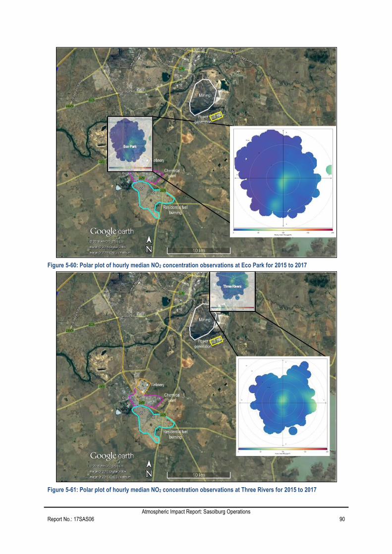
Atmospheric Impact Report: Sasolburg Operations
Report No.: 17SAS06 90
Figure 5-60: Polar plot of hourly median NO2 concentration observations at Eco Park for 2015 to 2017
Figure 5-61: Polar plot of hourly median NO2 concentration observations at Three Rivers for 2015 to 2017

Atmospheric Impact Report: Sasolburg Operations
Report No.: 17SAS06 91
Figure 5-62: Polar plot of hourly median NO2 concentration observations at Sharpeville for 2015 to 2017
Figure 5-63: Polar plot of hourly median NO2 concentration observations at Zamdela for 2015 to 2017

Atmospheric Impact Report: Sasolburg Operations
Report No.: 17SAS06 92
Figure 5-64: Polar plot of hourly median PM10 concentration observations at Leitrim for 2015 to 2017
Figure 5-65: Polar plot of hourly median PM10 concentration observations at AJ Jacobs for 2015 to 2017
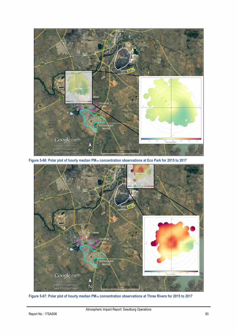
Atmospheric Impact Report: Sasolburg Operations
Report No.: 17SAS06 93
Figure 5-66: Polar plot of hourly median PM10 concentration observations at Eco Park for 2015 to 2017
Figure 5-67: Polar plot of hourly median PM10 concentration observations at Three Rivers for 2015 to 2017
Atmospheric Impact Report: Sasolburg Operations
Report No.: 17SAS06 94
Figure 5-68: Polar plot of hourly median PM10 concentration observations at Sharpeville for 2015 to 2017
Figure 5-69: Polar plot of hourly median PM10 concentration observations at Zamdela for 2015 to 2017

Atmospheric Impact Report: Sasolburg Operations
Report No.: 17SAS06 95
5.1.6.2 Model Validation
Ambient concentrations of NO2, SO2, and PM10 measured by Sasol and the DEA in Sasolburg help provide an
understanding of existing ambient air concentrations as well as providing a means of verifying the dispersion modelling.
Since the aim of the investigation is to illustrate the change in ground level concentrations from the current levels (i.e.
baseline emission scenario) to those levels resulting from the introduction of the required emission limits (i.e. new plant
emission standards), the intention was not to comprehensively include all air emissions within Sasolburg. Unaccounted
emissions include those from unintended leaks within the plant (fugitive emissions) and small vents, as well as air emissions
from other industries, emissions from activities occurring within the communities, and biomass burning (especially during
winter season), as well as long-range transport into the modelling domain. However, information about community activities,
such as the amount of traffic within the community and the amount of fuel used for heating is often difficult to estimate.
These emissions, when combined, may potentially add up to be a significant portion of the observed concentrations in the
modelling domain. In terms of the current investigation, the portion of air quality due to air emission sources that is not
included in the model’s emissions inventory constitutes the background concentration.
Discrepancies between predicted and observed concentrations may also be as a result of process emission variations and
may include upset emissions and shutdowns. These conditions could result in significant under-estimating or over-
estimating the air concentrations. In order to accommodate these upset emission conditions, a time varying emissions
database would be required as input into the model.
A summary of the predicted concentrations (SO and Natref) and their comparison with observations are given in Appendix
H. In order to establish model performance under average emission conditions, it is not uncommon to use a certain
percentile of predicted and observed concentrations for comparison. Although these may range from a 90th to 99.9th
percentile, it was decided to use the DEA NAAQS for guidance. For criteria pollutants SO2, NO2 and PM10, the NAAQS
requires compliance with the 99th percentile. As hourly averages, this allows exceedances of the limit value of 88 hours (SO2
and NO2) or 4 days (SO2 and PM10) per year. Estimated short-term (hourly or daily) background concentrations (not
associated with the emissions included in the simulations) used the observed concentration value when simulated
concentrations from SO indicate very small contributions (0.1 µg/m³).
Table 5-18Table 5-18 summarises the comparisons between simulated (SO and Natref) and observed SO2 concentrations
at the monitoring stations in the study area. As shown in the table of the observed peak concentrations, 72% and 37% could
not be accounted for at Leitrim and AJ Jacobs (the two closest monitoring stations to SO). The difference between simulated
and observation increases significantly when considering long-term comparisons (i.e. 50th percentile and annual average) at
these 2 stations, clearly illustrating the contribution of emission sources not included in the dispersion model’s emissions
inventory.

Atmospheric Impact Report: Sasolburg Operations
Report No.: 17SAS06 96
Table 5-18: Comparison of predicted and observed SO2 concentrations at monitoring station in Sasolburg
Description SO2 concentration (µg/m³)
Unaccounted Fraction* Simulated Observed Unaccounted
Leitrim
Peak 182 650 467 0.7
99th Percentile 67 187 120 0.6
90th Percentile 22 77 55 0.7
50th Percentile 0.01 24 24 1.0
Annual Average 4 35 31 0.9
AJ Jacobs
Peak 422 666 244 0.4
99th Percentile 170 304 134 0.4
90th Percentile 8 135 127 0.9
50th Percentile 0.00 55 55 1.0
Annual Average 6 68 61 0.9
Eco Park
Peak 214 872 658 0.8
99th Percentile 44 244 200 0.8
90th Percentile 1 79 78 1.0
50th Percentile 0.00 31 31 1.0
Annual Average 1 42 41 1.0
Three Rivers
Peak 31 535 504 0.9
99th Percentile 11 138 127 0.9
90th Percentile 0.5 32 32 1.0
50th Percentile 0.00 9 9 1.0
Annual Average 0.3 16 16 1.0
Sharpeville
Peak 47 642 595 0.9
99th Percentile 14 148 134 0.9
90th Percentile 0.6 40 40 1.0
50th Percentile 0.00 9 9 1.0
Annual Average 0.4 18 18 1.0
Zamdela
Peak 301 473 172 0.4
99th Percentile 98 175 76 0.4
90th Percentile 31 50 19 0.4
50th Percentile 0.05 9 9 1.0
Annual Average 7 21 14 0.7
* unaccounted fraction as a percentage of observed concentration
In Figure 5-70, the fractional bias is plotted with the means on the X-axis and the standard deviations on the Y-axis. The box
on the plot encloses the area of the graph where the model predictions are within a fractional bias between -2 and +2;
indicating an acceptable correlation. The U.S. EPA states that predictions within a factor of two are a reasonable
Atmospheric Impact Report: Sasolburg Operations
Report No.: 17SAS06 97
performance target for a model before it is used for refined regulatory analysis (U.S. EPA 1992). Data points appearing on
the left half of the plot indicate an over-prediction and those on the right half of the plot represent under-predictions.
The fractional bias of the means was less than 0.67, clearly showing good model performance at AJ Jacobs and Zamdela.
At Three Rivers, Sharpeville, Leitrim and Eco Park the fractional bias of the means was less than 2, indicating an acceptable
correlation.
Figure 5-70: Fractional bias of means and standard deviation for SO2
The same calculations and comparisons were repeated for NO2 simulations and observations. The CALPUFF simulations
were specifically for NOx and the formation of HNO3 and other nitrates using the MESOPUFF II chemical transformation
mechanism, as discussed in Section 5.1.4.3.
Table 5-19 summarises of comparisons between simulated and observed NO2 concentrations at the monitoring stations in
the study area. For Zamdela, AJ Jacobs and Leitrim higher concentrations were simulated than the observed peak and 99th
percentile concentrations. This may be due to the rather simplistic methodology of applying a constant conversion rate from
NOx to NO2 (Section 5.1.4.3). As shown in Appendix F, the conversion ratio at high concentration levels (i.e. closer to the
point of emission) generally varies between 14% and 27% for NOx concentrations above 188 µg/m³. In this investigation, a
NO2 conservative ratio of not less than 40% was adopted for high concentrations of NOx. Concentrations similar to the
observed peak would be simulated if the lower conversions of 27% were used instead.

Atmospheric Impact Report: Sasolburg Operations
Report No.: 17SAS06 98
As for SO2, the difference between simulated and observation NO2 concentrations increases significantly when considering
long-term comparisons (i.e. 50th percentile and annual average), clearly illustrating the contribution of emission sources not
included in the dispersion model’s emissions inventory.
Table 5-19: Comparison of predicted and observed NO2 concentrations at monitoring stations in Sasolburg
Description NO2 concentration (µg/m³)
Unaccounted Fraction* Simulated Observed Unaccounted
Leitrim
Peak 133 145 12 0.08
99th Percentile 58 77 19 0.25
90th Percentile 23 43 21 0.48
50th Percentile 0.01 17 17 1.00
Annual Average 7 21 14 0.66
AJ Jacobs
Peak 255 139 0 0.00
99th Percentile 111 78 0 0.00
90th Percentile 16 47 31 0.65
50th Percentile 0.00 19 19 1.00
Annual Average 8 23 15 0.65
Eco Park
Peak 136 532 396 0.74
99th Percentile 44 85 41 0.49
90th Percentile 2 51 49 0.97
50th Percentile 0.00 15 15 1.00
Annual Average 2 21 20 0.92
Three Rivers
Peak 51 168 117 0.70
99th Percentile 13 97 84 0.87
90th Percentile 0.6 57 57 0.99
50th Percentile 0.00 23 23 1.00
Annual Average 0.5 28 28 0.98
Sharpeville
Peak 79 208 129 0.62
99th Percentile 18 106 87 0.83
90th Percentile 0.8 64 64 0.99
50th Percentile 0.00 22 22 1.00
Annual Average 0.8 30 29 0.97
Zamdela
Peak 203 170 0 0.00
99th Percentile 62 105 43 0.41
90th Percentile 38 64 26 0.41
50th Percentile 0.08 23 23 1.00
Annual Average 10 30 19 0.65
* unaccounted fraction as a percentage of observed concentration
Atmospheric Impact Report: Sasolburg Operations
Report No.: 17SAS06 99
In contrast to Zamdela, AJ Jacobs and Leitrim, where the peak concentration was definitely shown to be from SO and
Natref, only about 26%, 30% and 38% of the observed concentration was simulated at Eco Park, Three Rivers and
Sharpeville respectively. Although this may still have resulted from SO and Natref, there is also a strong likelihood that more
localised sources may have added to the observed peak. Other sources of NO2 concentrations are also observed at these
sites in the polar plots (Figure 5-60 for Eco Park, Figure 5-61 for Three Rivers and Figure 5-62 for Sharpeville). This is also
illustrated by the 99th percentile that indicates a notable fraction of unaccounted for concentrations.
Subsequently, fractional biases (i.e. using the 99th percentile simulated concentrations and the estimated background
concentration) were calculated for the monitoring stations within the study area. The results are summarised in Figure 5-71.
The fractional bias of the means and standard deviations for AJ Jacobs indicated an over-prediction of the simulated NO2
concentrations. The fractional bias of the means and standard deviations for Leitrim and AJ Jacobs were within -0.67 to
+0.67, clearly showing good model performance. The model’s simulations are shown to within the acceptable model
performance range (-2.0 to +2.0) at Three Rivers, Sharpeville, Eco Park and Zamdela.
Figure 5-71: Fractional bias of means and standard deviation for NO2

Atmospheric Impact Report: Sasolburg Operations
Report No.: 17SAS06 100
5.1.7 Scenario Emission Inventory
Dispersion modelling included all point sources in all scenarios (Table 4-1 and Table 4-2); however only seven sources
(Steam Stations 1 and 2; and, Section 6900 Thermal Oxidation sources) had emission rates which varied between the three
scenarios assessed. All the sources were modelled as per parameters and emission rates provided in Table 4-1 and Table
4-2. The varying source (Steam Stations 1 and 2; and, Section 6900 Thermal Oxidation sources) emission rates per
scenario were provided by Sasol for the assessment and are given in Table 5-20. Emission rates for the Alternative
Emission scenario are the same as for the Baseline scenario (Table 5-20).
Atmospheric Impact Report: Sasolburg Operations
Report No.: 17SAS06 101
Table 5-20: Varying source emissions per scenario provided for SO (units: g/s)
Source group
Source name SO2 NOX as
NO2 PM CO HF
Sum of heavy metals
Hg Cd+Tl TOCs HCl NH3 Dioxins/Furans
Baseline
Steam Stations
SS1 Boiler 4 30.49 55.27 6.28
SS1 Boiler 5&6 59.51 107.88 12.27
SS1 Boiler 7&8 62.08 112.51 12.81
SS2 Boiler 9-15 226.51 353.91 28.32
Incinerators
B6990 2.47 1.34 1.40 0.03 7.8E-03 1.4E-01 3.17E-05 3.17E-05 1.69E-01 1.07E-02 4.25E-03 3.79E-10
B6930 40.68 9.04 1.14 0.11 1.4E-02 6.8E-02 5.07E-04 5.71E-04 2.17E-01 4.77E-02 1.43E-02 1.48E-09
B6993 2.82 4.57 3.27 12.08 6.5E-03 2.2E-01 9.51E-05 3.17E-05 2.21E-02 4.06E-02 1.75E-10
At New Plant Emission Standards
Steam Stations
SS1 Boiler 4 30.49 35.73 2.38
SS1 Boiler 5&6 59.51 69.74 4.65
SS1 Boiler 7&8 62.08 72.75 4.85
SS2 Boiler 9-15 226.51 265.44 17.70
Incinerators
B6990 0.13 0.48 0.03 0.12 2.22E-03 1.27E-03 3.17E-05 3.17E-05 3.53E-02 1.07E-02 4.25E-03 3.79E-10
B6930 0.57 2.25 0.13 0.56 1.14E-02 5.71E-03 5.07E-04 5.71E-04 1.13E-01 4.77E-02 1.43E-02 1.48E-09
B6993 0.54 2.19 0.10 0.54 1.08E-02 5.39E-03 9.51E-05 3.17E-05 1.09E-01 2.21E-02 4.06E-02 1.75E-10
At Alternative Emissions
Steam Stations
SS1 Boiler 4 30.49 55.27 6.28
SS1 Boiler 5&6 59.51 107.88 12.27
SS1 Boiler 7&8 62.08 112.51 12.81
SS2 Boiler 9-15 226.51 353.91 28.32
Incinerators
B6990 2.47 1.34 1.40 0.03 7.8E-03 1.4E-01 3.17E-05 3.17E-05 1.69E-01 1.07E-02 4.25E-03 3.79E-10
B6930 40.68 9.04 1.14 0.11 1.4E-02 6.8E-02 5.07E-04 5.71E-04 2.17E-01 4.77E-02 1.43E-02 1.48E-09
B6993 2.82 4.57 3.27 12.08 6.5E-03 2.2E-01 9.51E-05 3.17E-05 2.21E-02 4.06E-02 1.75E-10

Atmospheric Impact Report: Sasolburg Operations
Report No.: 17SAS06 102
5.1.8 Model Results
Air quality standards are fundamental tools to assist in air quality management. The NAAQS (Section 5.1.2.2) are intended
to reduce harmful effects on health of the majority of the population, including the very young and the elderly. In this section,
predicted ambient concentrations of criteria pollutants at specific sensitive receptors are compared against the promulgated
local NAAQS (Table 5-2).
Prior to dispersion modelling, 42 receptors were identified in the vicinity of SO (within the 57-by-57 km modelling domain).
Sensitive receptors included residential areas, schools, hospitals and clinics, as well as monitoring stations (Figure 5-72 and
Table 5-21). Ambient air quality monitoring stations (AQMS) were the first receptors identified because comparison of the
predicted concentrations could be compared with measured concentrations for model validation. Schools, hospitals and
clinics within the domain were identified and included as sensitive receptors in the dispersion model (full list provided in
Appendix K). All receptors are presented in the isopleth plots, where the AQMS are included in results figures and the 20
closest receptors are included in the results tables at increasing distance from the centre of SO.
Figure 5-72: Sensitive receptors identified for assessment of impact as a result of Sasol Operations, Sasolburg

Atmospheric Impact Report: Sasolburg Operations
Report No.: 17SAS06 103
Table 5-21: Receptors identified for assessment of impact as a result of SO emissions
Receptor code
name (a) Receptor details
Distance from centre
of operations (km)(b)
Zamdela VTAPA Zamdela monitoring station 2.1
Leitrim Sasol Leitrim monitoring station 3.1
AJ Jacobs Sasol AJ Jacobs monitoring station 3.2
EcoPark Sasol EcoPark monitoring station 5.7
Sharpeville VTAPA Sharpville monitoring station 15.1
Three Rivers VTAPA Three Rivers monitoring station 23.4
25 Malakabeng Primary School 1.7
32 Cedar Secondary School 1.9
15 Bofula-Tshepe Primary School 2.0
49 Clinic A Zamdela 2.1
51 Zamdela Hospital Zumayear 2.2
35 Iketsetseng Secondary School 2.2
48 Clinic B Zamdela 2.2
29 Tsatsi Primary School 2.3
20 Isaac Mhlambi Primary School 2.3
37 Nkopoleng Secondary School 2.4
34 HTS Secondary School 2.4
44 Zamdela Community Clinic 2.8
14 AJ Jacobs Primary School 2.9
28 Theha Setjhaba Primary School 3.0
52 Sasolburg Clinic 3.2
18 Credo Primary School 3.3
23 Lehutso Primary School 3.6
50 Harry Gwala Clinic | Creche 3.7
36 Kahobotjha-Sakubusha Secondary School 4.1
43 Sasolburg Provincial Hospital 4.2
Since the focus of the study is to illustrate the relative changes in ambient concentrations of pollutants theoretically arising
from different point source emission scenarios, the predicted concentration differences from scenario to scenario were
provided as percentage increase or decrease over the modelled baseline scenario (CBaseline Scenarrio).
𝐶𝑆, 𝐹𝑢𝑡𝑢𝑟𝑒 𝑆𝑐𝑒𝑛𝑎𝑟𝑖𝑜 − 𝐶𝑆, 𝐵𝑎𝑠𝑒𝑙𝑖𝑛𝑒 𝑆𝑐𝑒𝑛𝑎𝑟𝑖𝑜
𝐶𝐵𝑎𝑠𝑒𝑙𝑖𝑛𝑒 𝑆𝑐𝑒𝑛𝑎𝑟𝑖𝑜
Equation 1
It should be noted that the changes in ground-level concentrations, at the receptors, between the scenarios shown in the
results: (1) are theoretical changes and may not necessarily be technically possible, and; (2) represent the maximum
achievable improvements and are, therefore, not indicative of the day-to-day average reduction at every receptor point
cumulatively.
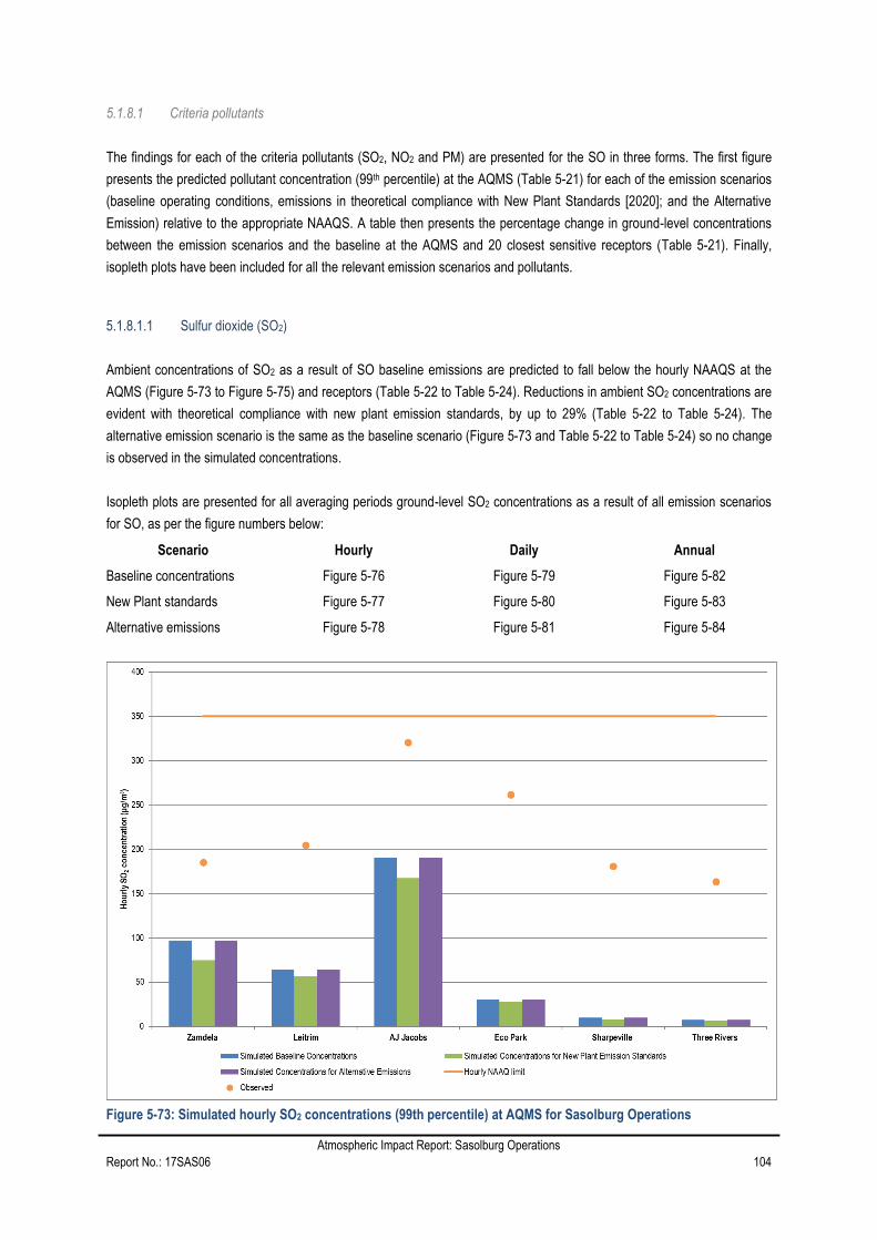
Atmospheric Impact Report: Sasolburg Operations
Report No.: 17SAS06 104
5.1.8.1 Criteria pollutants
The findings for each of the criteria pollutants (SO2, NO2 and PM) are presented for the SO in three forms. The first figure
presents the predicted pollutant concentration (99th percentile) at the AQMS (Table 5-21) for each of the emission scenarios
(baseline operating conditions, emissions in theoretical compliance with New Plant Standards [2020]; and the Alternative
Emission) relative to the appropriate NAAQS. A table then presents the percentage change in ground-level concentrations
between the emission scenarios and the baseline at the AQMS and 20 closest sensitive receptors (Table 5-21). Finally,
isopleth plots have been included for all the relevant emission scenarios and pollutants.
5.1.8.1.1 Sulfur dioxide (SO2)
Ambient concentrations of SO2 as a result of SO baseline emissions are predicted to fall below the hourly NAAQS at the
AQMS (Figure 5-73 to Figure 5-75) and receptors (Table 5-22 to Table 5-24). Reductions in ambient SO2 concentrations are
evident with theoretical compliance with new plant emission standards, by up to 29% (Table 5-22 to Table 5-24). The
alternative emission scenario is the same as the baseline scenario (Figure 5-73 and Table 5-22 to Table 5-24) so no change
is observed in the simulated concentrations.
Isopleth plots are presented for all averaging periods ground-level SO2 concentrations as a result of all emission scenarios
for SO, as per the figure numbers below:
Scenario Hourly Daily Annual
Baseline concentrations Figure 5-76 Figure 5-79 Figure 5-82
New Plant standards Figure 5-77 Figure 5-80 Figure 5-83
Alternative emissions Figure 5-78 Figure 5-81 Figure 5-84
Figure 5-73: Simulated hourly SO2 concentrations (99th percentile) at AQMS for Sasolburg Operations

Atmospheric Impact Report: Sasolburg Operations
Report No.: 17SAS06 105
Figure 5-74: Simulated daily SO2 concentrations (99th percentile) at AQMS for Sasolburg Operations
Figure 5-75: Simulated annual SO2 concentrations at AQMS for Sasolburg Operations

Atmospheric Impact Report: Sasolburg Operations
Report No.: 17SAS06 106
Table 5-22: Simulated baseline hourly SO2 concentrations and the theoretical change in concentrations relative to the baseline at the AQMs and 20 closest receptors
Receptor
Hourly SO2 (99th percentile)
Baseline New Alternative
Concentration (μg/m³)
Concentration (μg/m³)
Relative change Concentration
(μg/m³) Relative change
Zamdela AQMS 93.7 72.1 -23.1% 93.7 0%
Leitrim AQMS 62.7 56.4 -10.2% 62.7 0%
AJ Jacobs AQMS 167.7 141.0 -15.9% 167.7 0%
Eco Park AQMS 27.5 23.9 -13.1% 27.5 0%
Sharpeville AQMS 9.3 7.1 -24.0% 9.3 0%
Three Rivers AQMS 7.0 5.7 -17.5% 7.0 0%
Malakabeng Primary School 135.1 95.4 -29.3% 135.1 0%
Cedar Secondary School 86.1 72.6 -15.7% 86.1 0%
Bofula- Tshepe Primary School 90.4 70.7 -21.8% 90.4 0%
Clinic A Zamdela 95.3 73.8 -22.6% 95.3 0%
Zamdela Hospital Zumayear 117.1 84.0 -28.3% 117.1 0%
Iketsetseng Secondary School 90.4 70.7 -21.8% 90.4 0%
Clinic B Zamdela 77.7 67.5 -13.1% 77.7 0%
Tsatsi Primary School 152.6 102.6 -32.7% 152.6 0%
Isaac Mhlambi Primary School 77.5 66.8 -13.8% 77.5 0%
Nkopoleng Secondary School 115.9 81.6 -29.6% 115.9 0%
HTS Secondary School 188.5 146.3 -22.4% 188.5 0%
Zamdela Community Clinic 77.7 62.0 -20.1% 77.7 0%
AJ Jacobs Primary School 194.4 161.3 -17.0% 194.4 0%
Theha Setjhaba Primary School 72.2 59.1 -18.0% 72.2 0%
Sasolburg Clinic 150.9 126.0 -16.5% 150.9 0%
Credo Primary School 58.9 53.0 -9.9% 58.9 0%
Lehutso Primary School 66.2 53.9 -18.6% 66.2 0%
Harry Gwala Clinic | Creche 58.3 50.5 -13.3% 58.3 0%
Kahobotjha-Sakubusha Secondary School 104.5 83.8 -19.8% 104.5 0%
Sasolburg Provincial Hospital 50.1 42.6 -15.0% 50.1 0%

Atmospheric Impact Report: Sasolburg Operations
Report No.: 17SAS06 107
Table 5-23: Simulated baseline daily SO2 concentrations and the theoretical change in concentrations relative to the baseline at the AQMs and 20 closest receptors
Receptor
Daily SO2 (99th percentile)
Baseline New Alternative
Concentration (μg/m³)
Concentration (μg/m³)
Relative change Concentration
(μg/m³) Relative change
Zamdela AQMS 27.2 20.9 -23.2% 27.2 0%
Leitrim AQMS 16.2 14.5 -11.0% 16.2 0%
AJ Jacobs AQMS 63.2 51.9 -17.8% 63.2 0%
Eco Park AQMS 10.7 8.8 -17.7% 10.7 0%
Sharpeville AQMS 3.5 3.0 -15.5% 3.5 0%
Three Rivers AQMS 2.4 2.0 -16.5% 2.4 0%
Malakabeng Primary School 34.9 26.4 -24.5% 34.9 0%
Cedar Secondary School 26.1 22.0 -15.7% 26.1 0%
Bofula- Tshepe Primary School 26.2 20.5 -21.8% 26.2 0%
Clinic A Zamdela 27.9 21.1 -24.4% 27.9 0%
Zamdela Hospital Zumayear 30.1 23.0 -23.6% 30.1 0%
Iketsetseng Secondary School 26.2 20.5 -21.8% 26.2 0%
Clinic B Zamdela 21.5 19.2 -10.6% 21.5 0%
Tsatsi Primary School 38.1 28.0 -26.4% 38.1 0%
Isaac Mhlambi Primary School 22.8 19.3 -15.3% 22.8 0%
Nkopoleng Secondary School 29.5 22.1 -24.9% 29.5 0%
HTS Secondary School 54.4 41.1 -24.4% 54.4 0%
Zamdela Community Clinic 21.4 17.1 -20.2% 21.4 0%
AJ Jacobs Primary School 72.3 55.7 -23.0% 72.3 0%
Theha Setjhaba Primary School 20.1 16.1 -19.7% 20.1 0%
Sasolburg Clinic 47.4 40.4 -14.8% 47.4 0%
Credo Primary School 15.4 14.0 -8.8% 15.4 0%
Lehutso Primary School 18.1 14.5 -20.1% 18.1 0%
Harry Gwala Clinic | Creche 14.7 13.5 -8.1% 14.7 0%
Kahobotjha-Sakubusha Secondary School 42.8 35.5 -17.1% 42.8 0%
Sasolburg Provincial Hospital 16.0 13.5 -15.7% 16.0 0%
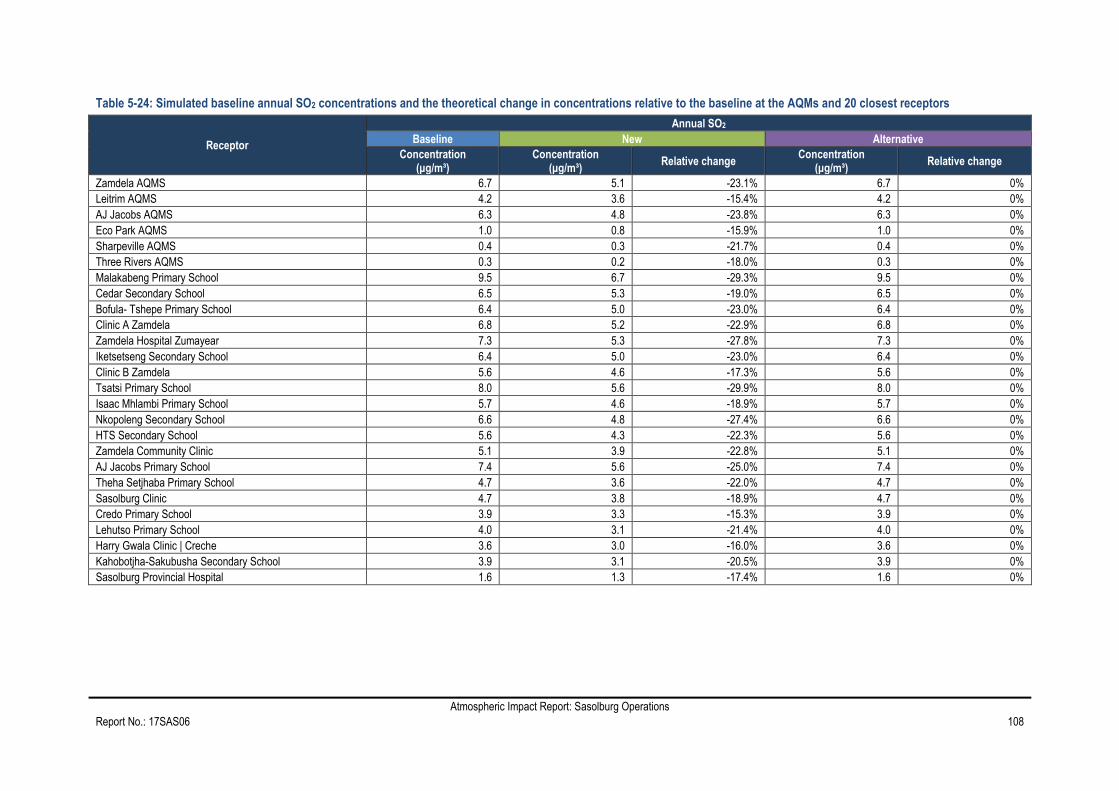
Atmospheric Impact Report: Sasolburg Operations
Report No.: 17SAS06 108
Table 5-24: Simulated baseline annual SO2 concentrations and the theoretical change in concentrations relative to the baseline at the AQMs and 20 closest receptors
Receptor
Annual SO2
Baseline New Alternative
Concentration (μg/m³)
Concentration (μg/m³)
Relative change Concentration
(μg/m³) Relative change
Zamdela AQMS 6.7 5.1 -23.1% 6.7 0%
Leitrim AQMS 4.2 3.6 -15.4% 4.2 0%
AJ Jacobs AQMS 6.3 4.8 -23.8% 6.3 0%
Eco Park AQMS 1.0 0.8 -15.9% 1.0 0%
Sharpeville AQMS 0.4 0.3 -21.7% 0.4 0%
Three Rivers AQMS 0.3 0.2 -18.0% 0.3 0%
Malakabeng Primary School 9.5 6.7 -29.3% 9.5 0%
Cedar Secondary School 6.5 5.3 -19.0% 6.5 0%
Bofula- Tshepe Primary School 6.4 5.0 -23.0% 6.4 0%
Clinic A Zamdela 6.8 5.2 -22.9% 6.8 0%
Zamdela Hospital Zumayear 7.3 5.3 -27.8% 7.3 0%
Iketsetseng Secondary School 6.4 5.0 -23.0% 6.4 0%
Clinic B Zamdela 5.6 4.6 -17.3% 5.6 0%
Tsatsi Primary School 8.0 5.6 -29.9% 8.0 0%
Isaac Mhlambi Primary School 5.7 4.6 -18.9% 5.7 0%
Nkopoleng Secondary School 6.6 4.8 -27.4% 6.6 0%
HTS Secondary School 5.6 4.3 -22.3% 5.6 0%
Zamdela Community Clinic 5.1 3.9 -22.8% 5.1 0%
AJ Jacobs Primary School 7.4 5.6 -25.0% 7.4 0%
Theha Setjhaba Primary School 4.7 3.6 -22.0% 4.7 0%
Sasolburg Clinic 4.7 3.8 -18.9% 4.7 0%
Credo Primary School 3.9 3.3 -15.3% 3.9 0%
Lehutso Primary School 4.0 3.1 -21.4% 4.0 0%
Harry Gwala Clinic | Creche 3.6 3.0 -16.0% 3.6 0%
Kahobotjha-Sakubusha Secondary School 3.9 3.1 -20.5% 3.9 0%
Sasolburg Provincial Hospital 1.6 1.3 -17.4% 1.6 0%