Available in: http://www.redalyc.org/articulo.oa?id=57137208

Red de Revistas Científicas de América Latina, el Caribe, España y Portugal

Sistema de Información Científica

W. J. Schuster, L. Parrao

The Atmospheric Extinction of San Pedro Mártir W. J. Schuster & L. Parrao

Revista Mexicana de Astronomía y Astrofísica, vol. 37, núm. 2, octubre, 2001, pp. 187-200,

Instituto de Astronomía

México

How to cite Complete issue More information about this article Journal's homepage

Revista Mexicana de Astronomía y Astrofísica,

ISSN (Printed Version): 0185-1101

rmaa@astroscu.unam.mx

Instituto de Astronomía

México

www.redalyc.orgNon-Profit Academic Project, developed under the Open Acces Initiative

© C

op

yrig

ht 2

001:

Inst

ituto

de

Ast

rono

mía

, Uni

vers

ida

d N

ac

iona

l Aut

óno

ma

de

Mé

xic

o

Revista Mexicana de Astronomıa y Astrofısica, 37, 187–200 (2001)

THE ATMOSPHERIC EXTINCTION OF SAN PEDRO MARTIR1

W. J. Schuster2 and L. Parrao3

Received 2001 April 6; accepted 2001 July 9

RESUMEN

Se analiza la extincion atmosferica de San Pedro Martir (SPM) utilizandodeterminaciones en 13 colores de 294 noches de observacion durante los anos de1973–1983, ademas de mediciones de extincion para 272 noches de observacionen uvby durante los anos 1984–1999. Se obtiene el comportamiento general dela extincion normal en SPM, y se analiza este como funcion de la longitud deonda y del tiempo; se aportan valores promedio y mınimos para esta extincion.La extincion atmosferica promedio en SPM, excluyendo erupciones volcanicas, nocambio apreciablemente durante el perıodo 1973–1999. Se presenta un modelosencillo, de tres componentes, para la extincion en SPM. Los aerosoles normales,promedio, no volcanicos sobre SPM se ajustan bien por kp(λ) = 0.0254(λ)−0.87. Sepresentan las determinaciones de la extincion para los perıodos que siguieron a laserupciones de los volcanes de El Chichon y el Pinatubo: los datos en 13 coloresmuestran los efectos de El Chichon, y los datos uvby los del Pinatubo. Se analizanlas curvas de extincion y sus variaciones para estudiar los aerosoles volcanicos ysu evolucion en el tiempo. Se estudia tambien la temporada de observacion deabril y mayo de 1998, en la cual ocurrieron grandes variaciones no volcanicas en laextincion, y se presentan deducciones sobre estos aerosoles inusuales.

ABSTRACT

The atmospheric extinction of San Pedro Martir (SPM) is analyzed using 13-color determinations from 294 nights of observations over the years 1973–1983, plusthe extinction measures from 272 nights of uvby observations over the years 1984–1999. The general behavior of the normal extinction at SPM is given and analyzedas a function of wavelength and as a function of time. The average atmosphericextinction at SPM, excluding volcanic outbursts, has not changed significantly overthe period 1973–1999. A simple 3-component model for the extinction above SPMis derived and presented; the normal, average, non-volcanic aerosols above SPMare well fit by kp(λ) = 0.0254λ−0.87. The extinction determinations for the periodsfollowing the volcanoes El Chichon and Pinatubo are given: 13C data show theeffects of El Chichon and uvby for Pinatubo. The extinction curves and theirvariations are analyzed to study the volcanic aerosols and their evolution withtime. The Apr/May’98 observing run, when large non-volcanic extinction variationsoccurred, is also studied and deductions drawn concerning these unusual aerosols.

Key Words: ATMOSPHERIC EXTINCTION — ATMOSPHERES: TER-

RESTRIAL — TECHNIQUES: PHOTOMETRIC

1Based on observations collected at the Observatorio As-

tronomico Nacional at San Pedro Martir, Baja California,

Mexico.2Instituto de Astronomıa and Observatorio Astronomico

Nacional, UNAM, Ensenada, B. C.3Instituto de Astronomıa, Universidad Nacional Auto-

noma de Mexico.

187

© C

op

yrig

ht 2

001:

Inst

ituto

de

Ast

rono

mía

, Uni

vers

ida

d N

ac

iona

l Aut

óno

ma

de

Mé

xic

o

188 SCHUSTER & PARRAO

1. INTRODUCTION

Since its beginnings in 1968, stellar photometryhas played a very important role in the develop-ment of the Mexican National Astronomical Obser-vatory at San Pedro Martir, Baja California, Mexico(hereafter SPM). Some of the very first astronomicalequipment on this mountain were stellar photome-ters, such as one of the original Johnson UBVRIphotometers and also the 13-color, 8C and 6RC, pho-tometers of Johnson, Mitchell, & Latham (1967)and of Mitchell & Johnson (1970). Later the Low-ell pulse counting photometers were acquired as wellas rapid and dual-channel photometers. The “Dan-ish” 6-channel uvby-β photometer arrived near theend of 1983 and has played a key part in many ofthe photometric programs at this observatory. Overthe last few years CCD detectors have replaced inpart these classical photometers for the observationof stellar objects, especially for extended ones suchas open and globular clusters. However, much ofthe most precise, accurate, and well-calibrated stel-lar photometry is still being carried out at SPMwith the classical photometers such as the “Dan-ish”. Several important projects and surveys haveresulted, such as those concerning variable stars(Gonzalez-Bedolla 1990), subdwarf, metal-poor andhigh-velocity stars (Schuster & Nissen 1988; Schus-ter, Parrao, & Contreras-Martınez 1993), and alsopre-main-sequence objects (Chavarrıa et al. 1988;2000).

The SPM observatory has been characterized inseveral previous publications, such as the prelimi-nary report of Mendoza (1971), and the climatolog-ical and meteorological studies of Alvarez & Mais-terrena (1977) and of Tapia (1992). Astronomi-cal seeing at SPM has been evaluated in works byWalker (1971) and Echevarria et al. (1998). Theprecipitable water vapor above SPM has been de-termined and analyzed by Hiriart et al. (1997) andthe turbulence profiles above the 1.5 m and 2.1 mtelescopes by Avila, Vernin, & Cuevas (1998). Pre-vious studies of the atmospheric extinction at SPMhave been published by Schuster (1982), (hereafterS82) and by Schuster & Guichard (1985), (hereafterSG). In the former the 13-color photometric systemwas used to study the atmospheric extinction as afunction of wavelength and of time. The extinctioncurve versus λ was given from 212 nights of nor-mal observations, plus the curves from two specialextinction nights observed to large air masses withthe participation of M. Alvarez. Year to year vari-ations, monthly averages and an overall mean werepresented. The atmospheric extinction of SPM was

compared to that of 23 other astronomical observato-ries, that of SPM being the second lowest, surpassedonly by Mauna Kea, Hawaii. The extinction curveand its variations were assessed in terms of the windand rainfall patterns of this observatory; northernwinds, for example, bring higher extinctions due tourban and dust pollutants from the north. In SGmore yearly means were given as well as the extinc-tion curve versus wavelength for normal conditionsand for the two years following the El Chichon vol-cano in 1982. Arguments were made for a possiblebi-modal distribution of aerosols following this vol-cano, for the masking of the usual ozone absorptionnear 5800 A, and for additional absorption at the 37filter due to the SO2 molecule.

In the present study the atmospheric extinctionof SPM is reanalyzed using the 13-color (hereafter13C) results from 294 nights of observations over theyears 1973–1983, plus the extinction determinationsfrom 272 nights of uvby-β observations over the years1984–1999. In § 2 the observing techniques used forthe extinction determinations are discussed briefly.In § 3 the general behavior of the normal extinctionat SPM is given and analyzed as a function of wave-length and as a function of time. Mean and minimumatmospheric extinction values for SPM are given. In§ 4 a simple 3-component model for the extinctionabove SPM is derived and presented; this model in-cludes Rayleigh and aerosol scattering plus ozone ab-sorption and fits the observed extinction curve wellover 3370–6500 A. In § 5 the extinction determi-nations for the periods following the volcanoes ElChichon and Pinatubo are given, 13C data for theeffects of El Chichon and uvby for Pinatubo. Theextinction changes and variations are analyzed tostudy the volcanic aerosols and their evolution withtime, and to detect possible masking of the usualextinction components. The Apr/May’98 observingrun, when large non-volcanic extinction variationsoccurred, is also studied, and deductions drawn con-cerning the climatological conditions and their un-usual aerosols. Our conclusions are given in § 6.

2. OBSERVING TECHNIQUES

The 13C extinction determinations were madewith the single-channel 8C and 6RC photometers de-scribed in S82 and SG. Briefly, the Bouguer methodfor the determination of the atmospheric extinctioncoefficients has been employed. Usually one extinc-tion pair, including one red and one blue star, nearthe celestial equator, was observed three times, atsmall, intermediate, and large air masses. Infre-quently, two extinction pairs were observed, eachat small and large air masses. For each case an

© C

op

yrig

ht 2

001:

Inst

ituto

de

Ast

rono

mía

, Uni

vers

ida

d N

ac

iona

l Aut

óno

ma

de

Mé

xic

o

THE ATMOSPHERIC EXTINCTION OF SAN PEDRO MARTIR 189

air mass range of at least 0.8 was required for theextinction solution. Being single-channel photome-ters the observations were fairly slow, and so usuallyless than 15 standard stars (including the extinctionstars) were observed per night. Although each ex-tinction pair contained both a red and blue star, nosecond-order extinction terms were needed, exceptperhaps a very small one for the 33 filter, which hasbeen ignored.

The 4-color extinction determinations were madeusing the uvby-β, 6-channel photometer on SPM atthe 1.5 m H.L. Johnson telescope. More details con-cerning our observing techniques can be found inSchuster & Nissen (1988) and Grønbech, Olsen,& Stromgren (1976). Tests have shown that thesecond-order extinction term in c1 is less than 0.m002,and so it has been ignored. So, extinction pairs havebeen retained here not for the second-order term butfor the greater precision provided; these pairs usuallycontained F- and G-type standard stars, similar toour metal-poor program stars. Again they were lo-cated near the celestial equator for optimal efficiencyand precision. The Bouguer method has again beenused, and usually the air-mass range of the extinc-tion determinations was greater than 0.8. If the pairwas well centered during the night, it was observed 5times: ∼> 4.0 and 2.5–2.0 hours east of the meridian,then crossing the meridian, and finally 2.0–2.5 and

∼> 4.0 hours west. If the pair was not so well centered,only four observations of the pair were obtained witha single observation at ∼ 3.0 hours substituted, eastor west, depending on the centering.

All the observations were reduced using Fortranprograms graciously provided by T. Andersen andP.E. Nissen, and these are documented in Parrao,Schuster, & Arellano-Ferro (1988) and follow closelythe precepts of Grønbech et al. (1976). All nightsof an observing run are reduced together to providean instrumental photometric system. The output ofthe reduction provides nightly extinction coefficientstogether with their error estimates as well as the con-stant and temporal terms of the night correction foreach night, as defined by Grønbech et al. (1976).The linear-time terms of the night corrections de-pend upon the observations of “drift” stars observedsymmetrically east and west of the meridian; theseare stars with more northerly declinations (∼> +20◦).Typical (median) estimated errors for the extinctioncoefficients of y, (b−y), m1, c1 are ± 0.0030, 0.0016,0.0025, and 0.0.0030. The program also outputsnightly scatters to help us evaluate the photomet-ric quality of the nights.

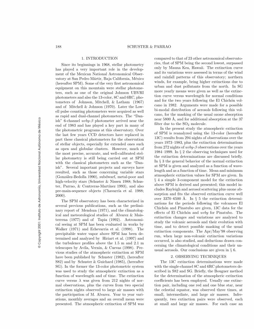
4000 6000 80000

0.2

0.4

0.6

0.8

Pinatubo, uvby maximum

13-color average

uvby minimum

uvby average

El Chichon, 13C maximum

Fig. 1. Atmospheric extinction versus the equiv-alent wavelengths of the 13C and 4-color filters.Solid squares and circles show the average extinctionsfrom 151(8C)/120(6RC) nights of 13C photometry and158(mags.)/182(colors) nights of 4-color photometry, re-spectively. The lowest curve shows the “minimum” 4-color extinction as derived from 12 nights with opti-mal, stable conditions from 6 good observing runs from1988 through 1998. These mean and minimum valuesare shown in Table 1. The highest curves of this graphshow the maximum effects caused by volcanic aerosols,the night of 19/20 Jun’82 for 13C photometry and theEl Chichon volcano (open squares), and the night of 4/5May’92 for 4-colors and Pinatubo (open circles).

3. BEHAVIOR OF THE ATMOSPHERICEXTINCTION AT SPM

3.1. As a Function of Wavelength

In Figure 1 are shown the mean and extremeatmospheric extinctions observed at SPM over theyears 1973 through 1999 with the 13C and 4-colorphotometry. The extinction values are plotted ver-sus the equivalent wavelengths of the photometricband passes. For 13C these wavelengths have beentaken from Mitchell & Johnson (1970). For the 4-color photometry the equivalent wavelengths havebeen taken from the manual of Nissen (1984) with asmall correction to the “u” wavelength according tothe new atmospheric extinction model of this paper(see § 4 below). For 4-color photometry the equiv-alent wavelengths used here are: 3515, 4110, 4685,and 5488 A. Fig. 1 shows the mean 13C extinctioncurve for 271 nights of 8C and 6RC photometry over

© C

op

yrig

ht 2

001:

Inst

ituto

de

Ast

rono

mía

, Uni

vers

ida

d N

ac

iona

l Aut

óno

ma

de

Mé

xic

o

190 SCHUSTER & PARRAO

the years 1973–1981, prior to the El Chichon volcanoand its strong effects on the atmospheric extinction.151 nights of 8C and 120 of 6RC photometry go intothis average 13C curve. Also shown is the mean 4-color extinction curve for the period 1984–1999 withthe observations from Oct’91 through Apr’94 omit-ted due to the effects of the Pinatubo volcano. Forthis “uvby average” curve 182 nights define the shapeof the curve while only 158 nights the level. As dis-cussed in Schuster & Nissen (1988) a small subset ofour observations have been made through light cir-rus clouds in the absence of moonlight; observationsmade with the simultaneous multichannel photome-ter provide good color and index data through lightclouds, but not good magnitudes. Also plotted inFig. 1 is a “uvby minimum” curve which representsthe average of 12 nights with the lowest extinctiondeterminations from six observing runs with the low-est average extinctions and most stable observingconditions: Jun’88, Nov’89, Oct’94, Oct’97, Nov’97,and Nov’98. The average of 12 nights is given here topresent a value which is robust and representative.

In Table 1 are shown the mean and minimum ex-tinction coefficients observed at SPM for the 13C and4-color photometry as shown in Fig. 1; for the 4-colorresults both the observed color and index extinctionsare given with their dispersions (of a single measure),as well as the extinctions converted to magnitude val-ues. The “mean” four-color values exclude the datesaffected by Pinatubo, and the “minimum” values usethe 12 nights from the 6 stable observing runs men-tioned above. The 13-color averages cover the years1973–1981.

Also plotted in Fig. 1 are the most extreme ex-tinctions observed at SPM by us using the 13C and 4-color photometers. The 13C maximum occurred forthe period following the El Chichon volcanic erup-tion. The level and blue part of this curve are definedby a single night, the 19/20th of Jun’82, while thered part of this curve includes 6RC data from sev-eral nights during 1982 following the eruption. The“uvby maximum” curve comes from the observationsof a single night, 4/5 May’92, during the maximumeffects at SPM due to the Pinatubo volcano.

The average 13C extinction curve of Fig. 1shows the expected shape over the wavelength range3370–11,080 A with Rayleigh and aerosol scatteringplus ozone absorption dominating over 3370–6500 Aand additional absorptions by O2 and H2O forλ ∼> 6500 A (Cox 2000, Fig. 11-4). Also this 13Ccurve of Fig. 1 shows a bump at the 58 filter whichis probably evidence for the Chappuis bands ofozone; the strongest absorptions of the Chappuis

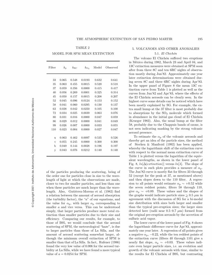
TABLE 1

OBSERVED EXTINCTION AT SPM

Four ColorColor: y (b − y) m1 c1 N

Mean +0.140 +0.057 +0.047 +0.122 158/182

±0.030 ±0.006 ±0.008 ±0.009

Min +0.112 +0.056 +0.044 +0.122 12

±0.002 ±0.004 ±0.007 ±0.010

Filter: u v b y N

Mean 0.526 0.300 0.197 0.140 158/182

Min 0.491 0.268 0.168 0.112 12

13-ColorFilter 33 35 37 40 N(8C)

Mean 0.641 0.518 0.417 0.314 151

Filter 45 52 58 63 N(8C)

Mean 0.207 0.152 0.137 0.100 151

Filter 72 80 86 99 110 N(6RC)

Mean 0.076 0.059 0.049 0.055 0.047 120

bands occur over the wavelengths 5650–6250 A(Gast 1961) . The two “average” curves of Fig. 1 arein very good agreement indicating that the meanatmospheric extinction of SPM has not evolvedsignificantly, outside of the volcanic episodes, fromthe 1973–1981 period through 1984–1999. Forexample, the mean visual extinction (filters 52 and58) from 13C was 0.m144 per air mass from 151nights of 8C observations and 0.m140 per air massfrom 158 nights of 4-color determinations. The“minimum” curve shows kV ∼ 0.m11 per air mass,which compares very favorably with that of manyother observatories (S82); Burki et al. (1995),(hereafter B95) obtained a minimum of kV ∼ 0.m13from about 4,400 nights of photometry at the LaSilla, Chile, observatory using the seven bands ofthe Geneva photometric system.

© C

op

yrig

ht 2

001:

Inst

ituto

de

Ast

rono

mía

, Uni

vers

ida

d N

ac

iona

l Aut

óno

ma

de

Mé

xic

o

THE ATMOSPHERIC EXTINCTION OF SAN PEDRO MARTIR 191

The two extreme curves of Fig. 1 show similarlevels for the two volcanoes. These extrema also giveus the first indications for the differing and unusualwavelength dependences for the volcanic aerosols(see § 5 below); the El Chichon curve has an upwardshift from the mean of 0.m221 in the ultraviolet (filter35) and 0.m214 in the visible (filters 52 and 58), whilethe Pinatubo curve is displaced 0.m162 and 0.m198 inthe UV and visible, respectively.

3.2. As a Function of Time

Figure 2 shows the variation of ky at SPM fromthe end of 1984 through 1999, determined with theuvby-β photometer. In the upper graph the averagevalues plus error bars are shown for 33 different ob-serving runs, as a function of the civil calendar; inthe middle panel the ky values are plotted for nightlyvalues as a function of the Julian date. The trian-gles show our extinction values as measured accord-ing to the methods and techniques discussed in § 2.The filled squares show extinction data measuredand graciously provided by other observers, suchas S. Gonzalez-Bedolla, A. Ruelas-Mayorga, J. H.Pena, and A. Arellano-Ferro; these are plotted herefor completeness and better coverage, but are notused for the modeling and analyses to follow due tothe differing observing and reduction methods em-ployed. The upper horizontal bar marks the inter-val of observations affected by the volcanic aerosolsfrom Pinatubo, Julian dates about 2448400–9500,including the Oct’91, Mar’92, Apr/May’92, Nov’92,Mar’93, May’93, Sep’93, Nov’93, and Apr’94 observ-ing runs. Large variations and instability are alsonoted for the Apr/May’98 observing run (and alsofor Feb’85 and May’89), not caused by any volcanicactivity; this behavior will be discussed in § 5.3.

In the lower panel of Fig. 2 five expanded plotsare shown for five of the observing runs; four ofthese, Oct’91, Mar’92, Apr/May’92, and Nov’92,were clearly affected by the Pinatubo aerosols, andthe fifth, the first run of the Apr/May’98 period, wasextinguished by some sort of significant non-volcanicabsorption. The Pinatubo plots, especially the onesfor Oct’91 and Apr/May’92, show evidence for thestriations and patchiness of the volcanic aerosols ashas been detected and discussed in other works, suchas Stothers (2001). On the other hand, the ex-panded plot for the Apr/May’98 run shows clearevidence for a single event or aerosol cloud havingpassed over SPM, with its maximum effect happen-ing during the night of 26/27 Apr’98.

0.1

0.2

0.3

0.4

J.D.(2,400,000.+)

1985 1990 1995

0.1

0.2

0.3

0.4

YEAR

0.1

0.2

0.3

0.4

Fig. 2. In the upper panel the average atmospheric ex-tinction values for the “y” band are plotted with theirdispersions as a function of the civil calendar for 33 ob-serving runs from Oct’84 through Apr’99. The intervalprobably affected by the volcanic aerosols from Pinatubois indicated. Triangles show values measured by us, whilefilled squares values measured by others. The middlepanel shows the same, but for the nightly individual val-ues, as a function of the Julian dates. The Apr/May’98period, which showed a large, non-volcanic variation inthe atmospheric extinction, is also labeled. The bottompanel displays expanded plots for five of the observingruns, four affected by the Pinatubo aerosols and the firstobserving run of the Apr/May’98 period.

In Figure 3 the extinction coefficients for y,(b − y), m1, and c1 are plotted as a function of themonth of the year. The data affected by Pinatubohave been excluded. It can be seen that the largerextinction excursions for SPM generally occur for thespring months of March–May while the fall monthsare more stable; this had been noted by S82 from13C extinction data. This latter result can also beappreciated from the list of observing runs used forthe “minimum” curve of Fig. 1; five out of six were inOctober or November. This Fig. 3 can be contrastedwith Figure 6 of B95 where the largest extinction ex-cursions happen at La Silla during the southern sum-mer months; during the summer the reversing layeris sometimes above La Silla. The explanation forSPM is not so obvious. According to Tapia (1992),May is the month with the highest percentage ofphotometric nights at SPM, while April and Mayare the two months with the highest percentages of

© C

op

yrig

ht 2

001:

Inst

ituto

de

Ast

rono

mía

, Uni

vers

ida

d N

ac

iona

l Aut

óno

ma

de

Mé

xic

o

192 SCHUSTER & PARRAO

nights with high relative humidity. Large meteoro-logical aerosols, i.e., “haze” (water droplets), mayhave caused the higher atmospheric extinctions. OnSPM the costal or local inversion layers probably donot reverse or break down during such episodes (Al-varez & Maisterrena 1977). And, as the discussion of§ 5.3 shows, wind direction may also play an impor-tant role. It is curious that Echevarrıa et al. (1998)obtained better seeing results at SPM for the springand summer months and poorer for the autumn andwinter; perhaps the higher humidities of the spring(Tapia 1992) promote better seeing but at the sametime larger meteorological aerosols with higher andless stable atmospheric extinctions. More completemeteorological data are needed for SPM.

4. A THREE-COMPONENT MODEL FOR THEATMOSPHERIC EXTINCTION OF SPM.

4.1. The Model

The atmospheric extinction model developed inthis section follows closely the physics and for-mulism given in papers such as B95, Gutierrez-Moreno, Moreno, & Cortes (1982), and Hayes &Latham (1975). It assumes that the extinction over3200 ∼< λ ∼< 6500 A can be represented by three in-dependent contributions due to Rayleigh-Cabannesand aerosol scatterings and ozone absorption

k(λ) = kp(λ) + kRC(λ) + kO3(λ),

= aλ−αp + bλ−4.05 + ckoz(λ), (1)

where kp(λ) represents the aerosol term given byaλ−αp ; kRC(λ) is the Rayleigh-Cabannes componentgiven by bλ−4.05, where the exponent of −4.05 hasbeen taken from Allen (1973) and includes approx-imately the refractive effects; and kO3

(λ), the ozonecontribution given by ckoz(λ). For the normalizationof this model, the Rayleigh-Cabannes coefficient “b”is calculated to be 0.0067 according to equation (1) ofHayes & Latham (1975), using an altitude of 2790 mfor the 1.5 m telescope on SPM and assuming a den-sity scale height of 7.996 km for the lower tropo-sphere (Hayes & Latham 1975). This normalizationcorresponds to standard conditions, and variationsin barometric pressure may cause uncertainties ofabout one percent. For the ozone term, equation (2)of Hayes & Latham (1975) has been adapted so thatc = 1.11 Toz where Toz can be taken from § 59 ofAllen (1963) according to the latitude of SPM andaccording to the months when most of our obser-vations were taken. We find Toz ∼ 0.2325 givingc ∼ 0.2581. The values of koz(λ) can be obtainedfrom Gast (1961), (Tables 16–16B and 16–16C) byconvolving his ozone data with the filter sensitiv-

0.1

0.15

0.2

0.25

0.3

MONTH

Jan. April July Oct. Jan.

0.02

0.04

0.06

0.08

0.1

0.02

0.04

0.06

0.08

0.1

0.1

0.12

0.14

0.16

Fig. 3. The atmospheric extinctions for c1, m1, (b − y),and y are plotted versus the months of their observationin order to detect and study the seasonal and annualvariations. The data affected by the aerosols from thePinatubo volcano have been removed from this plot.

ity functions, from Grønbech et al. (1976) for theuvby system and from Johnson et al. (1967) andMitchell & Johnson (1970) for 13C. The ozone data(Gast 1961) given for a temperature of −44◦C wereused whenever possible corresponding to altitudesof 10 to 35 km, where most of the pertinent at-mospheric ozone is concentrated. Since the ozoneabsorption can be quite variable (Hayes & Latham1975), these ozone extinction values provide us onlywith the means of studying the average atmosphericextinction above SPM.

The aerosol contribution can now be studied bysubtracting the Rayleigh-Cabannes and ozone ex-tinctions from the total observed extinction

kp(λ) = k(λ) − kRC(λ) − kO3(λ) = aλ−αp . (2)

This equation must now be solved for a and −αp us-ing our observed mean extinction data. A methodsimilar to that of B95 is used here for our 4-colordata. Regressions of kp(λu), kp(λv), and kp(λy)against kp(λb) have been made, with the mean min-imum extinctions of Table 1 subtracted; these rela-tions are shown in Figure 4. Here we are mainlyconcerned with normal, average conditions aboveSPM, and so the data affected by Pinatubo andthe data of the unstable observing runs such asMay’89 and Apr/May’98 have been removed from

© C

op

yrig

ht 2

001:

Inst

ituto

de

Ast

rono

mía

, Uni

vers

ida

d N

ac

iona

l Aut

óno

ma

de

Mé

xic

o

THE ATMOSPHERIC EXTINCTION OF SAN PEDRO MARTIR 193

0

0.05

0.1

0

0.05

0.1

Fig. 4. The kp(u), kp(v), and kp(y) versus kp(b) plotsfor 138 nights of extinction data. Data affected byPinatubo and data from the less stable Apr/May’98 andMay’89 observing runs have been removed. Regressionsto this data give the extinction ratios to be used in thelog[kp(λi)/kp(λb)] versus log[λi/λb] method as discussedin the text and shown in the following graph. The regres-sions shown here have slopes of 1.265 for kp(u), 1.134 forkp(v), and 0.861 for kp(y).

the analyses leaving 138 nights of uvby data. Theresults of these regressions are then plotted in theform, log[kp(λi)/kp(λb)] versus log[λi/λb], as shownin Figure 5. A regression of this graph then gives αp.For normal, average conditions on SPM, αp = 0.87±0.04 is obtained. Then equation (2) can be used toderive the turbidity factor “a”. For 13C the filters33 through 63 give, < a >33−63= 0.02524± 0.00308;the 13C filters 72 through 110 are not used here sincethey are probably affected by other absorption com-ponents (Cox 2000). For the 4-color results the “u”calculation does not agree that well with the valuesfrom “vby”, probably due to still some uncertaintyin its equivalent wavelength, which is magnified bythe steeply increasing Rayleigh-Cabannes dispersionfor this filter. The other three 4-color measures ofextinction give, < a >= 0.02547 ± 0.00020, whichagrees well with the 13C result. Inverting the processwould imply an equivalent wavelength for the “u”band of 3533 A, as compared to our given 3515 A,the difference being well within this band’s uncer-tainty. So the normal mean aerosols above SPM canbe represented by

-0.15 -0.1 -0.05 0 0.05 0.1

-0.1

0

0.1

0.2

Fig. 5. The log[kp(λi)/kp(λb) versus log[λi/λb] graphfor determining the αp exponent of the normal, aver-age aerosol extinction above SPM. The regression whichis shown by filled circles corresponds to the slopes ofFig. 4 and gives αp = 0.87 ± 0.04, so that the ex-tinction law for the average, normal aerosols is of theform kp(λ) = aλ−0.87. Also shown is the slope for themost negative αp found during the Apr/May’92 observ-ing run, which was hightly affected by the Pinatubo vol-canic aerosols (see Fig. 9 below); the nearly neutral slopeobtained during the Apr/May’98 run (+0.28±0.04), dis-cussed in § 5.3; and the curve with the most positive αp

(+1.67 ± 0.04), for the Aug’97 observations, indicatingsome of the smallest aerosol particles above SPM.

kp(λ) = aλ−αp = 0.0254λ−0.87,

and our total model by

k(λ) = 0.0254λ−0.87 + 0.0067λ−4.05 + 0.2581koz(λ), (3)

where λ is measured in microns. In Table 2 are pre-sented the extinction values for these three compo-nents, plus the summed model and observed extinc-tions, for the 4-color and 13C photometry.

In Figures 6 and 7 are shown the components ofour 3-component model for the atmospheric extinc-tion over SPM and the fits of this model to our meanextinctions for the 13C and 4-color photometry. Theupper panel of Fig. 6 shows the individual contribu-tions of Rayleigh and aerosol scatterings and ozoneabsorption within the bands of the 13C system, plusthe observed mean extinction for 13C and the modelshifted upward by 0.05 for comparison. The lowerpanel shows the fit of the model to the observed

© C

op

yrig

ht 2

001:

Inst

ituto

de

Ast

rono

mía

, Uni

vers

ida

d N

ac

iona

l Aut

óno

ma

de

Mé

xic

o

194 SCHUSTER & PARRAO

0

0.2

0.4

0.6

Rayleigh3-component model

plus 0.05Obs.Aerosols

Ozone

4000 6000 8000

0

0.2

0.4

0.6

Difference

3-component model

Obs.

Obs.

Wavelength (A)

Fig. 6. The upper panel of this figure shows the threecomponents of our simple extinction model for SPM inthe 13C photometric system, plus the mean 13C extinc-tion of SPM from Table 1, and finally the sum of the threecomponents shifted upward by 0.05 for clarity and com-parison. Open squares represent the ozone contributionfor SPM, open triangles the aerosol contribution, opencircles the Rayleigh-Cabannes, filled circles the mean ob-served extinction, and asterisks the shifted model. In thelower panel the observed-mean and model extinctions areover-plotted, and below the residuals (obs.−model) areplotted as filled triangles, all as a function of the equiv-alent wavelengths of the 13C filters. The model fits theobserved curve very well for 3700–6500 A but falls shortfor greater wavelengths due to the lack of absorptions byO2 and by H2O.

mean extinction, and at the bottom the residualsof this fit, all as a function of the equivalent wave-lengths. Fig. 7 shows the same for the 4-color systemand its mean atmospheric extinction above SPM.The mean residual of the lower panel of Fig. 6 is< ∆obs−model >= −0.m0002±0.m0061 for the fit of thefilters 33 through 63, using a = 0.0254, and for thelower part of Fig. 7 for 4-colors, < ∆obs−model >=−0.m0022 ± 0.m0047, including all four bands. Themean residual of Fig. 7 for the “vby” bands is <∆obs−model >= +0.m0001± 0.m0004. In Fig. 6 it canbe seen that the 3-component model falls short forwavelengths greater than 6500 A, for the filters 72through 110. This is what one would expect fromthe data plotted in Fig. 11-4 of Cox (2000); thereare additional absorptions by O2 and by H2O forthese longer wavelengths, and so our 3-component

0

0.2

0.4

0.6

Rayleigh

Obs.

Aerosols

Ozone

3-component model plus 0.05

3500 4000 4500 5000 5500

0

0.2

0.4Obs.

Difference

3-component model

Wavelength (A)

Fig. 7. The same as Fig. 6, but for the 4-color, uvby,photometric system.

model is no longer complete.

4.2. Comparisons with other Observatories

Our value for the exponent of the aerosol scatter-ing can be compared to that for other observatories.For example, B95 obtain kp(λ) = aλ−1.39 for LaSilla, Chile, from about 4,400 nights using theGeneva photometric system, and they commentthat values close to this, −1.3 ± 0.2, are found“...at a large variety of locations on the Earth...being seldom above −0.5 or below −1.6.” However,Gutierrez-Moreno et al. (1982) find values of αp

varying from 0.2 to 2.6 from a large data set ofmonochromatic extinction determinations made atthe Cerro Tololo Inter-American Observatory, Chile,from 1964 to 1980. Hayes & Latham (1975) findvalues from 0.49 to 0.89 for stellar observations atseveral observatories, such as Le Houga, Boyden,Lick, Cerro Tololo, and Mount Hopkins. Theyfind a mean weighted value of 0.81 for their stellarobservations and adopt αp = 0.8 for nighttimestellar photometry, very close to the value that wehave obtained for SPM. They comment, “this valueis smaller than those quoted in the literature onatmospheric aerosols, which usually refer to loweraltitudes and poorer transparency conditions, suchas are found near urban centers.”

As discussed in many of the above references,this aerosol exponent is closely related to the sizes

© C

op

yrig

ht 2

001:

Inst

ituto

de

Ast

rono

mía

, Uni

vers

ida

d N

ac

iona

l Aut

óno

ma

de

Mé

xic

o

THE ATMOSPHERIC EXTINCTION OF SAN PEDRO MARTIR 195

TABLE 2

MODEL FOR SPM MEAN EXTINCTION

Filter kp kRC kO3 Model Observed

33 0.065 0.548 0.0193 0.632 0.641

35 0.063 0.455 0.0015 0.520 0.518

37 0.059 0.356 0.0000 0.415 0.417

40 0.056 0.269 0.0001 0.325 0.314

45 0.050 0.157 0.0015 0.208 0.207

52 0.045 0.096 0.0124 0.153 0.152

58 0.041 0.060 0.0295 0.130 0.137

63 0.038 0.042 0.0250 0.105 0.100

72 0.034 0.025 0.0039 0.063 0.076

80 0.031 0.016 0.0000 0.047 0.059

86 0.029 0.012 0.0000 0.041 0.049

99 0.026 0.007 0.0000 0.033 0.055

110 0.023 0.004 0.0000 0.027 0.047

u 0.063 0.462 0.0097 0.535 0.526

v 0.055 0.245 0.0000 0.300 0.300

b 0.049 0.144 0.0028 0.196 0.197

y 0.043 0.076 0.0212 0.140 0.140

of the particles producing the scattering, being ofthe order one for particles close in size to the wave-length of light at which the observations are made,closer to two for smaller particles, and less than onewhen these particles are much larger than the wave-length. Also, Gutierrez-Moreno et al. (1982) finda relation between the amount of aerosol absorption(the turbidity factor), the “a” of our equations, andthe value for αp, with larger αp corresponding tosmaller a and vice versa. This can be understoodsimply, that larger particles produce more total ex-tinction than smaller particles due to their size andefficiency. Comparing our results, for example, tothose of B95, we would conclude that the aerosolscattering of SPM, the meteorological “haze”, is dueto larger particles than those of La Silla, and theamount of aerosol scattering somewhat larger, al-though the minimum overall extinction of SPM issmaller than that of La Silla. In fact, Rufener (1986)found the very low value of 0.006 for the aerosol tur-bidity at La Silla, while we have found a more typicalvalue of a = 0.0254 for SPM.

5. VOLCANOES AND OTHER ANOMALIES

5.1. El Chichon

The volcano El Chichon suffered two eruptionsin Mexico during 1982, March 23 and April 04, and13C extinction measures were obtained at SPM soonafter from three 8C and ten 6RC nights of observa-tion mostly during Jun’82. Approximately one yearlater extinction determinations were obtained dur-ing seven 8C and three 6RC nights during Apr’83.In the upper panel of Figure 8 the mean 13C ex-tinction curve from Table 1 is plotted as well as thecurves from Jun’82 and Apr’83, where the effects ofthe El Chichon aerosols can be clearly seen. In thehighest curve some details can be noticed which havebeen mostly explained by SG. For example, the ex-tra small hump at the 37 filter is most probably dueto absorptions by the SO2 molecule which formedin abundance in the initial gas cloud of El Chichon(Krueger 1983). Also, the usual bump at the filter58, probably due to the Chappuis bands of ozone, isnot seen indicating masking by the strong volcanicaerosol presence.

To estimate the αp of the volcanic aerosols andthereby get an idea of the particle sizes, the methodof Sterken & Manfroid (1992) has been applied,whereby the logarithmic shift of the extinction curvewith respect to the normal mean extinction curve ofTable 1 is plotted versus the logarithm of the equiv-alent wavelengths, as shown in the lower panel ofFig. 8, ln[∆(extinction)] versus ln[λ]. The slope ofthe curve in such plots provides a measure of αp.The Jun’82 curve is mostly flat for filters 33 through52 (except for the peak at 37, as mentioned above)and then slopes down to the 110 filter. A regres-sion to all points would estimate αp ∼ +0.52 whilethe seven reddest points, filters 58 through 110,give αp ∼ +0.89. These values and the shapes ofthe graphs would indicate particle sizes ∼> 0.5 µm inagreement with the discussion of SG for a bi-modalsize distribution with sizes both larger and smallerthan the typical pre-eruption sizes; the larger sizesdetected here (radii near 0.5–0.7 µm) formed fromthe original pre-eruption aerosols by the accretion ofsulfuric acid vapor.

The lower curve of the lower panel of Fig. 8 showsthe logarithmic difference curve for Apr’83, approxi-mately one year later. A regression of all points givesa negative αp, −0.22, while the ten reddest points ofthe extinction curve (filters 40 through 110) give anearly flat slope, αp ∼ +0.03. These values indi-cate even larger particle sizes, i.e. an evolution andgrowth of the volcanic aerosols with time, similar tothe results for El Chichon of B95, but contrasting

© C

op

yrig

ht 2

001:

Inst

ituto

de

Ast

rono

mía

, Uni

vers

ida

d N

ac

iona

l Aut

óno

ma

de

Mé

xic

o

196 SCHUSTER & PARRAO

8.5 9

-3

-2.5

-2

-1.5

June 1982, soon after El Chichon

April 1983, one year later

4000 6000 8000

0

0.2

0.4

0.6

0.8

13-color average

El Chichon, 13-color 1982

13-color 1983

Fig. 8. 13C extinction data are plotted versus the equiv-alent wavelengths for data affected by volcanic aerosolsfrom El Chichon. In the upper panel open circles showthe mean values from three 8C and ten 6RC nights ob-served mostly during Jun’82 shortly after the volcanoerupted, the X’s mean values from seven 8C and three6RC nights during Apr’83 approximately one year later,and beneath these curves the filled circles show the 13Cmean extinction for SPM from Table 1. These extinctioncurves are plotted versus the equivalent wavelengths ofthe 13C system. In the lower panel of this figure the loga-rithmic shifts of these El Chichon extinction curves withrespect to the normal mean extinction curve of Table 1are plotted versus the logarithms of the equivalent wave-lengths. These log-log plots can be used to measure theαp values of the extinction law produced by the volcanicaerosols and thereby estimate the particle sizes.

with the compilation of Stothers (1997), who founda “near constancy”, sizes of 0.2–0.3 µm for about twoyears; perhaps we and Stothers’ sources are measur-ing different components of a bi-modal size distri-bution. Our 13C results for El Chichon are verysimilar to those of B95; our αp value from Jun’82 isslightly less than their value from Jul’82 (0.85), butboth find very flat extinction curves for the volcanicaerosols of Apr’83 with αp’s very near zero. Also inthe lower panel of Fig. 8 a sharp downturn is notedin the UV, for filters 33, 35, and 37; this may be fur-ther evidence for a masking or decrease of the normalatmospheric opacity caused by the strong presenceof the volcanic aerosols, as discussed by Sterken &Manfroid (1992). In this case the atmospheric com-ponent most strongly masked would have to be the

Rayleigh-Cabannes scattering because of the strongUV dependence of the downturn. Sterken & Man-froid (1992) invoked such masking as a possible ex-planation for the negative αp found for some volcanicaerosols, as will be discussed below for Pinatubo.

More recently Stothers (2001) has used our 13Cdata from 1982 and 1983 plus Mie scattering theorywith the assumptions of a spherical particle shape,a lognormal distribution of particle radii, and anaerosol composition of 75% H2SO4 and 25% H2O toobtain more quantitative estimates for the aerosolparticle sizes. His newer results agree well with ourconclusion that the particle sizes have grown from1982 to 1983, but his estimates for the actual sizesare somewhat smaller. For the Jun’82, 13C datahe derives an effective radius of 0.36 µm, and forApr’83, 0.51 µm. But, this sort of difference for thesize determinations is to be expected between Mie-scattering analyses with a lognormal assumption andrough size estimates based only upon the shape ofthe extinction curve (Stothers 2001).

5.2. Pinatubo

This volcano also had two main eruptions, onJune 12 and 15 of 1991, and atmospheric extinc-tion determinations were obtained at SPM in 4-colors during nine observing runs that were prob-ably affected by the volcanic aerosols: Oct’91,Mar’92, Apr/May’92, Nov’92, Mar’93, May’93,Sep’93, Nov’93, and Apr’94. At La Silla, Chile, B95found more than twice the effect from the Pinatuboaerosols than from those of El Chichon, while thetwo extrema of Fig. 1 show similar levels at SPM.Also, B95 concluded that the effects of this volcanoupon the atmospheric extinction at La Silla contin-ued for approximately 1000 days after the eruption,perhaps as long as 1300 days. In Fig. 2 the ef-fects of Pinatubo at SPM probably lasted throughApr’94, for more than 900 days; by Oct’94 themean atmospheric extinction had returned to its pre-eruption values. Enough 4-color extinction determi-nations were obtained by us at SPM to attempt ananalysis of the volcanic aerosols by the two meth-ods discussed above, the log[kp(λi)/kp(λb)] versuslog[λi/λb] method, which was used above to charac-terize the normal aerosols above SPM, and also theln[∆(extinction)] versus ln[λ] method, used above toanalyze the El Chichon aerosols. The first methodgives us information mainly about the aerosol com-ponent which is varying during an observing run,(see Fig. 4) while the second method includes in-formation about the aerosol component which pro-duces the overall, more constant displacement of theextinction above the mean curve of Table 1. So,

© C

op

yrig

ht 2

001:

Inst

ituto

de

Ast

rono

mía

, Uni

vers

ida

d N

ac

iona

l Aut

óno

ma

de

Mé

xic

o

THE ATMOSPHERIC EXTINCTION OF SAN PEDRO MARTIR 197

TABLE 3

AEROSOL EXPONENT FOR PINATUBO CLOUD

Date α from Notes

log[kp(λi)

kp(λb)] ln(∆k)

October 1991 +0.05 +0.00

March 1992 −0.30 −0.39

April/May 1992 −0.71 −0.32

May 5 1992 .... −0.41 Single night maximum

November 1992 +0.27 ....

March 1993 +0.94 −0.48

September 1993 +1.60 ....

April 1994 +0.78 .... Return to normal?

this second method measures the aerosol componentwhich is more persistent during the observing run,apart from the variable component. These two meth-ods may be measuring the same aerosols, but notnecessarily.

The first of these two methods has been ap-plied only to the observing runs with four or morenights with good extinction determinations and witha good range in the extinction variation in order tobe able to define well the slopes of kp(λu), kp(λv),and kp(λy) against kp(λb); for example, the Nov’93observing run had only four nights with completeextinction solutions and these with only a 0.m023range in the “y” extinction coefficient. In contrastthe Oct’91 run contained 17 nights with a range of0.m072, and Apr/May’92, 10 nights with a range of0.m098. Also to maintain uniformity, the May’93run of Ruelas-Mayorga & Garcıa-Ruiz (1996) hasnot been included here. In Figure 9 are shownthe log[kp(λi)/kp(λb)] versus log[λi/λb] plots of theseven remaining observing runs. The estimated er-rors in the derived αp’s range from ±0.006 to ±0.15,with the Apr/May’92 run having the smallest er-ror and Mar’93 the largest; a typical error for αp

is ±0.05. One can clearly detect an evolution of theaerosols in this sequence of graphs.

The ln[∆(extinction)] versus ln[λ] method hasbeen applied only when the average displacement ofthe extinction curve above the mean of Table 1 is atleast 0.m05. In Table 3 is shown the comparison of theαp values from these two methods. The line “5 May

1992” represents the data from a single night, andso cannot be applied in the log[kp(λi)/kp(λb)] ver-sus log[λi/λb] method; this is the night shown by the“Pinatubo, uvby maximum” curve of Fig. 1. For theOct’91 and Mar’92 observing runs the values for αp

from the two methods are very similar indicating thesame aerosols for the “variable” and “displacement”components, whereas the Apr/May’92 and Mar’93runs show different αp’s arguing for more complex orperhaps bi-modal aerosol distributions, as discussedin many of the above references. Also surprisingly,and as has been noted by other observers such asSterken & Manfroid (1992) and B95, many of thevalues for αp in Table 3 are negative in contrastwith what is thought to be a “normal” extinction lawfor aerosols. B95 and the present study agree wellon the αp values of the volcanic aerosols; both havefound flat or moderately negative αp’s for Pinatubo.These negative values point either to a masking ofthe usual atmospheric opacity components, as wehave argued above for the El Chichon extinctioncurve, and/or a more complex, perhaps bi-modal,extinction law for the volcanic contribution. Thetrend of the values in Table 3 would suggest an evolu-tion of the average particle size to larger values fromOct’91 through May’92. By Mar’93 and Apr’94 the“variable” component from the log[kp(λi)/kp(λb)]method had mostly returned to normal with αp’sof the usual meteorological “haze”, while the Mar’93αp from the “displacement” method is still quite neg-ative indicating large and/or complexly distributed

© C

op

yrig

ht 2

001:

Inst

ituto

de

Ast

rono

mía

, Uni

vers

ida

d N

ac

iona

l Aut

óno

ma

de

Mé

xic

o

198 SCHUSTER & PARRAO

-0.2 -0.1 0 0.1 0.2

-0.1

0

0.1

0.2

Nov’92

n=7

Apr/May’92

n=10-0.1

0

0.1

0.2

-0.1

0

0.1

0.2

n=5

Feb/Mar’92

-0.1

0

0.1

0.2

n=17

Oct’91

n=10

-0.2 -0.1 0 0.1 0.2

-0.1

0

0.1

0.2

Apr’94

n=10-0.1

0

0.1

0.2

Sep’93

n=4-0.1

0

0.1

0.2Mar’93

Fig. 9. The log[kp(λi)/kp(λb)] versus log[λi/λb] plots forseven of the observing periods following the eruption ofthe Pinatubo volcano. Regressions to the four pointsof these graphs measure the αp exponent of the volcanicaerosol extinction law. Within each small graph the num-ber of nights employed and the value of αp derived areindicated. The values and evolution of these exponentswith time give us information concerning the size dis-tributions, evolution, and dispersal of the aerosols fromPinatubo. (See also Table 3.)

particles. The volcanic aerosols were evolving, andat the end of the Pinatubo episode the two meth-ods measured different sized aerosols of different ori-gins. The probable evolution of volcanic aerosols tolarger sizes has been noted in many of the above ref-erences. By Mar’93 the volcanic aerosols had mostlyquit evolving, were dispersing slowly above SPM,and those that remained were mostly the larger sizes,which would slowly fall out of the stratosphere.

5.3. Episodes of Unusual Atmospheric Extinction

In Fig. 2 other observing periods show largeranges in the atmospheric extinction values, such asFeb’85 observed by Pena et al. (1998), and May’89and Apr/May’98 observed by us. These were unaf-fected by volcanic eruptions but having extinctionchanges throughout the observing run as large as∼ 0.m17 per air mass in the “y” band. Here our anal-yses will be dedicated exclusively to the Apr/May’98period which includes the largest number of extinc-tion determinations for such a period with large non-volcanic variations. Actually this Apr/May’98 pe-riod contains two of our observing runs, one from

April 20 through May 02, and the other from May 20through May 29, 1998. The first has the largest ex-tinction changes, from 0.m124 to 0.m293 per air mass.

The log[kp(λi)/kp(λb)] method for the variabil-ity of the aerosols gives αp = 0.284 for the 10nights of the “April” run. The other method,ln[∆(extinction)] versus ln[λ], which measures thedisplacement of the extinction curve, gives αp ∼ 0.20for the five nights in Apr’98 with the largest extinc-tion values, and ∼ 0.15 for the two most extinguishednights, 25/26 Apr’98 and 26/27 Apr’98. All of thesevalues for the “April” run indicate a very flat, al-most neutral, extinction change. (See Fig. 5). Asdiscussed above, such changes imply large aerosolparticles, larger than the usual meteorological ormaritime aerosols normally found above SPM, whichgive an exponent of αp = 0.87.

A number of sources have been consulted, such asthe meteorological data collected at the telescopes,the references of Tapia (1992) and Alvarez & Mais-terrena (1977), as well as private discussions with M.Alvarez, C. Chavarria, and D. Hiriart, but it does notseem that a totally clear, unambiguous understand-ing of the Apr’98 extinction variations can be ob-tained with the existing, incomplete meteorologicaldata for SPM. Two explanations seem most proba-ble. During the “April” run when the largest extinc-tion variations occurred, most of the wind directionindications were for northerly winds. This is notvery usual on SPM. The prevailing winds are fromthe southwest with generally good “seeing” condi-tions; see Echevarrıa et al. (1998). Northerly windstypically bring turbulent conditions and poor “see-ing” due to the mountain ranges and variable ter-rain to the north. So one explanantion for the largeextinction variations is that these northerlies havebrought unusually large aerosols to SPM, such as ur-ban aerosols from California to the north-northwest,or perhaps desert aerosols from the Santa Clara Val-ley and Laguna Salada basin to the north-northeast.Such a possibility has already been proposed by S82based on the 13C data alone, and the expandedgraph of the lower right in Fig. 2 would tend tosupport this interpretation, that a single, abnormalaerosol cloud blew in from the north. A less likelypossibility is suggested by the work of Tapia (1992),who shows that April and May are the months withthe highest percentages of nights with a high rela-tive humidity. The big aerosols of Apr’98 might havebeen larger than usual “haze” particles, i.e., meteo-rological aerosols made up of bigger than usual waterdroplets due to the higher relative humidities. Mea-surements made at the 2.1 m telescope during the

© C

op

yrig

ht 2

001:

Inst

ituto

de

Ast

rono

mía

, Uni

vers

ida

d N

ac

iona

l Aut

óno

ma

de

Mé

xic

o

THE ATMOSPHERIC EXTINCTION OF SAN PEDRO MARTIR 199

critical nights showed relative humidities of 65–83%;relative humidities at the 1.5 m telescope are typi-cally 5–10% higher than those at the 2.1 m due toits somewhat lower altitude.

6. CONCLUSIONS

The main conlusions of this study are the follow-ing:

1) The average extinction at SPM, excludingthe effects of volcanic outbursts, does not seem tohave changed significantly over the period 1973–1999. The mean 13C extinction for the years 1973–1981 has very nearly the same level as the mean 4-color for the years 1987–1999. See Fig. 1 and Table 1.

2) The best months for reliable photometricobservations and accuracy are the fall months ofSeptember-November when the atmospheric extinc-tion above SPM is more stable and constant for fairlylong periods of time, as shown in Figs. 2 and 3.The spring months of March-May may be less sta-ble, with more night-to-night variations, and evensuffer extinction peaks, such as for the Apr/May’98period discussed in § 5.3 and below.

3) A simple 3-component model for the atmo-spheric extinction of SPM reproduces the extinc-tion curve very well over the wavelengths 3370–6500 A. Our model includes only Rayleigh-Cabannesand aerosol scatterings plus ozone absorption. Forλ > 6500 A this model falls short of the observedextinction curve due to the absence of O2 and H2Omolecular band absorptions.

4) The normal aerosols above SPM are well rep-resented by kp(λ) = 0.0254λ−0.87, and the final, bestmodel for normal, average conditions above SPM is

k(λ) = 0.0254λ−0.87 + 0.0067λ−4.05 + 0.2581koz(λ),

where the koz(λ) values can be estimated from theozone data of Gast (1961). (See Table 2.)

5) Very clear extinction effects at SPM have beenobserved due to the stratospheric clouds producedby volcanic eruptions. At SPM the El Chichon andPinatubo clouds produced very nearly the same max-imum increases in the visible extinction, about 0.m20per air mass. However, the spectral distributionsand the evolution of the atmospheric extinctions forthese two cases were distinct.

6) The 13C extinction observations from Jun’82through Apr’83 show clear evidence for an evolutionand growth of the aerosol particles from El Chichon,as well as indications that the volcanic aerosols maskthe usual atmospheric extinction components, suchas the Chappuis-band ozone absorptions in the visi-ble and the Rayleigh-Cabannes scattering in the UV.

7) Two analysis methods have been applied tothe extinction data for the observing runs affectedby the aerosols of the Pinatubo volcano, from Oct’91through Apr’94. One method, log[kp(λi)/kp(λb)]versus log[λi/λb], measures the variable aerosol com-ponent of an observing run, while the other method,ln[∆(extinction)] versus ln[λ], provides informa-tion about the more persistent aerosol componentwhich causes the mean upward displacement of theextinction curve. For some observing runs, such asMar’92, Apr/May’92, and Mar’93 the aerosol ex-ponents are negative, and for some runs, such asApr/May’92 and Mar’93 the different methods pro-vide differing αp’s. These values and differences arereal since αp can be measured with an error of about±0.05. These unusual results point to a complex,perhaps bimodal, size distribution for the volcanicaerosols.

8) At SPM some observing periods not affectedby volcanoes show very large extinction variationsfrom night to night, such as the run of Apr’98.For SPM such behavior occurs mostly during thenorthern spring (March-May) (see our Fig. 3). Bothof our analysis methods indicate large particlesfor the extinction variations during Apr’98; αp

∼ 0.15–0.30. The most plausible explanation isthat northerly winds have brought unusual, largerthan normal, aerosols from the urban centers to thenorth-northwest or desert aerosols from the SantaClara Valley and Laguna Salada basin to the north-northeast.

The authors wish to thank greatly M. Alvarez,C. Chavarrıa-K., and D. Hiriart for useful discus-sions concerning the meteorological and observingconditions on SPM, and especially P. E. Nissen forhis advice concerning observing and data reductiontechniques. We also thank highly C. Chavarrıa-K.,P. E. Nissen, R. B. Stothers, and an un-named ref-eree for careful readings of the final manuscript. AlsoR. Graef for her continuing secretarial and logisti-cal support, and the librarians M. E. Jimenez andG. Puig for helping us to obtain many source ma-terials used in this study. Many have supported orparticipated in the observations and data reductionsused here, such as J. Guichard, M. E. Contreras-Martınez, A. Franco, A. Garcıa-Cole, A. Marquez,M. Ochoa, F. Valera, and G. Garcıa, and thetechnicians and support crews of SPM, such asL. Gutierrez, V. Garcıa, B. Martınez, J. L. Ochoa,J. M. Murillo, J. Valdez, B. Hernandez, E. Lopez,and B. Garcıa. We are grateful to all of thesefor their expertise and help. We wish to thankS. Gonzalez-Bedolla, A. Ruelas-Mayorga, J. H. Pena,

© C

op

yrig

ht 2

001:

Inst

ituto

de

Ast

rono

mía

, Uni

vers

ida

d N

ac

iona

l Aut

óno

ma

de

Mé

xic

o

200 SCHUSTER & PARRAO

and A. Arellano-Ferro for the use of their extinc-tion data. This work was partially supported overthe years by grants from CONACyT (Mexico), Nos.D111-903865, 1219-E9203, 140100G202-006, and27884E, and DGAPA-UNAM project No. IN101495.

REFERENCES

Allen, C. W. 1963, Astrophysical Quantities, second edi-tion (London: The Athlone Press)

. 1973, Astrophysical Quantities, third edi-tion (London: The Athlone Press)

Alvarez, M., & Maisterrena, J. 1977, RevMexAA, 2, 43Avila, R., Vernin, J., & Cuevas, S. 1998, PASP, 110, 1106Burki, G., Rufener, F., Burnet, M., Richard, C., Blecha,

A., & Bratschi, P. 1995, A&AS, 112, 383 (B95)Chavarrıa-K., C., de Lara, E., Finkenzeller, U., Mendoza.

E. E., & Ocegueda, J. 1988, A&A, 197, 151Chavarrıa-K., C., Terranegra, L., Moreno-Corral, M. A.,

& de Lara, E. 2000, A&AS, 145, 187Cox, A. N. 2000, Allen’s Astrophysical Quantities,

Fourth Edition (New York: Springer)Echevarrıa, J., et al. 1998, RevMexAA, 34, 47Gast, P. R. 1961, in Handbook of Geophysics, revised

edition, third printing, U.S. Air Force, Cambridge Re-search Center, Geophysics Research Directorate (NewYork: Macmillan) pp.16-1 to 16-32

Gonzalez-Bedolla, S. 1990, RevMexAA, 21, 401Grønbech, B., Olsen, E. H., & Stromgren, B. 1976,

A&AS, 26, 155Gutierrez-Moreno, A., Moreno, H., & Cortes, G. 1982,

PASP, 94, 722

William J. Schuster: Observatorio Astronomico Nacional, UNAM, Apartado Postal 877, C.P. 22800, Ensenada,B. C., Mexico (schuster@astrosen.unam.mx).

Laura Parrao: Instituto de Astronomıa, UNAM, Apartado Postal 70-264, C.P. 04510 Mexico, D. F.,Mexico (laura@astroscu.unam.mx).

Hayes, D.S., & Latham, D. W. 1975, ApJ, 197, 593Hiriart, D., Goldsmith, P. F., Skrutskie, M. F., & Salas,

L. 1997, RevMexAA, 33, 59Johnson, H. L., Mitchell, R. I., & Latham, A. S. 1967,

Comm. Lunar & Planet. Lab., 6, 85Krueger, A. J. 1983, Sci., 220, 1377Mendoza V., E. E. 1971, Bol. Obs. Tonantzintla y Tacu-

baya, 6, 95Mitchell, R., & Johnson, H. L. 1970, Comm. Lunar &

Planet. Lab., 8, 1Nissen, P. E. 1984, Technical Manual, Description and

Data for the Danish 6-channel uvby-β PhotometerParrao, L., Schuster, W. & Arellano-Ferro, A. 1988,

Reporte Tecnico No. 52, Instituto de Astronomıa,UNAM, Mexico City

Pena, J. H., et al. 1998, A&AS, 129, 9Ruelas-Mayorga, A. & Garcıa-Ruiz, G. 1996,

RevMexAA, 32, 143Rufener, F. 1986, A&A, 165, 275Schuster, W. J. 1982, RevMexAA, 5, 149 (S82)Schuster, W. J., & Guichard, J. 1985, RevMexAA, 11, 7

(SG)Schuster, W. J., & Nissen, P. E. 1988, A&AS, 73, 225Schuster, W. J., Parrao, L., & Contreras-Martınez, M. E.

1993, A&AS, 97, 951Sterken, C., & Manfroid, J. 1992, A&A, 266, 619Stothers, R. B. 1997, Journal of Geophys. Research, 102,

6143. 2001, submitted to Journal of Geophys. Re-

search (Atmospheres)Tapia, M. 1992, RevMexAA, 24, 179

Walker, M. F. 1971, PASP, 83, 401