Atlas-Guided Cluster Analysis of Large Tractography Datasets · the basis of spatial agreement...
24
Atlas-Guided Cluster Analysis of Large Tractography Datasets Christian Ros 1,2 *, Daniel Gu ¨ llmar 1 , Martin Stenzel 2 , Hans-Joachim Mentzel 2 , Ju ¨ rgen Rainer Reichenbach 1 1 Medical Physics Group, Institute of Diagnostic and Interventional Radiology I, Jena University Hospital - Friedrich Schiller University Jena, Jena, Germany, 2 Pediatric Radiology, Institute of Diagnostic and Interventional Radiology I, Jena University Hospital - Friedrich Schiller University Jena, Jena, Germany Abstract Diffusion Tensor Imaging (DTI) and fiber tractography are important tools to map the cerebral white matter microstructure in vivo and to model the underlying axonal pathways in the brain with three-dimensional fiber tracts. As the fast and consistent extraction of anatomically correct fiber bundles for multiple datasets is still challenging, we present a novel atlas- guided clustering framework for exploratory data analysis of large tractography datasets. The framework uses an hierarchical cluster analysis approach that exploits the inherent redundancy in large datasets to time-efficiently group fiber tracts. Structural information of a white matter atlas can be incorporated into the clustering to achieve an anatomically correct and reproducible grouping of fiber tracts. This approach facilitates not only the identification of the bundles corresponding to the classes of the atlas; it also enables the extraction of bundles that are not present in the atlas. The new technique was applied to cluster datasets of 46 healthy subjects. Prospects of automatic and anatomically correct as well as reproducible clustering are explored. Reconstructed clusters were well separated and showed good correspondence to anatomical bundles. Using the atlas-guided cluster approach, we observed consistent results across subjects with high reproducibility. In order to investigate the outlier elimination performance of the clustering algorithm, scenarios with varying amounts of noise were simulated and clustered with three different outlier elimination strategies. By exploiting the multithreading capabilities of modern multiprocessor systems in combination with novel algorithms, our toolkit clusters large datasets in a couple of minutes. Experiments were conducted to investigate the achievable speedup and to demonstrate the high performance of the clustering framework in a multiprocessing environment. Citation: Ros C, Gu ¨ llmar D, Stenzel M, Mentzel H-J, Reichenbach JR (2013) Atlas-Guided Cluster Analysis of Large Tractography Datasets. PLoS ONE 8(12): e83847. doi:10.1371/journal.pone.0083847 Editor: Daniele Marinazzo, Universiteit Gent, Belgium Received May 21, 2013; Accepted November 18, 2013; Published December 30, 2013 Copyright: ß 2013 Ros et al. This is an open-access article distributed under the terms of the Creative Commons Attribution License, which permits unrestricted use, distribution, and reproduction in any medium, provided the original author and source are credited. Funding: This study was supported by the BMBF (Grant No.: 01GW0740) and the BMBF Bernstein Group for Computational Neuroscience (Grant No.: 01GQ0703). The funders had no role in study design, data collection and analysis, decision to publish, or preparation of the manuscript. Competing Interests: The authors have a research agreement with Siemens Healthcare. There are no patents, products in development or marketed products to declare. This does not alter the authors’ adherence to all the PLOS ONE policies on sharing data and materials. * E-mail: [email protected] Introduction Diffusion Weighted Imaging (DWI) [1] has been around for more than two decades in the MR imaging community and has become a well-established Magnetic Resonance Imaging (MRI) technique that measures the translational displacement of water molecules in biological tissue, also known as Brownian motion. Diffusion Tensor Imaging (DTI) exploits this effect and facilitates the estimation of diffusion tensors that enable the extraction of quantitative measures such as diffusivity, apparent diffusion coefficient or Fractional Anisotropy (FA). The resulting voxel-wise diffusivity profiles are thus potential indicators for the underlying microstructural axonal pathways in the brain [2]. In order to approximate these white matter structures [3,4], fiber trajectories can be reconstructed using various tractography techniques [5–10]. For whole brain tractography, the reconstructed datasets contain a wealth of information and consist of several thousand up to more than one million streamlines. Though such datasets approximate the underlying brain structure in high detail, the fiber tracts (i.e. streamlines) have no apparent structural organization and are loosely distributed throughout the brain. Hence, it is unclear to which underlying white matter structure particular fiber tracts belong and if tracts are part of either the same or of distinct structures. Even though fiber tracts are often color-coded according to their spatial orientation, this coloring is mainly a visual aid that does not help to decipher the structural organization of the tractography datasets. However, various potentially useful appli- cations would greatly benefit from disentangling the loosely organized fiber tracts. Fiber tracts, grouped into meaningful bundles that represent the underlying white matter structures correctly, are useful for the assessment of structural connectivity between distinct brain regions [11] or for determining structural integrity of distinct white matter pathways. Correct assignment of fiber bundles may also be helpful for the assessment of tumors and delineation of tumorous tissue, as this may aid to determine if white matter bundles have been infiltrated by the tumor or whether the bundles have merely been dislocated [12,13]. The incorporation of such fiber bundle specific informa- tion (e.g. course, spatial location, integrity, etc.) into treatment planning, neuronavigation as well as radiation therapy, will aid the neurosurgeon and ultimately help the patients. Another important area are Fiber bundle Driven Techniques (FDTs) for the quantitative analysis of structural white matter differences between groups of subjects (e.g. patients vs. healthy PLOS ONE | www.plosone.org 1 December 2013 | Volume 8 | Issue 12 | e83847
Transcript of Atlas-Guided Cluster Analysis of Large Tractography Datasets · the basis of spatial agreement...
Atlas-Guided Cluster Analysis of Large TractographyDatasetsChristian Ros1,2*, Daniel Gullmar1, Martin Stenzel2, Hans-Joachim Mentzel2, Jurgen Rainer Reichenbach1
1 Medical Physics Group, Institute of Diagnostic and Interventional Radiology I, Jena University Hospital - Friedrich Schiller University Jena, Jena, Germany, 2 Pediatric
Radiology, Institute of Diagnostic and Interventional Radiology I, Jena University Hospital - Friedrich Schiller University Jena, Jena, Germany
Abstract
Diffusion Tensor Imaging (DTI) and fiber tractography are important tools to map the cerebral white matter microstructurein vivo and to model the underlying axonal pathways in the brain with three-dimensional fiber tracts. As the fast andconsistent extraction of anatomically correct fiber bundles for multiple datasets is still challenging, we present a novel atlas-guided clustering framework for exploratory data analysis of large tractography datasets. The framework uses anhierarchical cluster analysis approach that exploits the inherent redundancy in large datasets to time-efficiently group fibertracts. Structural information of a white matter atlas can be incorporated into the clustering to achieve an anatomicallycorrect and reproducible grouping of fiber tracts. This approach facilitates not only the identification of the bundlescorresponding to the classes of the atlas; it also enables the extraction of bundles that are not present in the atlas. The newtechnique was applied to cluster datasets of 46 healthy subjects. Prospects of automatic and anatomically correct as well asreproducible clustering are explored. Reconstructed clusters were well separated and showed good correspondence toanatomical bundles. Using the atlas-guided cluster approach, we observed consistent results across subjects with highreproducibility. In order to investigate the outlier elimination performance of the clustering algorithm, scenarios withvarying amounts of noise were simulated and clustered with three different outlier elimination strategies. By exploiting themultithreading capabilities of modern multiprocessor systems in combination with novel algorithms, our toolkit clusterslarge datasets in a couple of minutes. Experiments were conducted to investigate the achievable speedup and todemonstrate the high performance of the clustering framework in a multiprocessing environment.
Citation: Ros C, Gullmar D, Stenzel M, Mentzel H-J, Reichenbach JR (2013) Atlas-Guided Cluster Analysis of Large Tractography Datasets. PLoS ONE 8(12): e83847.doi:10.1371/journal.pone.0083847
Editor: Daniele Marinazzo, Universiteit Gent, Belgium
Received May 21, 2013; Accepted November 18, 2013; Published December 30, 2013
Copyright: � 2013 Ros et al. This is an open-access article distributed under the terms of the Creative Commons Attribution License, which permits unrestricteduse, distribution, and reproduction in any medium, provided the original author and source are credited.
Funding: This study was supported by the BMBF (Grant No.: 01GW0740) and the BMBF Bernstein Group for Computational Neuroscience (Grant No.: 01GQ0703).The funders had no role in study design, data collection and analysis, decision to publish, or preparation of the manuscript.
Competing Interests: The authors have a research agreement with Siemens Healthcare. There are no patents, products in development or marketed productsto declare. This does not alter the authors’ adherence to all the PLOS ONE policies on sharing data and materials.
* E-mail: [email protected]
Introduction
Diffusion Weighted Imaging (DWI) [1] has been around for
more than two decades in the MR imaging community and has
become a well-established Magnetic Resonance Imaging (MRI)
technique that measures the translational displacement of water
molecules in biological tissue, also known as Brownian motion.
Diffusion Tensor Imaging (DTI) exploits this effect and
facilitates the estimation of diffusion tensors that enable the
extraction of quantitative measures such as diffusivity, apparent
diffusion coefficient or Fractional Anisotropy (FA). The resulting
voxel-wise diffusivity profiles are thus potential indicators for the
underlying microstructural axonal pathways in the brain [2]. In
order to approximate these white matter structures [3,4], fiber
trajectories can be reconstructed using various tractography
techniques [5–10].
For whole brain tractography, the reconstructed datasets
contain a wealth of information and consist of several thousand
up to more than one million streamlines. Though such datasets
approximate the underlying brain structure in high detail, the fiber
tracts (i.e. streamlines) have no apparent structural organization
and are loosely distributed throughout the brain. Hence, it is
unclear to which underlying white matter structure particular fiber
tracts belong and if tracts are part of either the same or of distinct
structures.
Even though fiber tracts are often color-coded according to
their spatial orientation, this coloring is mainly a visual aid that
does not help to decipher the structural organization of the
tractography datasets. However, various potentially useful appli-
cations would greatly benefit from disentangling the loosely
organized fiber tracts. Fiber tracts, grouped into meaningful
bundles that represent the underlying white matter structures
correctly, are useful for the assessment of structural connectivity
between distinct brain regions [11] or for determining structural
integrity of distinct white matter pathways.
Correct assignment of fiber bundles may also be helpful for the
assessment of tumors and delineation of tumorous tissue, as this
may aid to determine if white matter bundles have been infiltrated
by the tumor or whether the bundles have merely been dislocated
[12,13]. The incorporation of such fiber bundle specific informa-
tion (e.g. course, spatial location, integrity, etc.) into treatment
planning, neuronavigation as well as radiation therapy, will aid the
neurosurgeon and ultimately help the patients.
Another important area are Fiber bundle Driven Techniques
(FDTs) for the quantitative analysis of structural white matter
differences between groups of subjects (e.g. patients vs. healthy
PLOS ONE | www.plosone.org 1 December 2013 | Volume 8 | Issue 12 | e83847
controls) [14–17]. Compared to established and predominantly
applied techniques such as voxel-based morphometry [18] or
tract-based spatial statistics [19], FDTs enable the analysis of
individual white matter bundles. In this context, FDTs aid the
quantitative analysis as they can be instrumented to prevent
interpolation effects between distinct white matter structures that
result from the coregistration of various datasets [17,20].
Disentangling the structural organization of tractography
datasets is of extraordinary importance for a number of potentially
useful applications but lacks applicability as the division of fiber
tracts into meaningful bundles is difficult. Even though the
bundling of fiber tracts can be performed manually, this type of
processing is prone to errors, remains highly time-consuming and
an operator with fundamental neuroanatomical knowledge is
essential.
Machine learning methods are auspicious techniques for the
automatic extraction of fiber bundles. Classification for example is
a supervised machine learning method that uses predefined
prototype classes (e.g. a white matter parcellation, atlas, etc.) to
predict the membership of fiber tracts to a class. With the
increasing availability of atlases and parcellations [21–23] as well
as guidelines to accomplish a reproducible segmentation of the
white matter [24], atlas-based classification has become a
convenient tool to define the fiber bundles that correspond to
specific regions of the atlas [25].
If an atlas is not available, fully automated unsupervised
learning techniques can be used instead of supervised methods.
Fiber clustering is such an unsupervised method that analyzes the
similarities between fiber tracts in order to assemble similar fiber
tracts into distinguishable fiber bundles. While classification is only
able to define fiber bundles that correspond to classes in the
anatomical atlas, cluster analysis groups tracts into fiber bundles
based on the similarity of distinct features of the tracts. In practice,
however, the clustering of the tracts is rarely optimal. Fiber
bundles are often divided into various parts or different bundles
are falsely merged together. As the outcome of cluster analysis is
influenced by various factors, such as the similarity measure, the
clustering parameters and the data itself, it is challenging to set up
the cluster analysis in a way that consistent and reproducible
clustering of different datasets with a good correspondence to
anatomical fiber bundles is achieved. Considering the high
variability of different datasets, it is in fact unlikely that clustering
without anatomical guidance can be used to extract fiber bundles
reliably in such a way that the generated bundles are anatomically
correct for all datasets. Hence, a consistent, reproducible and
correct extraction of fiber bundles across multiple subjects solely
based on tract similarity and without anatomical guidance is
difficult to achieve.
One fundamental drawback of clustering is the high computa-
tional complexity, which is immanent to the majority of
conventional clustering algorithms [26]. Since fiber tracts are sets
of points that constitute complex trajectories in 3D space,
appropriate measures are indispensable to determine the similarity
between the fibers. However, both the costly clustering and the
complex similarity measures increase the total computational load
and typically restrict cluster analysis to small datasets that consists
of only a few thousand fiber tracts. In recent years, a multitude of
methods have has proposed for both classification and clustering of
fiber tracts [27–37]. The first clustering approaches solely relied on
similarity measures to group tracts into bundles (e.g. Ding et al.
[27], Moberts et al. [29]). Various researchers investigated spectral
clustering approaches [28,31] and used ‘‘spectral embedding’’ to
map the fibers to three-dimensional Euclidean space, which
enabled the clustering algorithm to handle the inherent complexity
of fiber tracts more easily [31]. These first fiber clustering methods
primarily focused on single subject clustering and neglected
anatomical information. Later on, researchers started to experi-
ment with the clustering of multiple input datasets and the
incorporation of anatomical features into the clustering. While
O’Donnell et al. [38], for example, performed multi-subject
clustering to create an atlas that was used to automatically label
fiber tracts, Maddah developed an expectation-maximization
algorithm [33] and used Bayesian modeling to integrate spatial
anatomical information. More recent approaches, focused on
repeated, simultaneous clustering of multiple datasets [39] and fast
voxel-based clustering of rasterized tracts [40], but neglected
anatomical correspondence of fibers and obtained clusters.
Overall, despite the multitude of available methods that have
been proposed for both classification and clustering of fiber tracts,
fast, consistent and anatomically correct clustering for multiple
subjects is still challenging. To overcome these shortcomings, we
present a new clustering framework that introduces the novel
cluster analysis technique CATSER (Cluster Analysis Through
Smartly Extracted Representatives). While conventional clustering
techniques are often limited by long processing times, CATSER is
characterized by low computational complexity and is applicable
to large tractography datasets that contain hundreds of thousands
of fiber tracts. In order to reduce the computation time, our
approach relies on random sampling, partitioning of the data and
parallel computing.
Like other authors [41], we believe that hybrid techniques that
combine clustering and parcellation-based (or atlas-based) classi-
fication approaches will be instrumental to move the field of
automated fiber tract segmentation techniques forward. For this
reason, CATSER was designed to be used in conjunction with a
white matter atlas (see Figure 1) in order to achieve a more
consistent extraction of fiber bundles. With such a predefined
segmentation of the white matter, cluster analysis is facilitated in
partitioning the tracts according to the predefined regions of the
atlas. The additional anatomical information of the atlas is used to
guide the clustering by influencing the formation of the clusters on
the basis of spatial agreement between fiber tracts and atlas classes.
If the atlas regions are defined in accordance with the underlying
white matter structure, anatomically correct clustering with good
correspondence to the anatomy will result.
A Framework for the Atlas-Guided ClusterAnalysis of Large Tractography Datasets
A Note on Fiber Tracts, Similarity Measures and NotationWe assume that fiber tracts are represented by an ordered set of
points in three-dimensional space with arbitrary length that consist
of at least two points. Though cluster analysis in itself is not
restricted to fiber tracts and can be used for grouping all kinds of
objects (e.g. points, documents, etc.), we will use the term fiber
tract throughout the manuscript instead of the more general term
object. As the methodology of the paper is quite extensive, a
glossary is provided (Glossary S1) that contains short explanations
for frequently used terms and abbreviations.
Clustering techniques employ similarity measures to determine
the similarity between tracts by comparing specific and distin-
guishable properties or features of the tracts (e.g. differences in
length, orientation, etc.). We call a function that describes the
similarity of two tracts p and q from a dataset D on the basis of
such properties, a distance or similarity function d(p,q) if the
function is symmetric, positive semidefinite and reflexive:
Atlas-Guided Clustering of Tractography Datasets
PLOS ONE | www.plosone.org 2 December 2013 | Volume 8 | Issue 12 | e83847

symmetric: d(p,q)~d(q,p), ð1Þ
positive semidefinite: d(p,q)§0 Vp,q[D, ð2Þ
reflexive: d(p,q)~0 ifp~q: ð3Þ
Thus, the distance between two tracts decreases the more
similar the tracts are and increases in the opposed case.
Throughout this theory section we use this general definition of
similarity functions. For the actual clustering of a dataset, an
explicit similarity function that satisfies our general definition (see
above) has to be used. Explicit similarity measures that are used in
this manuscript are defined in section ‘‘Similarity measures’’ of the
appendix.
CATSER – Cluster Analysis Through Smartly ExtractedRepresentatives
CATSER is based on the CURE (Clustering Using REpresen-
tatives) algorithm that was initially proposed by Guha et al. [42]
for clustering huge databases. Both techniques can essentially be
categorized as agglomerative hierarchical clustering methods that
use an iterative bottom-up approach in which the most similar
tracts are merged during each iteration.
Tractography datasets can consist of hundreds of thousands of
tracts that approximate the axonal pathways in the brain.
However, the number of fiber bundles that are concealed in such
datasets is considerably smaller compared to the overall number of
tracts. As the number of bundles per dataset is estimated to range
between 140 and 500 [29,39], it is obvious that each bundle
consists of numerous tracts that capture minuscule details of the
bundle. Since, the tracts in each bundle are quite similar, the
dataset in itself is inherently redundant. CURE and CATSER
exploit this redundancy. Instead of clustering the whole dataset as
it is the case with conventional clustering methods, they process
only a reduced sample and determine a set of prototype bundles.
Remaining tracts of the dataset that are not part of the initial
sample are then assigned to their most similar prototype clusters.
To reduce computation time and to improve the clustering
results, CATSER employs random sampling, partitioning and
outlier elimination. Compared to CURE, CATSER performs a
modified, more outlier-sensitive clustering approach to overcome
some of CURE’s limitations [43]. To this end, the original
algorithm was modified to incorporate Local Outlier Factors
(LOFs) [44] that provide insight about the structural organization
of the data. A LOF gives a rating to each tract that specifies the
degree how outlying a tract is with respect to other tracts. The
LOFs are used in the cluster analysis to increase the discrimination
between true clusters and clusters that are presumed to be outliers.
Basic CATSER workflow. The individual processing steps of
the CATSER clustering algorithm are presented in this section
and illustrated in Figure 2. In order to exploit the redundancy in
the data, the whole brain tractography dataset is randomly divided
into two parts (step 1): the reduced random sample and the
remaining tracts that are not part of the reduced random sample.
The minimum random sample size can be estimated by employing
Chernoff bounds [42]. Assuming that every discernible cluster has
a minimum size, the minimum reduced random sample size can
then be computed so that this sample contains at least a tract
fraction of each cluster with high probability. As the size of the
smallest cluster in the dataset is unknown, the necessary estimation
of its size limits the ability to detect smaller clusters if they exist in
the dataset.
For various clustering techniques, the computation of similar-
ities between tracts is integrated into the clustering itself. As this
results in redundant computations and degraded performance of
the algorithm, we separated the computation of the similarities
from the cluster analysis. This greatly improves the overall
performance of the clustering and circumvents not only redundant
computations but enables the parallel computation of the
similarities. Similarities as well as LOFs for the sample are
therefore precomputed prior to the clustering (step 2).
The subsequent agglomerative hierarchical clustering procedure
of CATSER is used to generate a user-defined number of clusters
(details about the clustering process itself are presented in the
following section ‘‘Formation of clusters’’). The clustering is
Figure 1. Example of whole brain fiber tractography and fiber tract clustering. Fiber tractography is performed to generate streamlinesthat approximate the underlying axonal pathways of the white-matter architecture (left). Tracts are color-coded according to their orientation withred = left-right, green = anterior-posterior and blue = inferior-superior. Clustering methods can be used to cluster the fiber tracts and to group similartracts into fiber bundles or set of tracts (right). By employing a white matter atlas that consists of several white matter bundles (middle), theautomatic extraction can be improved to retrieve anatomically correct fiber bundles.doi:10.1371/journal.pone.0083847.g001
Atlas-Guided Clustering of Tractography Datasets
PLOS ONE | www.plosone.org 3 December 2013 | Volume 8 | Issue 12 | e83847
essentially a two-pass process, divided into a partial preclustering
and a final clustering stage. In the beginning of the first stage, each
tract is considered a singular cluster. The partial preclustering is
then primarily a coarse grouping of the most similar clusters that
reduces the number of clusters substantially. A strictly sequential
processing of the data during the clustering is therefore not
necessary [42]. Thus, we randomly divide the reduced random
sample (step 1) into a set of partitions each of which contains
approximately the same number of fiber tracts (step 3) and cluster
each partition separately (step 4). In order to speed up the cluster
formation during the first pass, the clustering of the separate
partitions can be performed in parallel. After this first pass, the
preclustered data of the partitions are joined together (step 5).
With this set of joined clusters, the final clustering stage is
performed and prototype clusters are generated (step 6).
During both clustering stages (steps 4 and 6), outlying tracts are
identified and removed from the dataset. Due to the shuffling and
separation of the data into multiple partitions, tracts of a cluster
will be scattered across partitions and tracts may be unintention-
ally labeled as outliers during the clustering, even if a multitude of
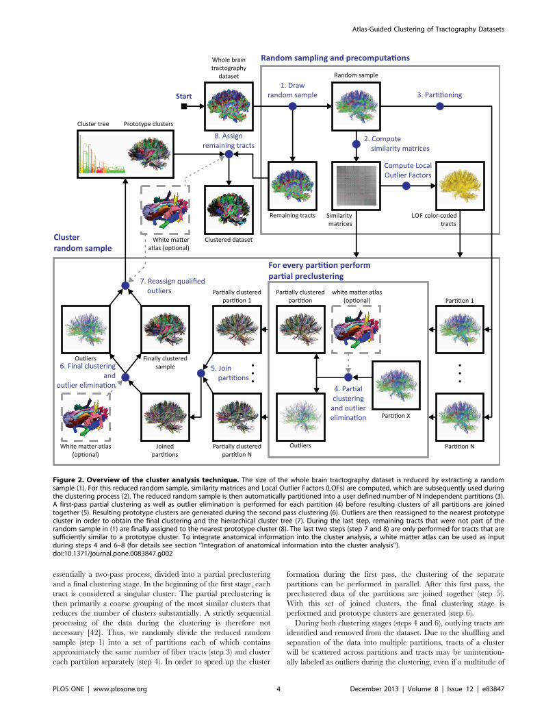
Figure 2. Overview of the cluster analysis technique. The size of the whole brain tractography dataset is reduced by extracting a randomsample (1). For this reduced random sample, similarity matrices and Local Outlier Factors (LOFs) are computed, which are subsequently used duringthe clustering process (2). The reduced random sample is then automatically partitioned into a user defined number of N independent partitions (3).A first-pass partial clustering as well as outlier elimination is performed for each partition (4) before resulting clusters of all partitions are joinedtogether (5). Resulting prototype clusters are generated during the second pass clustering (6). Outliers are then reassigned to the nearest prototypecluster in order to obtain the final clustering and the hierarchical cluster tree (7). During the last step, remaining tracts that were not part of therandom sample in (1) are finally assigned to the nearest prototype cluster (8). The last two steps (step 7 and 8) are only performed for tracts that aresufficiently similar to a prototype cluster. To integrate anatomical information into the cluster analysis, a white matter atlas can be used as inputduring steps 4 and 6–8 (for details see section ‘‘Integration of anatomical information into the cluster analysis’’).doi:10.1371/journal.pone.0083847.g002
Atlas-Guided Clustering of Tractography Datasets
PLOS ONE | www.plosone.org 4 December 2013 | Volume 8 | Issue 12 | e83847
similar tracts are situated nearby but are placed in other partitions.
To warrant that outlying tracts are true outliers, tracts that were
previously labeled as outliers are reevaluated and assigned to the
nearest prototype cluster (step 7) if the similarity between tracts
and cluster is sufficiently high (for details see section ‘‘Assigning
and reassigning tracts’’). In the final step, remaining tracts that are
not part of the reduced random sample (step 1) and have not been
appointed to a cluster yet, are also assigned to the nearest
prototype cluster (step 8) if the similarity between cluster and tracts
is high (for details see section ‘‘Assigning and reassigning tracts’’).
During the whole clustering process, a hierarchical cluster tree
that contains all successive merging steps is generated. The cluster
tree enables not only the visualization of the individual clustering
steps with dendrograms, but also the retrospective extraction of
bundles or a subset of tracts from the bundles.
Formation of clusters. Conceptually, CATSER employs
agglomerative hierarchical clustering during both clustering stages
(steps 4 and 6 in Figure 2). Starting with a set of clusters, the
iterative clustering process is performed until certain stopping
criteria are satisfied (e.g. a user-defined number of clusters is
reached). In each iteration of the clustering, the two most similar
clusters are selected and merged to form a new cluster.
In order to determine the similarity between two clusters, only a
subset of tracts from each cluster is considered. This subset consists
of a set of well distributed tracts that capture the geometry of the
cluster and act as representative tracts. To start the selection of
appropriate representatives tracts, the center of the cluster is
determined by locating the cluster medoid. For a cluster C with
DCD tracts, the medoid mC is defined as the tract in C whose
average distance or dissimilarity to all tracts in C is minimal:
mC~ minp[C
1
DCD
Xq[C
d(p,q)
!: ð4Þ
After the medoid has been identified, representative tracts are
determined iteratively and added to the set of representatives RC .
In every iteration, the tract in C that has the maximum distance to
the medoid mC as well as to all other representatives in RC
becomes a new representative and is added to RC . This iterative
selection process guarantees that the representatives are well
distributed across the cluster. An important aspect for the selection
of representatives is the number of representatives that are used for
the clustering. In practice, this is a trade-off between correct
clustering, accurately assessing the cluster shape, achieving
computational efficiency and robustness to noise. Clusters are
not static, but evolve and grow. Therefore a fixed number of
representatives cannot be used, as all tracts of the cluster would
become a representative if the size of the cluster is smaller than the
number of representatives. By reducing the ratio between number
of representatives DRC D and the cluster size DCD with DRC DvDCD, the
selection algorithm can reject tracts that are outlying. In order to
select DRC D, we briefly divide the cluster formation process into two
stages. In the first stage, we chose DRC D with respect to the
individual size of each cluster and carefully adapt it to reflect
changes in the cluster size. As the cluster size and the number of
representatives increases the computational efficiency decreases
due to the additional calculations that have to be performed for
each additional representative. In order to maintain the compu-
tational efficiency, we define a second stage with a constant
number of representatives. To select the number of representa-
tives, we use a monotonically increasing, piecewise-defined
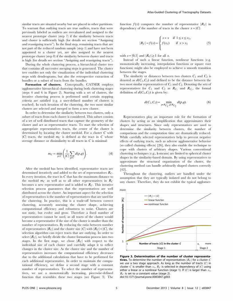
function that resembles these two stages (see Figure 3). The
function f (x) computes the number of representative DRC D in
dependency of the number of tracts in the cluster x~DCD:
jRC j~f (x)~
s|x if 1ƒxƒx1,
f (x1) if xwx1
8><>: ð5Þ
with s~�0,1� and DRC D§1 for all x.
Instead of such a linear function, nonlinear functions (e.g.
monotonically increasing, interpolation functions or square root
functions) might also be employed to achieve a smooth transition
between the stages.
The similarity or distances between two clusters C1 and C2 is
denoted as d(C1,C2) and defined to be the distance between the
two most similar representatives of C1 and C2. Denoting the sets of
representatives for C1 and C2 as RC1and RC2
, the formal
definition of d(C1,C2) is given by:
d(C1,C2)~ minp[RC1
,q[RC2
d(p,q): ð6Þ
Representatives play an important role for the formation of
clusters by acting as an simplification that approximates their
shapes and structures. Since only representatives are used to
determine the similarity between clusters, the number of
comparisons and the computation time are dramatically reduced.
While carefully selected representatives help to prevent negative
effects of outlying tracts, such as adverse agglomerative behavior
(so called chaining effects) [26], they also enable the technique to
cope with clusters of arbitrary shapes. Various conventional
clustering techniques (e.g., k-means) are limited to spherical cluster
shapes in the similarity-based domain. By using representatives to
approximate the structural organization of the cluster, the
clustering method can handle arbitrarily shaped clusters correctly
[42].
Throughout the clustering, outliers are handled under the
assumption that they are typically isolated and do not belong to
any cluster. Therefore, they do not exhibit the typical agglomer-
Figure 3. Determination of the number of cluster representa-tives. To determine the number of representatives DRC D for a cluster Cwe use a two stage approach. As long as the number of tracts DCD incluster C is smaller than x1 , RC is selected in dependency of DCD usingeither a linear or a nonlinear function (stage 1). If DCD is larger than x1 ,RC is set to a constant value (stage 2).doi:10.1371/journal.pone.0083847.g003
Atlas-Guided Clustering of Tractography Datasets
PLOS ONE | www.plosone.org 5 December 2013 | Volume 8 | Issue 12 | e83847
ative behavior in contrast to real clusters [42]. In comparison to
tracts that belong to a cluster, the neighborhoods of outliers are
generally sparse and distances to other tracts of the dataset are
significantly larger. Consequently, clusters that grow very slow and
contain only few tracts at the end of the clustering are labeled as
outliers.
Local Outlier Factor (LOF). Local outlier factors [44] are a
density-based approach to obtain a score for each tract that
specifies its outlierness. By employing the precomputed tract-
similarities, the density distribution of the tracts is analyzed to
compute the LOFs. First, the k-Nearest Neighbors (k-NNs, i.e. the
k-most similar tracts) are determined for each tract. The distances
to these k-NNs are then utilized to compute the local tract density
for each tract. With the local tract density as well as the local tract
density of its k-NNs, the LOF of each tract is calculated.
Practically, a LOF is an estimate on how outlying a tract is
compared to its k-most similar tracts.
LOFs have the favorable property to specify an outlierness-
rating for each tract instead of a fixed labeling that indicates
whether the tract is either an outlier or not. While the LOFs
capture the sparsity of the neighborhood for each tract with a
single value, the upper bound of the LOFs depends on the
similarities in the dataset. Tracts that lie deep inside of a cluster
have a LOF that is approximately 1 or less, whereas the LOF of
tracts increases the more isolated the tracts are. An extensive
discussion about the bounds of LOFs can be found in the original
publication by Breunig et al. [44]. An artificial example of the
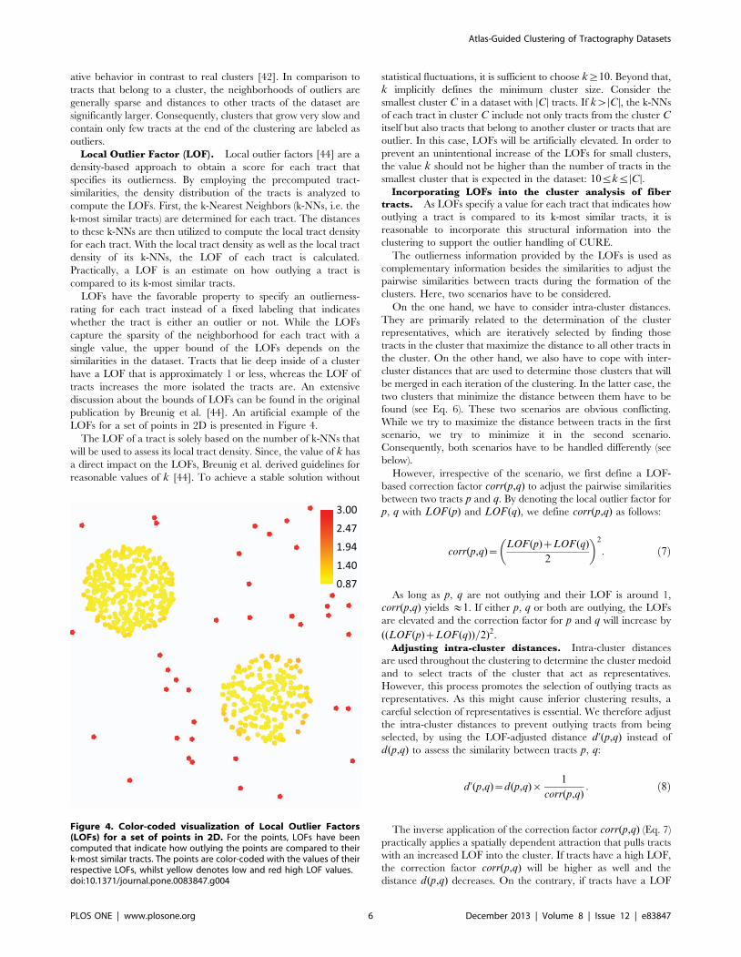
LOFs for a set of points in 2D is presented in Figure 4.
The LOF of a tract is solely based on the number of k-NNs that
will be used to assess its local tract density. Since, the value of k has
a direct impact on the LOFs, Breunig et al. derived guidelines for
reasonable values of k [44]. To achieve a stable solution without
statistical fluctuations, it is sufficient to choose k§10. Beyond that,
k implicitly defines the minimum cluster size. Consider the
smallest cluster C in a dataset with DCD tracts. If kwDCD, the k-NNs
of each tract in cluster C include not only tracts from the cluster Citself but also tracts that belong to another cluster or tracts that are
outlier. In this case, LOFs will be artificially elevated. In order to
prevent an unintentional increase of the LOFs for small clusters,
the value k should not be higher than the number of tracts in the
smallest cluster that is expected in the dataset: 10ƒkƒDCD.Incorporating LOFs into the cluster analysis of fiber
tracts. As LOFs specify a value for each tract that indicates how
outlying a tract is compared to its k-most similar tracts, it is
reasonable to incorporate this structural information into the
clustering to support the outlier handling of CURE.
The outlierness information provided by the LOFs is used as
complementary information besides the similarities to adjust the
pairwise similarities between tracts during the formation of the
clusters. Here, two scenarios have to be considered.
On the one hand, we have to consider intra-cluster distances.
They are primarily related to the determination of the cluster
representatives, which are iteratively selected by finding those
tracts in the cluster that maximize the distance to all other tracts in
the cluster. On the other hand, we also have to cope with inter-
cluster distances that are used to determine those clusters that will
be merged in each iteration of the clustering. In the latter case, the
two clusters that minimize the distance between them have to be
found (see Eq. 6). These two scenarios are obvious conflicting.
While we try to maximize the distance between tracts in the first
scenario, we try to minimize it in the second scenario.
Consequently, both scenarios have to be handled differently (see
below).
However, irrespective of the scenario, we first define a LOF-
based correction factor corr(p,q) to adjust the pairwise similarities
between two tracts p and q. By denoting the local outlier factor for
p, q with LOF (p) and LOF (q), we define corr(p,q) as follows:
corr(p,q)~LOF (p)zLOF (q)
2
� �2
: ð7Þ
As long as p, q are not outlying and their LOF is around 1,
corr(p,q) yields &1. If either p, q or both are outlying, the LOFs
are elevated and the correction factor for p and q will increase by
((LOF (p)zLOF (q))=2)2.
Adjusting intra-cluster distances. Intra-cluster distances
are used throughout the clustering to determine the cluster medoid
and to select tracts of the cluster that act as representatives.
However, this process promotes the selection of outlying tracts as
representatives. As this might cause inferior clustering results, a
careful selection of representatives is essential. We therefore adjust
the intra-cluster distances to prevent outlying tracts from being
selected, by using the LOF-adjusted distance d ’(p,q) instead of
d(p,q) to assess the similarity between tracts p, q:
d ’(p,q)~d(p,q)|1
corr(p,q): ð8Þ
The inverse application of the correction factor corr(p,q) (Eq. 7)
practically applies a spatially dependent attraction that pulls tracts
with an increased LOF into the cluster. If tracts have a high LOF,
the correction factor corr(p,q) will be higher as well and the
distance d(p,q) decreases. On the contrary, if tracts have a LOF
Figure 4. Color-coded visualization of Local Outlier Factors(LOFs) for a set of points in 2D. For the points, LOFs have beencomputed that indicate how outlying the points are compared to theirk-most similar tracts. The points are color-coded with the values of theirrespective LOFs, whilst yellow denotes low and red high LOF values.doi:10.1371/journal.pone.0083847.g004
Atlas-Guided Clustering of Tractography Datasets
PLOS ONE | www.plosone.org 6 December 2013 | Volume 8 | Issue 12 | e83847

that is &1, the tracts are practically not affected. Due to this
reciprocal effect, tracts with a high LOF will suffer a penalty and
have a reduced distance to the medoid and to other representatives
(see Figure 5). This decreases the possibility that outlying tracts
with a high LOF are selected as representatives of a cluster.
Adjusting inter-cluster distances. To adjust the distance
between two different clusters C1 and C2 (see Eq. 6), we weight the
distances d(p,q) between two representative tracts p, q with the
LOF-based correction corr(p,q). This yields the new LOF-
adjusted distance, dcorr, between C1 and C2:
dcorr(C1,C2)~ minp[RC1
,q[RC2
d ’’(p,q), ð9Þ
d ’’(p,q)~d(p,q)|corr(p,q): ð10Þ
This correction affects only the distances between the clusters
and has an influence on when and which clusters are merged. In
order to understand the mechanism behind the correction, the
clustering should be considered as a continuous process in which
clusters are not yet finished but are successively formed. If the
LOF for the representatives of two distinct clusters is &1, the
distance between the clusters is not altered. By definition, these
representatives have to belong to true clusters and are inside the
clusters (otherwise the LOF would not be &1). If representatives
are located at the boundaries of a cluster (compare Figure 4), their
LOF is slightly increased. As a result, the clusters will experience
minimum repulsion and will be clustered slightly later due to their
increased distance. If either one or both representatives of the
clusters are outlier, they will possess a high LOF. As a result of the
LOF-correction, the distance between the clusters will consider-
ably increase and they will be merged substantially later (if they are
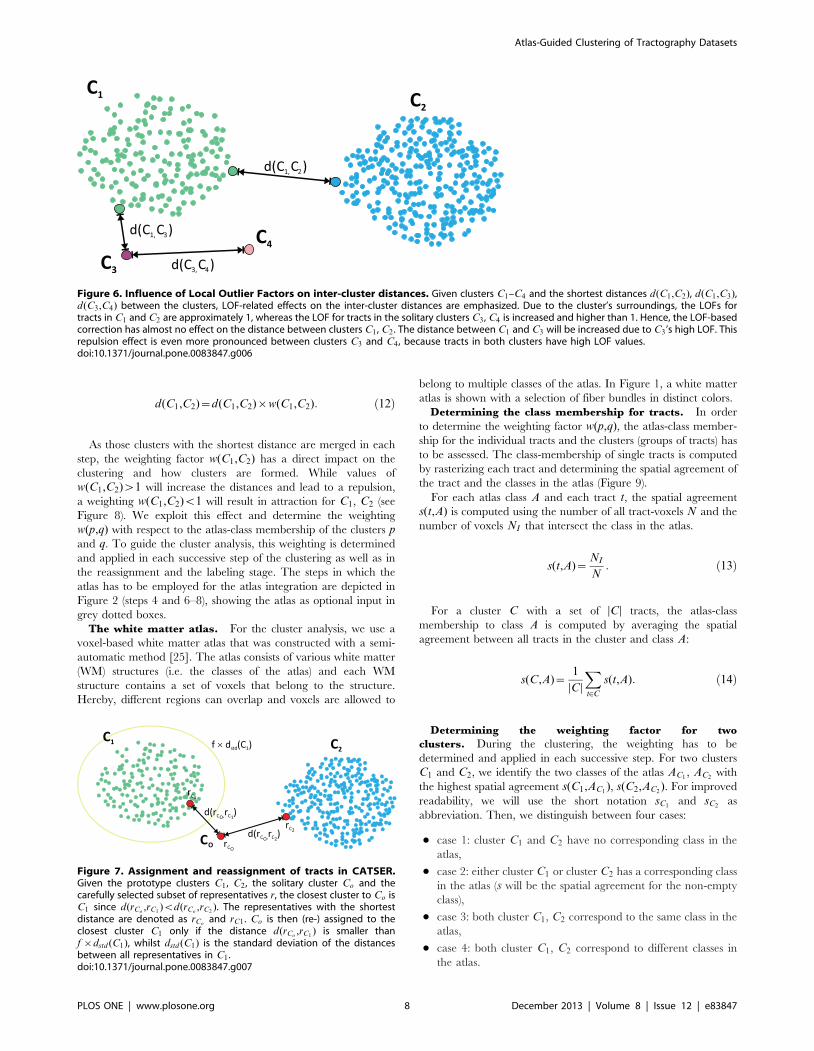
merged at all). An exemplary illustration that depicts the
adjustment of the inter-cluster distances for an artificial set of
points in 2D is given in Figure 6.
This correction effectively contributes to the employed outlier
elimination strategy, which is based on the assumption that
outlying tracts will be far more isolated than other tracts. As a
result of the LOF correction, outlying tracts or clusters will become
even more isolated and will therefore be clustered not at all or in
the very end.
Assigning and reassigning tracts. In CURE and CAT-
SER, slowly growing clusters that contain only few tracts in the
end of the clustering are labeled as outliers. Due to the randomized
division of the data into multiple partitions during the clustering,
tracts may be unintentionally labeled as outliers, even if a
multitude of tracts are spatially located nearby in other partitions.
In order to correct for possibly wrong outlier assignment, outlier
are reevaluated. The distances to all extracted clusters are assessed
and outliers are reassigned to the most similar cluster if the
similarity between outlier and cluster is high enough.
By treating the outlying tract o as a singular cluster Co that
consists only of tract o, the distance d(Co,Cx) to all regular clusters
Cx is computed, with x~1 . . . N and N being the number of
regular clusters. The cluster with the minimum distance to Co is
denoted as CM and the two closest representatives of Co and CM
are termed rCoand rCM
respectively. If dstd (CM ) is the standard
deviation of the distance between all representatives in CM and the
inequality.
d(Co,CM )ƒf |dstd (CM ) ð11Þ
is satisfied, tract o is assigned to CM (see Figure 7). Otherwise o
is labeled as outlier. The factor f can be chosen arbitrarily and is
used to regulate how similar tracts need to be, in order to permit
the reassignment. A value of f ~1 . . . 2 works usually quite well.
Subsequent to the clustering and the reassignment of wrongly
labeled tracts, the set of tracts CE that were not part of the initial
random sample (step 1 in Figure 2) have to be processed. Hereby,
they are either assigned to the nearest cluster or labeled as outlier.
This processing step is carried out in a similar way as the
reassignment above. For each tract o[CE the distance to all
regular clusters is computed and tract o is assigned to the nearest
cluster if inequality 11 is satisfied. As the computation of the LOFs
for the entire dataset is too time consuming (the whole similarity
matrix has to be available), we assume that the LOF of each tract
in CE is 1.
Integration of Anatomical Information into the ClusterAnalysis
In order to incorporate anatomical information into the cluster
analysis, we utilize a white matter atlas that contains various fiber
bundles. As the clustering is based on the principle of merging
clusters with the highest similarity, an effective way to influence
the clustering is to modulate the distance d(C1,C2) between the
clusters C1 and C2:
Figure 5. Influence of Local Outlier Factors on intra-cluster distances. Given one cluster C and the set of tracts fp,q,r,sg[C, the influence ofLOFs on the intra-cluster distances between p and the exemplary tracts q,r,s is unveiled. In the example, the LOF of p, q is approximately one, the LOFof r is slightly increased and the LOF of s is considerably elevated. Since a reciprocal relation is used for the computation of intra-cluster distancescompared to inter-cluster distances, high LOFs result in reduced distances between tracts – an attraction effect. Therefore, the LOF-corrected distancebetween p, s is considerably reduced, while the correction only slightly reduces the distance between p, r. Since p, q are not outlying (LOF &1), theLOF correction has almost no effect on the distance between p, q.doi:10.1371/journal.pone.0083847.g005
Atlas-Guided Clustering of Tractography Datasets
PLOS ONE | www.plosone.org 7 December 2013 | Volume 8 | Issue 12 | e83847
d(C1,C2)~d(C1,C2)|w(C1,C2): ð12Þ
As those clusters with the shortest distance are merged in each
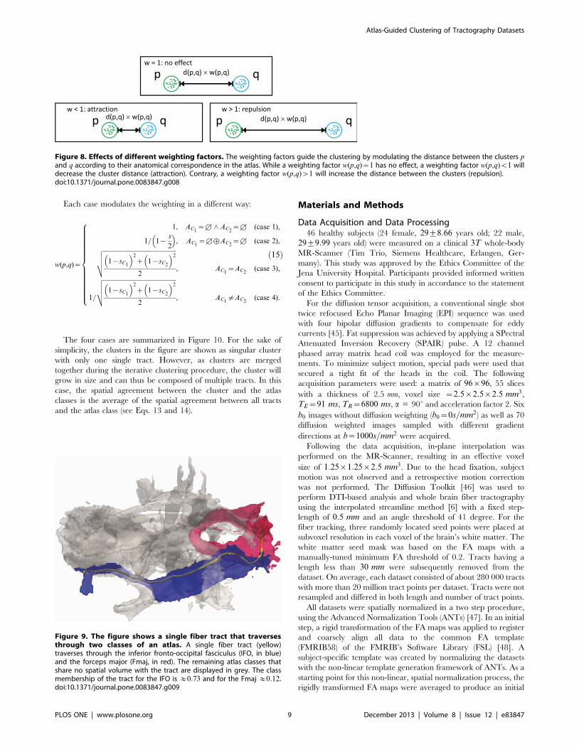
step, the weighting factor w(C1,C2) has a direct impact on the
clustering and how clusters are formed. While values of
w(C1,C2)w1 will increase the distances and lead to a repulsion,
a weighting w(C1,C2)v1 will result in attraction for C1, C2 (see
Figure 8). We exploit this effect and determine the weighting
w(p,q) with respect to the atlas-class membership of the clusters p
and q. To guide the cluster analysis, this weighting is determined
and applied in each successive step of the clustering as well as in
the reassignment and the labeling stage. The steps in which the
atlas has to be employed for the atlas integration are depicted in
Figure 2 (steps 4 and 6–8), showing the atlas as optional input in
grey dotted boxes.
The white matter atlas. For the cluster analysis, we use a
voxel-based white matter atlas that was constructed with a semi-
automatic method [25]. The atlas consists of various white matter
(WM) structures (i.e. the classes of the atlas) and each WM
structure contains a set of voxels that belong to the structure.
Hereby, different regions can overlap and voxels are allowed to
belong to multiple classes of the atlas. In Figure 1, a white matter
atlas is shown with a selection of fiber bundles in distinct colors.
Determining the class membership for tracts. In order
to determine the weighting factor w(p,q), the atlas-class member-
ship for the individual tracts and the clusters (groups of tracts) has
to be assessed. The class-membership of single tracts is computed
by rasterizing each tract and determining the spatial agreement of
the tract and the classes in the atlas (Figure 9).
For each atlas class A and each tract t, the spatial agreement
s(t,A) is computed using the number of all tract-voxels N and the
number of voxels NI that intersect the class in the atlas.
s(t,A)~NI
N: ð13Þ
For a cluster C with a set of DCD tracts, the atlas-class
membership to class A is computed by averaging the spatial
agreement between all tracts in the cluster and class A:
s(C,A)~1
DCD
Xt[C
s(t,A): ð14Þ
Determining the weighting factor for two
clusters. During the clustering, the weighting has to be
determined and applied in each successive step. For two clusters
C1 and C2, we identify the two classes of the atlas AC1, AC2
with
the highest spatial agreement s(C1,AC1), s(C2,AC2
). For improved
readability, we will use the short notation sC1and sC2
as
abbreviation. Then, we distinguish between four cases:
N case 1: cluster C1 and C2 have no corresponding class in the
atlas,
N case 2: either cluster C1 or cluster C2 has a corresponding class
in the atlas (s will be the spatial agreement for the non-empty
class),
N case 3: both cluster C1, C2 correspond to the same class in the
atlas,
N case 4: both cluster C1, C2 correspond to different classes in
the atlas.
Figure 6. Influence of Local Outlier Factors on inter-cluster distances. Given clusters C1–C4 and the shortest distances d(C1,C2), d(C1,C3),d(C3,C4) between the clusters, LOF-related effects on the inter-cluster distances are emphasized. Due to the cluster’s surroundings, the LOFs fortracts in C1 and C2 are approximately 1, whereas the LOF for tracts in the solitary clusters C3 , C4 is increased and higher than 1. Hence, the LOF-basedcorrection has almost no effect on the distance between clusters C1 , C2 . The distance between C1 and C3 will be increased due to C3 ’s high LOF. Thisrepulsion effect is even more pronounced between clusters C3 and C4, because tracts in both clusters have high LOF values.doi:10.1371/journal.pone.0083847.g006
Figure 7. Assignment and reassignment of tracts in CATSER.Given the prototype clusters C1 , C2, the solitary cluster Co and thecarefully selected subset of representatives r, the closest cluster to Co isC1 since d(rCo
,rC1)vd(rCo
,rC2). The representatives with the shortest
distance are denoted as rCoand rC1. Co is then (re-) assigned to the
closest cluster C1 only if the distance d(rCo,rC1
) is smaller thanf |dstd (C1), whilst dstd (C1) is the standard deviation of the distancesbetween all representatives in C1 .doi:10.1371/journal.pone.0083847.g007
Atlas-Guided Clustering of Tractography Datasets
PLOS ONE | www.plosone.org 8 December 2013 | Volume 8 | Issue 12 | e83847
Each case modulates the weighting in a different way:
w(p,q)~
1, AC1~1 ^ AC2
~1 (case 1),
1= 1{s
2
� �, AC1
~1+AC2~1 (case 2),ffiffiffiffiffiffiffiffiffiffiffiffiffiffiffiffiffiffiffiffiffiffiffiffiffiffiffiffiffiffiffiffiffiffiffiffiffiffiffiffiffiffiffiffiffiffiffiffi
1{sC1
� �2
z 1{sC2
� �2
2
vuut, AC1
~AC2(case 3),
1=
ffiffiffiffiffiffiffiffiffiffiffiffiffiffiffiffiffiffiffiffiffiffiffiffiffiffiffiffiffiffiffiffiffiffiffiffiffiffiffiffiffiffiffiffiffiffiffiffi1{sC1
� �2
z 1{sC2
� �2
2
vuut, AC1
=AC2(case 4):
8>>>>>>>>>>>>><>>>>>>>>>>>>>:
ð15Þ
The four cases are summarized in Figure 10. For the sake of
simplicity, the clusters in the figure are shown as singular cluster
with only one single tract. However, as clusters are merged
together during the iterative clustering procedure, the cluster will
grow in size and can thus be composed of multiple tracts. In this
case, the spatial agreement between the cluster and the atlas
classes is the average of the spatial agreement between all tracts
and the atlas class (see Eqs. 13 and 14).
Materials and Methods
Data Acquisition and Data Processing46 healthy subjects (24 female, 29+8:66 years old; 22 male,
29+9:99 years old) were measured on a clinical 3T whole-body
MR-Scanner (Tim Trio, Siemens Healthcare, Erlangen, Ger-
many). This study was approved by the Ethics Committee of the
Jena University Hospital. Participants provided informed written
consent to participate in this study in accordance to the statement
of the Ethics Committee.
For the diffusion tensor acquisition, a conventional single shot
twice refocused Echo Planar Imaging (EPI) sequence was used
with four bipolar diffusion gradients to compensate for eddy
currents [45]. Fat suppression was achieved by applying a SPectral
Attenuated Inversion Recovery (SPAIR) pulse. A 12 channel
phased array matrix head coil was employed for the measure-
ments. To minimize subject motion, special pads were used that
secured a tight fit of the heads in the coil. The following
acquisition parameters were used: a matrix of 96|96, 55 slices
with a thickness of 2.5 mm, voxel size ~2:5|2:5|2:5 mm3,
TE~91 ms, TR~6800 ms, a = 90u and acceleration factor 2. Six
b0 images without diffusion weighting (b0~0s=mm2) as well as 70
diffusion weighted images sampled with different gradient
directions at b~1000s=mm2 were acquired.
Following the data acquisition, in-plane interpolation was
performed on the MR-Scanner, resulting in an effective voxel
size of 1:25|1:25|2:5 mm3. Due to the head fixation, subject
motion was not observed and a retrospective motion correction
was not performed. The Diffusion Toolkit [46] was used to
perform DTI-based analysis and whole brain fiber tractography
using the interpolated streamline method [6] with a fixed step-
length of 0:5 mm and an angle threshold of 41 degree. For the
fiber tracking, three randomly located seed points were placed at
subvoxel resolution in each voxel of the brain’s white matter. The
white matter seed mask was based on the FA maps with a
manually-tuned minimum FA threshold of 0.2. Tracts having a
length less than 30 mm were subsequently removed from the
dataset. On average, each dataset consisted of about 280 000 tracts
with more than 20 million tract points per dataset. Tracts were not
resampled and differed in both length and number of tract points.
All datasets were spatially normalized in a two step procedure,
using the Advanced Normalization Tools (ANTs) [47]. In an initial
step, a rigid transformation of the FA maps was applied to register
and coarsely align all data to the common FA template
(FMRIB58) of the FMRIB’s Software Library (FSL) [48]. A
subject-specific template was created by normalizing the datasets
with the non-linear template generation framework of ANTs. As a
starting point for this non-linear, spatial normalization process, the
rigidly transformed FA maps were averaged to produce an initial
Figure 8. Effects of different weighting factors. The weighting factors guide the clustering by modulating the distance between the clusters pand q according to their anatomical correspondence in the atlas. While a weighting factor w(p,q)~1 has no effect, a weighting factor w(p,q)v1 willdecrease the cluster distance (attraction). Contrary, a weighting factor w(p,q)w1 will increase the distance between the clusters (repulsion).doi:10.1371/journal.pone.0083847.g008
Figure 9. The figure shows a single fiber tract that traversesthrough two classes of an atlas. A single fiber tract (yellow)traverses through the inferior fronto-occipital fasciculus (IFO, in blue)and the forceps major (Fmaj, in red). The remaining atlas classes thatshare no spatial volume with the tract are displayed in grey. The classmembership of the tract for the IFO is &0:73 and for the Fmaj &0:12.doi:10.1371/journal.pone.0083847.g009
Atlas-Guided Clustering of Tractography Datasets
PLOS ONE | www.plosone.org 9 December 2013 | Volume 8 | Issue 12 | e83847

FA template. The template was refined and improved in four
iterations using the greedy SyN transformation model and the
cross correlation metric of ANTs. The resulting transformation
matrices and displacement fields were finally employed to transfer
the fiber tracts into the space of the newly generated template.
White Matter Atlas GenerationWe constructed a white matter atlas with a semi-automatic
method [25]. Out of the 46 spatially normalized datasets (see
previous section), 15 randomly selected datasets were employed to
generate the atlas. We selected 16 WM structures (WM bundles) to
be included in the atlas: forceps major (Fmaj), the frontal
projection of the corpus callosum (the forceps minor – Fmin) as
well as the following bundles of the left and right hemisphere:
anterior thalamic radiation (ATR), gyrus part of the cingulum
cingulate (CGC), hippocampal part of the cingulum (CGH),
cortico-spinal tract (CST), inferior fronto-occipital fasciculus
(IFO), temporal part of the superior longitudinal fasciculus (SLFt),
uncinate fasciculus (UNC). To delineate these bundles, a set of
Regions Of Interests (ROIs) was drawn for each bundle, taking
into account the guidelines for reproducible extraction by Wakana
et al. [24]. For each dataset, tracts that crossed these ROIs were
extracted and assigned to the corresponding WM bundle. While
this is an efficient and fast way to extract the WM fiber bundles, it
only extracts the major parts of the bundles. Tracts that belonged
to the bundle but had not crossed all ROIs were not assigned to
the bundle. This probably resulted in a loss of minuscule details for
the bundles.
The probabilistic white matter atlas was then created by using
the extracted bundles (K~16) of all datasets (N~15). With all
these bundles, the 16 prototype classes of the white matter atlas
were generated. Hereby, each class in the atlas contains all voxels
that are associated with the corresponding atlas class and describes
how reliably each voxel can be associated with this class. Let
A1, . . . ,AK be the prototype classes. If A is one of these classes, it
formally consists of a list of voxels vA~fv1, . . . ,vng with an
unknown number of voxels n that belong to class A. Each vi[vA is
a set of coordinates vi~fx,y,zg that describes the position of voxel
vi in the 3D dataset. The probability that voxel vi belongs to class
A is denoted by wA(vi). As vA consists only of voxels that belong to
A, the probability for each voxel vi[vA is wA(vi)w0. wA(vi) is
therefore bounded by �0,1�.To generate the probabilistic atlas a two step procedure was
used. During the first step, the probabilities for each fiber bundle
were computed individually for each dataset, before these
probabilities were used to generate the final prototype classes in
the second step.
For the first step, the computation of the dataset probability wD
is performed individually for each dataset D[fD1, . . . ,DNg.Initially, for each fiber bundle A of dataset D, the tract density
rA is determined. Hereby each tract that belongs to bundle A is
rasterized to a user-defined 3D grid and all voxels
vA~fv1, . . . ,vng that are occupied by the tracts of A are
identified. The tract density rA(vi) for voxel vi is computed by
counting the number of tracts that occupy voxel vi. To obtain the
dataset probability wDA(vi) for voxel vi of bundle A, the ratio
between the tract density rA(vi) and the number of all tracts that
occupy voxel vi is computed:
wDA(vi)~
rA(vi)PKj~1
rj(vi)
: ð16Þ
If only tracts of A occupy voxel vi, the probability wDA(vi) is 1.
After computing the dataset probability for each dataset and
each fiber bundle the final prototype classes are generated in the
second step. For prototype class A, the prototype probability
wA(vi) in voxel vi is defined as the average of all dataset
probabilities wjA(vi) for A in voxel vi with j~1, . . . ,N:
wA(vi)~1
N
XN
j~1
wjA(vi): ð17Þ
If there is no voxel in a bundle A to which the corresponding
bundles of all N datasets contribute, the maximum bundle
probability max (wA) will be less than 1. To prevent such a
Figure 10. The four cases that determine the weighting factor for the atlas guidance. The figure shows the four cases that determine theweighting factor. In order to present and visualize the four cases, the classes of the atlas that correspond to the left and right cingulum bundle areshown in pink and cyan along with two tracts that represent two clusters (shown in red and blue).doi:10.1371/journal.pone.0083847.g010
Atlas-Guided Clustering of Tractography Datasets
PLOS ONE | www.plosone.org 10 December 2013 | Volume 8 | Issue 12 | e83847
degradation of probabilities, the probabilities in each bundle are
normalized to a maximum probability of 1.
During this prototype generation stage, tracts are rasterized to a
3D grid. As tracts are a set of real-valued points in 3D space, the
atlas can be reconstructed for arbitrary grid resolutions. In this
study we used an atlas with 1 mm3 isotropic resolution. Unreliable
voxels with probability less than 0.3 were removed from the atlas,
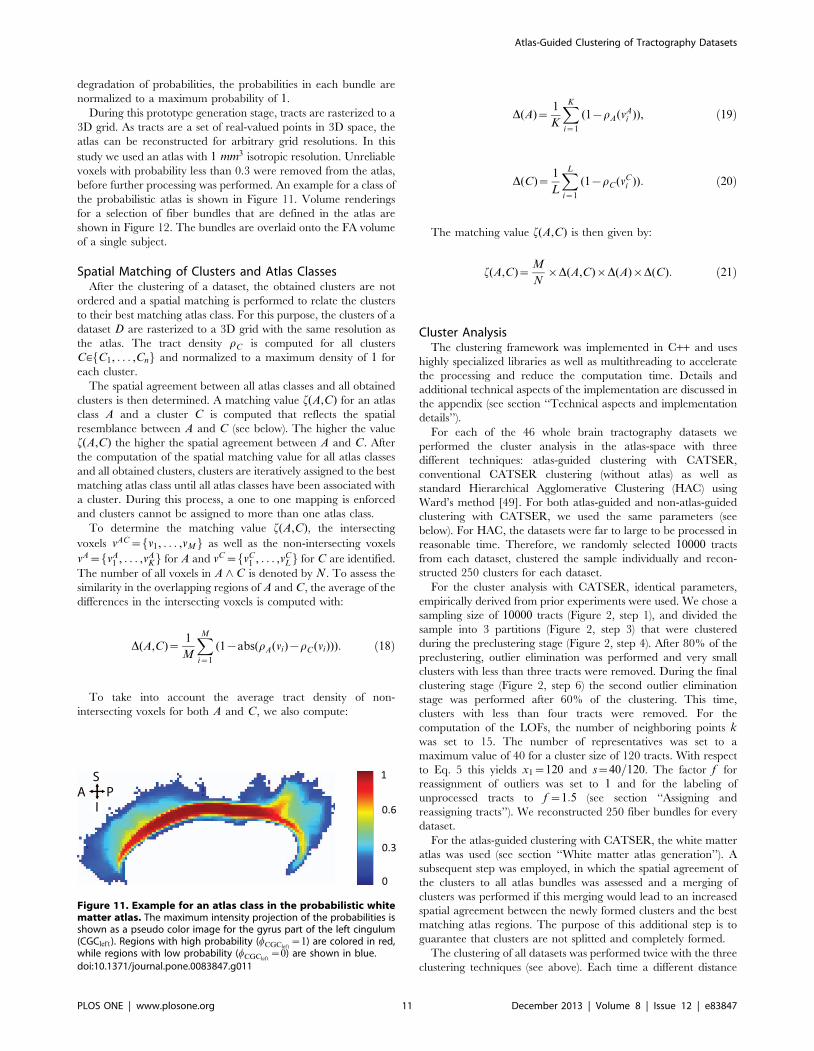
before further processing was performed. An example for a class of
the probabilistic atlas is shown in Figure 11. Volume renderings
for a selection of fiber bundles that are defined in the atlas are
shown in Figure 12. The bundles are overlaid onto the FA volume
of a single subject.
Spatial Matching of Clusters and Atlas ClassesAfter the clustering of a dataset, the obtained clusters are not
ordered and a spatial matching is performed to relate the clusters
to their best matching atlas class. For this purpose, the clusters of a
dataset D are rasterized to a 3D grid with the same resolution as
the atlas. The tract density rC is computed for all clusters
C[fC1, . . . ,Cng and normalized to a maximum density of 1 for
each cluster.
The spatial agreement between all atlas classes and all obtained
clusters is then determined. A matching value f(A,C) for an atlas
class A and a cluster C is computed that reflects the spatial
resemblance between A and C (see below). The higher the value
f(A,C) the higher the spatial agreement between A and C. After
the computation of the spatial matching value for all atlas classes
and all obtained clusters, clusters are iteratively assigned to the best
matching atlas class until all atlas classes have been associated with
a cluster. During this process, a one to one mapping is enforced
and clusters cannot be assigned to more than one atlas class.
To determine the matching value f(A,C), the intersecting
voxels vAC~fv1, . . . ,vMg as well as the non-intersecting voxels
vA~fvA1 , . . . ,vA
Kg for A and vC~fvC1 , . . . ,vC
Lg for C are identified.
The number of all voxels in A ^ C is denoted by N . To assess the
similarity in the overlapping regions of A and C, the average of the
differences in the intersecting voxels is computed with:
D(A,C)~1
M
XMi~1
(1{abs(rA(vi){rC(vi))): ð18Þ
To take into account the average tract density of non-
intersecting voxels for both A and C, we also compute:
D(A)~1
K
XK
i~1
(1{rA(vAi )), ð19Þ
D(C)~1
L
XL
i~1
(1{rC(vCi )): ð20Þ
The matching value f(A,C) is then given by:
f(A,C)~M
N|D(A,C)|D(A)|D(C): ð21Þ
Cluster AnalysisThe clustering framework was implemented in C++ and uses
highly specialized libraries as well as multithreading to accelerate
the processing and reduce the computation time. Details and
additional technical aspects of the implementation are discussed in
the appendix (see section ‘‘Technical aspects and implementation
details’’).
For each of the 46 whole brain tractography datasets we
performed the cluster analysis in the atlas-space with three
different techniques: atlas-guided clustering with CATSER,
conventional CATSER clustering (without atlas) as well as
standard Hierarchical Agglomerative Clustering (HAC) using
Ward’s method [49]. For both atlas-guided and non-atlas-guided
clustering with CATSER, we used the same parameters (see
below). For HAC, the datasets were far to large to be processed in
reasonable time. Therefore, we randomly selected 10000 tracts
from each dataset, clustered the sample individually and recon-
structed 250 clusters for each dataset.
For the cluster analysis with CATSER, identical parameters,
empirically derived from prior experiments were used. We chose a
sampling size of 10000 tracts (Figure 2, step 1), and divided the
sample into 3 partitions (Figure 2, step 3) that were clustered
during the preclustering stage (Figure 2, step 4). After 80% of the
preclustering, outlier elimination was performed and very small
clusters with less than three tracts were removed. During the final
clustering stage (Figure 2, step 6) the second outlier elimination
stage was performed after 60% of the clustering. This time,
clusters with less than four tracts were removed. For the
computation of the LOFs, the number of neighboring points kwas set to 15. The number of representatives was set to a
maximum value of 40 for a cluster size of 120 tracts. With respect
to Eq. 5 this yields x1~120 and s~40=120. The factor f for
reassignment of outliers was set to 1 and for the labeling of
unprocessed tracts to f ~1:5 (see section ‘‘Assigning and
reassigning tracts’’). We reconstructed 250 fiber bundles for every
dataset.
For the atlas-guided clustering with CATSER, the white matter
atlas was used (see section ‘‘White matter atlas generation’’). A
subsequent step was employed, in which the spatial agreement of
the clusters to all atlas bundles was assessed and a merging of
clusters was performed if this merging would lead to an increased
spatial agreement between the newly formed clusters and the best
matching atlas regions. The purpose of this additional step is to
guarantee that clusters are not splitted and completely formed.
The clustering of all datasets was performed twice with the three
clustering techniques (see above). Each time a different distance
Figure 11. Example for an atlas class in the probabilistic whitematter atlas. The maximum intensity projection of the probabilities isshown as a pseudo color image for the gyrus part of the left cingulum(CGCleft). Regions with high probability (wCGCleft
~1) are colored in red,while regions with low probability (wCGCleft
~0) are shown in blue.doi:10.1371/journal.pone.0083847.g011
Atlas-Guided Clustering of Tractography Datasets
PLOS ONE | www.plosone.org 11 December 2013 | Volume 8 | Issue 12 | e83847
measure was used to determine the similarity between the tracts.
We used a Combined Distance (CD) measure [50] as well as the
Hausdorff Distance (HD) (for details about the similarity measures
we refer to section ‘‘Similarity measures’’ in the appendix). In
total, cluster analysis was performed 276 times (46 datasets | 3
clustering techniques | 2 similarity measures).
With spatial matching (see section ‘‘Spatial matching of clusters
and atlas classes’’), clusters were identified and related to their
corresponding and best matching class in the atlas. Inter-
individual matching for bundles of different datasets was not
performed, but can be applied in an additional spatial matching
step, by selecting one dataset to which bundles of remaining
datasets are matched. To evaluate the quality of the final results,
we computed the spatial agreement (see Eq. 13) between the
voxelized clusters and their corresponding, best matching atlas
classes.
To demonstrate the benefits from outlier elimination, the effects
of different outlier elimination strategies and varying levels of noise
were investigated. For this purpose, one dataset that resided in its
native space was segmented according to the guidelines by
Wakana et al. [24]. The same 16 fiber bundles that are also
defined in the atlas (see Figure 12) were extracted. For this
segmented dataset, unsupervised clustering (without white matter
atlas) was performed for varying levels of noise and different sets of
outlier elimination parameters. As the correctness of fiber tract
clusters are visually hard to depict due to their inherent complexity
we used the Euclidean norm between the tract centroids as a
similarity measure for this clustering experiment (see section
‘‘Similarity measures’’ in the appendix). Contrary to fiber tracts,
the distance between the tract centroids can be easily depicted in
3D Euclidean space, which allows good visual delineation of the
clusters and their shapes. For this experiment, the cluster analysis
was performed for three different outlier elimination parameter
sets (low, moderate and high outlier elimination, see Table 1 for
details). In addition, artificial white noise was added to the tract
centroids and gradually increased (0%, 33%, 66%, 99% additional
noise).
Performance AnalysisIn order to assess the performance of the clustering in a
multiprocessing environment, a performance analysis was con-
ducted using a symmetric multiprocessing (SMP) system equipped
with 16 GB main memory and two Intel Xeon processors (L5430,
quad core, 64-bit, 2.66 GHz). Effects on the execution time TP
and the relative speedup SP~T1=TP were investigated by
gradually increasing the number of utilized cores P. T1 is the
execution time if the processing is performed with a single CPU
core. The performance analysis was conducted for the unsuper-
vised clustering without white matter atlas. One dataset D with
100 000 fiber tracts was used, whereas the reduced random sample
consisted of 5000 tracts. The Hausdorff Distance [29] and the
Combined Distance [50] were used as similarity measures. To
impede statistical fluctuations due to running background process,
all computations were repeated ten times.
The analysis of our clustering framework is divided into three
individual parts to identify those parts of the clustering (cmp.
Figure 2) that are suspected to be computationally most critical, as
well as to identify the parts that will profit the most from adding
additional cores:
N Part 1: Computation of the similarity measures for Din
(Figure 2, step 2)
N Part 2: Clustering of the sample dataset Din (Figure 2, steps 3–
7):
The performance during the formation of clusters was
investigated by gradually increasing the number of parallel
clustered partitions.
N Part 3: Labeling of remaining tracts Dout~D\Din (Figure 2,
step 8):
By employing identical clustering parameters as in part 2, the
performance of the labeling was analyzed.
Results
ClusteringThe clustering of all 46 datasets was successfully performed
using the three clustering techniques (atlas-guided CATSER,
CATSER, HAC) and both similarity measures (CD, HD). For
each clustering experiment and each dataset, we matched the
clusters to the atlas classes and determined the best matching
cluster for each class. Clusters for one exemplary dataset,
processed with the atlas-guided CATSER clustering and the
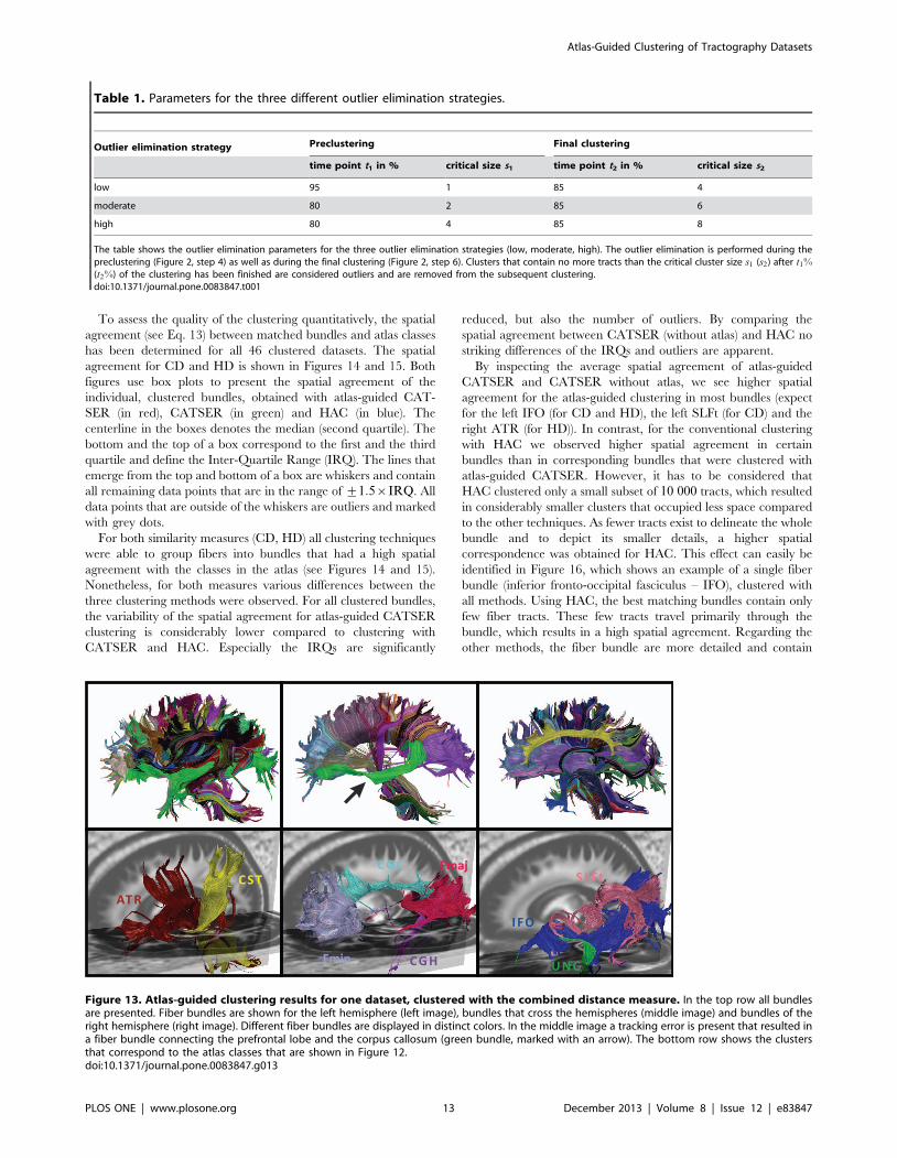
combined distance measure (CD) are shown in Figure 13. All
extracted bundles of the dataset are displayed in the top row. To
enhance the visualization, the bundles in the upper row have been
divided into three groups: bundles of the left hemisphere (left
image), bundles that cross both hemispheres (middle image) and
bundles of the right hemisphere (right image). Fiber bundles are
displayed in distinct colors, and tracts that belong to the same
cluster are colored identically. The matched bundles that
correspond to the atlas classes in Figure 12 are displayed in the
bottom row of Figure 13 with the same coloring as in Figure 12.
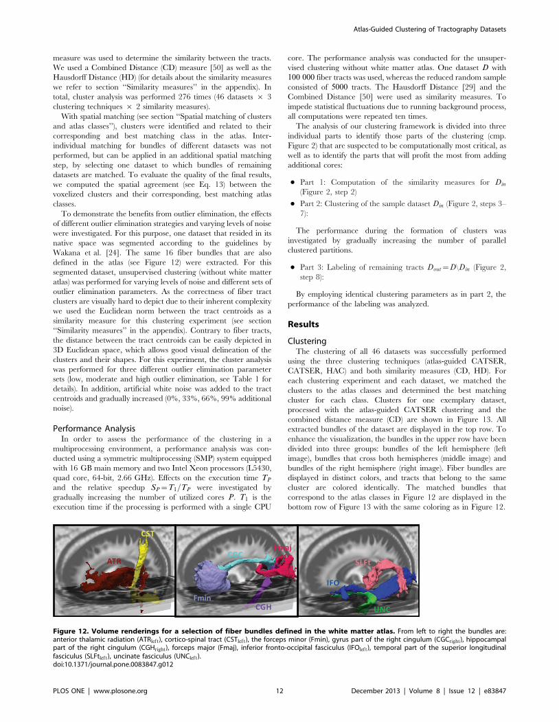
Figure 12. Volume renderings for a selection of fiber bundles defined in the white matter atlas. From left to right the bundles are:anterior thalamic radiation (ATRleft), cortico-spinal tract (CSTleft), the forceps minor (Fmin), gyrus part of the right cingulum (CGCright), hippocampalpart of the right cingulum (CGHright), forceps major (Fmaj), inferior fronto-occipital fasciculus (IFOleft), temporal part of the superior longitudinalfasciculus (SLFtleft), uncinate fasciculus (UNCleft).doi:10.1371/journal.pone.0083847.g012
Atlas-Guided Clustering of Tractography Datasets
PLOS ONE | www.plosone.org 12 December 2013 | Volume 8 | Issue 12 | e83847
To assess the quality of the clustering quantitatively, the spatial
agreement (see Eq. 13) between matched bundles and atlas classes
has been determined for all 46 clustered datasets. The spatial
agreement for CD and HD is shown in Figures 14 and 15. Both
figures use box plots to present the spatial agreement of the
individual, clustered bundles, obtained with atlas-guided CAT-
SER (in red), CATSER (in green) and HAC (in blue). The
centerline in the boxes denotes the median (second quartile). The
bottom and the top of a box correspond to the first and the third
quartile and define the Inter-Quartile Range (IRQ). The lines that
emerge from the top and bottom of a box are whiskers and contain
all remaining data points that are in the range of +1:5|IRQ. All
data points that are outside of the whiskers are outliers and marked
with grey dots.
For both similarity measures (CD, HD) all clustering techniques
were able to group fibers into bundles that had a high spatial
agreement with the classes in the atlas (see Figures 14 and 15).
Nonetheless, for both measures various differences between the
three clustering methods were observed. For all clustered bundles,
the variability of the spatial agreement for atlas-guided CATSER
clustering is considerably lower compared to clustering with
CATSER and HAC. Especially the IRQs are significantly
reduced, but also the number of outliers. By comparing the
spatial agreement between CATSER (without atlas) and HAC no
striking differences of the IRQs and outliers are apparent.
By inspecting the average spatial agreement of atlas-guided
CATSER and CATSER without atlas, we see higher spatial
agreement for the atlas-guided clustering in most bundles (expect
for the left IFO (for CD and HD), the left SLFt (for CD) and the
right ATR (for HD)). In contrast, for the conventional clustering
with HAC we observed higher spatial agreement in certain
bundles than in corresponding bundles that were clustered with
atlas-guided CATSER. However, it has to be considered that
HAC clustered only a small subset of 10 000 tracts, which resulted
in considerably smaller clusters that occupied less space compared
to the other techniques. As fewer tracts exist to delineate the whole
bundle and to depict its smaller details, a higher spatial
correspondence was obtained for HAC. This effect can easily be
identified in Figure 16, which shows an example of a single fiber
bundle (inferior fronto-occipital fasciculus – IFO), clustered with
all methods. Using HAC, the best matching bundles contain only
few fiber tracts. These few tracts travel primarily through the
bundle, which results in a high spatial agreement. Regarding the
other methods, the fiber bundle are more detailed and contain
Table 1. Parameters for the three different outlier elimination strategies.
Outlier elimination strategy Preclustering Final clustering
time point t1 in % critical size s1 time point t2 in % critical size s2
low 95 1 85 4
moderate 80 2 85 6
high 80 4 85 8
The table shows the outlier elimination parameters for the three outlier elimination strategies (low, moderate, high). The outlier elimination is performed during thepreclustering (Figure 2, step 4) as well as during the final clustering (Figure 2, step 6). Clusters that contain no more tracts than the critical cluster size s1 (s2) after t1%
(t2%) of the clustering has been finished are considered outliers and are removed from the subsequent clustering.doi:10.1371/journal.pone.0083847.t001
Figure 13. Atlas-guided clustering results for one dataset, clustered with the combined distance measure. In the top row all bundlesare presented. Fiber bundles are shown for the left hemisphere (left image), bundles that cross the hemispheres (middle image) and bundles of theright hemisphere (right image). Different fiber bundles are displayed in distinct colors. In the middle image a tracking error is present that resulted ina fiber bundle connecting the prefrontal lobe and the corpus callosum (green bundle, marked with an arrow). The bottom row shows the clustersthat correspond to the atlas classes that are shown in Figure 12.doi:10.1371/journal.pone.0083847.g013
Atlas-Guided Clustering of Tractography Datasets
PLOS ONE | www.plosone.org 13 December 2013 | Volume 8 | Issue 12 | e83847
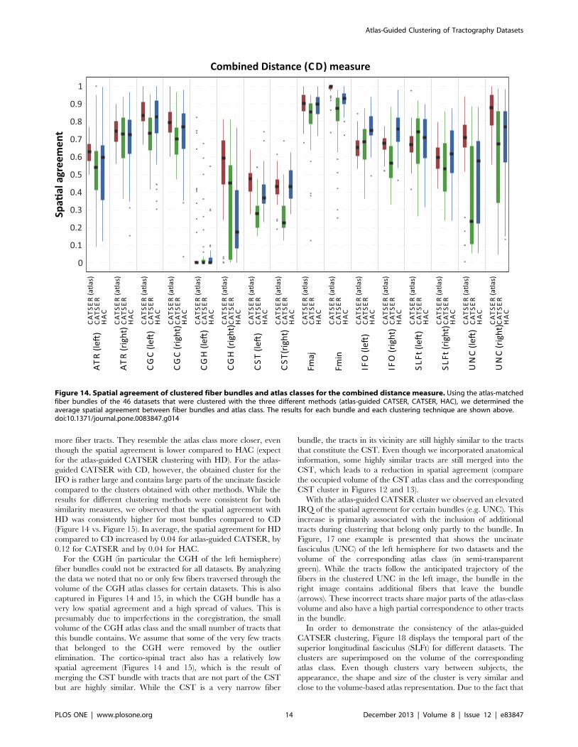
more fiber tracts. They resemble the atlas class more closer, even
though the spatial agreement is lower compared to HAC (expect
for the atlas-guided CATSER clustering with HD). For the atlas-
guided CATSER with CD, however, the obtained cluster for the
IFO is rather large and contains large parts of the uncinate fascicle
compared to the clusters obtained with other methods. While the
results for different clustering methods were consistent for both
similarity measures, we observed that the spatial agreement with
HD was consistently higher for most bundles compared to CD
(Figure 14 vs. Figure 15). In average, the spatial agreement for HD
compared to CD increased by 0.04 for atlas-guided CATSER, by
0.12 for CATSER and by 0.04 for HAC.
For the CGH (in particular the CGH of the left hemisphere)
fiber bundles could not be extracted for all datasets. By analyzing
the data we noted that no or only few fibers traversed through the
volume of the CGH atlas classes for certain datasets. This is also
captured in Figures 14 and 15, in which the CGH bundle has a
very low spatial agreement and a high spread of values. This is
presumably due to imperfections in the coregistration, the small
volume of the CGH atlas class and the small number of tracts that
this bundle contains. We assume that some of the very few tracts
that belonged to the CGH were removed by the outlier
elimination. The cortico-spinal tract also has a relatively low
spatial agreement (Figures 14 and 15), which is the result of
merging the CST bundle with tracts that are not part of the CST
but are highly similar. While the CST is a very narrow fiber
bundle, the tracts in its vicinity are still highly similar to the tracts
that constitute the CST. Even though we incorporated anatomical
information, some highly similar tracts are still merged into the
CST, which leads to a reduction in spatial agreement (compare
the occupied volume of the CST atlas class and the corresponding
CST cluster in Figures 12 and 13).
With the atlas-guided CATSER cluster we observed an elevated
IRQ of the spatial agreement for certain bundles (e.g. UNC). This
increase is primarily associated with the inclusion of additional
tracts during clustering that belong only partly to the bundle. In
Figure, 17 one example is presented that shows the uncinate
fasciculus (UNC) of the left hemisphere for two datasets and the
volume of the corresponding atlas class (in semi-transparent
green). While the tracts follow the anticipated trajectory of the
fibers in the clustered UNC in the left image, the bundle in the
right image contains additional fibers that leave the bundle
(arrows). These incorrect tracts share major parts of the atlas-class
volume and also have a high partial correspondence to other tracts
in the bundle.
In order to demonstrate the consistency of the atlas-guided
CATSER clustering, Figure 18 displays the temporal part of the
superior longitudinal fasciculus (SLFt) for different datasets. The
clusters are superimposed on the volume of the corresponding
atlas class. Even though clusters vary between subjects, the
appearance, the shape and size of the cluster is very similar and
close to the volume-based atlas representation. Due to the fact that
Figure 14. Spatial agreement of clustered fiber bundles and atlas classes for the combined distance measure. Using the atlas-matchedfiber bundles of the 46 datasets that were clustered with the three different methods (atlas-guided CATSER, CATSER, HAC), we determined theaverage spatial agreement between fiber bundles and atlas class. The results for each bundle and each clustering technique are shown above.doi:10.1371/journal.pone.0083847.g014
Atlas-Guided Clustering of Tractography Datasets
PLOS ONE | www.plosone.org 14 December 2013 | Volume 8 | Issue 12 | e83847
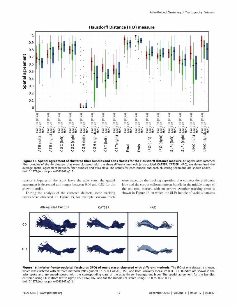
various sub-parts of the SLFt leave the atlas class, the spatial
agreement is decreased and ranges between 0.60 and 0.82 for the
shown bundles.
During the analysis of the clustered datasets, some tracking
errors were observed. In Figure 13, for example, various tracts
were traced by the tracking algorithm that connect the prefrontal
lobe and the corpus callosum (green bundle in the middle image of
the top row, marked with an arrow). Another tracking error is
shown in Figure 18, in which the SLFt bundle of various datasets
Figure 15. Spatial agreement of clustered fiber bundles and atlas classes for the Hausdorff distance measure. Using the atlas-matchedfiber bundles of the 46 datasets that were clustered with the three different methods (atlas-guided CATSER, CATSER, HAC), we determined theaverage spatial agreement between fiber bundles and atlas class. The results for each bundle and each clustering technique are shown above.doi:10.1371/journal.pone.0083847.g015
Figure 16. Inferior fronto-occipital fasciculus (IFO) of one dataset clustered with different methods. The IFO of one dataset is shown,which was clustered with all three methods (atlas-guided CATSER, CATSER, HAC) and both similarity measures (CD, HD). Bundles are shown in theatlas space and are superimposed with the corresponding class of the atlas (in semi-transparent blue). The spatial agreement for the bundlesclustered using CD is (from left to right): 0.58; 0.62; 0.69 and for the bundles clustered using HD: 0.75; 0.67; 0.73.doi:10.1371/journal.pone.0083847.g016
Atlas-Guided Clustering of Tractography Datasets
PLOS ONE | www.plosone.org 15 December 2013 | Volume 8 | Issue 12 | e83847
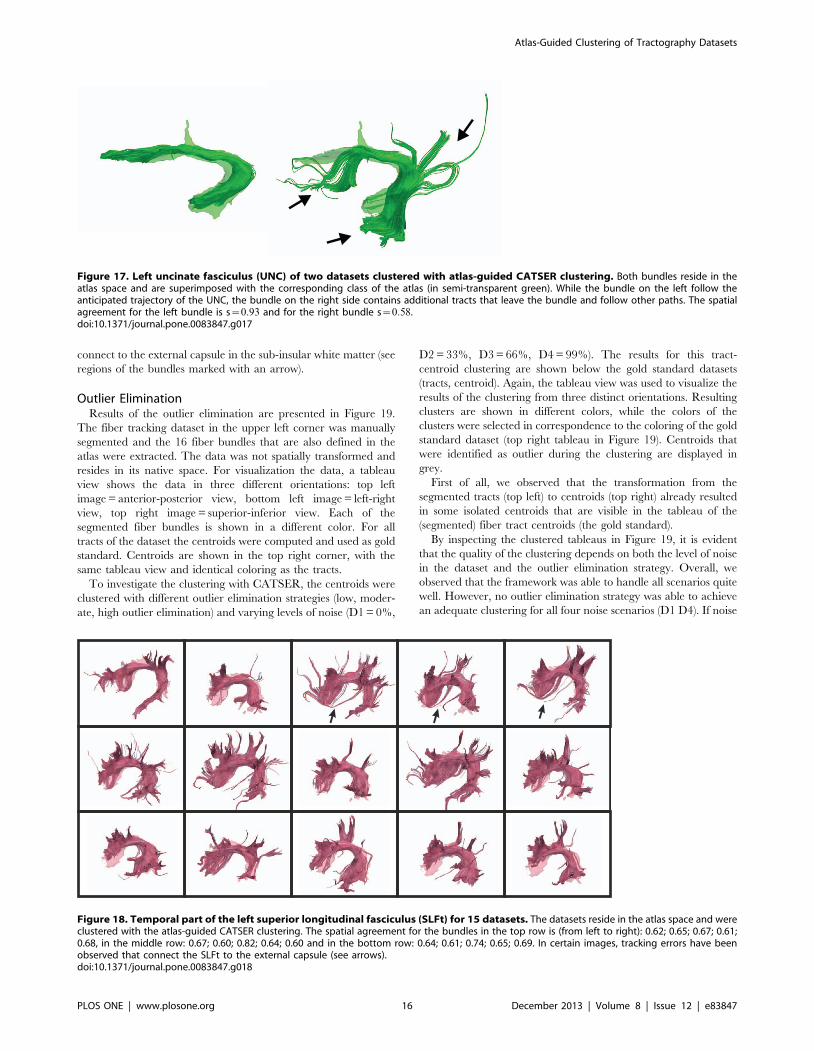
connect to the external capsule in the sub-insular white matter (see
regions of the bundles marked with an arrow).
Outlier EliminationResults of the outlier elimination are presented in Figure 19.
The fiber tracking dataset in the upper left corner was manually
segmented and the 16 fiber bundles that are also defined in the
atlas were extracted. The data was not spatially transformed and
resides in its native space. For visualization the data, a tableau
view shows the data in three different orientations: top left
image = anterior-posterior view, bottom left image = left-right
view, top right image = superior-inferior view. Each of the
segmented fiber bundles is shown in a different color. For all
tracts of the dataset the centroids were computed and used as gold
standard. Centroids are shown in the top right corner, with the
same tableau view and identical coloring as the tracts.
To investigate the clustering with CATSER, the centroids were
clustered with different outlier elimination strategies (low, moder-
ate, high outlier elimination) and varying levels of noise (D1 = 0%,
D2 = 33%, D3 = 66%, D4 = 99%). The results for this tract-
centroid clustering are shown below the gold standard datasets
(tracts, centroid). Again, the tableau view was used to visualize the
results of the clustering from three distinct orientations. Resulting
clusters are shown in different colors, while the colors of the
clusters were selected in correspondence to the coloring of the gold
standard dataset (top right tableau in Figure 19). Centroids that
were identified as outlier during the clustering are displayed in
grey.
First of all, we observed that the transformation from the
segmented tracts (top left) to centroids (top right) already resulted
in some isolated centroids that are visible in the tableau of the
(segmented) fiber tract centroids (the gold standard).
By inspecting the clustered tableaus in Figure 19, it is evident
that the quality of the clustering depends on both the level of noise
in the dataset and the outlier elimination strategy. Overall, we
observed that the framework was able to handle all scenarios quite
well. However, no outlier elimination strategy was able to achieve
an adequate clustering for all four noise scenarios (D1 D4). If noise
Figure 17. Left uncinate fasciculus (UNC) of two datasets clustered with atlas-guided CATSER clustering. Both bundles reside in theatlas space and are superimposed with the corresponding class of the atlas (in semi-transparent green). While the bundle on the left follow theanticipated trajectory of the UNC, the bundle on the right side contains additional tracts that leave the bundle and follow other paths. The spatialagreement for the left bundle is s~0:93 and for the right bundle s~0:58.doi:10.1371/journal.pone.0083847.g017
Figure 18. Temporal part of the left superior longitudinal fasciculus (SLFt) for 15 datasets. The datasets reside in the atlas space and wereclustered with the atlas-guided CATSER clustering. The spatial agreement for the bundles in the top row is (from left to right): 0.62; 0.65; 0.67; 0.61;0.68, in the middle row: 0.67; 0.60; 0.82; 0.64; 0.60 and in the bottom row: 0.64; 0.61; 0.74; 0.65; 0.69. In certain images, tracking errors have beenobserved that connect the SLFt to the external capsule (see arrows).doi:10.1371/journal.pone.0083847.g018
Atlas-Guided Clustering of Tractography Datasets
PLOS ONE | www.plosone.org 16 December 2013 | Volume 8 | Issue 12 | e83847
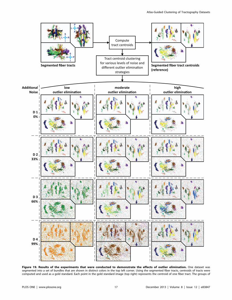
Figure 19. Results of the experiments that were conducted to demonstrate the effects of outlier elimination. One dataset wassegmented into a set of bundles that are shown in distinct colors in the top left corner. Using the segmented fiber tracts, centroids of tracts werecomputed and used as a gold standard. Each point in the gold standard image (top right) represents the centroid of one fiber tract. The groups of
Atlas-Guided Clustering of Tractography Datasets
PLOS ONE | www.plosone.org 17 December 2013 | Volume 8 | Issue 12 | e83847

is barely present (D1, D2), minimal outlier elimination is sufficient
to obtain a good discrimination between the clusters, while a more
aggressive outlier elimination strategy is indispensable if too much
noise is present (D3, D4). If more aggressive outlier elimination
strategies are used for datasets with little noise (e.g. D1, D2), the
outlier elimination rate might be too high and small clusters might
be labeled as outliers. In the opposite case, when plenty of noise is
present (e.g. D3, D4) and minimal outlier elimination is used,
clustering will probably fail and lead to erroneous clusters. In
general, the number of points that were identified as outliers
increases with intensified outlier elimination. Hence we believe
that a moderate outlier elimination strategy seems to be a good
compromise.
However, an increase in noise always has harmful effects on
clustering and will result in degraded performance due to noise
contaminations of the true clusters. The clustering methods will
have difficulties to identify the correct clusters and chaining effects
will lead to merging of distinct clusters. The more noise the more
aggressive the outlier elimination should be in order to achieve
satisfying clustering with good delineation of fiber bundles.
Performance AnalysisThe performance analysis of our clustering framework was
conducted as described in the Materials and methods section.
Figure 20 shows the results of the analysis for the individual parts
of the cluster analysis and the two analyzed similarity measures
(CD, HD). The overall computation time in dependency of the
number of employed CPU cores is shown with a stack plot in the
top row, along with the corresponding speedup in the bottom row.
Due to the separation of the similarity measures from the
clustering, precomputation of the similarity measures (part 1, step
2 in Figure 2) and assignment of remaining tracts to the prototype
clusters (part 3, step 8 in Figure 2) were the most time consuming
parts that accounted for major portions of the computation time.
The actual clustering process that is responsible for the generation
of prototype clusters from the sample (part 2, steps 3–7 in Figure 2)
accounted only for a fraction of the total computation time.
Increasing the number of active CPU cores led to a significant
reduction of the computation time for both distance measures. For
part 1 and part 3, the speedup is nearly linear for CD
(Figures 20C), whereas the speedup is fully sustained for HD as
the number of employed cores increases from 1 to 8 (Figure 20D).
This implies that the HD could be parallelized very efficiently,
whereas the additional CPU cores are not as efficiently used with
CD. However, cluster analysis with CD is still an order of
magnitude faster compared to cluster analysis with HD
(Figure 20A and B).
While the performance analysis was only performed for
unsupervised clustering, we observed an increase in computation
time of approximately 10% for atlas-guided clustering.
Discussion and Conclusion
Due to the high computational complexity of many conven-
tional clustering algorithms, cluster analysis is in practice restricted
to small datasets (e.g. [27,29,33]). In this contribution, we have
introduced a new framework for cluster analysis of tractography
datasets derived from diffusion-weighted MRI data. To assess the
similarity of fiber tracts, the framework contains several proximity
measures that can either be used independently or in conjunction
with other similarity measures to perform clustering in higher
dimensions. Together with practical concepts for cluster analysis of
large tractography datasets, the new clustering method CATSER
has been presented. CATSER exploits the inherent redundancy of
large datasets and separates fiber tracts into meaningful bundles in
reasonable time. Structural information of a white matter atlas can
be incorporated into the clustering to achieve an anatomically
correct and reproducible grouping of fiber tracts. This approach
combines the benefits of classification and clustering and can be
considered a hybrid technique. In addition to the clusters that
correspond to the classes of the atlas, CATSER also extracts
additional clusters that are concealed within the dataset. If an atlas
is not available (e.g., in pediatric cases [51]), the technique can still
be used to cluster large datasets without anatomical guidance. 46
tractography datasets of healthy volunteers have been processed
and clustered with three different clustering techniques and two
similarity measures (Combined Distance (CD) and Hausdorff
Distance (HD)). The presented clustering technique CATSER
(with and without atlas-guidance) and conventional Hierarchical
Agglomerative Clustering (HAC) was used for clustering. With
HAC only a small subset of 10000 tracts was clustered due to the
high computational complexity of HAC.
For the majority of the fiber bundles that corresponded to
classes in the atlas, consistent results were obtained. In order to
quantify the quality of the clustering the spatial agreement
between clustered fiber bundles and their corresponding atlas
classes was assessed. For both similarity measures we observed that
the incorporation of the volumetric atlas clearly resulted in an
improved, more consistent and reproducible clustering of fiber
tracts. While spatial resemblance to the atlas classes increased,
variability decreased. In contrast, both other methods (CATSER
without atlas and HAC) had significantly higher spread of values
for spatial agreement.
The comparison of the utilized similarity measures revealed that
spatial agreement was consistently higher for HD compared to
CD. Even though we expected that incorporating shape similarity
would improve clustering and increase spatial agreement between
clusters and atlas classes, this assumption was not confirmed. One
reason for the lower spatial agreement may be related to the shape
similarity which is an essential part of the CD. The shape similarity
is not computed for the entire tracts but only for matched partial
tract parts to determine the similarity of complete and incomplete
tracts (see section ‘‘Similarity measures’’). If the shape of the
matched tract parts is highly similar, agreement rates are also high
even if the tracts are not incomplete but belong to another fiber
bundle. Figure 16 contains an example where the IFO contains a
substantial part that belongs to the UNC. Nevertheless, one has
not only to consider spatial agreement but also computation time.
Here, the cluster analysis with CD was 10 times faster compared to
the cluster analysis with HD.
The spatial correspondence between obtained clusters and atlas
classes was computed by using the number of all cluster voxels and
the number of cluster voxels that intersect the atlas class (see Eq.
13). While this takes into account voxels that are occupied by both
centroids (gold standard) are show in the same color as their corresponding fiber bundles. All data is presented in a tableau view that shows the datain three different orientations: top left image = anterior-posterior view, bottom left image = left-right view, top right image = superior-inferior view.The centroids of the gold standard dataset were clustered using the tract centroid distance as similarity measure. Varying levels of artificial noise (0%,33%, 66% and 99% additional noise) were used and different outlier elimination strategies were tested. The results for the clustering are displayed inthe 4|3 table (D1–D4).doi:10.1371/journal.pone.0083847.g019
Atlas-Guided Clustering of Tractography Datasets
PLOS ONE | www.plosone.org 18 December 2013 | Volume 8 | Issue 12 | e83847
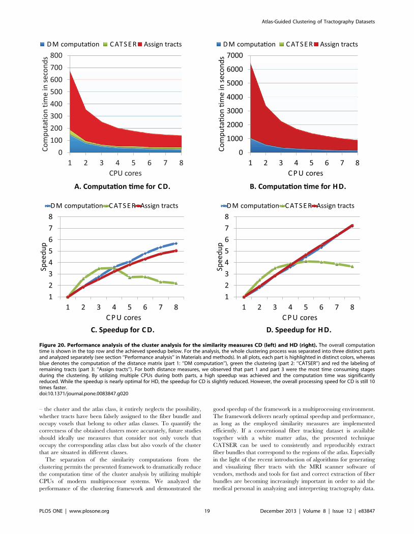
– the cluster and the atlas class, it entirely neglects the possibility,
whether tracts have been falsely assigned to the fiber bundle and
occupy voxels that belong to other atlas classes. To quantify the
correctness of the obtained clusters more accurately, future studies
should ideally use measures that consider not only voxels that
occupy the corresponding atlas class but also voxels of the cluster
that are situated in different classes.
The separation of the similarity computations from the
clustering permits the presented framework to dramatically reduce
the computation time of the cluster analysis by utilizing multiple
CPUs of modern multiprocessor systems. We analyzed the
performance of the clustering framework and demonstrated the
good speedup of the framework in a multiprocessing environment.
The framework delivers nearly optimal speedup and performance,
as long as the employed similarity measures are implemented
efficiently. If a conventional fiber tracking dataset is available
together with a white matter atlas, the presented technique
CATSER can be used to consistently and reproducibly extract
fiber bundles that correspond to the regions of the atlas. Especially
in the light of the recent introduction of algorithms for generating
and visualizing fiber tracts with the MRI scanner software of
vendors, methods and tools for fast and correct extraction of fiber
bundles are becoming increasingly important in order to aid the
medical personal in analyzing and interpreting tractography data.
12345678
1 2 3 4 5 6 7 8
Spee
dup
C P U coresC. Speedup for C D.
A. Computa on me for CD.� �
D. Speedup for H D.
B. Computa on me for HD.� �
D M computa on� C AT S E R Assign tracts
0
1000
2000
3000
4000
5000
6000
7000
1 2 3 4 5 6 7 8
Com
puta
onm
e in
seco
nds
��
C P U cores
D M computa on� C AT S E R Assign tractsD M computa on� C AT S E R Assign tracts
12345678
1 2 3 4 5 6 7 8
Spee
dup
C P U cores
D M computa on� C AT S E R Assign tracts
Figure 20. Performance analysis of the cluster analysis for the similarity measures CD (left) and HD (right). The overall computationtime is shown in the top row and the achieved speedup below. For the analysis, the whole clustering process was separated into three distinct partsand analyzed separately (see section ‘‘Performance analysis’’ in Materials and methods). In all plots, each part is highlighted in distinct colors, whereasblue denotes the computation of the distance matrix (part 1: ‘‘DM computation’’), green the clustering (part 2: ‘‘CATSER’’) and red the labeling ofremaining tracts (part 3: ‘‘Assign tracts’’). For both distance measures, we observed that part 1 and part 3 were the most time consuming stagesduring the clustering. By utilizing multiple CPUs during both parts, a high speedup was achieved and the computation time was significantlyreduced. While the speedup is nearly optimal for HD, the speedup for CD is slightly reduced. However, the overall processing speed for CD is still 10times faster.doi:10.1371/journal.pone.0083847.g020
Atlas-Guided Clustering of Tractography Datasets
PLOS ONE | www.plosone.org 19 December 2013 | Volume 8 | Issue 12 | e83847

Besides the application of CATSER for clustering such single
subject datasets in clinical routine, we believe that the presented
techniques and algorithms are especially useful and important for
the fast and fully automated clustering of multiple datasets that are
supposed to be analyzed with fiber bundle driven techniques for
quantitative analyses.
As an anatomically correct and consistent grouping of tracts for
multiple subjects is difficult to achieve without additional
anatomical information, our technique can incorporate an atlas
to guide the clustering process. We demonstrated that CATSER is
capable to extract bundles that are defined in the atlas and that it
also extracts additional reasonable clusters with conventional
clustering. To influence the cluster generation we computed the
spatial correspondence between tracts and atlas classes and
incorporated this information into the clustering. As the atlas
contains not only the occupied voxels for each atlas class but also
additional probabilistic information, it might be reasonable to
incorporate this information in the future. The atlas contains only
the major parts of the bundles due to the employed ROI-based
extraction technique. Even though the spatial agreement between
obtained clusters and atlas classes was already quite high, we
anticipate that the manual generation of an atlas that captures
even smallest details will increase the spatial agreement between
the clusters and the atlas bundles even further.
The validity and anatomical correctness of the obtained clusters
is not only affected by the cluster analysis algorithm. Both data
quality and preprocessing techniques play a crucial role and
influence the generation of the white matter atlas and the cluster
analysis. In this study, we only used Diffusion Tensor Imaging
(DTI) and deterministic tractography as such techniques are
widely available and often used in clinical routine [51]. However,
the measured diffusion signal is just an approximation of the
underlying microstructure that consists of billions of axonal
connections per imaging voxel [52]. Even though the diffusion
tensor is a good approximation if tissues are homogeneous and
axons are aligned parallel, it is insufficient in heterogeneous tissue,
where multiple fiber compartments give rise to a complex diffusion
signal (e.g. crossing, fanning or kissing fibers). As the tensor
degrades, DTI is incapable to describe the microstructure
properly. In such cases, tractography often fails to reconstruct
meaningful fiber tracts. Tracts may be incorrect, will be disrupted
along the course of the structure or even perform an unreliable
trajectory that follows distinct anatomical structures nearby.
Examples for tracking artifacts and tracts that connect wrong
regions are seen in Figures 13 and 18. A cluster that consisted of
additional spurious tracts is shown in Figure 17. While the
clustering technique can counter some of these imperfections by
using outlier elimination, it will be unable to identify incorrect
tracts if a sufficiently large number of similar misguided tracts
exist. If tracts share major parts of the atlas-class volume and also
have a high (partial) correspondence to the other tracts in the
bundle, the atlas-guided clustering is limited in excluding incorrect
fibers. In order to describe the diffusion in the presence of complex
fiber architectures accurately more elaborate methods have to be
used. With complex techniques that sample the diffusion signal in
many directions with high b-values (e.g. high angular diffusion
imaging [53,54]), Orientation Distribution Functions (ODFs) can
be reconstructed that characterize the diffusion signal more
accurately and are able to resolve regions with crossing fibers.
By employing high angular resolution diffusion imaging in
conjunction with ODF-based tractography techniques [55], we
anticipate significant improvements in the quality of the tracto-
graphy datasets and a reduction of unreasonable clusters. As the
white matter atlas is generated on the basis of reconstructed fiber
tracts, erroneous tractography influences the atlas generation as
well. The connection between the uncinate fasciculus and the
inferior frontal gyrus (see Figure 17) is, for example, missing from
the atlas. Considering heterogeneous tissue where multiple fiber
compartments exist (e.g. crossing fibers), a voxel-based probabi-
listic atlas is limited as probabilities will be significantly reduced in
regions with crossing fibers. An orientation dependent atlas that
takes into account the fiber orientation in each voxel by using, for
example, ODFs, will be the next reasonable step to further
enhance the clustering and to prevent the bundling of misguided
tracts. In addition, a grey matter atlas might also be employed to
improve the clustering. In this case, a weighting factor might be
based on the distance between the tracts and their closest grey
matter region.
Our atlas-guided clustering approach aims at a fast and
consistent extraction of fiber bundles for multiple subjects by
using a white matter atlas. Compared to recent techniques that
have been presented (e.g. [35,39,40]), it enables the anatomically
correct extraction of bundles that are defined in the atlas, as well as
the extraction of additional bundles that are not available in the
atlas. While Guevara et al. [40] uses a reasonably fast approach
that is based on the clustering of voxels, Visser’s algorithm employs
partitioning and repeated hierarchical clustering to achieve a
grouping of tracts. Even though Visser’s technique [39] works
quite well for the clustering of fiber tracts, it is limited by the long
computation times, which make it impractical to cluster large
numbers of datasets. However, while such similarity-based
approaches can be used for grouping fiber tracts, a good
correspondence of the clustered bundles to the true anatomical
bundles cannot be guaranteed due to the lack of anatomical
knowledge. As a result, Guevara et al. extended their voxel
clustering approach to increase anatomical correspondence by
incorporating a white matter atlas [56]. First, agglomerative voxel
clustering is performed until many thousands of clusters remain.
This multitude of clusters is then classified using a manually
labeled white matter atlas, derived from a set of clustered datasets.
A different approach for the anatomically correct extraction of
white matter fiber bundles was proposed by Yendiki et al. [57]
with the TRACULA framework. Instead of using cluster analysis
to retrospectively bundle fiber tracts from whole brain tracto-
graphy datasets, TRACULA aims at the separated reconstruction
of the bundles during the fiber tracking itself. Hereby, probabilistic
tractography is used to reconstruct only the tracts of interest by
restricting the tracking using anatomically a-priori-defined regions
of interest as defined by Wakana et al. [24].
Cluster analysis of fiber tracts is not only based on the clustering
algorithm itself, but fundamentally depends on the employed
similarity measures that define the criteria to distinguish fiber
tracts. Popular measures such as the Hausdorff distance [29], the
Chamfer distance [58] or shape-based similarity measures [59] are
often used to assess the similarity of entire tracts, but neglect
partially overlapping [60] or incomplete fibers. To take into
account partially overlapping fiber tracts, Wassermann et al. [60]
proposed a mathematical framework that modeled tracts and fiber
bundles as Gaussian processes using blurred indicator functions in
voxel space. While the Combined Distance measure (CD) also
takes into account incomplete or partially overlapping fibers,
Wasserman’s similarity measure has also some resemblance to our
atlas-guided clustering. In their framework tracts are successively
formed and the Gaussian processes of the tracts are merged in
each iteration. As this approach is partly similar to our atlas-
guidance, both methods might by suitable to complement each
other.
Atlas-Guided Clustering of Tractography Datasets
PLOS ONE | www.plosone.org 20 December 2013 | Volume 8 | Issue 12 | e83847
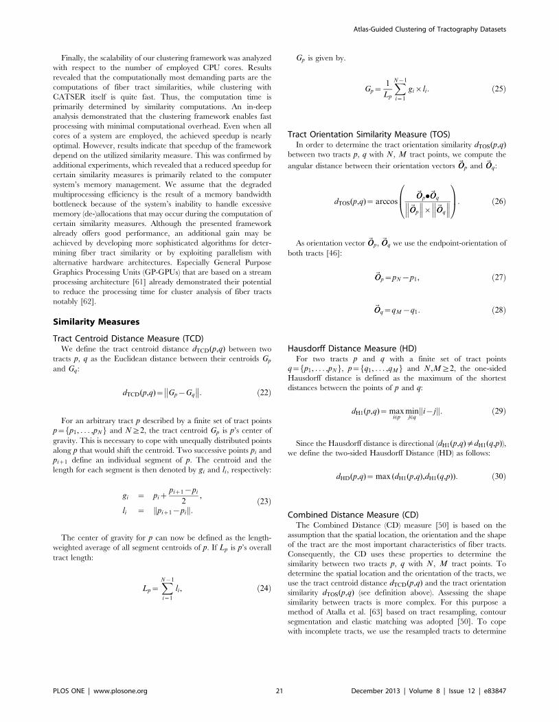
Finally, the scalability of our clustering framework was analyzed
with respect to the number of employed CPU cores. Results
revealed that the computationally most demanding parts are the
computations of fiber tract similarities, while clustering with
CATSER itself is quite fast. Thus, the computation time is
primarily determined by similarity computations. An in-deep
analysis demonstrated that the clustering framework enables fast
processing with minimal computational overhead. Even when all
cores of a system are employed, the achieved speedup is nearly
optimal. However, results indicate that speedup of the framework
depend on the utilized similarity measure. This was confirmed by
additional experiments, which revealed that a reduced speedup for
certain similarity measures is primarily related to the computer
system’s memory management. We assume that the degraded
multiprocessing efficiency is the result of a memory bandwidth
bottleneck because of the system’s inability to handle excessive
memory (de-)allocations that may occur during the computation of
certain similarity measures. Although the presented framework
already offers good performance, an additional gain may be
achieved by developing more sophisticated algorithms for deter-
mining fiber tract similarity or by exploiting parallelism with
alternative hardware architectures. Especially General Purpose
Graphics Processing Units (GP-GPUs) that are based on a stream
processing architecture [61] already demonstrated their potential
to reduce the processing time for cluster analysis of fiber tracts
notably [62].
Similarity Measures
Tract Centroid Distance Measure (TCD)We define the tract centroid distance dTCD(p,q) between two
tracts p, q as the Euclidean distance between their centroids Gp
and Gq:
dTCD(p,q)~ Gp{Gq
�� ��: ð22Þ
For an arbitrary tract p described by a finite set of tract points
p~fp1, . . . ,pNg and N§2, the tract centroid Gp is p’s center of
gravity. This is necessary to cope with unequally distributed points
along p that would shift the centroid. Two successive points pi and
piz1 define an individual segment of p. The centroid and the
length for each segment is then denoted by gi and li, respectively:
gi ~ pizpiz1{pi
2,
li ~ piz1{pik k:ð23Þ
The center of gravity for p can now be defined as the length-
weighted average of all segment centroids of p. If Lp is p’s overall
tract length:
Lp~XN{1
i~1
li, ð24Þ
Gp is given by.
Gp~1
Lp
XN{1
i~1
gi|li: ð25Þ
Tract Orientation Similarity Measure (TOS)In order to determine the tract orientation similarity dTOS(p,q)
between two tracts p, q with N, M tract points, we compute the
angular distance between their orientation vectors ~OOp and ~OOq:
dTOS(p,q)~ arccos~OOp.~OOq
~OOp
��� ���| ~OOq
��� ���0B@
1CA: ð26Þ
As orientation vector ~OOp, ~OOq we use the endpoint-orientation of
both tracts [46]:
~OOp~pN{p1, ð27Þ
~OOq~qM{q1: ð28Þ
Hausdorff Distance Measure (HD)For two tracts p and q with a finite set of tract points
q~fp1, . . . ,pNg, p~fq1, . . . ,qMg and N,M§2, the one-sided
Hausdorff distance is defined as the maximum of the shortest
distances between the points of p and q:
dH1(p,q)~ maxi[p
minj[q
i{jk k: ð29Þ
Since the Hausdorff distance is directional (dH1(p,q)=dH1(q,p)),we define the two-sided Hausdorff Distance (HD) as follows:
dHD(p,q)~ max (dH1(p,q),dH1(q,p)): ð30Þ
Combined Distance Measure (CD)The Combined Distance (CD) measure [50] is based on the
assumption that the spatial location, the orientation and the shape
of the tract are the most important characteristics of fiber tracts.
Consequently, the CD uses these properties to determine the
similarity between two tracts p, q with N, M tract points. To
determine the spatial location and the orientation of the tracts, we
use the tract centroid distance dTCD(p,q) and the tract orientation
similarity dTOS(p,q) (see definition above). Assessing the shape
similarity between tracts is more complex. For this purpose a
method of Atalla et al. [63] based on tract resampling, contour
segmentation and elastic matching was adopted [50]. To cope
with incomplete tracts, we use the resampled tracts to determine
Atlas-Guided Clustering of Tractography Datasets
PLOS ONE | www.plosone.org 21 December 2013 | Volume 8 | Issue 12 | e83847
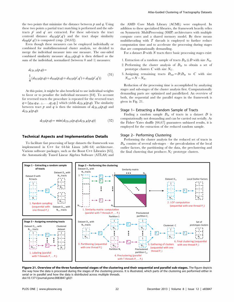
the two points that minimize the distance between p and q. Using
these two points a partial tract matching is performed and the sub-
tracts p’ and q’ are extracted. For these sub-tracts the tract
centroid distance dTCD(p’,q’) and the tract shape similarity
dTSS(p’,q’) is computed (cmp. [50,63]).
Even though these measures can be employed individually or
combined for multidimensional cluster analysis, we decided to
merge the individual measure into one measure. The one-sided
combined similarity measure dCD O(p,q) is then defined as the
sum of the individual, normalized (between 0 and 1) measures:
dCD O(p,q)~
1
4dTCD(p,q)zdTOS(p,q)zdTCD(p0,q0)zdTSS(p0,q0)ð Þ
ð31Þ
At this point, it might be also beneficial to use individual weights
to favor or to penalize the individual measures [64]. To account
for reversed tracts the procedure is repeated for the reversed tract
q~fqM ,qM{1, . . . ,q2,q1g which yields dCD R(p,q). The similarity
between tract p and q is then the minimum of dCD O(p,q) and
dCD R(p,q):
dCD(p,q)~ min dCD O(p,q),dCD R(p,q)ð Þ ð32Þ
Technical Aspects and Implementation Details
To facilitate fast processing of large datasets the framework was
implemented in C++ for 64-bit Linux (x86–64) architecture.
Various software packages, such as the Boost C++ Libraries [65],
the Automatically Tuned Linear Algebra Software (ATLAS) and
the AMD Core Math Library (ACML) were employed. In
addition to these specialized libraries, the framework heavily relies
on Symmetric MultiProcessing (SMP) architectures with multiple
compute cores and a shared memory model. By these means
multithreading with T threads is employed to further reduce
computation time and to accelerate the processing during stages
that are computationally demanding.
For a dataset D with N tracts three basic processing stages exist:
1. Extraction of a random sample of tracts Din(D with size Nin.
2. Performing the cluster analysis of Din to obtain a set of
prototype clusters C with size NC .
3. Assigning remaining tracts Dout~D\Din to C with size
Nout~N{Nin.
Reduction of the processing time is accomplished by analyzing
stages and sub-stages of the cluster analysis first. Computationally
demanding parts are optimized and parallelized. An overview of
both, the sequential and the parallel stages in the framework is
given in Fig. 21.
Stage 1– Extracting a Random Sample of TractsFinding a random sample Din of tracts in a dataset D is
computationally not demanding and can be carried out serially. As
the Fisher–Yates shuffle [66,67] guarantees unbiased results, it is
employed for the extraction of the reduced random sample.
Stage 2– Performing ClusteringPerforming the cluster analysis for the reduced set of tracts in
Din consists of several sub-stages – the precalculation of the local
outlier factors, the partitioning of the data, the preclustering and
the final clustering that produces NC prototype clusters.
Figure 21. Overview of the three fundamental stages of the clustering and their sequential and parallel sub-stages. The figure depictsthe way how the data is processed during the stages of the clustering process. It is illustrated, which parts of the clustering are performed either inserial or in parallel and how the data is distributed across multiple threads.doi:10.1371/journal.pone.0083847.g021
Atlas-Guided Clustering of Tractography Datasets
PLOS ONE | www.plosone.org 22 December 2013 | Volume 8 | Issue 12 | e83847
The computationally most expensive operation is the recurrent
calculation of the pair-wise similarities between all tracts in Din
that is necessary in all stages but the partitioning stage.
Consequently, similarities are computed only once and stored on
disk before LOFs are calculated.
Since the entirety of similarities must be available, (N2in{Nin)=2
similarities are computed for every feature to obtain the triangular
Nin|Nin similarity matrix S. This, however, does not cover the
computational complexity necessary to compute the pair-wise
similarity for two tracts. Employing complex features (e.g.,
Hausdorff distance) will increase the computational complexity
further.
To reduce the computation time, the calculation of the
triangular matrix S is sourced out to multiple threads and
performed in parallel. Matrix S is divided into an arbitrary
number of contiguous line-segments, with an approximately equal
number of tracts (since the matrix is triangular, the number of
elements differ from line to line). All similarities related to one tract
are calculated by one thread.
LOFs are then computed by employing the precalculated
similarities.
For the preclustering, the Fisher–Yates shuffle is employed to
shuffle the tracts in Din, before Din is partitioned into NP sets
P1 . . . PNPwith approximately equal size &Nin=NP. The parti-
tions are then clustered simultaneously. Later on, the final
clustering is carried out serially.
Stage 3– Assigning Remaining TractsSince the remaining tracts in Dout must be assigned to their
individual, most similar prototype clusters of C, the similarity for
each tract p[Dout to all prototype representatives in C has to be
computed by employing the same similarity measures as in stage 2.
The Nout tracts of Dout are partitioned into T segments of
approximately equal size &Nout=T . The segments are assigned to
T threads and similarity computations are carried out in parallel.
Supporting Information
Glossary S1 Glossary that provides short explanationsfor frequently used terms and abbreviations.
(PDF)
Author Contributions
Conceived and designed the experiments: CR DG JRR. Performed the
experiments: CR. Analyzed the data: CR DG. Contributed reagents/
materials/analysis tools: CR DG JRR. Wrote the paper: CR. Discussion of
results: DG MS HJM JRR. Revision of the manuscript: CR DG MS HJM
JRR. Defining the bundles in the white matter atlas: DG MS HJM.
References
1. Le Bihan D, Breton E (1985) Imagerie de diffusion in vivo par resonance
magnetique nucleaire. C R Acad Sci Paris 301: 1109–1112.
2. Leergaard TB, White NS, de Crespigny A, Bolstad I, D’Arceuil H, et al. (2010)
Quantitative histological validation of diffusion MRI fiber orientation distribu-
tions in the rat brain. PLoS One 5: e8595.
3. Mori S, van Zijl PCM (2002) Fiber tracking: principles and strategies - a
technical review. NMR Biomed 15: 468–480.
4. Dauguet J, Peled S, Berezovskii V, Delzescaux T, Warfield SK, et al. (2007)
Comparison of fiber tracts derived from in-vivo DTI tractography with 3D
histological neural tract tracer reconstruction on a macaque brain. Neuroimage
37: 530–538.
5. Basser PJ, Pajevic S, Pierpaoli C, Duda J, Aldroubi A (2000) In vivo fiber
tractography using DT-MRI data. Magn Reson Med 44: 625–632.
6. Conturo TE, Lori NF, Cull TS, Akbudak E, Snyder AZ, et al. (1999) Tracking
neuronal _ber pathways in the living human brain. Proc Natl Acad Sci USA 96:
10422–10427.
7. Mori S, Crain BJ, Chacko VP, van Zijl PC (1999) Three-dimensional tracking of
axonal projections in the brain by magnetic resonance imaging. Ann Neurol 45:
265–269.
8. Parker GJM, Alexander DC (2005) Probabilistic anatomical connectivity derived
from the microscopic persistent angular structure of cerebral tissue. Philos
Trans R Soc Lond B Biol Sci 360: 893–902.
9. Lazar M, Alexander AL (2005) Bootstrap white matter tractography (BOOT-
TRAC). Neuroimage 24: 524–532.
10. Behrens TEJ, Berg HJ, Jbabdi S, Rushworth MFS, Woolrich MW (2007)
Probabilistic di_usion tractography with multiple fibre orientations: What can
we gain? Neuroimage 34: 144–155.
11. Lanyon LJ (2012) Neuroimaging – Methods, InTech, chapter Diffusion Tensor
Imaging: Structural Connectivity Insights, Limitations and Future Directions.
137–162.
12. Stadlbauer A, Nimsky C, Buslei R, Salomonowitz E, Hammen T, et al. (2007)
Diffusion tensor imaging and optimized fiber tracking in glioma patients:
Histopathologic evaluation of tumorinvaded white matter structures. Neuro-
image 34: 949–956.
13. Nucifora PGP, Verma R, Lee SK, Melhem ER (2007) Diffusion-tensor MR
imaging and tractography: exploring brain microstructure and connectivity.
Radiology 245: 367–384.
14. Fillard P, Gilmore J, Piven J, Lin W, Gerig G (2003) Quantitative analysis of
white matter fiber properties along geodesic paths. Medical Image Computing
and Computer-Assisted Intervention-MICCAI 2003 : 16–23.
15. Gong G, Jiang T, Zhu C, Zang Y, Wang F, et al. (2005) Asymmetry analysis of
cingulum based on scale-invariant parameterization by diffusion tensor imaging.
Hum Brain Mapp 24: 92–98.
16. O’Donnell LJ, Westin CF, Golby AJ (2007) Tract-based morphometry. Med
Image Comput Comput Assist Interv 10: 161–168.
17. Ros C, Gullmar D, Stenzel M, Mentzel HJ, Reichenbach JR (2012) Quantitative
_ber bundle-based analysis of diffusion-weighted MRI data. Biomed Tech (Berl)
57: 530–533.
18. Ashburner J, Friston KJ (2000) Voxel-based morphometry – the methods.
Neuroimage 11: 805–821.
19. Smith SM, Jenkinson M, Johansen-Berg H, Rueckert D, Nichols TE, et al.
(2006) Tract-based spatial statistics: voxelwise analysis of multi-subject diffusion
data. Neuroimage 31: 1487–1505.
20. Chao TC, Chou MC, Yang P, Chung HW,Wu MT (2009) Effects of
interpolation methods in spatial normalization of diffusion tensor imaging data
on group comparison of fractional anisotropy. Magn Reson Imaging 27: 681–
690.
21. Wakana S, Jiang H, Nagae-Poetscher LM, van Zijl PCM, Mori S (2004) Fiber
tract-based atlas of human white matter anatomy. Radiology 230: 77–87.
22. Verhoeven JS, Sage CA, Leemans A, Hecke WV, Callaert D, et al. (2010)
Construction of a stereotaxic DTI atlas with full diffusion tensor information for
studying white matter maturation from childhood to adolescence using
tractography-based segmentations. Hum Brain Mapp 31: 470–486.
23. Zhang Y, Zhang J, Oishi K, Faria AV, Jiang H, et al. (2010) Atlas-guided tract
reconstruction for automated and comprehensive examination of the white
matter anatomy. Neuroimage 52: 1289–1301.
24. Wakana S, Caprihan A, Panzenboeck MM, Fallon JH, Perry M, et al. (2007)
Reproducibility of quantitative tractography methods applied to cerebral white
matter. Neuroimage 36: 630–644.
25. Ros C, Guullmar D, Stenzel M, Mentzel HJ, Reichenbach JR (2012) A semi-
automatic approach for the extraction of white matter fiber bundles across
subjects. In: Proc Intl Soc Mag Reson Med. Melbourne, Australia, volume 20.
26. Xu R, Wunsch DC (2008) Clustering. Wiley-IEEE Press.
27. Ding Z, Gore JC, Anderson AW (2003) Classification and quantification of
neuronal fiber pathways using diffusion tensor MRI. Magn Reson Med 49: 716–
721.
28. Brun A, Knutsson H, Park HJ, Shenton ME, Westin CF (2004) Clustering Fiber
Traces Using Normalized Cuts. Lect Notes Comput Sci 3216/2004: 368–375.
29. Moberts B, Vilanova A, van Wijk JJ (2005) Evaluation of Fiber Clustering
Methods for Diffusion Tensor Imaging. In: VIS 05. IEEE. IEEE Computer
Society, p. 9. URL http://doi.ieeecomputersociety.org/10.1109/VIS.2005.29.
30. Huang H, Zhang J, Jiang H, Wakana S, Poetscher L, et al. (2005) DTI
tractography based parcellation of white matter: application to the mid-sagittal
morphology of corpus callosum. Neuroimage 26: 195–205.
31. O’Donnell LJ, Kubicki M, Shenton ME, Dreusicke MH, Grimson WEL, et al.
(2006) A method for clustering white matter fiber tracts. AJNR Am J Neuroradiol
27: 1032–1036.
32. Zhang S, Correia S, Laidlaw DH (2008) Identifying white-matter fiber bundles
in DTI data using an automated proximity-based fiber-clustering method.
IEEE T Vis Comput Gr 14: 1044–1053.
33. Maddah M, Grimson WEL, Warfield SK, Wells WM (2008) A unified
framework for clustering and quantitative analysis of white matter fiber tracts.
Med Image Anal 12: 191–202.
34. Li H, Xue Z, Guo L, Liu T, Hunter J, et al. (2010) A hybrid approach to
automatic clustering of white matter fibers. Neuroimage 49: 1249–1258.
Atlas-Guided Clustering of Tractography Datasets
PLOS ONE | www.plosone.org 23 December 2013 | Volume 8 | Issue 12 | e83847
35. Garyfallidis E, Brett M, Correia MM, Williams GB, Nimmo-Smith I (2012)
QuickBundles, a Method for Tractography Simplification. Front Neurosci 6:175.
36. Wu X, Xie M, Zhou J, Anderson AW, Gore JC, et al. (2012) Globally optimized
fiber tracking and hierarchical clustering – a unified framework. Magn ResonImaging 30: 485–495.
37. Wang Q, Yap PT, Wu G, Shen D (2013) Application of neuroanatomicalfeatures to tractography clustering. Hum Brain Mapp 34: 2089–2102.
38. O’Donnell LJ, Westin CF (2007) Automatic tractography segmentation using a
high-dimensional white matter atlas. IEEE T Med Imaging 26: 1562–1575.39. Visser E, Nijhuis EHJ, Buitelaar JK, Zwiers MP (2011) Partition-based mass
clustering of tractography streamlines. Neuroimage 54: 303–312.40. Guevara P, Poupon C, Rivire D, Cointepas Y, Descoteaux M, et al. (2011)
Robust clustering of massive tractography datasets. Neuroimage 54: 1975–1993.41. O’Donnell LJ, Golby AJ, Westin CF (2013) Fiber clustering versus the
parcellation-based connectome. Neuroimage 80: 283–289.
42. Guha S, Rastogi R, Shim K (2001) Cure: An Efficient Clustering Algorithm forLarge Databases. Inf Syst 26: 35–58.
43. Karypis G, Eui, News VK (1999) Chameleon: Hierarchical Clustering UsingDynamic Modeling. Computer 32: 68–75.
44. Breunig MM, Kriegel HP, Ng RT, Sander J (2000) LOF: Identifying Density-
Based Local Outliers. In: Chen W, Naughton JF, Bernstein PA, editors,SIGMOD Conference. ACM, 93–104. URL http://doi.acm.org/10.1145/
342009.335388.45. Heid O (2000) Eddy Current-Nulled Diffusion Weighting. In: Proc Intl Soc Mag
Reson Med. Denver, Colorado, USA, 8.46. Wang R, Benner T, Sorensen AG, Wedeen VJ (2007) Diffusion Toolkit: A
Software Package for Diffusion Imaging Data Processing and Tractography. In:
Proc Intl Soc Mag Reson Med. Berlin, Germany, 15.47. Avants BB, Tustison NJ, Song G, Cook PA, Klein A, et al. (2011) A reproducible
evaluation of ANTs similarity metric performance in brain image registration.Neuroimage 54: 2033–2044.
48. Jenkinson M, Beckmann CF, Behrens TEJ, Woolrich MW, Smith SM (2012)
FSL. Neuroimage 62: 782–790.49. Ward JH (1963) Hierarchical Grouping to Optimize an Objective Function.
Journal of the American Statistical Association 58: 236–244.50. Ros C, Gullmar D, Reichenbach JR (2010) A new combined distance measure
for the clustering of fiber tracts in Diffusion Tensor Imaging (DTI). In: Proc IntlSoc Mag Reson Med. Stockholm, Sweden, volume 18.
51. Mentzel HJ, Ros C, Gullmar D (2011) Diffusion magnetic resonance
tomography of the brain in childhood. Monatsschr Kinderh 159: 325–332.
52. Drachman DA (2005) Do we have brain to spare? Neurology 64: 2004–2005.
53. Tuch DS (2004) Q-ball imaging. Magn Reson Med 52: 1358–1372.
54. Descoteaux M, Angelino E, Fitzgibbons S, Deriche R (2007) Regularized, fast,
and robust analytical Q-ball imaging. Magn Reson Med 58: 497–510.
55. Descoteaux M, Deriche R, Knosche TR, Anwander A (2009) Deterministic and
probabilistic tractography based on complex fibre orientation distributions.
IEEE Trans Med Imaging 28: 269–286.
56. Guevara P, Duclap D, Poupon C, Marrakchi-Kacem L, Fillard P, et al. (2012)
Automatic _ber bundle segmentation in massive tractography datasets using a
multi-subject bundle atlas. Neuroimage 61: 1083–1099.
57. Yendiki A, Panneck P, Srinivasan P, Stevens A, Zllei L, et al. (2011) Automated
probabilistic reconstruction of white-matter pathways in health and disease using
an atlas of the underlying anatomy. Front Neuroinform 5: 23.
58. Corouge I, Gouttard S, Gerig G (2004) Towards a shape model of white matter
fiber bundles using diffusion tensor MRI. In: IEEE Int Symp Biomed Imag.
IEEE, 344–347.
59. Batchelor PG, Calamante F, Tournier JD, Atkinson D, Hill DLG, et al. (2006)
Quantification of the shape of fiber tracts. Magn Reson Med 55: 894–903.
60. Wassermann D, Bloy L, Kanterakis E, Verma R, Deriche R (2010)
Unsupervised white matter fiber clustering and tract probability map generation:
applications of a Gaussian process framework for white matter fibers.
Neuroimage 51: 228–241.
61. Owens JD, Houston M, Luebke D, Green S, Stone JE, et al. (2008) GPU
Computing. Proceedings of the IEEE 96: 879–899.
62. Ros C, Tandetzky R, Gullmar D, Reichenbach JR (2011) GPGPU-Computing
for the cluster analysis of fiber tracts: Replacing a $15000 high end PC with a
$500 graphics card. In: Proc Intl Soc Mag Reson Med. Montreal, Canada,
volume 19.
63. Attalla E, Siy P (2005) Robust shape similarity retrieval based on contour
segmentation polygonal multiresolution and elastic matching. Pattern Recogn
38: 2229–2241.
64. Gullmar D, Langner J, Haueisen J, Reichenbach JR (2008) Combination of
distance measures for optimal fiber clustering in diffusion tensor imaging. In:
Proc Intl Soc Mag Reson Med. Toronto, Canada, volume 16.
65. Karlsson B (2005) Beyond the C++ Standard Library – An Introduction to
Boost. Addison-Wesley Longman, Amsterdam, 432 pp.
66. Fisher RA, Yates F (1948) Statistical tables for biological, agricultural and
medical research. Oliver & Boyd, 3rd edition.
67. Durstenfeld R (1964) Algorithm 235: Random permutation. Commun ACM 7:
420.
Atlas-Guided Clustering of Tractography Datasets
PLOS ONE | www.plosone.org 24 December 2013 | Volume 8 | Issue 12 | e83847