ATLAS and CMS Statistical methods at University and INFN ...
27
Statistical methods at ATLAS and CMS Michele Pinamonti (ATLAS) University and INFN Roma "Tor Vergata" Higgs Toppings Workshop, Benasque 28 th May - 1 st June 2018
Transcript of ATLAS and CMS Statistical methods at University and INFN ...

Statistical methods at ATLAS and CMS
Michele Pinamonti (ATLAS)University and INFN Roma "Tor Vergata"
Higgs Toppings Workshop, Benasque 28th May - 1st June 2018

Building Likelihoods● Most analyses (especially ttH/tH, with more data available...) are "shape analyses"
○ based on distributions of continuous observables○ signal and background predictions depend on parameters:
■ parameter of interest, POI (e.g. signal strength µ)■ eventually other ("nuisance") parameters, NPs
(e.g. background normalization...)
● Build a global likelihood function:
○ binned likelihood:
○ unbinned likelihood:
● Result = POI value that maximizes the likelihood 2
observed bin contents parameters
S+B prediction in bin i
PDFs for for S and Bvalues of observable m
Poisson
arXiv:1802.04146
arXiv:1804.03682

The Profile Likelihood approach
3
● The profile likelihood is a way to include systematic uncertainties in the likelihood○ systematics included as "constrained" nuisance parameters○ the idea behind is that systematic uncertainties on the measurement of µ come from
imperfect knowledge of parameters of the model (S and B prediction)■ still some knowledge is implied: "θ = θ0 ± Δθ"
○ external / a priori knowledge interpreted as "auxiliary/subsidiary measurement", implemented as constraint/penalty term, i.e. probability density function(usually Gaussian, interpreting "±Δθ" as Gaussian standard deviation)
- usually θ0=0 and Δθ=1 (convention)- define effect of systematic j on prediction x in bin i at "+1" and "-1",- then interpolate & extrapolate for any value of θ
Normalization factors and MC statistics● Beside NP associated to systematic uncertainties,
other NP can be included in the likelihood as free parameters, in the same way as the POI:○ called "normalization factors" (NF)○ no prior, multiplicative factors (⇒ linear) for particular S, B or B components:
B(θ, k) = k⋅ B(θ)
● Statistical uncertainty from limited number of (MC) events used to build the histograms for predicted S and B result in independent uncertainties in each bin, referred to as "MC stat."
○ implemented as additional NPs (one per bin) with scaled Poisson ("gamma") priors○ default: single MC-stat NP assigned to total prediction (S+B) in each bin:
■ problematic for signal, or in general component of the prediction with the POI attached to it (e.g. if these NP get pulled)⇒ NOT applied to signal
■ could consider to split it: useful?
4

Categories, SRs, CRs...● Multiple analysis regions / event categories often used:
○ decay modes○ kinematic selections
● Useful to model these separately if○ sensitivity is better in some regions (avoids dilution)○ some regions can constrain NPs (including NP for systematics)
■ e.g. control regions for backgrounds● Analyse them simultaneously to model correlations
between the regions (common NPs)○ better than a-posteriori combination
● If no statistical correlations (orthogonal)⇒ can simply take likelihood product
● Usually coherent/correlated effect of all parameters (including NP for systematics)in all bins, in all regions
5
Phys. Rev. D 97, 072016

Profile Likelihood maximization● With such a likelihood defined, the measurement of the parameter of interest (POI, or µ)
becomes a N-dimensional likelihood maximisation (or negative-log-likelihood minimization) problem:
N = N(POI) + N(NP)
○ ⇒ N-dimensional fit■ fit result is "best point" (µ, θ)
6

Profile Likelihood Ratio● Neyman-Pearson lemma:
○ the likelihood ratio L(H0)/L(H1) is the optimal discriminator when testing hypothesis H1 vs. H0 - e.g. H1 = presence of signal (µ>0), H0 no signal (µ=0)
● In case of profile likelihood, define profile likelihood ratio (PLR):
● Test statistics defined as: , , ...
● Can then build p-value and significance:
7
distribution of test statistics

Asymptotic regime● In large statistics data samples, the distribution of the test statistic is known
according to Wilks’ Theorem (independently on the prior!):○ χ2 distribution○ parabolic shape around the minimum
⇒ can directly calculate p0 ⇒ significance
⇒ can get the uncertainty on µ
● No need to use pseudo experiments● This theorem holds true for even as few as
~ O(10) events in a data sample8

Profiling, pre-fit and post-fit● Profile likelihood fit can:
○ change background prediction, if best-fit θ values different from θ0 ○ reduce uncertainty on background, through:
■ constraint of NPs ("improved knowledge" of parameters that are affected by systematic uncertainties, i.e. data have enough statistical power to further constraint the NP)
■ correlations between NPs
9
FIT

NP pulls, constraints and correlations● Useful to monitor NP pulls and constraints:
○ they are "nuisance", but they are important!
● Important to consider also NP correlations:○ uncertainties on NPs (and POI) extracted from
covariance matrix, which includes correlation coefficients■ correlation built by the fit, even if completely
independent / uncorrelated sources of uncertainty before the fit(correlation in the improved knowledge of the parameters)
■ (anti-)correlations can reduce total post-fit uncertainty!10
Phys. Rev. D 97, 072003

Impact of NP on the POI● To answer the question "which systematics are more important?"
● The "ranking plot" shows pre-fit and post-fit impact of individual NP on the determination of µ:○ each NP fixed to ± 1 pre-fit and post-fit sigmas (Δθ and Δθ = uncertainty on θ)○ fit re-done with N-1 parameters○ impact extracted as difference in
central value of µ
11
^ ^

Splitting of uncertainties● To answer a similar but different question:
○ how much of the total uncertainty comes from a certain set of systematic uncertainties?○ or similarly, how large is the pure "statistical uncertainty"?
● Procedure:○ fix a group of NPs to post-fit values○ repeat the fit○ look at error on µ this time
and get Δµ as quadratic difference between full and reduced error
○ statistical uncertainty obtained by fixing all NPs
12
arXiv:1804.03682
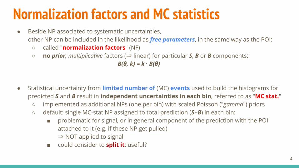
Profiling issues● The profile likelihood approach is valid with some assumptions
○ in particular, assumed that "nature" can be described by the model with a single combination of values for the parameters
● Cannot just take large uncertainties hoping that they are enough to cover for imperfect knowledge of S+B expectation!
● "Flexibility" / "granularity" of the systematics model needs to be considered
13
nominal
syst "up"
syst "down"
This configuration will not be able to fit these points
following this "true" distribution

The constraint issue● Flexibility more and more critical when statistical uncertainty on data becomes
less and less important w.r.t. systematics○ e.g. taking the example before:
● More real examples:○ single JES systematic NP across all jet energy spectrum allows high-stats low-energy control
regions/bins to calibrate JES for high energy jets → intended?○ simple ± 50% overall uncertainty on tt+jets background, probably enough to cover
uncertainties also in remote phase-spaces (tails of distributions for tt+HF-enriched selection), but data in tt+light-jets-enriched CRs will constrain it to <5%, propagated to SRs... → ok?
14
constraint by high stat. bins new physics!?
... no, data just following background real distribution...

Theory modeling systematics● Experimental systematics nowadays often well suited for profile likelihood application:
○ come from calibrations ⇒ gaussian constraint appropriate○ broken-down into several independent/uncorrelated components (JES, b-tagging...)
● Different situation for theory systematics:○ difficulty 1: what is the distribution of the subsidiary measurement?○ difficulty 2: what are the parameters of the systematic?
■ can a combination of the included parameters describe any possible configuration?■ is any allowed value of the parameter physically meaningful?
● The obviously tricky case: "two point" systematics○ e.g. Herwig vs. Pythia as "parton shower and
hadronization model uncertainty",as a single NP
15
See: https://indico.cern.ch/event/287744/contributions/1641261/attachments/535763/738679/Verkerke_Statistics_3.pdf

Theory modeling systematics
16
One-bin case:- reasonable to think that "Sherpa"
can be between Herwig and Pythia
Shape case:- Sherpa can be different from linear
combination of Py and Her...
Which prior?
Pre-fit / non-constrained NP could be fine to cover for all possible models...
... but is this level of constraint ok?

Theory modeling systematics● A not-so-obviously tricky case:
○ scale uncertainties
17
Take NLO scale variations as uncertainty (missing NNLO MC)
+1
-1
⇒ flat uncertainty here, and NNLO is within uncertainty, but NNLO/NLO is not flat!
Suppose data looks like NNLO, we measure ytt, we constrain scale syst. in low ytt bins ⇒ new physics at high ytt?
Phys. Rev. Lett. 116, 082003

Systematics model validation● Especially given the impossibility to build a "perfect model", need to validate flexibility of
the adopted systematics model (better if before looking at the full data!)
● Response of the model to injection tests:○ build toy data (or Asimov data) with non-nominal properties
■ can vary parameters of the model (i.e. by shifting NPs when creating the Asimov data-set)
■ can use a MC generator not included in the systematics model to build the toy data
■ check compatibility of best-fit POI with injected value
● Post-fit plots:○ evaluate data/prediction agreement across distributions with fit result projection
(shifted prediction + reduced systematics band)○ can spot issues e.g. if found disagreement in a region where don't expect signal○ especially useful for validation regions / validation distributions
i.e. regions / distributions not directly used in the fit
● Mention for sure the test with modified Asimov dataset (from alternative MC sample for one or more backgrounds, not used in the definition of systematics model)
○ very useful to probe the flexibility of the fit model
18
Fit Fit FitAsimov
S+BAsimov'
S+B(θ=θ') Asimov''
S+B'
^µ = 1
^µ'
^µ''

Statistical fluctuations on systematics● Often systematic uncertainty definition affected by statistical uncertainty
○ typical example again from two-point systematics, evaluated as the difference between two statistically independent MC samples, and at least one of them statistically limited
● Current PLR formalism doesn't account for this effect:effect of ±Δθj on S and B assumed to be known with no uncertainty
○ ongoing efforts (in ATLAS at least) to try to incorporate this, e.g. adding NPs for size of ΔBij = [ Bi(θj=1) - Bi(θj=0) ] → ΔBij
0 ± Δ(ΔBij) = ΔBij0 + νij ...
● To assess the size of the effect:○ can use pseudo-experiments / toys (e.g. with bootstrap method)
■ repeat measurement N times and see distribution of Δµ
● To mitigate the effect:○ ATLAS uses smoothing of systematic variations in single distributions
■ assumption of "regular" shape of systematic variation19
new NPs

Including data-driven estimates into the fit model● Often data-driven estimates provided as inputs for the PLR model
○ however, ideally better to include the estimate in the fit model■ easier handling of correlations■ natural way of considering signal contamination in control region
○ not always possible/easy (example: Matrix Method for fakes and non-prompt lepton background determination)
● With more and more data, natural to consider more and more data-driven or partially data-driven background estimation techniques, also for backgrounds currently estimated through MC and with NPs constrained by the data
○ by building more data-driven predictions, possibly included in the PLR model, could reduce issues related to over-constraints of NPs and enhance model flexibility
20
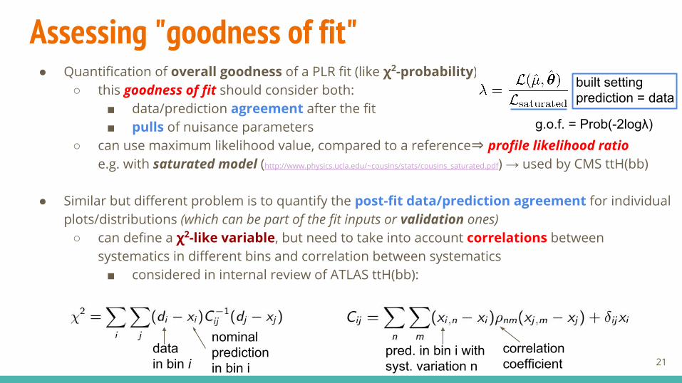
Assessing "goodness of fit"● Quantification of overall goodness of a PLR fit (like χ2-probability)
○ this goodness of fit should consider both:■ data/prediction agreement after the fit■ pulls of nuisance parameters
○ can use maximum likelihood value, compared to a reference⇒ profile likelihood ratioe.g. with saturated model (http://www.physics.ucla.edu/~cousins/stats/cousins_saturated.pdf) → used by CMS ttH(bb)
● Similar but different problem is to quantify the post-fit data/prediction agreement for individual plots/distributions (which can be part of the fit inputs or validation ones)
○ can define a χ2-like variable, but need to take into account correlations between systematics in different bins and correlation between systematics
■ considered in internal review of ATLAS ttH(bb):
21data in bin i
nominal prediction in bin i
correlation coefficient
pred. in bin i with syst. variation n
g.o.f. = Prob(-2logλ)
built setting prediction = data

Combination of measurements● With the PLR approach, combination of different
measurements is natural:○ "just" add some more bins to the product
● However, important to consider compatibility of models:○ orthogonality of channels:
■ bin contents in PLR are supposed to be statistically independent
○ same definition of (set of) POI:■ sometimes obvious, but not always
(is µ applied to all the ttH, or just one decay channel? What about tH? ...)○ compatible set of systematics:
■ this is the most tricky part, especially for ATLAS+CMS combinations!■ mainly dealing with the question "which NPs are correlated between channels?"■ often cannot reach perfect solution, need to test different correlation assumptions
(notice that in PLR formalism systematics are either fully correlated or fully uncorrelated...)22

Summary and conclusions● Profile likelihood ratio (PLR) approach presented, in the context of ttH analyses
(mainly in the "binned case", i.e. ttH(bb) and multi-lepton channels)○ tod, mefeatures and possible pitfalls discussed
● Room for fruitful discussion on the most critical points in these days○ important to consider how the current approach will work and eventually evolve with:
■ more and more data■ more and more precision measurements■ more and more accurate/refined/rich theory predictions■ new experimental analysis techniques...
23

Backup
24

NP interpolation / extrapolation● The "NP interpolation / extrapolation" controls how a variation of a NP θj reflects in a
variation of the predicted yields (S(θj) and B(θj), in the various bins)● Different schemes / codes are implemented in RooStats/RooFit, e.g.:
○ piecewise linear → default for shape component of systematics○ polynomial interpolation / exponential extrapolation → default for norm. component
θ θ
B(θ) B(θ)
25
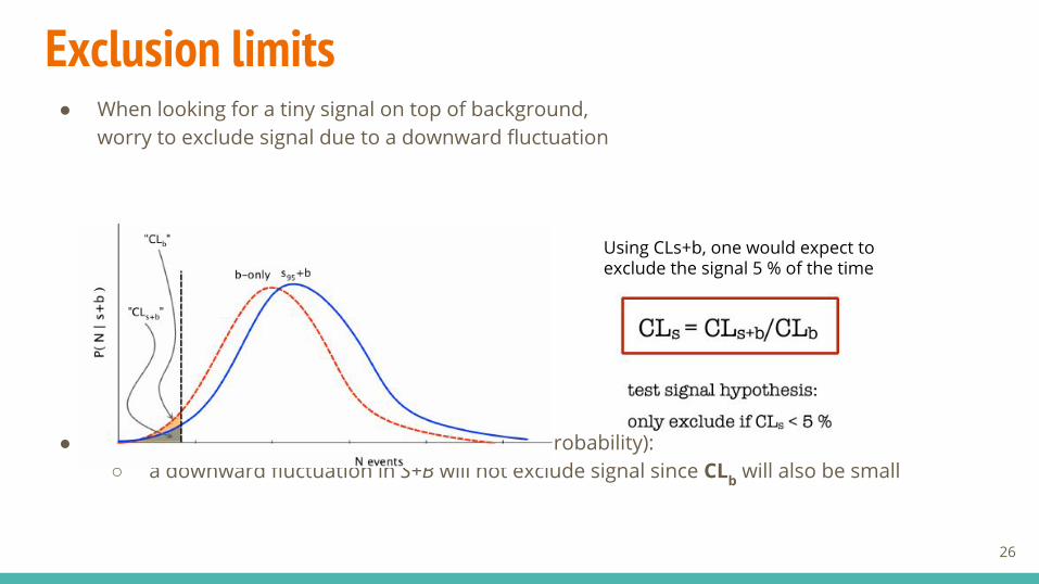
Exclusion limits● When looking for a tiny signal on top of background,
worry to exclude signal due to a downward fluctuation
● So we use CLs to test a signal hypothesis (not a probability):○ a downward fluctuation in S+B will not exclude signal since CLb will also be small
Using CLs+b, one would expect toexclude the signal 5 % of the time
26

Implementation (in ROOT)● RooFit: toolkit to extend ROOT providing language to describe data models
○ model distribution of observable x in terms of parameters θ using probability density function PDF
● RooStats: project to provide advanced stat. techniques for LHC collaborations○ built on top of RooFit
● RooWorkspace: generic container class for all RooFit objects, containing:○ full model configuration
(i.e. all information to run statistical calculations)○ PDF and parameter/observables descriptions uncertainty/shape of nuisance parameters○ (multiple) data sets
● HistFactory: tool for creating RooFit workspaces formatted for use with RooStats tools○ meant for analyses based on template histograms
27