Draft version February 9, 2016Preprint typeset using LATEX style emulateapj v. 08/22/09

SDSS-II SUPERNOVA SURVEY: AN ANALYSIS OF THE LARGEST SAMPLE OF TYPE IA SUPERNOVAEAND CORRELATIONS WITH HOST-GALAXY SPECTRAL PROPERTIES

Rachel C. Wolf1, Chris B. D’Andrea2,3, Ravi R. Gupta1,4, Masao Sako1, John A. Fischer1, Rick Kessler5,Saurabh W. Jha6, Marisa C. March1, Daniel M. Scolnic5, Johanna-Laina Fischer1, Heather Campbell3,7,

Robert C. Nichol3, Matthew D. Olmstead8,9, Michael Richmond10, Donald P. Schneider11,12, Mathew Smith2,13

Draft version February 9, 2016

ABSTRACT

Using the largest single-survey sample of Type Ia supernovae (SNe Ia) to date, we study the relation-ship between properties of SNe Ia and those of their host galaxies, focusing primarily on correlationswith Hubble residuals (HR). Our sample consists of 345 photometrically-classified or spectroscopically-confirmed SNe Ia discovered as part of the SDSS-II Supernova Survey (SDSS-SNS). This analysisutilizes host-galaxy spectroscopy obtained during the SDSS-I/II spectroscopic survey and from anancillary program on the SDSS-III Baryon Oscillation Spectroscopic Survey (BOSS) that obtainedspectra for nearly all host galaxies of SDSS-II SN candidates. In addition, we use photometric host-galaxy properties from the SDSS-SNS data release (Sako et al. 2014) such as host stellar mass andstar-formation rate. We confirm the well-known relation between HR and host-galaxy mass and finda 3.6σ significance of a non-zero linear slope. We also recover correlations between HR and host-galaxy gas-phase metallicity and specific star-formation rate as they are reported in the literature.With our large dataset, we examine correlations between HR and multiple host-galaxy propertiessimultaneously and find no evidence of a significant correlation. We also independently analyze ourspectroscopically-confirmed and photometrically-classified SNe Ia and comment on the significance ofsimilar combined datasets for future surveys.Subject headings: cosmology: observations — supernovae: general — surveys – galaxies:abundances

1. INTRODUCTION

Type Ia supernovae (SNe Ia) are crucial observationalprobes for investigating the history of our expanding uni-verse. The origin of these phenomena remains a mystery,although there is evidence for two distinct SN Ia progen-itor systems (the so-called single degenerate and doubledegenerate scenarios) that result in a thermonuclear ex-plosion occurring as the mass of a carbon-oxygen whitedwarf approaches the Chandresekhar limit (Whelan &

Electronic address: rcane@physics.upenn.edu1 Department of Physics and Astronomy, University of Pennsyl-

vania, 209 South 33rd Street, Philadelphia, PA 19104, USA2 School of Physics and Astronomy, University of Southampton,

Southampton, SO17 1BJ, UK3 Institute of Cosmology and Gravitation, University of

Portsmouth, Dennis Sciama Building, Burnaby Road, Portsmouth,PO1 3FX, UK

4 Argonne National Laboratory, 9700 South Cass Avenue,Lemont, IL 60439, USA

5 The University of Chicago, The Kavli Institute for Cosmolog-ical Physics, 933 East 56th Street, Chicago, IL 60637, USA

6 Department of Physics and Astronomy, Rutgers, the StateUniversity of New Jersey, 136 Frelinghuysen Road, Piscataway, NJ08854, USA

7 Institute of Astronomy, University of Cambridge, MadingleyRoad, Cambridge CB3 0HA, UK

8 Department of Chemistry and Physics, Kings College, Wilkes-Barre, PA 18711, USA

9 Department of Physics and Astronomy, University of Utah,Salt Lake City, UT 84112, USA

10 School of Physics and Astronomy, Rochester Institute ofTechnology, Rochester, New York 14623, USA

11 Department of Astronomy and Astrophysics, The Pennsylva-nia State University, University Park, PA 16802, USA

12 Institute for Gravitation and the Cosmos, The PennsylvaniaState University, University Park, PA 16802, USA

13 Department of Physics, University of the Western Cape, CapeTown, 7535, South Africa

Iben 1973; Nomoto 1982; Iben & Tutukov 1984; Web-bink 1984; Hillebrandt & Niemeyer 2000). Observationsof these incredibly bright explosions, visible out to highredshifts, have provided evidence for the accelerating ex-pansion of the universe (Riess et al. 1998; Perlmutter et.al. 1999) and are used to measure cosmological parame-ters with increasing precison (Astier et al. 2006; Kessleret al. 2009a; Conley et al. 2011; Betoule et al. 2014; Scol-nic et al. 2014b). Their efficacy as “standard candles”,however, relies on the ability to calibrate intrinsic lumi-nosity with SNe light-curve width (‘stretch’) and opticalcolor (Phillips 1993; Hamuy et al. 1996; Riess et al. 1996;Tripp 1998). After applying these corrections using light-curve fitting techniques, there remains a 1σ dispersion inpeak brightness of about 0.1 magnitudes, correspondingto about five percent in distance (Betoule et al. 2014;Conley et al. 2011). The origin of this scatter remainsunknown; yet it is postulated that both the progenitorand its environment play a role (Gallagher et al. 2005,2008; Neill et al. 2009; Howell et al. 2009; Kelly et al.2010).

Standardization of SNe Ia luminosity can be improvedby searching for additional parameters that correlatewith the Hubble Residual (HR), which quantifies the dif-ference in the distance modulus, corrected for stretchand color, and what is predicted by the best-fit cos-mology. Gallagher et al. (2005) studied the host-galaxyproperties of nearby SNe Ia and found a tenuous corre-lation between the HR and host-galaxy gas-phase metal-licity. More recently, Kelly et al. (2010), Sullivan et al.(2010), and Lampeitl et al. (2010), using independentdata sets, demonstrated that SNe Ia in more massivehosts are about ∼ 0.1 magnitudes brighter (after light-curve corrections) than those in lower mass hosts. Un-

arX

iv:1

602.

0267

4v1

[as

tro-

ph.C

O]

8 F

eb 2

016

2 Wolf et al.

derstanding this relation is crucial for future precisioncosmology experiments. In the recent literature, therehave been several studies indicating that rather than acontinuous linear slope, the HR trend with host stellarmass behaves more like a “step” function, which has atransition region connecting the two levels (Childress etal. 2013; Johansson et al. 2013; Rigault et al. 2013). Thistrend has become known as the “mass step.”

Childress et al. (2013, hereafter C13) combined theirsample of SNe Ia from the Nearby Supernova Factorywith SNe Ia from the literature (namely, Kelly et al. 2010,Sullivan et al. 2010, and Gupta et al. 2011) to create asample of 601 SNe Ia spanning low and high redshift.They used this combined sample to analyze the trendbetween HR and host-galaxy mass and found that thestructure of the trend is consistent with a plateau atlow and high mass separated by a transition region fromlog(M/M) = 9.8 to log(M/M) = 10.4. Several phys-ical models for this behavior were expounded and com-pared to the data, and the authors concluded that thecause of the trend may be due to a combination of theshape of the galaxy mass-metallicity relation, the evolu-tion of SN Ia progenitor age along the galaxy mass se-quence, and the uncertain effects of SN color and hostgalaxy dust.

Johansson et al. (2013, hereafter J13) analyzed a sam-ple of 247 SDSS SNe Ia using only SDSS host-galaxy pho-tometry. They found that, as in C13, the HR-mass rela-tion behaves as a sloped step function, with essentiallyzero slope at the high- and low-mass ends and a non-zero slope in the region 9.5 < log(M/M) < 10.2. Theyreported that the step in the HR-mass plane is close tothe evolutionary transition mass of low-redshift galaxiesfirst described by Kauffmann et al. (2003a). This tran-sition mass occurs at log(M/M) ∼ 10.5 and signifiesa change in galaxy morphology and stellar populations.J13 concluded that differences between SN Ia progeni-tors in these populations could imply the existence oftwo samples of SNe Ia with high and low HR.

Following on the work of C13, Rigault et al. (2013)used integral field spectroscopy for a sample of 89 SNe Iafrom the Nearby Supernova Factory to measure Hα emis-sion within a 1 kpc radius around each SN. This Hαsurface brightness was used to define SN environmentsas either “locally star-forming” or “locally passive” andthey found that the mean standardized brightness forSNe Ia with local Hα emission is on average 0.09 magni-tudes fainter than for those without. They found a bi-modal structure in HR, and claim that the intrinsicallybrighter mode, exclusive to locally passive environments,is responsible for the mass step. They argue that HRsare highly dependent on local environment, with localHα emission being more fundamental than global hostproperties.

There is no known mechanism by which the mass ofthe host galaxy can directly influence the explosion of asingle white dwarf; therefore, other host properties thatare correlated with galaxy mass must be invoked to ex-plain the underlying physical mechanism of this relation.For example, host galaxy gas-phase metallicity is widelyassumed to be a proxy for progenitor metallicity, andthere are models suggesting that SN Ia luminosities de-pend on the stellar metallicity of the progenitor (Timmeset al. 2003; Kasen et al. 2009). Therefore, correlations

between host metallicity and SN properties have beenof recent interest as well. D’Andrea et al. (2011, here-after D11) used a complete sample of all 34 SNe Ia withz < 0.15 detected by the Sloan Digital Sky Survey-II SNSurvey (hereafter SDSS-SNS; Frieman et al. 2008) andcorresponding host-galaxy spectra and found significantcorrelations between gas-phase metallicity and specificstar formation rate with HR. Similar trends were ob-served by C13 and Pan et al. (2014, hereafter P14) usingdata from the SNFactory and PTF, respectively. Kon-ishi et al. (2011) also analyzed host spectra of SDSS SNeand concluded that SNe Ia in metal-rich galaxies are 0.13magnitudes brighter after correcting for light-curve widthand color. Given that broadband photometry of galax-ies is more readily available than galaxy spectra, severalstudies have estimated host galaxy physical propertiesfrom photometry. Gupta et al. (2011) used 206 SNe Iafrom the SDSS-SNS and host-galaxy multi-wavelengthphotometry and found that while the relation of HR withhost stellar mass was highly significant, the relation withmass-weighted age of the host was not. Building on thiswork, Hayden et al. (2013) calibrated the fundamentalmetallicity relation (FMR) of Mannucci et al. (2010) tobetter estimate host metallicity from photometry, andfound that using the FMR improves HR correlation be-yond the stellar mass alone. More recently, using empir-ical models of galaxy star formation histories and theo-retical SN delay time distribution models, Childress etal. (2014) have argued that the mean ages of SNe Ia pro-genitors are responsible for driving the HR correlationwith host mass.

Many recent studies (D11, C13, P14), utilize host-galaxy spectroscopy to study these relations. Campbellet al. (2015, submitted) use SNe Ia from SDSS to ex-plore correlations with spectroscopic host-galaxy proper-ties, using published BOSS data products from the SDSSDR10 catalog (Ahn et al. 2014) and focusing on cos-mological constraints. Using spectroscopy rather thanphotometry provides direct access to the galaxy SEDand a better estimate of dust extinction. It also al-lows for derivations of the gas-phase metallicity and star-formation rates via narrow emission lines. In this work,we study the relationship between SN Ia HRs and proper-ties of their host galaxies, including metallicity and star-formation rate, using SN data from the full three-yearSDSS-SNS (Sako et al. 2014, hereafter S14) and a combi-nation of host-galaxy spectra from an ancillary programof the SDSS-III Baryon Oscillation Spectroscopic Sur-vey (BOSS) (Olmstead et al. 2014; Dawson et al. 2013)and from the SDSS I/II spectroscopic survey (Abazajianet al. 2009; Strauss et al. 2002). In comparison to re-cent literature, this is the largest single-survey sample ofspectroscopically-confirmed or photometrically-classifiedSN Ia light curves and host-galaxy spectroscopic data.As newer, larger surveys, such as the Dark Energy Sur-vey (Bernstein et al. 2012), Pan-STARRS (Kaiser et al.2002), and LSST (LSST Science Collaboration 2009) willalso heavily rely on photometrically-classifed samples ofSNe Ia, the biases and selection effects discussed in thiswork will be critical for future host-galaxy studies.

In this paper we adopt the best-fit flat, ΛCDMcosmology for SNe Ia alone as determined by Betouleet al. (2014, hereafter B14), a joint analysis of 740spectroscopically-confirmed SNe Ia from a compilation of

3

surveys of low, intermediate, and high redshift ranges(ΩM = 0.295). The B14 sample combines 242 high-zSNe Ia from the first 3 years of the Supernova LegacySurvey (SNLS) and 374 SNe Ia from the full 3-year datarelease of SDSS-SNS (0.05 < z < 0.4). The remainder ofthe SN Ia sample are from a collection of low-z surveys,with most from the third release (Hicken et al. 2009)of photometric data acquired at the F. L. Whipple Ob-servatory of the Harvard-Smithsonian Center for Astro-physics (CfA3). Since the value of the Hubble constantis degenerate with the absolute magnitude of SNe Ia, weadopt H0 = 70 km s−1 Mpc−1. We use this cosmologyto compute HR, defined as HR ≡ µSN−µz, where µSN isthe distance modulus estimated from fitting SN Ia lightcurves and µz is the distance modulus computed usingthe redshift and our assumed cosmology. The HR quanti-fies whether our SNe Ia are over-luminous (negative HR)or under-luminous (positive HR) after light-curve correc-tion.

The general structure of this work is as follows: InSection 2 we describe our SN and galaxy data. Section 3highlights light-curve quality requirements for our SNe Iasample and describes the treatment of effects such asMalmquist bias. Section 4 details our methods for ex-tracting galaxy spectroscopy and the selection cuts weimpose on our host galaxy sample. Section 5 outlineshow we derive host galaxy properties from emission-linefluxes. The sample selection requirements discussed inSections 3, 4, and 5 ultimately yield our two final sam-ples for analysis, which contain 345 and 144 SNe Ia, re-spectively. In Section 6 we present our findings and wediscuss our results in Section 7.

2. OBSERVATIONAL DATA

Observations from the SDSS-SNS were used for ourSN Ia sample and a combination of spectra from SDSSand BOSS were utilized for host-galaxy spectroscopy.Spectra of host galaxies are important not only for se-curing redshifts of their SNe, but also as probes of thephysical properties of galaxies themselves. As summa-rized in the previous section, these properties can influ-ence the SN Ia progenitor and the subsequent explosion.We describe how we obtain our SN and host galaxy datain Sections 2.1 and 2.2, respectively.

2.1. Supernovae

All SNe in this work were discovered and observed bythe SDSS-SNS. Data were collected over a three monthobserving season (September - November) in 2005, 2006,and 2007 using the wide-field SDSS CCD camera (Gunnet al. 1998) on the 2.5 meter SDSS telescope at theApache Point Observatory in New Mexico (Gunn et al.2006). The survey observed Stripe 82, a 300 deg2 equa-torial region of the Southern sky, in drift-scan mode, ob-taining nearly simultaneous 55 second exposures in eachof the ugriz SDSS filters (Fukugita et al. 1996). Descrip-tions of the SDSS absolute photometric calibration arefound in Ivezic et al. (2007), Padmanabhan et al. (2008),and Betoule et al. (2013). The average cadence of the sur-vey, including losses due to weather and sky brightness,was ∼ 4 days. Selection of the supernova candidates isdescribed in Sako et al. (2008). High quality light curveswere obtained (Holtzman et al. 2008) with optical pho-tometry that is internally consistent to ∼ 1% (Ivezic et

al. 2007). For a technical summary of the SDSS, see Yorket al. (2000).

A full description of data acquisition and reductionfrom the SDSS-SNS can be found in the final Data Re-lease paper (S14). Over its three-year run, the SDSS-SNS discovered 10,258 new variable objects in the red-shift range 0.01 < z < 0.55. Of these, 499 werespectroscopically-classified as SNe Ia (‘Spec-Ia’). In S14,these SNe Ia are typed “SNIa”.

Analyses that use spectroscopically-identified samplesof SNe Ia (e.g., Kessler et al. 2009a; Betoule et al. 2014)are highly pure, as they contain, to high confidence, onlySNe Ia. However such samples, as in the case of theSDSS-SNS, can be biased, as the likelihood of an SN Iabeing spectroscopically-classified is a function of manyfactors: its location within the host galaxy, its relativebrightness compared to the surface brightness of the hostgalaxy, and its color (but not the intrinsic brightness;see Figure 10 of S14). Additionally, the expense of spec-troscopy is a limiting factor in rolling supernova surveyssuch as the SDSS-SNS: resources are typically unavail-able (or observing conditions disadvantageous) for a com-plete spectroscopic program. For these reasons, we alsouse in this paper SDSS-SNS transients that have beenphotometrically-classified, using the host-galaxy spectro-scopic redshift as a prior, as SNe Ia (‘Phot-Ia’). In S14,these SNe Ia are typed “zSNIa”. We describe the classi-fication and data-quality cuts applied to this catalog oftransients in Section 3.

2.2. Host Galaxies

Our primary source of SN host-galaxy spectroscopy isthe BOSS survey of SDSS-III (Eisenstein et al. 2011).BOSS, which ran from 2008 to 2014, was designed tomeasure the scale of baryon acoustic oscillations (BAO)by observing 1.5 million galaxies to redshift z < 0.7 and150,000 quasars at redshifts 2.15 < z < 3.5 over an areaof 10, 000 deg2. To accommodate this survey, the origi-nal SDSS spectrograph was rebuilt with smaller fibers (2′′

diameter, allowing a larger number of targets per point-ing), more sensitive detectors in both the blue and redchannels, and a wider wavelength range (361−1014 nm).These improvements allowed the survey to reach highergalaxy redshifts and observe about one magnitude deeperthan SDSS. A detailed description of the BOSS spectro-graph (as the upgraded instrument is now known) canbe found in Smee et al. (2013).

Approximately 5% of the BOSS fibers were allocatedto ancillary science programs, one of which was the sys-tematic targeting of host galaxies of SN candidates fromthe SDSS-SNS. Targets for this program were prioritizedbased on the probability of the observed transient be-ing a type Ia or core-collapse SN using the photometric–classification software PSNID (see Section 3), as wellas on the r -band fiber-magnitude of the host galaxy(rfiber < 21.25). A total of 3,761 of the 4,777 requestedtargets were observed, with non-observations primarilydue to the finite availability of fibers and clashes withhigher priority targets. The SDSS-SNS target selectionfor this ancillary program is detailed in Olmstead et al.(2014) and Campbell et al. (2013).

We use in this analysis the host-galaxy matching donein S14. Here each detected transient is matched to theSDSS Data Release 8 (Aihara et al. 2011) catalog us-

4 Wolf et al.

ing an algorithm that identifies the “nearest” galaxy in aparameter space that accounts for the apparent size andsurface brightness profile of each galaxy within a 30′′ ra-dius of the transient coordinates. It is estimated that thismethod is able to match host galaxies with 97% accuracy(S14).

The host-galaxy matching that defined the target se-lection for BOSS spectroscopy was performed years priorto the development of the algorithm used in S14. There-fore, it would not be unexpected if some fraction ofthe BOSS targets do not correspond to the currently-identified host galaxy, resulting in an incorrect assumedredshift for some SNe. We find that the existing red-shifts (either from the SN spectrum or from a non-BOSShost spectrum) of three SNe Ia disagree with those oftheir respective BOSS targets. For each of these cases,the BOSS spectrum is of a galaxy that is offset fromthe currently identified host by more than 8′′, indicatingthat the BOSS target is not the correct host. To avoidpossible ambiguity, we remove these three SNe from oursample. For further discussion of BOSS targeting andhost-galaxy mismatches see S14.

As all of Stripe 82 lies within the area observed by theSDSS-I/II spectroscopic survey, many of our transientshave pre-existing host spectra. The BOSS ancillary pro-gram targeted the location of the SN within the galaxywhere spectroscopy of the host galaxy already exists inthe SDSS database. This paper derives global spectro-scopic properties of the host galaxies, and thus preferen-tially uses SDSS spectra where they exist, as these spec-tra typically have higher S/N than BOSS spectra due totheir larger fiber width (3′′ diameter) and being centeredon the host galaxy.

We will return to this point briefly in Section 5, wherewe discuss the breakdown of spectra passing various cutsfor data quality.

3. SUPERNOVA SELECTION AND PROPERTIES

We select our sample of photometrically-classifiedSNe Ia using the Photometric SN IDentification (PSNID)software (Sako et al. 2011) described in S14. PSNIDuses the observed photometry of the SNe to first com-pute a Bayesian probability associated with each of theassumed three SN types (SN Ia, SN Ibc, and SN II), aswell as parameters and errors assuming a SN Ia model,using a Markov Chain Monte Carlo. The same proce-dures are then performed on a large simulated mixtureof SN Ia and core-collapse SNe. For each SN candidatein our sample, the measured SN Ia parameters (extinc-tion, light-curve stretch, and redshift) are compared withthose of the simulated set to calculate Cartesian dis-tances to its neighbors which are used then to determinea nearest-neighbor probability. The combination of theχ2-fit, Bayesian, and nearest-neighbor probabilities areused for the final classification.

In this work we use only those classifications from S14where the host-galaxy redshift is included as a prior onthe light-curve fit, which is important for precise place-ment of SNe Ia on the Hubble Diagram. We impose thePSNID selection criteria outlined in Section 4 of S14: thePSNID fit probability is ≥ 0.01 for the SN Ia model; theBayesian probability of being an SN Ia is ≥ 0.9; and thenearest-neighbor probability of being an SN Ia is greaterthan that of being a core-collapse SN. We place an addi-

tional requirement on light-curve sampling, requiring thecandidate to have at least one detection at −5 ≤ Trest ≤+5 days and one at +5 < Trest ≤ +15 days, where Trest

is the rest-frame time such that Trest = 0 corresponds topeak brightness in rest-frame B band. Imposing thesecriteria yields a sample of 824 photometrically-classifiedSNe Ia with a purity and efficiency of ∼ 96% (determinedfrom simulations; for more complete definitions of samplepurity and efficiency see S14).

The photometrically-classified SNe selected by theabove requirements, combined with the 499 Spec-Ia, de-fine a maximally large sample of SNe Ia in SDSS-SNS.As we are interested in host-galaxy correlations with thederived distance modulus to these SNe, we apply addi-tional cuts to create a sample that can produce reliabledistance estimates. We fit these light curves using theimplementation of SALT2 (Guy et al. 2010) in the Super-Nova ANAlysis package (SNANA; Kessler et al. 2009b),keeping only SNe Ia that meet the following criteria:

1. At least one detection before peak brightness(Trest < 0).

2. At least one measurement with Trest > +10 days.

3. At least five detections between −15 < Trest < +60days.

4. At least three filter-epoch detections with S/N > 5.

5. The measured color (c) and stretch (x1) are withinthe elliptical cut outlined in Campbell et al. (2013,Figure 6).

6. PFIT > 0.01 where PFIT is the SALT2 light-curve fitprobability based on the χ2.

Distance moduli are then estimated using the codeSALT2mu (Marriner et al. 2011), also a part of the SNANAsuite. In the SALT2 model, the distance modulus is givenby

µSN = mB −M0 + αx1 − βc, (1)

where mB (peak apparent B-band magnitude), x1, andc are fit for each individual SN and M0 (absolute mag-nitude), α, and β are global parameters of the SN sam-ple. SALT2mu computes α and β (cosmology-independentcorrections for the light-curve stretch and color) from agiven SN Ia sample, allowing us to determine µSN for eachSN in the sample.

This computation of the distance modulus, how-ever, has not been corrected for selection effects (i.e.Malmquist Bias). The well-known Malmquist bias(Malmquist 1936) stipulates that for a magnitude limitedsurvey, a given SN Ia may appear brighter due to randomstatistical fluctuations. These fluctuations can be seen toa greater distance and thus a larger portion will be de-tected in a magnitude-limited sample. To determine thecorrection for this effect, as well as others correctionsstemming from SALT2 fitting (e.g., poor fits to low S/Ndata), we run SDSS-like simulations (with approximatelyten times the data statistics) and compare the expected(µTRUE) and observed (µFIT) distance moduli. Realisticlight curves are simulated using the SNANA code, wherethe MC is used to make detailed comparisons with thedata using different models of intrinsic SN Ia brightness

5

0.0 0.1 0.2 0.3 0.4 0.5

0

50

100

150

200

0.0 0.1 0.2 0.3 0.4 0.5

Redshift

0

50

100

150

200N

um

be

r S

Ne

Ia

-0.3 -0.2 -0.1 0.0 0.1 0.2 0.3

0

50

100

150

200

-0.3 -0.2 -0.1 0.0 0.1 0.2 0.3

SALT2 c

0

50

100

150

200

Nu

mb

er

SN

e I

a

-3 -2 -1 0 1 2 3

0

50

100

150

-3 -2 -1 0 1 2 3

SALT2 x1

0

50

100

150

Nu

mb

er

SN

e I

a

Fig. 1.— Comparison of MC simulation (red histogram) andSDSS-SNS data (black points). The MC distributions are normal-ized to the low-z (z < 0.25) data. Error bars on the data pointsrepresent the square root of the number of SNe Ia in the respectivebin. Distributions are displayed for the redshift (top), SALT2 color(middle) and SALT2 stretch (bottom).

variations (Kessler et al. 2013). The simulations assumethe best-fit flat ΛCDM cosmology of B14 (ΩM = 0.295)and SN Ia are generated using the SALT-II model (Guyet al. 2010). As in Kessler et al. (2013), we simulateasymmetric Gaussian distributions for our input colorand stretch. The following parameters best match ourdata: c = −0.09, σ+,c = 0.13, σ−,c = 0.02, x1 = 0.5,σ+,x1

= 0.5, and σ−,x1= 1.5. Comparisons between the

data and simulations are presented in Figure 1.The average difference in distance modulus as a func-

tion of redshift, which we define as µBIAS, is presented in

0.0 0.1 0.2 0.3 0.4 0.5

−0.08

−0.06

−0.04

−0.02

0.00

0.02

0.0 0.1 0.2 0.3 0.4 0.5Redshift

−0.08

−0.06

−0.04

−0.02

0.00

0.02

µB

IAS (

<µ

FIT −

µT

RU

E>

)

Fig. 2.— Difference between the measured and true distancemodulus (defined as µBIAS) from our simulations, as a functionof redshift. Data points are inverse-variance weighted averages inredshift bins of width 0.025 with error bars representing the widthof each bin. Each bin contains at least 500 SNe Ia.

TABLE 1Cumulative PM Sample Definition

Selection Requirements Removed Total Phot-Ia Spec-IaSNe Ia

Total SDSS-SNS Transients – 10,258 – –S14 SNe Iaa 8935 1323 824 499Non-peculiar SNe Ia 8 1315 824 491Light-curve sampling 534 770 434 336Elliptical c, x1 cuts 67 703 382 321PFIT > 0.01 41 662 361 301z < 0.3 189 473 215 258HR outlier rejection 7 466 208 258Host spectrum identified 116 350 177 173Host, SN redshift agreement 3 347 176 171Well-defined host mass 2 345 176 169

a This removes transients, such as core-collapse SNe, that were notidentified as SNe Ia in S14.

Figure 2. In the lower-redshift range (z . 0.3) the bias isvery small; however, as the redshift exceeds z = 0.3, theoffset noticeably grows with redshift. In the higher red-shift regime, the magnitude of the bias approaches that ofour host-galaxy effects; therefore, correcting for this biasmay potentially misconstrue any observed host-galaxycorrelations. To ensure that our sample is not contami-nated by this bias, we choose to limit the redshift of ourSNe Ia to z < 0.3. If we recompute the bias for this lowerredshift sample only, we find −0.006 < µBIAS < 0.008and conclude that this effect is negligible and does notrequire additional corrections.

As presented in Table 1, 473 SNe Ia meet the light-curve sampling, c and x1, PFIT and redshift require-ments.

The elliptical cut in the c–x1 plane removes much ofthe contamination from core-collapse (CC) SNe in thephotometric sample. We apply this cut on light-curvefit parameters to both the Phot and Spec-Ia samples, aswe wish to maintain homogeneity across our combinedsample and as these light-curve fit parameters are usedto estimate the SN distance moduli. Given our data, wefind best-fit values of α = 0.14 ± 0.012 and β = 3.11 ±

6 Wolf et al.

0.140. In order to obtain χ2red ≈ 1, an intrinsic scatter

of 0.167 magnitudes must be added when performing thefit. HRs for our SNe are then calculated from µSN andµz computed with the assumed B14 cosmology. However,we note that we do not incorporate this intrinsic scatterinto the uncertainty on the distance moduli µSN usedin this analysis. Rather, we independently fit for theintrinsic scatter when analyzing correlations between HRand host-galaxy properties. This is further explained inSection 6.

When examining the HR for our data, we notice astrong correlation between HR and c, particularly forc < 0; we do not observe such a correlation between HRand x1. Both trends are also apparent in our simula-tions and this trend with c has been seen previously inSN surveys at both low- and high-redshift (Sullivan et al.2011; Ganeshalingam et al. 2013). We elect not to cor-rect for this effect in our analysis as this is not done inprevious works and we wish to compare our results in themost consistent manner possible. A discussion of HR-ccorrections and the effect on our results can be found inAppendix B.

Figure 3 displays the distribution of HRs of those SNeIa passing our selection requirements. The mean of thedistribution is 0.014 magnitudes and the standard de-viation is 0.228. We remove from our sample 7 SNewith HRs > 3σ from the mean (corresponding to HR< −0.668 and HR > 0.697) as it is highly unlikely theseare normal SNe Ia. All SNe removed in this way are Phot-Ia; this outlier rejection method does not affect the num-ber of spectroscopically-confirmed SNe Ia in our sample.After removing these outliers, the mean and standard de-viation of the HR distribution reduce to 0.002 and 0.187,respectively. Imposing this requirement leaves 208 Phot-Ia and 258 Spec-Ia in our sample. As a check, we haveexamined the Hubble diagram of this sample and foundthat imposing these criteria removes the majority of po-tential contaminants and shows no noticeable redshift-dependent pollution. Overall, this Hubble diagram ismuch cleaner than what is presented in S14, due to thefact that we impose stricter S/N requirements and tem-poral coverage of our SNe Ia light curves.

Finally, we require that the SNe Ia have an observedhost-galaxy spectrum and photometrically-derived host-galaxy mass with well-defined uncertainties (as describedin Section 5.3). The requirement that each host has aBOSS or SDSS spectrum is necessary to ensure that weare correctly matching the SN Ia with its host. This re-quirement removes both Phot- and Spec-Ia with host-spectra followed up by programs other than BOSS orSDSS as well as hostless Spec-Ia. Although each hostin our sample has an observed spectrum, we do not usespectral absorption features to obtain host masses (dis-cussed in Section 4.1) and instead rely on photometricmass measurements.

We remove those SNe Ia which do not meet these cri-teria and are left with a sample of 345, which we defineas the PM (Photometric Mass) sample. These cuts, inaddition to all those previously described in this section,are outlined in Table 1. The PM sample is one of twosamples of SNe Ia we analyze in Section 6; further spec-troscopic requirements imposed to cull the second sampleare detailed in Section 4.2

-1.0 -0.5 0.0 0.5 1.0 1.5Hubble Residual

0

20

40

60

80

100

Num

ber

of

SN

e Ia

Phot-Ia

Spec-Ia

Fig. 3.— Distribution of HRs calculated using the derivedSALT2mu distance moduli. Histograms are stacked such that thePhot-Ia (blue) and Spec-Ia (green) add to the total number in agiven bin. The mean of the distribution is 0.014 magnitudes andthe standard deviation is 0.228. We remove from our sample 7 SNewith HRs > 3σ from the mean (corresponding to HR < −0.668and HR > 0.697) as it is highly unlikely these outliers are normalSNe Ia. All outliers removed in this way are Phot-Ia. This reducesthe mean and standard deviation to 0.002 and 0.187, respectively.

4. HOST GALAXY SPECTRAL ANALYSIS

We describe here our analysis of BOSS and SDSS-I/IIspectra of the host galaxies of SNe Ia from the SDSS-SNS. Section 4.1 outlines the procedure used to measurefluxes, equivalent widths, and amplitude-to-noise (the ra-tio of the peak flux of the emission line to the continuum;hereafter A/N) from the spectra, which we optimize anduse instead of existing catalog data. Section 4.2 detailsthe requirements, both physical (e.g., AGN contamina-tion) and observational (e.g., S/N), we impose on thespectra to be included in our subsequent analysis of host-galaxy emission-line properties.

4.1. Methods

Emission-line properties of galaxy spectra obtainedas part of the BOSS and SDSS-I/II programs are cal-culated using Version 1.8 (v1.8) of the code GANDALF(Gas AND Absorption Line Fitter; Sarzi et al. 2006).GANDALF simultaneously fits for the stellar populationand the emission-line spectrum, which prevents the pres-ence of absorption lines from biasing the measurementof ionized gas emission. GANDALF uses pPXF (penalizedPixel-Fitting; Cappellari & Emsellem 2004) to measurethe stellar kinematics of the galaxy while masking theemission-line regions. The code then fits the gas kine-matics (velocity and velocity dispersion) and measuresemission-line fluxes for a user-determined set of (Gaus-sian) emission lines. The effects of dust in the observedgalaxy are corrected for by simultaneously fitting for ex-tinction under the assumption of a Calzetti (2001) red-dening law. A sample GANDALF spectral fit is shown inFigure 4.

Our work with GANDALF closely follows that of Thomaset al. (2013, hereafter T13), which details the methodused for measuring emission-line properties in SDSS DR9(Ahn et al. 2012). As in T13, our galaxy templates aresimple stellar population (SSP) models from Maraston &Stromback (2011, hereafter M11). The particular set of

7

3000 4000 5000 6000 7000 8000Wavelength (Å)

−5

0

5

10

15

20

25F

lux

Den

sity

3000 4000 5000 6000 7000 8000Wavelength (Å)

−5

0

5

10

15

20

25F

lux

Den

sity

[OII] Hβ [OIII] Hα [NII]

HOST ID:1237657190907904102z = 0.2318

3700 3710 3720 3730 3740 3750Wavelength (Å)

−5

0

5

10

15

20

25 [OII] Region

4700 4800 4900 5000 5100Wavelength (Å)

−5

0

5

10

15

20

25 Hβ + [OIII] Region

6500 6520 6540 6560 6580 6600Wavelength (Å)

−5

0

5

10

15

20

25 Hα + [NII] Region

Fig. 4.— A sample GANDALF fit of the BOSS spectrum for the host of CID 13897. Wavelengths in this spectrum are given in the rest

frame. Flux density is in units 10−17 erg s−1 cm−2 A−1

. The data are shown in black with the best-fit model overplotted in red. Thegreen dot-dashed line represents the continuum fit and the blue line shows the emission spectrum, which is obtained by subtracting thecontinuum model from the best-fit model. Residual points between the data and the best-fit spectrum are also shown in purple. Verticaldashed lines indicate the emission lines predominantly used in our analysis. The three lower panels display the specific regions that containthese lines.

models we use is built on the MILES stellar library, whichis extended into the UV based on a theoretical library(necessary to constrain the blue end of our observed spec-tra). Our template library is derived using a Salpeterinitial mass function (IMF) (Salpeter 1955), as an ex-tended UV library for M11 is not available with Chabrier(Chabrier 2003) or Kroupa (Kroupa 2001) IMFs. We re-sample the M11 galaxy templates to have a wavelength-independent resolution of R = 2000. This is an approxi-mation to the true instrumental resolutions of both SDSSI/II and BOSS, which are wavelength-dependent. Beforeconducting our analysis, we convert the observed spec-tra from the SDSS-standard vacuum wavelengths intoair wavelengths. We additionally assume only a singlemetallicity (solar), and a subset of 19 of the 47 availablegalaxy ages in the model. These choices are motivated bythe fact that the primary goal is to remove the contin-uum; small variations in the underlying spectrum onlymatter to the extent that they affect the emission-linemeasurements. It also results in a significant reductionin computation time. We ran GANDALF on a subset of ourspectra using both the full and reduced sets of tempo-ral templates and found that our results were in no wayaffected by this choice.

We have made a few changes from the analysis of T13that are optimized to our data set. The most significantof these is how we tie spectral lines in the fitting pro-cedure, fixing the velocity and width of the Balmer andforbidden lines to values derived for Hα and [N II], re-spectively. T13 does not adopt this procedure as Hα and[N II] are redshifted beyond the BOSS wavelength rangeat z > 0.45, and their goal is a homogeneous derivationof emission-line fluxes across the entire BOSS sample.Thus, they allow the velocity, width, and amplitude ofeach emission line to be fit freely. However, all of theSNe Ia included in this analysis are below this redshift.Therefore, we explicitly restrict our analysis to galaxieswhere we observe Hα and [N II] and take advantage ofthe constraining power added by tying the line velocitiesand widths together.

Unlike in T13, we first correct the observed spectrafor the effects of dust absorption in the Milky Way be-fore running GANDALF. We use the extinction values fromSchlegel et al. (1998) and assume the Cardelli, Clayton,& Mathis (1989, CCM) extinction law (with RV = 3.1).In addition, we use Case-B recombination (Osterbrock1989), which assumes the ratio of intrinsic Hα to Hβflux (the “Balmer Decrement”) of 2.86, to correct for

8 Wolf et al.

host-galaxy extinction, while T13 utilizes the extinctionoutput by GANDALF, derived from a fit to the under-lying galaxy continuum. We find that in three cases,the observed Hβ flux output by GANDALF is so large

(> 10−13 erg s−1 cm−2 A−1

) that the computed extinc-tion value is unphysical. These large Hβ flux values arealso unphysical, and so we remove these spectra from oursample.

The emission line file used in our GANDALF fits is givenin Table 2. This file allows the user to specify how totie spectral lines together or fit them freely, and whethercertain lines should be masked in the fit. We note as anexample that, unlike T13, we mask the Na I absorptionfeature when fitting the continuum. For more details onhow to create a user-specific emission line file, see Sarziet al. (2006).

We also make some adjustments to the GANDALF code.We have modified GANDALF to return flux uncertaintiesfor lines where the velocity and width of the species istied to that of a stronger line. GANDALF v1.8 treats theuncertainty of the velocity and line width in these casesas zero, and thus computes no uncertainty. We treat theuncertainties of the fitted parameters for these weakerlines in the same way as those to which they are tied. Inaddition, GANDALF v1.8 incorrectly measures the EW ofspectral lines; the flux density of the continuum needs tobe scaled up by a factor of (1 + z). We include this cor-rection, which is also discussed in T13, in our analysis.Finally, we note that the stellar kinematics from pPXFare derived over the region 4000−6500 A in the rest frameof the galaxy. This is the same band as in T13, althoughit is incorrectly stated in that work. Comparisons be-tween our GANDALF results and those in the SDSS DR10,which include modifications on the published SDSS DR9results as stipulated in T13, are presented in AppendixA.

Recent analyses of SN Ia host-galaxy spectra by J13and P14 used GANDALF to extract absorption spectra aswell as emission lines. Absorption spectra can be usedto estimate galaxy age and stellar metallicity but re-quire that the spectra be of sufficient S/N to measureabsorption-line indices. J13 used host-galaxy spectrafrom SDSS-II (z . 0.2) while P14 obtained most of theirhost spectra from Gemini observations (z < 0.09). Theredshift limit for these samples is much lower than forour sample presented here (and in the case of P14, thehost observations were taken using telescopes with largerapertures), and thus their host spectra are higher S/N .Like J13, we make use of SDSS-II spectra; however, themajority of our spectra are from BOSS and are generallylower S/N (see discussion in Section 5.4). Therefore, forthis work we analyze only emission-line spectra and donot attempt to extract properties from absorption spec-tra. As noted in T13, one could attempt to do so bystacking spectra to increase the S/N, but we leave thisexercise for future study.

4.2. Selection Criteria

Here we describe the requirements placed on our host-galaxy spectroscopy which allow us to take the emission-line fluxes, measured as described in the previous section,and derive reliable host-galaxy properties in Section 5.

To ensure accurate spectral line fits and emission-line

−2.0 −1.5 −1.0 −0.5 0.0 0.5

−2.0

−1.5

−1.0

−0.5

0.0

0.5

1.0

1.5

−2.0 −1.5 −1.0 −0.5 0.0 0.5log([N II]/Hα

−2.0

−1.5

−1.0

−0.5

0.0

0.5

1.0

1.5

log([

O III]/H

β

AGN

Composite

Star−Forming

Kewley 2001

Kauffmann 2003b

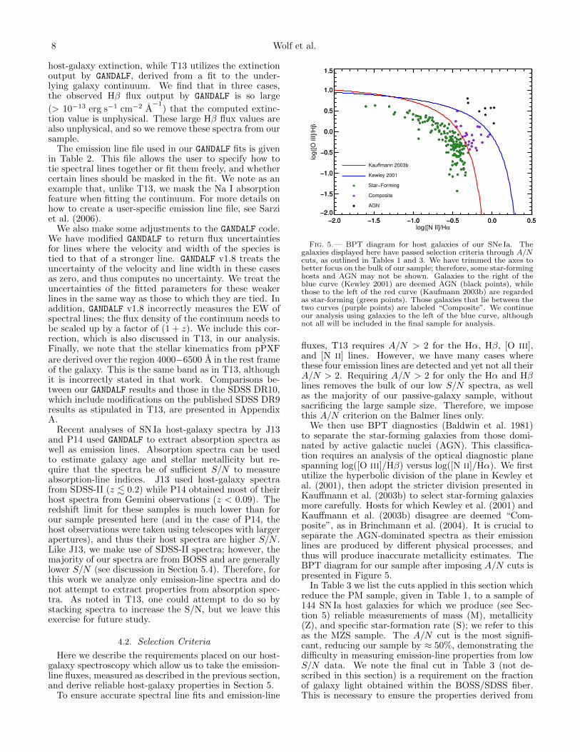
Fig. 5.— BPT diagram for host galaxies of our SNe Ia. Thegalaxies displayed here have passed selection criteria through A/Ncuts, as outlined in Tables 1 and 3. We have trimmed the axes tobetter focus on the bulk of our sample; therefore, some star-forminghosts and AGN may not be shown. Galaxies to the right of theblue curve (Kewley 2001) are deemed AGN (black points), whilethose to the left of the red curve (Kaufmann 2003b) are regardedas star-forming (green points). Those galaxies that lie between thetwo curves (purple points) are labeled “Composite”. We continueour analysis using galaxies to the left of the blue curve, althoughnot all will be included in the final sample for analysis.

fluxes, T13 requires A/N > 2 for the Hα, Hβ, [O III],and [N II] lines. However, we have many cases wherethese four emission lines are detected and yet not all theirA/N > 2. Requiring A/N > 2 for only the Hα and Hβlines removes the bulk of our low S/N spectra, as wellas the majority of our passive-galaxy sample, withoutsacrificing the large sample size. Therefore, we imposethis A/N criterion on the Balmer lines only.

We then use BPT diagnostics (Baldwin et al. 1981)to separate the star-forming galaxies from those domi-nated by active galactic nuclei (AGN). This classifica-tion requires an analysis of the optical diagnostic planespanning log([O III]/Hβ) versus log([N II]/Hα). We firstutilize the hyperbolic division of the plane in Kewley etal. (2001), then adopt the stricter division presented inKauffmann et al. (2003b) to select star-forming galaxiesmore carefully. Hosts for which Kewley et al. (2001) andKauffmann et al. (2003b) disagree are deemed “Com-posite”, as in Brinchmann et al. (2004). It is crucial toseparate the AGN-dominated spectra as their emissionlines are produced by different physical processes, andthus will produce inaccurate metallicity estimates. TheBPT diagram for our sample after imposing A/N cuts ispresented in Figure 5.

In Table 3 we list the cuts applied in this section whichreduce the PM sample, given in Table 1, to a sample of144 SN Ia host galaxies for which we produce (see Sec-tion 5) reliable measurements of mass (M), metallicity(Z), and specific star-formation rate (S); we refer to thisas the MZS sample. The A/N cut is the most signifi-cant, reducing our sample by ≈ 50%, demonstrating thedifficulty in measuring emission-line properties from lowS/N data. We note the final cut in Table 3 (not de-scribed in this section) is a requirement on the fractionof galaxy light obtained within the BOSS/SDSS fiber.This is necessary to ensure the properties derived from

9

TABLE 2GANDALF Emission-Line Setup File

Line Index Line Name Rest Wavelength Action1 L-kind2 A i3 V g/i4 sig g/i5 Fit-Kind6

(A)

0 He II 3203.15 m l 1.000 0 10 f1 [Ne V] 3345.81 m l 1.000 0 10 f2 [Ne V] 3425.81 m l 1.000 0 10 f3 [O II] 3726.03 m l 1.000 0 10 t254 [O II] 3728.73 m l 1.000 0 10 t255 [Ne III] 3868.69 m l 1.000 0 10 f6 [Ne III] 3967.40 m l 1.000 0 10 f7 H5 3889.05 m l 1.000 0 10 f8 Hε 3970.07 m l 1.000 0 10 f9 Hδ 4101.73 m l 1.000 0 10 t2410 Hγ 4340.46 m l 1.000 0 10 t2411 [O III] 4363.15 m l 1.000 0 10 f12 He II 4685.74 m l 1.000 0 10 f13 [Ar IV] 4711.30 m l 1.000 0 10 f14 [Ar IV] 4740.10 m l 1.000 0 10 f15 Hβ 4861.32 m l 1.000 0 10 t2416 [O III] 4958.83 m l 1.000 0 10 t2517 [O III] 5006.77 m l 1.000 0 10 t2518 [N I] 5197.90 m l 1.000 0 10 f19 [N I] 5200.39 m l 1.000 0 10 f20 He I 5875.60 m l 1.000 0 10 f21 [O I] 6300.20 m l 1.000 0 10 f22 [O I] 6363.67 m l 1.000 0 10 f23 [N II] 6547.96 m l 1.000 0 10 t2524 Hα 6562.80 m l 1.000 0 10 f25 [N II] 6583.34 m l 1.000 0 10 f26 [S II] 6716.31 m l 1.000 0 10 t2527 [S II] 6730.68 m l 1.000 0 10 t2590 sky 5577.00 m l 1.000 0 10 f91 sky 6300.00 m l 1.000 0 10 f92 sky 6363.00 m l 1.000 0 10 f100 Na I 5890.00 m l -1.000 0 10 t101101 Na I 5896.00 m l -1.000 0 10 f

1 The “action” sets whether each of the listed lines should be fit (f), ignored (i), orwhether the surrounding spectral region should be masked (m). As GANDALF runs, the “action” is changed by thecode; e.g., if the “action” is set to ‘m’, the line will be masked when fitting for the continuum, then changed to ‘f’when fitting for the emission lines. The subsequent fields in the setup file are only used when the “action” is setto ‘f’.2 The line-kind “l-kind” allows GANDALF to identify whether or not a line should be treated as belonging to a doubletor multiplet. All lines can be treated individually (l) or can be tied to the strongest element of their multiplet(dXX), where XX is the line index. If a line is identified as part of a doublet or multiplet, its amplitude is fixedto that of the strongest element via A i.3 Used to set the relative emission (A i > 0) or absorption (A i < 0) strength of lines in a multiplet. If a line isto be treated individually, A i is set to unity.4 Initial estimate for line velocity, km s−1.5 Initial estimate for line velocity dispersion, km s−1.6 Indicates if the position and width of the line is found freely (f) or tied (tXX) to another line, where XX is theline index.

our spectra are global host-galaxy properties. As thiscut is not based on the spectroscopy itself, but rather onhost-galaxy photometry, it is detailed in Section 5.4.

5. DERIVED HOST GALAXY PROPERTIES

In this section we describe the methods used to derivethe host-galaxy properties, both spectroscopic and pho-tometric, used in this analysis. Sections 5.1 and 5.2 de-tail the processes for computing, respectively, gas-phasemetallicities and star-formation rates from the measure-ments obtained in Section 4. In Section 5.3 we describethe source for our host-galaxy masses. We discuss fiberaperture effects – what biases may be present, how wecorrect for them, and their impact on sample selection –in Section 5.4.

5.1. Metallicity

There are several methods for estimating gas-phasemetallicity (Z ≡ log(O/H) + 12) from emission-linefluxes. Although the metallicities from each method donot have the same absolute values, relative values tend toremain consistent (i.e., a galaxy with low metallicity inone method will have low metallicity in another). Kew-ley & Ellison (2008, hereafter KE08) summarize thesetechniques and derive conversions from one metallicitycalibration into another. In this analysis we adopt thecalibration of Kewley & Dopita (2002, hereafter KD02),as recommended by (and updated in) KE08.

The KD02 algorithm is split into upper (high Z) andlower (low Z) branches based on the ratio of the [N II]and [O II] line fluxes obtained from the galaxy spectrum([O II] = [O II λ3727] + [O II λ3729]; [N II] = [N II

λ6584]). For galaxies with log([N II]/[O II]) > −1.2, the

10 Wolf et al.

TABLE 3Cumulative MZS Sample Definition

Selection Requirements Removed Total Phot-Ia Spec-IaSNe Ia

PM Sample – 345 176 169aObserved Hβ flux < 104 3 342 176 166Hα and Hβ A/N > 2 149 184 88 96Star-forming or “Composite” host 9 175 80 950.2 ≤ g-band fiber fraction < 1 31 144 78 66

a Flux density in units of 10−17 erg s−1 cm−2 A−1

metallicity is found via the real roots of the polynomial

log([N II]/[O II]) = 1106.8660− 532.15451Z

+ 96.373260Z2 − 7.8106123Z3 + 0.2392847Z4 (2)

The systematic accuracy of this method on the high-Zbranch, as stated in KE08, is ∼ 0.1 dex.

For galaxies with log([N II]/[O II]) < −1.2, the KD02method derives metallicities using an average of twodistinct R23 calibrations (for a more complete discus-sion of R23 see KE08) with a systematic uncertainty of∼ 0.15 dex. The first method utilizes the iterative proce-dure of Kobulnicky & Kewley (2004, hereafter KK04) inthe lower R23 branch, while the second (McGaugh 1991)is based on the photoionization code CLOUDY (Ferland etal. 1998) with associated analytic solutions from Kobul-nicky et al. (1999). We require that a solution is foundusing both techniques to determine an accurate metal-licity.

5.2. Star-Formation Rate

The Hα line flux is used to determine the star-formation rate (SFR) of our host galaxies, as it tracesluminosity from young (∼ 106 yrs), massive (M > 10M)stars (Kennicutt 1998). It also allows for a direct cou-pling of nebular emission to instantaneous SFR, indepen-dent of any previous star-formation history. As outlinedin Kennicutt (1998), the star-formation rate for a galaxywith a Salpeter IMF can be found by

SFR (M yr−1) = 7.9× 10−42L(Hα) (erg s−1) (3)

where the Hα luminosity is determined using the lineflux and the assumed B14 cosmology. Brinchmann et al.(2004) have shown that the conversion factor betweenL(Hα) and SFR is dependent on the mass and metallicityof the galaxy. To account for this variation, as in D11,we assume a systematic uncertainty in log(SFR) of 0.2.

We note that we correct our SFR values for apertureeffects (see Section 5.4). In addition, we compute the spe-cific star-formation rate (sSFR) by dividing the SFR bythe photometrically-derived galaxy stellar mass, which isdescribed in the following subsection.

To test the validity of our methods, we compare ourmetallicity and sSFR measurements to those reported inD11, as they also extract emission-line fluxes from BOSSand SDSS host-galaxy spectra and also compute metal-licity using the KD02 algorithm. We find that for the 39hosts which overlap in the two samples, we recover thegas-phase metallicity and SFR measurements reportedin D11. The distribution of the difference between ourmeasurements and those of D11 shows no bias and has an

approximately Gaussian distribution; 95% of the sampleagrees to within 2σ.

5.3. Host Mass

Stellar masses for our host galaxies are taken from S14and were computed using the method of Gupta et al.(2011). This method employs model spectral energy dis-tributions (SEDs) generated on a fixed grid using theFlexible Stellar Population Synthesis code (FSPS; Con-roy et al. 2009; Conroy & Gunn 2010). Synthetic pho-tometry computed from these model SEDs in the SDSSugriz bands were compared to SDSS photometry of ourhost galaxies14 while fixing the redshift to the spectro-scopic value. For more details on the FSPS model pa-rameters used and on the exact method of estimatingstellar mass, see Gupta et al. (2011). Systematic un-certainties in stellar mass estimates for normal galaxiesare generally < 0.2 dex (Conroy 2013). At best it is 0.1dex (25%), and so we incorporate this 0.1 dex into oursystematic uncertainty.

5.4. Aperture Effects

As we are deriving some galaxy properties from fixed-aperture spectra, we require a parameter that indicatesthe degree to which each spectrum is representative of aglobal average. To do this we compute in ugriz for eachspectrum the ratio of flux observed within the fiber (thefiberMag) to the total flux of the target galaxy basedon a profile fit (the modelMag). The fiber and modelmagnitudes are taken from the SDSS Catalog ArchiveServer. We refer to the derived ratio in each band as thefiber fraction. Because our sample consists of spectrafrom both 2′′ and 3′′ diameter fibers, we compute fiberfractions for both cases.

Based on the g-band fiber fraction, we remove the star-forming and “Composite” spectra whose properties areare not indicative of the global average of the targetgalaxy. First, we find that some hosts have a g-bandfiber fraction greater than one. Although objects are de-blended before the modelMag is computed, this is not thecase for the fiberMag; thus, we obtain fiber fractions > 1.After visual inspection of these cases, we conclude thatthese hosts have bright, nearby neighbors that contributeto the observed fiber magnitude. Since these spectra in-clude contamination from a galaxy other than the target,the derived properties cannot be assumed to be represen-tative of the SN Ia host. Second, all hosts with a g-bandfiber fraction < 0.2 are removed from our sample. At

14 Obtained from the DR8 Catalog Archive Server (CAS) athttp://skyservice.pha.jhu.edu/casjobs/

11

0.0 0.2 0.4 0.6 0.8 1.0

8.0

8.5

9.0

9.5

0.0 0.2 0.4 0.6 0.8 1.0g-band Fiber Fraction

8.0

8.5

9.0

9.51

2+

log[O

/H]

BOSS (2")

SDSS (3")

Total Bins

Fig. 6.— Host metallicity as a function of g-band fiber fraction forhosts that satisfy BPT cuts. The dashed line at g-band fiber frac-tion = 0.2 represents the threshold fiber fraction above which thederived gas-phase metallicity is considered indicative of the globalaverage (Kewley et al. 2005). Inverse-variance weighted binned av-erages, of approximately equal-sized bins, are plotted in red. Thereis a slight (0.07 dex) decrease in metallicity with increasing fiberfraction.

these low fiber fractions too little of the galaxy is beingmeasured to compute a global, rather than core, metal-licity (Kewley et al. 2005). These two aperture cuts, asmentioned in Section 4.2, finalize our MZS sample at 144galaxies (Table 3).

Figure 6 shows the derived host gas-phase metallicitiesas a function of g-band fiber fraction, with the dashedline indicating the lower-limit for inclusion in the MZSsample. We compute inverse-variance weighted averagesover three bins of g-band fiber fraction (such that the binsare approximately equally sized), and find little correla-tion between g-band fiber fraction and gas-phase metal-licity. This indicates that our use of different physicalscales does not have a significant effect on our metallic-ity, and thus we make no aperture-based corrections.

We also use the u-band fiber fraction to adjust our es-timate of the SFR based on the measured Hα line flux(Gilbank et al. 2010). Because our emission-line fluxmeasurements are affected by the fixed aperture size, theHα flux we measure is not a global representation of theentire galaxy. Therefore, to obtain a more reasonableestimate of the total SFR for the host, the Hα flux mea-surement is corrected by dividing by the u-band fiberfraction as in Gilbank et al. (2010) (see Appendix A).

Another important aperture effect to consider is thatour analysis uses both SDSS and BOSS spectra, with 3′′

and 2′′ fiber diameters respectively. For 19 of our SNe Ia,the hosts were targeted by both SDSS and BOSS; weuse spectra from these observations to compare the de-rived metallicities. We find the difference between themetallicity measurements to be within 0.1 dex (equiva-lent to systematic uncertainties) for 83% of hosts, ap-proximately Gaussian, and centered at zero. This indi-cates that our sample suffers no metallicity bias due toaperture effects.

The majority of the host-galaxy spectra we use wereobtained from BOSS rather than from SDSS-I/II. Pri-ority for BOSS targets was given to galaxies with a 3′′

r-band fiber magnitude < 21.25, though some galaxies

20

40

Ga

laxy C

ou

nt

BOSS

SDSS

8.2 8.6 9.0 9.412+log(O/H)

0.0

0.2

0.4

0.6

0.8

1.0

Cu

mu

lative

Fra

ctio

n

Fig. 7.— The distribution of host gas-phase metallicities forSDSS (green) and BOSS (blue) galaxies in our MZS sample, withtotal number counts shown in the top panel and the correspondingcumulative distribution function in the bottom panel. To focuson the bulk of our sample, we leave out one host with Z < 8.2from this figure. The vertical dashed line at 12+log(O/H) = 8.69represents the solar metallicity value, shown for comparison. TheSDSS spectra are systematically higher metallicity than the BOSSspectra due to how targets were selected for the two samples.

fainter than this limit were observed (Olmstead et al.2014). By contrast, SDSS-I/II spectra were obtainedfrom the SDSS Legacy Survey and other targeted sur-veys within SDSS, many of which had much brighterlimiting magnitudes. As a result, the SDSS spectratend to have higher signal-to-noise ratio and their cor-responding galaxies are at lower redshift. In addition,since they are the brightest galaxies at a given redshift,they are generally more massive and more metal-rich.This effect is displayed Figure 7. The BOSS spectrapeak at slightly lower metallicity compared to the SDSSspectra while also extending much farther into the low-metallicity regime. The median metallicity for the BOSSspectra is Z = 8.85, while the median metallicity for theSDSS spectra is Z = 8.97. It is important to rememberthat this offset is an effect of target selection, not a biasdue to the fiber aperture size, as we have demonstratedfrom hosts present in both spectroscopic samples.

Where spectra exist for both BOSS and SDSS galax-ies, we choose to use the SDSS spectrum for our analysesin Section 6. In addition to being higher S/N spectraon average, all SDSS spectra targeted the core of thegalaxy, while some spectra from the BOSS ancillary pro-gram targeted the location of the SN itself (Olmstead etal. 2014). In all cases where only BOSS spectra exist fora galaxy, the fiber was centered on the galaxy core. To-gether with the cuts in this section and examination ofpotential sources for aperture bias, this selection createsa consistent, high-quality set of data for our analyses.

6. RESULTS

In Table 7, we present our derived SN Ia and host-galaxy properties for all data used in this analysis. All345 of these SNe Ia have passed SN light-curve qualitycuts, have an identified host-galaxy spectrum, and have aphotometrically-derived host mass (the PM sample; Ta-ble 1). For a subset of 144 of these SNe Ia, the MZS

12 Wolf et al.

sample, we have spectroscopically measured global host-galaxy metallicities and star-formation rates. Table 3summarizes the requirements placed on this sample. Thefull version of Table 7 is available in the electronic versionof this work.

The derived host-property uncertainties quoted in Ta-ble 7 do not include any systematic uncertainties previ-ously discussed (0.1 dex, 0.2 dex, and 0.1 dex for metal-licity, SFR, and stellar mass, respectively). Similarly,error bars in subsequent plots (e.g. Figures 11 and 12)reflect only statistical uncertainties for clarity. However,when fitting for linear trends, systematic uncertaintiesare added in quadrature to the quoted statistical uncer-tainties. As S14 reports asymmetric mass uncertainties,we choose the larger value as the single, conservative es-timate.

In the following analysis, we discuss our derived hostproperties and SN Ia properties, as well as explore corre-lations between them. We use the IDL LINMIX routine,which employs the linear regression model presented inKelly (2007), to assess the strength of observed correla-tions:

y = mx+ b+ ε (4)

Here, m is the fit slope, b is the fit intercept, and ε is thescatter about the best-fit regression line. As described inKelly (2007), we assume ε is drawn from a normal dis-tribution with mean zero and variance σ2. Throughoutthis work we report the intrinsic dispersion (σ) and itsuncertainty, computed by taking the square root of theposterior distribution of the best-fit variance. We definethe significance of a non-zero slope as m/σm, where mis best-fit slope and σm is the error on the slope. LIN-MIX allows for uncertainties in the dependent and inde-pendent variables (assuming Gaussianity) and employsa Bayesian approach using Markov Chain Monte Carlo(MCMC). Posterior distributions for at least 10,000 iter-ations of the MCMC are used to determine the regressioncoefficients and their errors. For completeness, we reportthe median and standard deviation of the posterior dis-tributions of the best-fit slope, intercept, and dispersionin our results tables. This method of linear fitting waschosen over other linear regression techniques (such asleast-squares) as we find that the LINMIX fits providemore realistic estimates for our fit parameter errors.

We also use the Spearman rank correlation coefficientand corresponding significance test to study the relation-ship between SN Ia and host-galaxy properties. This isa nonparametric measure of statistical dependence thatrequires that the relationship between the two variablesof interest is monotonic, but not necessarily linear. Thevalue of the coefficient, ρ, ranges from −1 to +1 with|ρ| = 1 indicating a perfectly monotone relation. Thenull hypothesis for this test states that there is no corre-lation between the dependent and independent variable;the associated p-value describes the chance that randomsampling of the data would have generated the observedcorrelation. While this technique provides important in-sight into our SN Ia-host-galaxy correlations, we mustbe cautious as it does not account for large differencesin the measurement errors of different data points whencomputing the correlation coefficient.

A general outline is as follows: Section 6.1 describesour derived host-galaxy properties. Section 6.2 discusses

020

40

60

80

100

120

140

PM

Sa

mp

le

Phot−Ia

Spec−Ia

0.0 0.1 0.2 0.30.0Redshift

010

20

30

40

50

60

MZ

S S

am

ple

Phot−Ia

Spec−Ia

Fig. 8.— Redshift distributions of the PM and MZS samples.Histograms are stacked such that the number of Spec-Ia (green)and Phot-Ia (blue) shown in each bin add to the total number ofSNe Ia in that bin. The mean and median redshifts of the PM andMZS samples are each z = 0.24. For both samples, the medianredshift of the Spec-Ia is 0.19 and the median redshift of the Phot-Ia is 0.26.

the stretch and color of our SNe Ia and correlations be-tween these parameters and host-galaxy properties. Sec-tion 6.3 examines the individual relations between HRand host-galaxy mass, gas-phase metallicity, and specificstar-formation rate, separately. In Section 6.4 we explorethe interplay between these host properties and how theyaffect trends with HR when fit simultaneously.

6.1. Host-Galaxy Properties

The redshift distributions of the PM and MZS hostsare shown in Figure 8. The mean and median redshiftsfor both the PM and MZS samples is z = 0.24, andthe shapes of the redshift distributions are consistent.The median redshifts of the Spec-Ia and Phot-Ia in sub-samples are 0.19 and 0.26, respectively, in both the PMand MZS. We thus conclude that the requirements weimpose on our host-galaxy spectroscopic data when cre-ating the MZS sample does not result in any redshift biasrelative to the PM sample.

We present in Figure 9 the host-galaxy stellar massdistribution for both our PM and MZS samples, both asa whole and as a function of redshift. While the MZShost-galaxy sample only contains star-forming galaxiesthrough the requirement of measurable emission lines,the PM sample consists of both star-forming and ellip-tical galaxies. The inclusion of elliptical galaxies, whichhave a higher mass on average, results in the PM samplespanning a slightly larger range in masses with a highermean mass (log(M/M)= 10.5) than the MZS sample(log(M/M)= 10.2). We also see in the right panels ofFigure 9 that there is no noticeable trend of host masswith redshift for our sample over this redshift range, in-dicating that our sample has no strong differential biaswith redshift.

In Figure 10 we show the distributions of metallicityand specific star-formation rates from our MZS sam-ple. The mean gas-phase metallicity for our sample isZ = 8.84, and the mean sSFR is log(sSFR)= −9.43.While the sSFR distribution is roughly Gaussian, the

13

20

40

60N

um

be

r of

Hosts

PM

MZS

8 9 10 11 12log(M/M

O •)

0.0

0.2

0.4

0.6

0.8

1.0

Cu

mu

lative

Fra

ctio

n

log(M

/MO • )

8.5

9.5

10.5

11.5

PM

0.05 0.10 0.15 0.20 0.25 0.30 0.35Redshift

log(M

/MO • )

8.5

9.5

10.5

11.5

MZS

Fig. 9.— Mass distributions of our PM (dashed) and MZS (solid) galaxies are displayed in the top left panel. The mean of the PM andMZS mass distributions (in log(M/M) are 10.5 and 10.2, respectively. The bottom left panel presents the cumulative fraction of hosts asa function of mass. The right panels show our galaxy masses as a function of redshift.

metallicity distribution is negatively skewed, althoughthere are few galaxies with sub-solar metallicities evenin the long low-metallicity tail. As shown in the insetpanels in Figure 10, we see no evolution of metallicity orsSFR with redshift.

As we use different IMFs, methods, selection criteria,and calibration techniques, we cannot directly compareour results to previous studies. However, we can quali-tatively assess how our host-property distributions com-pare to those of other surveys. The peak host-galaxymass in the PM sample is consistent with that in the PTF(P14), SNFactory (C13), SNLS (Sullivan et al. 2010), andPan-STARRS1 (PS1; Scolnic et al. 2014b).

We notice our host-galaxy mass distribution containsrelatively fewer galaxies with log(M/M) . 9.0. Weattribute this primarily to the BOSS targeting criteriaand the use of the SDSS DR8 catalog for host identifica-tion. Given that our Phot-Ia sample depends on redshiftsfrom BOSS, which only targeted hosts brighter than acertain magnitude, we expect this sample to be biasedagainst SNe in low-luminosity (low-mass) hosts. We alsolose low-mass hosts due to the r-band magnitude limitof 22.2 for SDSS DR8, which is the catalog used to selecthost galaxies in S14.15 In addition, our choice of mass-fitting technique may also contribute to the dearth oflow-mass hosts. We use FSPS masses in this work whichare shown in Figure 23 of S14 to be ≈ 0.3 dex higher thanthe masses derived from ZPEG (a code commonly usedby other works). Therefore, we note that our reducedhost-mass range may affect our derived trends with HR(Section 6.3).

In the MZS sample, the derived metallicities of P14 forPTF host galaxies are biased substantially lower than

15 Though a deep co-added image catalog exists for SDSS Stripe82 (Annis et al. 2014), these images contain SN light for SNe oc-curring in 2005. Ideally, SN surveys in the future should createcustom co-added images excluding images with SNe and use thesefor host identification and host-galaxy studies.

our metallicities, but as the typical offset between thecalibration used by us and in that work is 0.2-0.3 dex,the range of measured values are consistent. C13 uses acalibration that typically returns a wider range of metal-licities, and this is seen in their results compared to thiswork. However, although C13 also finds the peak of theirdistribution at 12+log(O/H)≈ 9.0, they have a greaterfraction of their host-galaxies at sub-solar than can beexplained through calibration techniques alone. In ad-dition, we find that the sSFR distribution of the MZSsample also exhibits a lack of low-sSFR hosts when com-pared to other studies. One reason for this differenceis that some studies (Sullivan et al. 2010; Childress etal. 2013) with hosts with lower star-formation rates relyon host photometry, rather than spectroscopy, to obtainSFR measurements and are thus not limited by spectralquality requirements.

The differences in these property distributions likelystem from our spectral quality requirements. We im-pose a cut on the A/N of the Hα and Hβ lines to ensuregood spectral quality, but by doing so reject those spectrawith lower emission-line flux measurements. If we removethis A/N criterion, an additional 41 hosts would be in-cluded in the MZS sample. Of these 41, 26.8% have sub-solar metallicity. Additionally, we find that 58.5% of the41 additional hosts have low sSFR (log(sSFR) < −10).Adding these hosts into our sample would not signifi-cantly impact the fraction of low-metallicity hosts, butwould raise the fraction of low-sSFR hosts from 9.7% to20.5%. However, we believe the quality of these spectrais not sufficient to produce reliable host-property esti-mates, and so we do not include these in our sample.

6.2. SN Ia Light-Curve Properties

SN Ia light-curve parameters such as color (c) andstretch (x1) – the essential calibration tools for usingSNe Ia as distance indicators – have long been knownto correlate with host environment (Hamuy et al. 1996;

14 Wolf et al.

7.8 8.0 8.2 8.4 8.6 8.8 9.0 9.212+log(O/H)

0

10

20

30

Nu

mb

er

of

Ho

sts

0.05 0.15 0.25Redshift

8.6

8.8

9.0

9.2

9.41

2+

log

(O/H

)

-12 -11 -10 -9 -8log(sSFR)

0

10

20

30

Nu

mb

er

of

Ho

sts

0.05 0.15 0.25Redshift

-11

-10

-9

-8

log(s

SF

R)

Fig. 10.— The left panel shows the metallicity distribution ofgalaxies in our MZS sample. The mean of the metallicity distribu-tion is Z = 8.84. The right panel shows the sSFR distribution ofgalaxies in our MZS sample. The mean of the sSFR distributionis log(sSFR)= −9.43. The inset figures of both panels display therespective host properties as a function of redshift. Axes of theinset figures have been adjusted to focus on the metallicity andsSFR redshift dependence; as such, some data points are excludedfrom the plots.

Gallagher et al. 2005). Figure 11 shows the SN Ia stretchand color as a function of our derived host-galaxy prop-erties. We observe the correlations seen by Howell et al.(2009) and Sullivan et al. (2010): more massive galax-ies host fainter, redder SNe Ia. We also find that SNe Iawith higher c occur in galaxies with lower specific star-formation rates. Since the SN Ia color parameter con-tains information not just on the intrinsic color of theSN but also effects of host-galaxy dust extinction, it isexpected that both massive galaxies and those with lowspecific-star formation should host redder SNe Ia. It isinteresting to note that we find low-metallicity galax-ies tend to host only blue SNe Ia, to an extent not seenin low-mass or high-sSFR galaxies (properties that arecorrelated with low metallicity). This metallicity-colorrelation is consistent with what is found in C13 and P14.

To quantify the strengths of these correlations, weperform a Spearman rank test on each combination ofSN Ia and host property displayed in Figure 11. In each

of the six cases, the correlation coefficient is non-zero;however, only the SN Ia stretch-host mass correlationexhibits enough evidence to reject the null hypothesis(ρ = −0.308, p = 5.305× 10−9).

6.3. HR as a Function of Host-Galaxy Properties

We now examine whether the stretch- and color-corrected luminosities of SNe Ia (and thus HRs) showcorrelations with properties of their host galaxies. Linearfits to the data using the LINMIX routine are shown onthe figures included in this section and the correspondingresults are reported in Table 4. Spearman rank correla-tion statistics for each linear fit are also presented inTable 4. We note that the posterior distributions of themodel parameters of these fits are roughly Gaussian. Todetermine the model parameters of these fits, we choosethe point estimator to be the median of the posteriordistribution, limiting the effects of outliers in the distri-bution. Errors on the fit parameters are obtained usingthe standard deviation of the respective posterior distri-bution. Host-galaxy properties are also split to createlow and high mass (metallicity, sSFR) bins which arethen used to compute the difference between the HR inthese bins (“HR step”). The split point of each propertyis chosen to be the median of its respective distribution,thus creating two bins of equal number. We define the“HR step” as the difference between the high and low-binned inverse-variance weighted averages. When com-puting the significance of the step (the mean and uncer-tainties on the mean), we fit for the unknown intrinsicscatter that ensures χ2/DoF ≈ 1 after the step is re-moved. These bins are also included in relevant figuresin this section. We note that when we refer to the overor under-luminosity of SNe Ia in this section, this refersto the luminosity after light-curve corrections have beenapplied.

Figure 12 shows HR as a function of mass for the PMsample. Using LINMIX, a non-zero slope of the linearfit is detected at 3.6σ. We also take the difference be-tween the inverse-variance weighted averages of the highand low-mass bins and measure the “HR step” to be−0.048 ± 0.019 magnitudes. A similar trend is presentin the MZS sample; the best-fit slope and the HR stepare both shown to be consistent within 1σ that of the fullPM sample. Our results show that more massive galaxieshost over-luminous SNe Ia, supporting previous findings(Lampeitl et al. 2010; Sullivan et al. 2010; Gupta et al.2011; Childress et al. 2013; Betoule et al. 2014).

The results of the Spearman rank correlation test forboth the PM and MZS samples further support the sig-nificance of the HR-mass relation. In both cases, wefind ρ ≈ −0.2, which indicates that more massive galax-ies host overluminous SN Ia. For both samples, thereis a less than 2% chance that this correlation is due tochance, and thus we again conclude that this correlationis significant.

Several recent studies suggest that HR as a functionof host-galaxy mass resembles a smoothly-varying stepfunction rather than a line. To explore this idea of a“mass step”, we fit an empirical continuous step functionto our data in the PM sample. We choose a function ofthe form

HR = A

(2

1 + e−B(x−C)− 1

)(5)

15

-2

-1

0

1

2

3

-2

-1

0

1

2

3S

ALT

2 x

1

8 9 10 11log(M/M

O •)

-0.2

0.0

0.2

0.4

SA

LT

2 c

-12 -11 -10 -9log(sSFR)

8.0 8.5 9.0 9.512+log(O/H)

Fig. 11.— SNe Ia color (c) and stretch (x1) as a function of derived host properties. The left panel displays data from the PM sample;the middle and right panels show data from the MZS sample. Axes have been truncated to focus on the bulk of the data.

TABLE 4LINMIX Linear Fit Results for HR as a Function of Derived Host-Galaxy Properties

Host Sample Na Splitb HR Step Slope Intercept σ Sigc ρ p-valueProperty Value [mag] [mag]

Mass PM 345 10.5 0.048 ± 0.019 −0.055 ± 0.015 0.570 ± 0.160 0.121 ± 0.009 3.62σ −0.1708 0.0015Mass MZS 144 10.2 0.082 ± 0.030 −0.071 ± 0.029 0.728 ± 0.293 0.136 ± 0.014 2.46σ −0.2094 0.011812+log(O/H) MZS 144 8.9 0.057 ± 0.031 −0.579 ± 0.409 5.162 ± 3.641 0.125 ± 0.021 1.42σ −0.1811 0.0299sSFR MZS 144 −9.4 0.013 ± 0.031 0.019 ± 0.046 0.190 ± 0.437 0.140 ± 0.014 0.42σ 0.0965 0.2500

aSample size.

bValue used to create high and low-mass (metallicity, sSFR) bins of equal number. The median of the respective host-property distribution.

cSignificance of a non-zero slope.

8 9 10 11 12 13

−1.0

−0.5

0.0

0.5

1.0

8 9 10 11 12 13log(M/M

O ·)

−1.0

−0.5

0.0

0.5

1.0

µS

N−

µz

Fig. 12.— HR as a function of host-galaxy mass for the PMsample. The LINMIX linear fits to the data are shown in dashedblack; red squares represent inverse-variance weighted binned av-erages, with bins split at log(M/M)= 10.5. The significance of anon-zero slope is 3.6σ and the difference in HR between the highand low-mass bins is 0.048 magnitudes. This result indicates thatmore massive galaxies host over-luminous SNe Ia.

where the parameter A controls the amplitude, B con-trols the steepness of the step, and C indicates thestep position. The independent variable, x, is the hostmass, log(M/M). We use the IDL routine MPFIT-FUN (Markwardt 2009) to perform a least-squares fit,using input parameters motivated by results in previousworks and find that the resulting best-fit to the data ishighly sensitive to the choice of input parameters. Wealso compute the best-fit to inverse-variance weighted av-erage bins of varying bin width and minimum number ofSNe Ia per bin and find that choice of bin width andnumber of SNe Ia per bin significantly affects the best-fitresults.

Therefore, we choose to explore the shape of the HR-mass relation using nonparametric regression. We em-ploy the loess routine in the R statistical software pack-age, based on cloess of Cleveland et al. (1992). Thismethod of locally-weighted smoothing combines linearregression in a k-nearest-neighbor based model and relieson a user-input bandwidth, also known as the span (α),to determine the proportion of the data to be used in eachlocal regression (i.e., a fit at some point x is computedusing its neighbors and contributions from neighboringpoints are weighted based on their distance from x).

16 Wolf et al.

8.5 9.0 9.5 10.0 10.5 11.0 11.5 12.0

−0.3

−0.2

−0.1

−0.0

0.1

0.2

0.3

8.5 9.0 9.5 10.0 10.5 11.0 11.5 12.0log(M/M

O ·)

−0.3

−0.2

−0.1

−0.0

0.1

0.2

0.3

µS

N−

µz

Fig. 13.— Non-parametric regression fit of HR as a function ofhost-galaxy mass. The best-fit is presented in red with the approx-imate corresponding 1σ confidence interval. A span of α = 0.6 wasused for the fit.

While this method cannot produce an empirical model,it does illustrate the general shape of the data.

The results of the loess regression are presented inFigure 13, with the HR axis truncated to better focus onthe fit. The best-fit to the data is shown in red with anapproximate corresponding 1σ confidence interval. Thismethod of local regression is sensitive to edge effects,but has no consequence on the resulting best-fit for thebulk of the data. Therefore, the behavior of the best-fitat the low and high-mass extremes must be interpretedwith caution. After testing multiple spans, we determinea span that responds best to fluctuations in the data ofα = 0.6.

As shown in Figure 13, there appears to be a rela-tively smooth transition region in the HR-mass relationbetween 10.0 . log(M/M) . 10.4. However, becauseof the sensitivity of the fit at the edges, the shape ofthe “step regions” is not well represented. In addition,the computation of the best-fit did not include measure-ment error, which may affect the observed behavior. Theshape of the HR-mass relation is similar to the behaviorreported in C13 and J13; the slope of the transition re-gion in J13, C13, and this work is roughly −0.2. Wenote that our results should be correlated with what ispresented in J13 and C13 as their analyses utilize a sub-set of the SDSS SNe Ia. Despite the shortcomings of ourchosen fitting technique, the nonparametric fit is an in-teresting interpretation of the HR-mass relation and amore rigorous treatment should be considered for futurestudies.

We next examine the correlation between HR and host-galaxy gas-phase metallicity; the results are shown inFigure 14. The best-fit linear relation has a negativeslope with 1.4σ significance, suggesting that more metal-rich galaxies host more over-luminous SNe Ia. Examiningthe difference between our low and high-metallicity binsreveals an “HR Step” of 0.057 magnitudes with 1.86σ sig-nificance. When analyzing this relation using the Spear-man coefficient, we find a statistically significant cor-relation (ρ = −0.1811, p = 0.0299) between HR andgas-phase metallicity. Although the LINMIX results donot recover a significant correlation, the other statistical

8.0 8.2 8.4 8.6 8.8 9.0 9.2 9.4

−1.0

−0.5

0.0

0.5

1.0

8.0 8.2 8.4 8.6 8.8 9.0 9.2 9.412+log(O/H)

−1.0

−0.5

0.0

0.5

1.0

µS

N−

µz

Fig. 14.— HR as a function of gas-phase metallicity for the MZSsample. These points are separated at 12+log(O/H) = 8.9 to createhigh and low-metallicity bins. Red squares indicate the inverse-variance weighted average of these bins. The difference betweenthe binned averages is 0.057 magnitudes. The linear LINMIX fitto the data is shown in dashed-black; there is a 1.4σ significance ofa non-zero slope which suggests that more metal-rich galaxies hostover-luminous SNe Ia.

analysis tools indicate that there is a significant differ-ence between the low and high-metallicity populations.This suggests that the behavior of HR-metallicity rela-tion may not be adequately represented by the LINMIXlinear fit.

Finally, we investigate HR as a function of sSFR. Theseresults are shown Figure 15. The significance of thistrend deviating from a non-zero slope as determined byLINMIX, however, is only 0.42σ. In addition, the differ-ence between the average HR in the high and low-sSFRbins is 0.013 magnitudes with 0.42σ significance. Thetrend seen here is the weakest correlation observed be-tween HR and host-galaxy properties. The results of theSpearman correlation test (ρ = 0.0965, p = 0.25) sug-gest that we do not have enough evidence to reject ournull hypothesis; the HR-sSFR trend resembles a randomsampling of uncorrelated variables.

As discussed in Section 6.1, our cut on the Hα andHβ A/N , which is imposed to ensure spectral quality,removes 41 hosts from the MZS sample. If we add thesehosts back into the MZS sample and recompute the slopeof the HR-sSFR relation we find a slope of 0.021± 0.02,which is within 0.1σ of the slope observed using theMZS sample. A Spearman rank test on this new sam-ple also shows little evidence of an HR-sSFR correlation(ρ = 0.1337, p = 0.0695). This indicates that the A/Nrequirement and the lack of very low-sSFR hosts doesnot have a strong effect on our trend of HR with hostsSFR.

6.4. HR as a Function of Multiple Host-GalaxyProperties Simultaneously

Our wealth of data allows not only an investigation ofHR as a function of an individual host-galaxy property,but as a function of several host properties simultane-ously. We perform linear fits of HR using combinations oftwo, and a combination of all three, derived host-galaxyparameters. For these linear fits, we include the relationwith SFR as a opposed to sSFR as the sSFR and mass

17

−12 −11 −10 −9 −8 −7

−1.0

−0.5

0.0

0.5

1.0

−12 −11 −10 −9 −8 −7log(sSFR)

−1.0

−0.5

0.0

0.5

1.0

µS

N−

µz

Fig. 15.— HR as a function of specific star-formation rate forthe MZS sample. Points are separated at log(sSFR) = −9.4 tocreate high and low-sSFR bins. Red squares indicate the inverse-variance weighted average of these bins. The difference betweenthe binned averages is 0.013 magnitudes. The linear LINMIX fitto the data is shown in dashed-black; there is a 0.42σ significanceof a non-zero slope. This slight correlation suggests that galaxieswith lower specific star formation rates host over-luminous SNe Ia.

uncertainties are correlated. We then examine the HR-metallicity and HR-sSFR relation in several mass binsand also after correcting for the HR-mass relation. Sincemass appears to have the most dominant effect on HR,removing this dependence could provide important in-sight into the degeneracy of our host-galaxy properties.

We first use the LINMIX package for multiple linearregression to determine the best-fit relation between HRand multiple host-galaxy parameters. When using allthree host properties, this function takes the form:

HR = a× log(M/M) + b× (12 + log(O/H))

+ c× log(SFR) + d+ σ2 (6)

where the coefficients a, b, c, d, and σ2 are the parametersto be fit. These same coefficients are fit using combina-tions of two host properties: i.e.,

HR = a×log(M/M)+b×(12 + log(O/H))+d+σ2 (7)

HR = a× log(M/M) + c× log(SFR) + d+ σ2 (8)

HR = b× (12 + log(O/H)) + c× log(SFR) + d+ σ2 (9)

We assume the errors on the host-parameters are uncor-related.

When fitting for Equation 6, repeated trials (i.e, run-ning LINMIX multiple times) do not yield the same fitresults. For each fit parameter, results between trialsare consistent within 1σ but can have dramatically dif-ferent values (e.g., a = −0.374 ± 31.68 compared toa = 0.53 ± 2.67). We perform 20 trials of the samelinear fit and find a substantial variance between fit-parameter outputs for each trial and strong skewness inthe fit-parameter distributions. Although repeated fit-parameter outputs are not identical, the results of eachfit are consistent with no significant correlation betweenHR and all host-galaxy properties.

In addition, we perform 20 trials of each of the fitsusing two host-galaxy properties (Equations 7-9). Fit-

parameter distributions with similar variance and skew-ness are observed using Equations 7 and 9; these fitsare also consistent with no correlation. The output fitparameters using host-galaxy mass and SFR are nearlyidentical between the different trials, and the mass com-ponent is significant at ≈ 1σ, again suggesting that thefit is consistent with no correlation.

We find that the large errors on our model parametersare due, in part, to an inappropriate choice of intervalestimator. Upon further analysis, we find that manyof the LINMIX model parameter posterior distributionsare highly non-Gaussian with strong skewness and highkurtosis. While we continue to use the median of the dis-tribution as our point estimator, we recompute a new in-terval estimator rather than use the standard deviation;we find the interval, about the median, that contains ap-proximately 68% of the distribution. We take the averageof the lower and upper bounds and use this as the un-certainty. Using this method, we obtain more reasonableerrors on our fit parameters (i.e., a = −0.374 ± 31.68becomes a = −0.374 ± 2.67). However, utilizing thisnew estimator does not generally affect the significancesof correlations observed between HR and multiple host-galaxy properties simultaneously.

We also study the dependence of HR on metallicityas well as on sSFR while imposing different criteria onhost mass to try to control for the apparently dominanteffect of mass. First, we remove the HR-mass dependenceby adding the measured PM sample “HR step” of 0.049magnitudes to the HR of our higher-mass (log(M/M) ≥10.2) MZS hosts. We then re-fit HR as a function ofmetallicity and also HR as a function of sSFR (this timeincluding measurement errors again). In both cases, thedirection of the best-fit slope is the same as that fit withthe entire MZS sample. However, the significance of non-zero slopes in both cases is < 1σ. We next investigateHR as a function of metallicity and sSFR in mass bins.Our first separation is into low and high-mass bins, splitat log(M/M) = 10.2, shown in Figure 16. In each case,the significance of a non-zero slope for the best-fit to thedata is . 0.8σ, which is consistent with flatness.

Unfortunately, each of these tests are consistent withno correlation between HR and multiple host-galaxyproperties. This is perhaps largely due to the variationin measurement errors between the properties; i.e. pho-tometric stellar masses are much easier to estimate andhave smaller uncertainties than spectroscopically-derivedproperties such as metallicity and SFR. We recommendthat future surveys interested in studying these correla-tions obtain high S/N host-galaxy spectra for as manySNe Ia host galaxies. We also recommend further inves-tigation of how to incorporate correlations, both physicaland in measurement uncertainty, between various host-galaxy properties in future studies of this type. Hope-fully, combining the results of these efforts will provide abetter understanding of the physical mechanism drivingthese observed trends.

7. DISCUSSION

In this section, we compare our linear fit results of HRas a function of host-galaxy properties to those reportedin previous studies. We also separate the PM and MZSsamples into Spec-Ia and Phot-Ia subsets to assess theeffect of including a sample of photometrically-classified

18 Wolf et al.

8.0 8.2 8.4 8.6 8.8 9.0 9.2 9.4

−1.0

−0.5

0.0

0.5

1.0log(M/M

O ·) ≤ 10.2

8.0 8.2 8.4 8.6 8.8 9.0 9.2 9.412+log(O/H)

−1.0

−0.5

0.0

0.5

1.0µ

SN−

µz

8.4 8.6 8.8 9.0 9.2 9.4

−1.0

−0.5

0.0

0.5

1.0log(M/M

O ·) > 10.2

8.4 8.6 8.8 9.0 9.2 9.412+log(O/H)

−1.0

−0.5

0.0

0.5

1.0

µS

N−

µz

−11.0 −10.5 −10.0 −9.5 −9.0 −8.5 −8.0 −7.5

−1.0

−0.5

0.0

0.5

1.0log(M/log(M/M

O ·) ≤ 10.2

−11.0 −10.5 −10.0 −9.5 −9.0 −8.5 −8.0 −7.5log(sSFR)

−1.0

−0.5

0.0

0.5

1.0

µS

N−

µz

−12 −11 −10 −9 −8

−1.0

−0.5

0.0

0.5

1.0log(M/M

O ·) > 10.2

−12 −11 −10 −9 −8log(sSFR)

−1.0

−0.5

0.0

0.5

1.0

µS

N−

µz

Fig. 16.— HR as a function of metallicity and specific star-formation rate for the MZS sample in low and high-mass bins. LINMIX linearfits to the data are shown in dashed-black. In each case, the significance of a non-zero slope is . 0.8σ.

SNe Ia on studies of HR and host properties. Finally,we discuss the differences between the star-forming andpassive galaxies in our PM sample.

7.1. Comparing with Previous Studies

We compare the correlations observed in this work be-tween HR and host-galaxy properties with those reportedin previous studies and present a sample of HR-host-galaxy correlations as well as fit significances as they arereported in the literature. In some cases, a linear best-fit to the data was not provided, and thus we providethe significance of the binned-average HR-step. Becauseof differences in metallicity calibrations and IMFs usedfor host-mass calculations, we encourage the reader touse caution when comparing linear fit results from allprevious works directly. However, we can consider thestrengths and significances of the linear correlations be-tween HR and host-galaxy properties to get a qualitativesense of how these studies compare. We present this sum-mary in Table 5 and note that the list of works includedonly represents a subset of the literature.

As seen in Table 5, the results of this study confirmmuch of what is established in the literature. In fivestudies using a sample of more than 100 SNe Ia, a sig-nificant linear correlation (& 3σ) was found suggestingmore massive galaxies host over-luminous SNe Ia; it ispossible that the three studies that did not detect such

a correlation did not have large enough samples to de-tect as strong of an effect. Although the HR step withhost-galaxy mass observed for the PM sample in thiswork is smaller than what is reported in several otherstudies, it is consistent at . 1.7σ. The trend observedbetween HR and host-galaxy gas-phase metallicity andsSFR is also consistent with existing results, particularlythat the HR-sSFR correlation is the weakest observed.

When comparing to D11, it is important to clarify thatthey computed two estimates of sSFR: “sSFRspec” (usinghost-galaxy masses determined from the spectroscopic fitto the galaxy continuum) and “sSFRphot” (using massesderived from host-galaxy photometry). In their study,they find a > 3σ correlation between HR and sSFRspec.Unfortunately, we are unable to compute spectroscopicmasses (and thus sSFRspec) in our current emission-lineanalysis and suggest this for future study. However,D11 find that the correlation between HR and sSFRphot

is only significant at the 1.2σ level.16 Given that themethod we use to compute sSFR in this work is analo-gous to D11’s sSFRphot, it is not unexpected that we seea significance of similar strength.

16 As expounded in D11, the difference between sSFRspec andsSFR phot (and thus their trends with HR) might be due to cor-rections for aperture effects which are applied to sSFRphot but notto sSFRspec. See Section 4.2 of D11 for more details.

19

TABLE 5Comparison of correlations found between HR and host galaxy mass (M), gas-phase metallicity

(Z), and specific star formation rate (S)

Paper SN Survey Host Sample HR Step Slope a Slopeb

Property Size (mag) (mag/dex) Significance (σ)

This work (PM) SDSS-SNS M 345 0.048 ± 0.019 −0.055 ± 0.015 3.6σ (L)This work (MZS) SDSS-SNS M 144 0.082 ± 0.030 −0.071 ± 0.029 2.5σ (L)Sullivan ‘10 SNLS M 195 0.080 ± 0.020 −0.042 ± 0.013 3.3σ (L)Lampeitl ‘10 SDSS (z ≤ 0.21) M 162 0.100 ± 0.025 −0.072 ± 0.018 4.9σ (L)Gupta ‘11 SDSS M 206 0.096 ± 0.028 −0.057 ± 0.019 3σ (L)Kelly ‘10 CfA3 M 62 0.094 ± 0.045 −0.150 ± 0.060 2σ (L)c

C13 SNf M 115 0.085 ± 0.028 −0.043 ± 0.014 3.1σ (L)P14 PTF M 50 0.085 ± 0.047 −0.041 ± 0.030 1.4σ (L)Scolnic ‘14 Pan-Starrs1 M 112 0.040 ± 0.032 – 1.25σ (B)This work (MZS) SDSS-SNS Z 144 0.057 ± 0.031 −0.579 ± 0.409 1.4σ (L)Konishi ‘11 SDSS Z 72 0.130 ± 0.060 – 1.8σ (B)D11 SDSS (z ≤ 0.15) Z 34 0.091 ± 0.021 – 1.3σ (L)d,e

C13 SNf Z 69 0.103 ± 0.036 −0.106 ± 0.043 2.5σ (L)P14 PTF Z 36 0.115 ± 0.046 −0.358 ± 0.176 2σ (L)This work (MZS) SDSS-SNS S 144 0.013 ± 0.031 0.019 ± 0.046 0.4σ (L)P14 PTF S 48 0.070 ± 0.041 −0.019 ± 0.077 0.25σ (L)D11 SDSS (z ≤ 0.15) Sc 34 – – 1.2σ (L)d

a Slopes presented use the sign convention where Hubble residuals are defined as HR = µSN − µz . This switches thesign of the values reported in Sullivan et al. (2010) and Lampeitl et al. (2010).b We have included significances for linear fits (L) and well as differences in high and low-mass (metallicity, sSFR) bins(B) (for those papers which do not provide linear fit results).c Result quoted is from using SALT2.d sSFRphot (see D’Andrea et al. 2011).e The uncertainty quoted on the HR Step is as reported as does not include intrinsic scatter.

7.2. Photometric vs. Spectroscopic SN Ia Subsets

Here we consider the Phot and Spec-Ia subsets of thePM and MZS samples separately and re-compute cor-relations between HR and host-galaxy properties. Fig-ure 17 displays the linear fits for the separate datasetsand the fit results are presented in Table 6. Generally,in each study of HR as a function of host property usingjust the Spec-Ia, the significance of a non-zero slope is. 2σ. The significance of a non-zero correlation betweenHR and host-galaxy mass using the Phot-Ia is 3.9σ,whilethe significance of the relation using only the Spec-Ia is1.5σ. When using the Phot-Ia MZS subsample, the sig-nificances of a non-zero HR-metallicity correlation andnon-zero HR-sSFR correlation are 1.6σ and 1.1σ, respec-tively. As evident in Figure 17, the correlation betweenHR and metallicity for the Phot-Ia may be best-fit by anon-linear function. We find that in all cases of HR as afunction of host property, the linear fits obtained for theSpec-Ia are in the same direction as those for the Phot-Ia.The slopes of the linear fits for the Phot-Ia and Spec-Iasubsamples, for the HR-metallicity and HR-sSFR rela-tions, are consistent within 1.3σ. The slopes of the fitsof the HR-mass relation between the Phot-Ia and Spec-Iasamples are consistent at 2.3σ; however, both are consis-tent with the slope recovered using the full PM samplewithin 1.5σ.

The weaker HR-mass correlation in the Spec-Ia sampleis a bit unexpected, especially when comparing to previ-ous analyses using SDSS SNe Ia. In particular, we wouldexpect a similar significance to that reported in Guptaet al. (2011), which uses a comparably-sized sample ofspectroscopically-confirmed SNe Ia, also from the SDSS-SNS. However, we note that while many of the SNe Iaused in this analysis overlap with those in the Guptaet al. (2011) sample, there are several key differences in

our sample construction, namely: sample redshift cuts,SN Ia light-curve quality criteria, requirements on host-galaxy spectroscopy, and host-galaxy photometry usedto compute stellar masses. We find that only 94 SNe Iaoverlap between the Gupta et al. (2011) sample and ourPM sample. A comparison of the median of the best-fit LINMIX posterior slopes of each overlapping sampleyields an agreement of 0.08σ, indicating that sample con-struction, rather than methodology, plays a large role inthe differing results between the two works.

Initially, we believed that the magnitude limit of thehost spectroscopic follow-up may have biased our Spec-Iahost sample against low-mass hosts. To test this, we cre-ate a sample of SN Ia hosts using all criteria in Table 1,without imposing any requirements on the host spectra,and compare this mass distribution to that of the Spec-Ia hosts. Using the two-sided Kolmogorov-Smirnov test,we find no significant difference between the Spec-Ia host-mass distribution and that of this new sample, even whenonly considering the low-mass hosts. This indicates thatour spectral quality requirement does not change our re-sults.

The disagreement between the Spec-Ia and Phot-Ia re-sults when fitting for HR as a function of mass is also sur-prising, particularly if the Spec-Ia and Phot-Ia samplesare indeed drawn from a homogenous sample of SNe Ia.To further explore the results, we plot the 68% and 95%confidence intervals of the slope and intercept LINMIXposterior distributions for both samples. As shown inFigure 18, the two samples show poor agreement. Wealso see that the Phot-Ia slope is definitively negativeand that both the slope and intercept distributions arewider than those of the Spec-Ia.

While the differences we observe between the Spec-Iaand Phot-Ia samples could be attributed to random sta-

20 Wolf et al.

8 9 10 11 12 13

−1.0

−0.5

0.0

0.5

1.0

8 9 10 11 12 13log(M/M

O ·)

−1.0

−0.5

0.0

0.5

1.0µ

SN−

µz

Spec−Ia

PM

8 9 10 11 12 13

−1.0

−0.5

0.0

0.5

1.0

8 9 10 11 12 13log(M/M

O ·)

−1.0

−0.5

0.0

0.5

1.0

µS

N−

µz

Phot−Ia

PM

8.0 8.2 8.4 8.6 8.8 9.0 9.2 9.4

−1.0

−0.5

0.0

0.5

1.0

8.0 8.2 8.4 8.6 8.8 9.0 9.2 9.412+log(O/H)

−1.0

−0.5

0.0

0.5

1.0

µS

N−

µz

Spec−Ia

MZS

8.0 8.2 8.4 8.6 8.8 9.0 9.2 9.4

−1.0

−0.5

0.0

0.5

1.0

8.0 8.2 8.4 8.6 8.8 9.0 9.2 9.412+log(O/H)

−1.0

−0.5

0.0

0.5

1.0

µS

N−

µz

Phot−Ia

MZS

−12 −11 −10 −9 −8 −7

−1.0

−0.5

0.0

0.5

1.0

−12 −11 −10 −9 −8 −7log(sSFR)

−1.0

−0.5

0.0

0.5

1.0

µS

N−

µz

Spec−Ia

MZS

−12 −11 −10 −9 −8 −7

−1.0

−0.5

0.0

0.5

1.0

−12 −11 −10 −9 −8 −7log(sSFR)

−1.0

−0.5

0.0

0.5

1.0

µS

N−

µz

Phot−Ia

MZS

Fig. 17.— HR as a function of derived host properties for the Spec and Phot SN Ia samples separately. The first row displays HR as afunction of mass for the PM sample and the lower two rows show HR as a function of derived host properties for the MZS sample. LINMIXfits to the data are shown in dashed-black. Fit results are reported in Table 6.

tistical fluctuations, the contour plots strongly allude to amore fundamental discrepancy between the Phot-Ia andSpec-Ia subsamples. Issues with photometric typing, forexample, may seriously affect the homogeneity of the twodatasets, thus limiting the ability to perform compara-ble analyses with each independently. While probing thedifferences between the Spec-Ia and Phot-Ia subsamplesis beyond the scope of this work, we encourage futurestudies to explore this problem further.

7.3. Star-forming and Passive Hosts in the PM Sample

Although we require the host-galaxies in the MZS sam-ple to have active star formation (as indicated by strongHα emission), we do not require this of the PM hosts.Therefore, the PM sample is comprised of both activelystar-forming and passive galaxies. Motivated by the factthat SN properties and rates are correlated with theamount of star formation in their hosts (e.g., Hamuyet al. 2000; Sullivan et al. 2006), we study correlations

21

TABLE 6Fit Results for HR as a Function of Host-Properties: Spec-Ia and Phot-Ia

Host Property Sample SN Typea Nb Slope Intercept σ [mag] Sigc ρ p-value

Mass PM S 169 −0.028 ± 0.018 0.287 ± 0.188 0.113 ± 0.010 1.54σ −0.0718 0.3538Mass PM P 176 −0.101 ± 0.026 1.042 ± 0.270 0.137 ± 0.017 3.87σ −0.2496 0.000812+log(O/H) MZS S 66 −0.277 ± 0.250 2.464 ± 2.240 0.119 ± 0.019 1.11σ −0.0718 0.566812+log(O/H) MZS P 78 −1.518 ± 0.960 13.512 ± 8.640 0.133 ± 0.043 1.58σ −0.2797 0.0132sSFR MZS S 66 −0.011 ± 0.046 −0.102 ± 0.440 0.126 ± 0.017 0.24σ −0.0130 0.9177sSFR MZS P 78 0.127 ± 0.120 1.204 ± 1.140 0.170 ± 0.026 1.06σ 0.1845 0.1058

a Indicates Spec-Ia (S) or Phot-Ia (P).b Number of SNe Ia in the sample.c Significance of a non-zero linear slope.

0.15 0.10 0.05 0.00LINMIX Posterior Slope

0.2

0.0

0.2

0.4

0.6

0.8

1.0

1.2

1.4

1.6

LIN

MIX

Post

eri

or

Inte

rcept

Spec-IaPhot-Ia

Fig. 18.— Contour intervals showing the 68% and 95% confidenceregions of the Spec-Ia (green) and Phot-Ia (blue) LINMIX posteriordistributions for the HR-mass relation.

between HR and mass separately for star-forming andpassive hosts using the FSPS photometric measurementsof star-formation rate reported in S14 and the suggesteddivision at log(sSFRFSPS) = −12. We require a “star-forming” galaxy to have log(sSFRFSPS) > −12 and a“passive” galaxy to have log(sSFRFSPS) ≤ −12. Whilethis separation may not be absolute, it provides a rea-sonable estimate of star formation activity, yielding 259star-forming hosts and 86 passive hosts. We fit for lineartrends of HR with host mass for these two groups sep-arately; results are shown in Figure 19. In star-forminggalaxies, there is a 3.3σ significance of a non-zero slope;however, in passive galaxies, the significance of a non-zero slope is only 0.09σ. This may be due, in part,to the fact that we lose the low-mass end of the massdistribution for the passive hosts, which significantly re-duces the mass range for this subsample. The inverse-variance weighted average HR of the star-forming andpassive samples is calculated, including the best-fit in-trinsic scatter, and we find that SNe Ia in the passivegalaxies are 0.041 magnitudes more luminous, with aconfidence of 1.87σ, than those in star-forming galax-ies after light-curve correction. This trend is consistentto 1.3σ with Lampeitl et al. (2010) who also used SDSSSNe and reported a ' 0.1 mag difference between star-

forming and passive hosts at the 2− 3σ level. 17

In the recent study by Childress et al. (2014), they pre-dict that SNe Ia in star-forming hosts are a more uniformsample than those in passive hosts due to the homogene-ity of young progenitors. We expect that this unifor-mity would be apparent in the distribution of HRs in thesense that the HR distribution in the star-forming sam-ple would exhibit less scatter than that of the passivesample. A comparison of the HR distributions for thetwo samples reveals no statistical difference in their me-dians or standard deviations. However, further analysiswith a larger sample of low-mass host galaxies is neces-sary to make a definitive statement about the findings ofChildress et al. (2014).

8. SUMMARY AND CONCLUSIONS

In this work we have examined the relationship be-tween SN Ia Hubble residuals and derived host-galaxyproperties for subsamples of SNe Ia from the SDSS-SNS.Host-galaxy masses are determined using SDSS photom-etry as described in S14 and gas-phase metallicity andstar-formation rates are derived using host-galaxy spec-troscopy as detailed in Section 5. We utilize one sampleof 345 SNe Ia with well-constrained host mass measure-ments (PM sample) and a subset of 144 SNe Ia that alsohave metallicity and star-formation rate measurementsfrom host spectra (MZS sample). The PM sample is thelargest single-survey set of SNe Ia and host-galaxy spec-troscopic data used in a study of this type.

To determine the relation between HR and host-galaxyproperties, we perform linear fits with the LINMIX IDLroutine and quote the significances of non-zero correla-tions. Using the PM sample, we observe with a signif-icance of 3.6σ that more massive galaxies tend to hostover-luminous SNe Ia after light-curve corrections, con-firming what is previously reported in the literature.This is one of the most significant detections of this effect,second only to Lampeitl et al. (2010), who also use SDSSSNe Ia. We find less significant correlations between HRand metallicity (1.4σ) and HR and sSFR (0.4σ), in agree-ment with the results presented in previous works. Wealso utilize the Spearman rank test as a nonparametricmeasure of the correlations between HR and host-galaxyproperties; we find strong evidence for a non-zero cor-relation (p < 0.03) for the HR-mass and HR-metallicityrelations. The result of the HR-metallicity hypothesis

17 We note that readers should approach the comparison to theLampeitl et al. (2010) results cautiously, as the sample construction(96 overlapping SNe Ia) and calculation of HRs differs significantlybetween the two works.

22 Wolf et al.

8 9 10 11 12 13

-1.0

-0.5

0.0

0.5

1.0Star-Forming Hosts

8 9 10 11 12 13log(M/M

O •)

-1.0

-0.5

0.0

0.5

1.0

µS

N-µ

z

Passive Hosts

10.0 10.5 11.0 11.5 12.0log(M/M

O •)

Fig. 19.— HR as a function of host mass for the PM sample, separated into star-forming and passive galaxy groups. LINMIX fits to thedata are shown in dashed-black. For our star-forming galaxies (left panel) we find the significance of a non-zero slope is 3.3σ. The trendwith the passive galaxies (right panel) is consistent with flatness (0.09σ).

test somewhat contradicts the LINMIX fit results, as itsuggests there is evidence for a monotonic relation be-tween HR and host-galaxy metallicity. This indicatesthat perhaps the HR-metallicity correlation is nonlinearand should be further explored using other fitting tech-niques.

Our large sample size also allows us to study correla-tions between HR and host-galaxy properties using mul-tiple host-galaxy parameters simultaneously. We use themultiple linear regression LINMIX package to fit for HRas a function of linear combinations of host mass, metal-licity, and star-formation rate. When using a combina-tion of all three host parameters, no statistically signif-icant correlation is recovered. Similarly, no significantcorrelation is recovered when fitting for HR as a func-tion of mass and metallicity, and of metallicity and SFR.We also split our sample into two mass bins and studyHR as function of metallicity and sSFR in each bin. Wefind that in these mass bins, the linear trends of HR-metallicity and HR-sSFR are consistent with zero slopeto within 1σ. With each multiparameter test, we findthe HR correlation is consistent with flatness. Unless weare able to measure other host-galaxy properties as accu-rately as mass and appropriately account for the physicalcorrelations between these host properties, then deter-mining the true nature of this correlation will remainchallenging.

To study the effects of including photometrically-classified SNe Ia in our analysis, we divide the MZS andPM samples into spectroscopically-confirmed (Spec-Ia)and photometrically-classified (Phot-Ia) SNe. We recom-pute our linear fits of HR with host-galaxy mass (metal-licity, sSFR) in these subsamples; in all cases, for a re-spective host-galaxy property, linear fits from both sub-sets are in the same direction and slopes are consistent< 2.5σ. Using the Phot-Ia alone generally produces a fitwith greater significance than that found when using theSpec-Ia alone. The fits obtained from the Spec and Phot-

Ia samples are also consistent with the larger PM andMZS samples as a whole. However, we also find that theresults obtained using the Spec-Ia and Phot-Ia, particu-larly when comparing the HR-mass relation, could pointto a striking difference between the two sets of SNe Ia.If we cannot assume that the PM sample is a homoge-neous set of SNe Ia, or we cannot trust the purity of thephotometric sample, this raises serious concerns aboutthe usefulness of large-area surveys like DES and LSSTthat will observe thousands of photometrically-classifiedSNe Ia. As photometric typing is improved, we are con-fident that these Phot-Ia will be critical tools in HR-hostproperty studies.

Throughout this analysis we determine, in several vari-ations, correlations between HR and host-galaxy proper-ties. Yet we remain unsure about the physical mecha-nisms driving these relationships. If progenitor age istruly responsible for the host bias, as proposed by Chil-dress et al. (2014), and if host galaxy stellar age tracesthe progenitor age (which is likely true for star-forminggalaxies), then a large sample of high-S/N host-galaxyspectra of a size comparable to the sample in this workwould be helpful in further probing these correlations.Obtaining such a large number of high-quality spectrawill be difficult, but good S/N of the continuum is nec-essary to measure absorption lines and therefore inferstellar population age as was done by Johansson et al.(2013). In this work, requiring that each host galaxyhas a spectrum from SDSS or BOSS greatly reduced thesize of our sample. While the number of SNe Ia beingdiscovered continues to rapidly increase, the number ofhost galaxies targeted for spectroscopic follow-up lags be-hind. We strongly advocate that current and future SNsurveys strive for completeness of host galaxy spectralfollow-up so that further analyses of host galaxy correla-tions will benefit from the increased statistics and sufferminimal bias. We are hopeful that future work usinglarger, higher quality datasets will contribute valuable

23

insight into the nature of SN-host correlations and thecomplex combination of intrinsic and environmental fea-tures that affect SNe Ia.

The authors would like to thank Daniel Thomas andOllie Steele for sharing their knowledge of GANDALF andfor their assistance with GANDALF code modifications.

This material is based upon work supported by the Na-tional Science Foundation Graduate Research Fellowshipunder Grant No. DGE-1321851. Any opinion, findings,and conclusions or recommendations expressed in thismaterial are those of the authors(s) and do not necessar-ily reflect the views of the National Science Foundation.

M.S. is supported by the Department of Energy grantDE-SC-0009890 and the National Science FoundationAST-1517742. R.C.W. and J.A.F. are partially sup-ported by the Department of Energy grant DE-SC-0009890.

Funding for the SDSS and SDSS-II has been pro-vided by the Alfred P. Sloan Foundation, the Partic-ipating Institutions, the National Science Foundation,the U.S. Department of Energy, the National Aeronau-tics and Space Administration, the Japanese Monbuka-gakusho, the Max Planck Society, and the Higher Ed-ucation Funding Council for England. The SDSS WebSite is http://www.sdss.org/. The SDSS is managed bythe Astrophysical Research Consortium for the Partic-ipating Institutions. The Participating Institutions arethe American Museum of Natural History, Astrophysi-cal Institute Potsdam, University of Basel, University ofCambridge, Case Western Reserve University, Universityof Chicago, Drexel University, Fermilab, the Institute for

Advanced Study, the Japan Participation Group, JohnsHopkins University, the Joint Institute for Nuclear As-trophysics, the Kavli Institute for Particle Astrophysicsand Cosmology, the Korean Scientist Group, the Chi-nese Academy of Sciences (LAMOST), Los Alamos Na-tional Laboratory, the Max-Planck-Institute for Astron-omy (MPIA), the Max-Planck-Institute for Astrophysics(MPA), New Mexico State University, Ohio State Univer-sity, University of Pittsburgh, University of Portsmouth,Princeton University, the United States Naval Observa-tory, and the University of Washington.

Funding for SDSS-III has been provided by the Al-fred P. Sloan Foundation, the Participating Institu-tions, the National Science Foundation, and the U.S.Department of Energy. The SDSS-III web site ishttp://www.sdss3.org/. SDSS-III is managed by the As-trophysical Research Consortium for the ParticipatingInstitutions of the SDSS-III Collaboration including theUniversity of Arizona, the Brazilian Participation Group,Brookhaven National Laboratory, University of Cam-bridge, University of Florida, the French ParticipationGroup, the German Participation Group, the Institutode Astrofisica de Canarias, the Michigan State/NotreDame/JINA Participation Group, Johns Hopkins Uni-versity, Lawrence Berkeley National Laboratory, MaxPlanck Institute for Astrophysics, New Mexico StateUniversity, New York University, Ohio State University,Pennsylvania State University, University of Portsmouth,Princeton University, the Spanish Participation Group,University of Tokyo, University of Utah, Vanderbilt Uni-versity, University of Virginia, University of Washington,and Yale University.

APPENDIX

COMPARISON TO DR10

As described in Section 4, the spectroscopic host properties used in this analysis are derived from emission-line fluxesmeasured using our own modified version of GANDALF. We detail our reasons for this re-analysis there, but note theprimary motivation is to optimize the emission-line flux measurement to the redshift range of our sample. Therefore,the host properties published in the SDSS DR10 may differ from those used in this work.

In this Appendix we use 3,787 overlapping spectra to compare results, specifically measured emission-line fluxes,A/N ratios, and host-galaxy extinction. We also show how these results would contribute to differences in derivedhost-properties, namely gas-phase metallicity. For clarity, parameters derived in DR10 are denoted by the subscript“DR10”. Some comparisons are best made using the subset of overlapping spectra with Hα and Hβ A/N > 2,consistent with the quality requirements imposed on the host spectra in our analysis. This A/N requirement leaves2,118 spectra in common.

In Figure 20 we compare the A/N values used in this work and those reported in DR10 for the four emission linesneeded for the BPT diagnostic (Hα, Hβ, [N II], [O III]). Generally, our A/N values are slightly higher than thosein DR10, with the [N II] line showing the closest agreement. This behavior is expected, as constraining the Balmerand Forbidden lines to have the same width and velocity as Hα and [N II] respectively, reduces the number of freeparameters being fit (see Table 2). This effect is particularly strong at low A/N . We find that 96.0% of the spectra forwhich we measure A/N > 2 in both Hα and Hβ pass the same cuts in DR10, and that only 3.4% of the full overlappingsample pass those cuts in DR10 but not in our sample. The majority of the disagreement comes from just one of thesetwo Balmer lines failing the cut (87.4%).

This analysis and T13 (for z < 0.45) both use BPT diagnostics to separate star-forming galaxies from those dom-inated by other physical processes (i.e., AGN). In this paper we use those galaxies that are classified as either ‘star-forming’ or ‘composite’ (SFC) based on this diagnostic. We find that 6.1% of the galaxies we classify as SFC areotherwise labelled by T13, while 8.3% of the full overlapping sample are labelled SFC by DR10 but not in this paper.Clearly, there is a discrepancy between the SFC classifications of the two samples. Upon visual inspection of thespectra DR10 classifies as SFC and we do not, we observe that most of the DR10 spectra look like passive galaxieswith very weak Balmer lines, which are unlikely to pass our A/N cuts for inclusion in our analysis. This confirms theneed for good indicator of emission-line strength and spectral quality, such as A/N , to ensure a more pure sample ofemission-line galaxies.

In Figure 21 we compare the observed emission-line fluxes used for the BPT diagnostic between this work and DR10,

24 Wolf et al.

Hα A/N

0 50 100 150 200

This Work

0

50

100

150

200D

R1

0

Hα A/N

0 50 100 150 200

This Work

0

50

100

150

200D

R1

0

Hβ A/N

0 20 40 60 80

This Work

0

20

40

60

80

DR

10

Hβ A/N

0 20 40 60 80

This Work

0

20

40

60

80

DR

10

NII A/N

0 20 40 60 80

This Work

0

20

40

60

80

DR

10

NII A/N

0 20 40 60 80

This Work

0

20

40

60

80

DR

10

OIII A/N

0 20 40 60 80

This Work

0

20

40

60

80

DR

10

OIII A/N

0 20 40 60 80

This Work

0

20

40

60

80

DR

10

Fig. 20.— Comparison of output A/N values between this work and DR10. The line y = x is shown in red. The ranges in both directionshave been limited to focus on the bulk of the data; 91%, 84%, 91% and 87% of the data in the Hα, Hβ, [N II], and [O III] lines are shown,respectively. For all emission lines, we find that our A/N values are systematically higher than those reported in DR10.

where we have imposed Hα and Hβ A/N > 2. We make the comparison in observed flux, rather than intrinsic, asthe latter quantity includes corrections for measured extinction and thus doesn’t lend itself to a direct comparison.While we can use the direct GANDALF output parameters from our analysis, for DR10 we redden the published intrinsicfluxes via the Calzetti (2001) law using the published E(B − V ) values. We find for all four lines that our measuredfluxes are on average higher than those in DR10 by ≈ 10− 15%, with no apparent dependence on flux. However, wedo expect to find higher observed fluxes than DR10 due to the fact that we, unlike T13, correct the observed spectrafor MW extinction before measuring fluxes.

Using these observed fluxes and measured extinction, we can compute the intrinsic line fluxes necessary to estimatehost-galaxy properties. While DR10 uses the extinction output by GANDALF, measured from the continuum, we employCase B recombination, which assumes a set ratio of intrinsic Hα and Hβ fluxes. The difference in measured extinctionvalues between the two methods is shown in Figure 22. As expected, our decision to use Case-B recombination producesa much wider range of extinction values than what is reported in DR10. This difference in extinction values translatesto a difference in intrinsic flux measurements between the two works: those reported in DR10 are systematically lowerthan those used here.

This difference in intrinsic flux measurements does not seem to translate to significant differences in computedhost-galaxy gas-phase metallicity. We compute the KD02 gas-phase metallicity (detailed in Section 5) using theintrinsic fluxes from DR10 and this work, and present a comparison in Figure 23. A physical metallicity measurementis computed for 77% of the overlapping spectra; 54% have a physical metallicity measurement and meet the A/Nrequirement. As displayed in the figure, the metallicities derived using the fluxes from this work slightly overestimatethose obtained using the fluxes from DR10; yet, 98% of the metallicities agree within 2σ.

Because spectroscopic star-formation rate is directly proportional to intrinsic Hα emission-line flux, and thus affectedby choice of extinction correction, we would not expect such close agreement between the SFRs found in this work andthose in DR10 (note Figure 21 only compares observed fluxes). However, we would not expect that these differencesin computing SFR would significantly affect observed HR-SFR or HR-sSFR correlations.

This Appendix illustrates that the decision to optimize our analysis of emission-line spectra for our redshift rangedoes not significantly affect the observed emission lines extracted from GANDALF. Rather, the more important difference

25

Observed Hα Flux

-100 0 100 200 300 400 500

This Work

-100

0

100

200

300

400

500

DR

10

Observed Hα Flux

-100 0 100 200 300 400 500

This Work

-100

0

100

200

300

400

500

DR

10

−15 −10 −5 0 5 10 15(HαThis Work − HαDR10) / σ

0

200

400

600

800

Num

ber

of

Gala

xie

s 71% within 2σ

Observed Hβ Flux

−100 0 100 200 300 400 500

This Work

−100

0

100

200

300

400

500

DR

10

Observed Hβ Flux

−100 0 100 200 300 400 500

This Work

−100

0

100

200

300

400

500

DR

10

−15 −10 −5 0 5 10(HβThis Work − HβDR10) / σ

0

200

400

600

800

Num

ber

of G

ala

xie

s 86% within 2σ

Observed OIII (5007Å) Flux

−100 0 100 200 300 400 500This Work

−100

0

100

200

300

400

500

DR

10

Observed OIII (5007Å) Flux

−100 0 100 200 300 400 500This Work

−100

0

100

200

300

400

500

DR

10

−8 −6 −4 −2 0 2 4 6(OIIIThis Work − OIIIDR10) / σ

0

200

400

600

800

1000

Nu

mbe

r of G

ala

xie

s 87% within 2σ

Observed NII (6583Å) Flux

−100 0 100 200 300 400 500This Work

−100

0

100

200

300

400

500

DR

10

Observed NII (6583Å) Flux

−100 0 100 200 300 400 500This Work

−100

0

100

200

300

400

500

DR

10

−5 0 5(NIIThis Work − NIIDR10) / σ

0

200

400

600

800

Num

ber

of G

ala

xie

s 74% within 2σ

Fig. 21.— Comparison of the observed emission-line flux measurements between this work and DR10 where Hα and Hβ A/N > 2. Allfigure axes have been truncated to focus on the bulk of the data; 90%, 97%, 96%, and 95% of the data points in the Hα, Hβ, [O III],and [N II] lines are shown, respectively. The left columns shows a direct comparison of line flux with the line y = x shown in red. Thedistributions in the right columns present the difference between the DR10 measurements and those in this work. The σ value used is theuncertainties from each work added in quadrature.

26 Wolf et al.

0.0 0.5 1.0 1.5

Extinction

0

200

400

600

800

Num

ber

of G

ala

xie

s

This Work

DR10

Fig. 22.— Comparison of extinction values used in this work (black) and in DR10 (red). While this work uses Case B recombination tocalculate the extinction, DR10 relies on the GANDALF output as measured using the spectral continuum fit.

8.4 8.6 8.8 9.0 9.2 9.4 9.6

8.4

8.6

8.8

9.0

9.2

9.4

9.612+log(O/H)KD02

8.4 8.6 8.8 9.0 9.2 9.4 9.6This Work

8.4

8.6

8.8

9.0

9.2

9.4

9.6

DR

10

-0.3 -0.2 -0.1 -0.0 0.1 0.2 0.312+log(O/H)This Work - 12+log(O/H)DR10

0

100

200

300

400

500

Nu

mb

er

of

Ga

laxie

s

Fig. 23.— Comparison of KD02 gas-phase metallicities derived using emission-line fluxes from this work and DR10, where Hα and HβA/N > 2. Figure axes have been truncated to focus on the bulk of the data; 96.7% of the data points are shown here. A direct comparisonof metallicity measurements is shown on the left (the line y = x is plotted in red for comparison); the difference in metallicities is shown onthe right. The median and standard deviation of the difference, including outliers which are not displayed, are −0.08 dex and 3.73 dex,respectively.

between this analysis and that of DR10 is the treatment of extinction. The decision to use Case-B recombination whencomputing extinction affects the intrinsic emission-line flux measurements, and thus creates an offset in host-propertymeasurements. However, this is not concerning as any true correlations between SN Ia properties and host-galaxyproperties should be observed independent of choice of extinction correction.

CORRECTING FOR RESIDUAL TRENDS WITH SN COLOR

An analysis of our measured HR as a function of SN Ia properties reveals correlations between SN Ia luminosity andthe SALT2 light-curve parameters c and x1. The trend with x1 is not very strong but the trend with c is significant andshows evidence that bluer SNe prefer a lower value of β, the slope of the color-luminosity relation (see Equation 1).In Figure 24 we show HR as a function of c and x1 for our PM sample.

Scolnic et al. (2014a) showed that non-linear correlations between color and HR should be expected due to theasymmetric and narrow underlying distribution of color that correlates with luminosity. They also predict similarrelations between HR and color for models of varying intrinsic scatter and reddening components; namely one modelin which intrinsic scatter is dominated by color variation (Chotard et al. 2011) and a color-luminosity relation following

27

−0.3 −0.2 −0.1 −0.0 0.1 0.2 0.3

−1.0

−0.5

0.0

0.5

1.0

−0.3 −0.2 −0.1 −0.0 0.1 0.2 0.3

SALT2 c

−1.0

−0.5

0.0

0.5

1.0µ

SN −

µz

−3 −2 −1 0 1 2 3

−1.0

−0.5

0.0

0.5

1.0

−3 −2 −1 0 1 2 3

SALT2 x1

−1.0

−0.5

0.0

0.5

1.0

µS

N −

µz

Fig. 24.— HR as a function of SALT2 color (left panel) and stretch (right panel) for the PM sample. Inverse-variance weighted averagebins of width 0.025 dex and 0.5 dex, for c and x1 respectively, are displayed in red; each bin contains at least 30 SNe Ia.

a Milky Way reddening law (β = 4.1) and a second model with scatter dominated by luminosity variation and a color-luminosity relation following β = 3.1. In particular, two distinct color-luminosity relations are observed for c < 0 andc > 0. This effect is displayed in Figure 24.

To examine this color effect on our HR-host-galaxy correlations, we recompute the trends fitting for SN Ia color andhost properties simultaneously using LINMIX. We expect that correcting for this correlation with c may weaken ourhost-galaxy correlations slightly; but, as discussed in Scolnic et al. (2014a), accounting for this color variation is notenough to explain the HR trend with host mass. When fitting for the HR-mass-color relation using the PM sample,the slope of the mass term (−0.054±0.015) is within 0.05σ of the slope recovered when fitting for the HR-mass relationonly. We also recover the sSFR slope of the HR-sSFR-color relation for the MZS sample within 0.05σ (0.015±0.046) ofthe slope measured fitting only HR-sSFR. Interestingly, while the posterior distributions of the mass (and sSFR) andcolor fit coefficients are Gaussian, the distributions of the metallicity and color coefficients for the HR-metallicity-colorrelation are clearly skewed. Despite this skewness, we recover the metallicity coefficient (−1.299± 0.860) within 1σ ofthe slope reported fitting the HR-metallicity relation for the MZS sample. In all cases, we find the slope of the colorterm to be within 1σ of −0.705± 0.136.

It seems that including the HR-color correlation in our host-galaxy analysis does not have much of an effect on theobserved results. This analysis, however, is only a crude estimate of these effects. LINMIX assumes a linear relationbetween HR and color, yet in Figure 24 it is apparent that the HR-color relation varies for low and high values of c.Future works should consider a more robust statistical treatment of this effect.

28 Wolf et al.

REFERENCES

Abazajian, N. K., et al. 2009, ApJS, 182, 543Ahn, C. P., et al. 2012, ApJS, 203, 21Ahn, C. P., et al. 2014, ApJS, 211, 17Aihara, H., et al. 2011, ApJS, 193, 29Annis, J., et al. 2014, ApJ, 794, 120Astier, P., Guy, J., Regnault, N., et al. 2006, A&A, 447, 31Baldwin, J. A., Phillips, M. M., & Terlevich, R. 1981, PASP, 93, 5Bernstein, J. P., Kessler, R., Kuhlmann, S., et al. 2012, ApJ, 753,

25Betoule M. et al., 2013, A&A, 552, A124Betoule, M. et al., A&A, 568, A22 (B14)Brinchmann, J., Charlot, S., White, S. D. M., Tremonti, C.,

Kauffmann, G., Heckman, T., & Brinkmann, J. 2004, MNRAS,351, 1151

Calzetti, D. 2001, PASP, 113, 1449Campbell, H. et al. 2013, ApJ, 763, 88Cappellari, M., & Emsellem, E. 2004, PASP, 116, 138Cardelli, J. A., Clayton, G. C., & Mathis, J. S. 1989, ApJ, 345,

245Chotard, N., Gangler, E., Aldering, G., et al. 2011, A&A, 529, L4Conley, A., Guy, J., Sullivan, M., et al. 2011, ApJS, 192, 1Conroy, C., Gunn, J. E., & White, M. 2009, ApJ, 699, 486Conroy, C., & Gunn, J. E. 2010, ApJ, 712, 833Conroy, C., 2013, ARA&A, 51, 393Chabrier G. 2003, PASP, 115, 763Childress, M., Aldering, G., Antilogus, P., et al. 2013, ApJ, 770,

108 (C13)Childress, M. J., Wolf, C., & Zahid, H. J. 2014, MNRAS, 445,

1898W. S. Cleveland, E. Grosse and W. M. Shyu 1992, Local

regression models. Chapter 8 of Statistical Models in S edsJ.M. Chambers and T.J. Hastie, Wadsworth & Brooks/Cole.

D’Andrea, C. et. al. 2011, ApJ, 743, 172 (D11)Dawson, K. S., Schlegel, D. J., Ahn, C. P., et al. 2013, AJ, 145, 10Eisenstein, D. J., et al. 2011, AJ, 142, 72Ferland, G. J., Korista, K. T., Verner, D. A., Ferguson, J. W.,

Kingdon, J. B., & Verner, E. M. 1998, PASP, 110, 761Frieman, J. A., et al. 2008, AJ, 135, 338Fukugita, M., Ichikawa, T., Gunn, J. E., Doi, M., Shimasaku, K.,

& Schneider, D. P. 1996, AJ, 111, 1748Gallagher, J. S., Garnavich, P. M., Berlind, P., Challis, P., Jha,

S., & Kirshner, R. P. 2005, ApJ, 634, 210Gallagher, J. S., et al. 2008, ApJ, 685, 752Ganeshalingam, M., Li, W., & Filippenko, A. V. 2013, MNRAS,

443, 2240Gilbank, D. G., Baldry, I. K., Balogh, M. L., Glazebrook, K., &

Bower, R. G. 2010, MNRAS, 405, 2594Gunn, J. E., et al. 1998, AJ, 116, 3040Gunn, J. E., et al. 2006, AJ, 131, 2332Gupta, R. R., et al. 2011, ApJ, 740, 92Guy, J., et al. 2010, A&A, 523, A7Hamuy, M., Phillips, M. M., Suntzeff, N. B., Schommer, R. A.,

Maza, J., & Avilles, R. 1996, AJ, 112, 2391Hamuy, M., Trager, S. C., Pinto, P. A., Phillips, M. M.,

Schommer, R. A., Ivanov, V., & Suntzeff, N. B. 2000, AJ, 120,1479

Hayden B. T., Gupta R. R., Garnavich P. M., Mannucci F.,Nichol R. C., Sako M., 2013, ApJ, 764, 191

Hicken, M., Challis, P., Jha, S., et al. 2009, ApJ, 700, 331Hillebrandt, W., & Niemeyer, J. C. 2000, ARA&A, 38, 191Holtzman, J. A., et al. 2008, AJ, 136, 2306Howell, D. A., Sullivan, M., Brown, E. F., et al. 2009, ApJ, 691,

661Iben, I., Jr., & Tutukov, A. V. 1984, ApJS, 54, 335Ivezic, Z., et al. 2007, AJ, 134, 973Johansson, J. et al. 2013, MNRAS, 435, 1680 (J13)Kasen, D., Ropke, F. K., & Woosley, S. E. 2009, Nature, 460, 869Kaiser N. et al., 2002, Proc. SPIE, 4836, 154Kauffmann G., et al., 2003a, MNRAS, 341, 54Kauffmann, G., et al. 2003b, MNRAS, 346, 1055

Kelly, P., Hicken, M., Burke, D. L., Mandel, K. S., & Kirshner,R. P. 2010, ApJ, 715, 743

Kelly, B. C. 2007, ApJ, 665, 1489Kennicutt, R. C., Jr. 1998, ARA&A, 36, 189Kessler, R., et al. 2009, ApJS, 185, 32

Kessler, R., et al. 2009, PASP, 121, 1028Kessler, R., Guy, J., Marriner, J., et al. 2013, ApJ, 764, 48Kewley, L., Dopita, M., Sutherland, R., Heisler, C., & Trevena, J.

2001, ApJ, 556, 121Kewley, L. J., & Dopita, M. A. 2002, ApJS, 142, 35 (KD02)Kewley, L. J., Jansen, R. A., & Geller, M. J. 2005, PASP, 117, 227Kewley, L. J., & Ellison, S. L. 2008, ApJ, 681, 1183 (KE08)Kobulnicky, H. A., Kennicutt, R. C., &Pizagno, J. L. 1999, ApJ,

514, 544Kobulnicky, H. A., & Kewley, L. J. 2004, ApJ, 617, 240 (KK04)Konishi, K., Cinabro, D., Garnavich, P. M., et al. 2011,

arXiv:1101.4269Kroupa, P. 2001, MNRAS, 322, 231Lampeitl, H., et al. 2010, AJ, 566, 2010LSST Science Collaboration 2009, arXiv:0912.0201Malmquist, K. G. 1936, Medd. Stockholmes Obs., 26Mannucci, F., Cresci, G., Maiolino, R., Marconi, A., & Gnerucci,

A. 2010, MNRAS, 408, 2115Maraston, C., & Stromback, G. 2011, MNRAS, 418, 2785 (M11)Markwardt, C. B. 2009, in ASP Conf. 411, Astronomical Data

Analysis Software and Systems XVIII, ed. D. A. Bohlender, D.Durand, & P. Dowler (San Francisco, CA: ASP), 251

Marriner, J., et al. 2011, ApJ, 740, 72McGaugh, S. S. 1991, ApJ, 380, 140Neill, J. D., Sullivan, M., Howell, D. A., et al. 2009, ApJ, 707,

1449Nomoto, K. 1982, ApJ, 253, 798Olmstead, M. D., Brown, P. J., Sako, M., et al. 2014, AJ, 147, 75Osterbrock, D. E. 1989, Astrophysics of Gaseous Nebulae and

Active GalacticPadmanabhan, N., Schlegel, D. J., Finkbeiner, D. P., et al. 2008,

ApJ, 674, 1217Pan, Y.-C. et al. 2014, MNRAS, 438, 1391 (P14)Perlmutter S., Aldering, G., Goldhaber, G., et al. 1999, ApJ, 517,

565Phillips, M. M. 1993, ApJ, 413, L105Riess, A. G., Press, W. H., & Kirshner, R. P. 1996, ApJ, 473, 88Riess, A. G., Filippenko, A. V., Challis, P., et al. 1998, AJ, 116,

1009Rigault, M., et al 2013, A&A, 560, 66Sako, M., et al. 2008, AJ, 135, 348Sako, M., et al. 2011, ApJ, 738, 162Sako, M., Bassett, B., Becker, A. C., et al. 2014, arXiv:1401.3317

(S14)Salpeter, E. E. 1955, ApJ, 121, 161Sarzi, M., et al. 2006, MNRAS, 366, 1151Schlegel, D. J., Finkbeiner, D. P., & Davis, M. 1998, ApJ, 500,

525Smee, S. A., Gunn, J. E., Uomoto, A., et al. 2013, AJ, 146, 32Scolnic D. et al., 2013, ApJ, 780, 37Scolnic D. et al., 2014, ApJ, 795, 45Strauss M. A. et al., 2002, AJ, 124, 1810Sullivan, M., et al. 2006, ApJ, 648, 868Sullivan, M., et al. 2010, MNRAS, 406, 782Sullivan, M., et al. 2011, ApJ, 737, 102Thomas, D., et al. 2013, MNRAS, 431, 1383 (T13)Timmes, F. X., Brown, E. F., & Truran, J. W. 2003, ApJ, 590,

L83Tripp, R. 1998, A&A, 331, 815Webbink, R. F. 1984, ApJ, 277, 355Whelan, J., & Iben, I. J. 1973, ApJ, 186, 1007York, D. G., et al. 2000, AJ, 120, 1579

29TABLE 7

Properties of SNe Ia and their Host Galaxies

CID IAU Namea Ta,b Redshifta SALT2 c SALT2 x1 HRc DR8 HostIDa BPTd log(M/M)a,e 12 + log(O/H)e log(sSFR)e gFFf Source

703 ... P 0.298 −0.01 ± 0.05 0.66 ± 0.65 −0.15 ± 0.17 1237663544222483004 1 9.96 ± 0.13 8.92 ± 0.05 −9.82 ± 0.13 0.46 BOSS762 2005eg S 0.1914 −0.04 ± 0.03 1.13 ± 0.27 0.16 ± 0.09 1237666338114765068 1 11.24 ± 0.08 8.92 ± 0.08 −10.16 ± 0.09 0.21 SDSS779 ... P 0.2381 0.02 ± 0.04 0.41 ± 0.39 −0.10 ± 0.12 1237657069548208337 3 10.10 ± 0.09 −999 −999 0.30 BOSS822 ... P 0.2376 −0.09 ± 0.05 −0.58 ± 0.58 0.24 ± 0.16 1237657584950379049 3 10.02 ± 0.15 −999 −999 0.32 BOSS859 ... P 0.2783 0.02 ± 0.04 0.46 ± 0.51 −0.33 ± 0.14 1237666408438301119 1 9.64 ± 0.13 8.81 ± 0.05 −8.91 ± 0.13 0.42 BOSS911 ... P 0.2073 0.24 ± 0.06 −0.48 ± 0.73 −0.10 ± 0.18 1237666407922467526 1 10.14 ± 0.09 8.75 ± 0.05 −9.13 ± 0.09 0.18 BOSS986 ... P 0.2806 0.01 ± 0.06 −0.21 ± 1.09 0.09 ± 0.25 1237663463145079009 1 10.26 ± 0.10 8.61 ± 0.17 −9.21 ± 0.12 0.27 BOSS1008 2005il P 0.2262 −0.02 ± 0.04 0.46 ± 0.48 −0.11 ± 0.11 1237678617430197147 2 10.61 ± 0.14 9.00 ± 0.11 −11.62 ± 0.31 0.28 BOSS1032 2005ez S 0.1298 0.05 ± 0.04 −2.54 ± 0.20 −0.02 ± 0.10 1237666302164664434 2 10.68 ± 0.07 9.10 ± 0.06 −11.38 ± 0.09 0.46 SDSS1112 2005fg S 0.2576 −0.04 ± 0.05 −0.53 ± 0.71 0.10 ± 0.18 1237663478724428434 10 11.35 ± 0.06 8.93 ± 0.09 −9.42 ± 0.07 0.13 SDSS1119 2005fc S 0.2978 −0.14 ± 0.06 0.86 ± 1.38 0.30 ± 0.28 1237663458851619714 0 10.80 ± 0.07 8.99 ± 0.02 −9.25 ± 0.07 0.29 BOSS1241 2005ff S 0.0898 0.05 ± 0.02 −0.54 ± 0.08 −0.09 ± 0.06 1237656567586226517 2 10.70 ± 0.11 8.78 ± 0.05 −9.33 ± 0.11 0.13 BOSS1253 2005fd S 0.2631 −0.10 ± 0.04 −0.93 ± 0.47 −0.12 ± 0.14 1237663457779384632 2 11.15 ± 0.09 9.15 ± 0.05 −11.55 ± 0.12 0.22 BOSS1354 ... P 0.2494 0.20 ± 0.08 −1.12 ± 1.22 −0.15 ± 0.30 1237663784195129684 1 10.63 ± 0.08 8.88 ± 0.03 −8.72 ± 0.09 0.21 BOSS1371 2005fh S 0.1193 −0.10 ± 0.02 0.79 ± 0.10 −0.15 ± 0.06 1237663277923106978 3 10.89 ± 0.08 −999 −999 0.45 SDSS1415 ... P 0.2119 0.17 ± 0.04 0.92 ± 0.50 −0.21 ± 0.13 1237663716016980100 0 11.64 ± 0.13 9.08 ± 0.07 −11.34 ± 0.17 0.29 SDSS1658 ... P 0.2773 0.00 ± 0.05 0.43 ± 0.47 0.06 ± 0.15 1237657191977845356 1 9.73 ± 0.12 8.57 ± 0.95 −9.51 ± 0.18 0.27 BOSS1794 2005fj S 0.1419 0.03 ± 0.03 1.17 ± 0.32 0.11 ± 0.08 1237663542603809147 3 9.27 ± 0.08 −999 −999 0.21 BOSS1979 ... P 0.2869 0.01 ± 0.06 −1.28 ± 1.08 −0.16 ± 0.26 1237678617406604390 1 9.74 ± 0.17 8.78 ± 0.16 −10.09 ± 0.21 0.33 BOSS2017 2005fo S 0.2631 −0.11 ± 0.04 1.37 ± 0.56 0.30 ± 0.16 1237663479793714269 1 10.55 ± 0.08 9.09 ± 0.03 −9.73 ± 0.09 0.32 BOSS2081 ... P 0.2517 −0.10 ± 0.05 −0.43 ± 0.82 0.25 ± 0.18 1237660024493834637 1 10.09 ± 0.09 8.86 ± 0.07 −9.43 ± 0.10 0.53 SDSS2149 ... P 0.2956 −0.09 ± 0.06 0.29 ± 0.73 0.33 ± 0.20 1237666338652487684 3 10.49 ± 0.16 −999 −999 0.35 BOSS2330 2005fp S 0.2132 0.02 ± 0.06 −1.79 ± 0.58 0.41 ± 0.17 1237678434328183252 1 9.87 ± 0.10 9.14 ± 0.05 −10.42 ± 0.13 0.28 BOSS2372 2005ft S 0.1805 0.03 ± 0.03 0.31 ± 0.22 −0.09 ± 0.08 1237657070091108996 1 10.60 ± 0.08 9.02 ± 0.05 −9.90 ± 0.08 0.31 BOSS2440 2005fu S 0.1911 −0.08 ± 0.03 0.43 ± 0.29 0.21 ± 0.09 1237678617436487971 1 10.32 ± 0.08 8.86 ± 0.02 −8.82 ± 0.08 0.28 BOSS2532 ... P 0.2689 0.00 ± 0.05 0.89 ± 0.63 0.21 ± 0.19 1237663783672676591 20 11.44 ± 0.10 9.06 ± 0.13 −11.42 ± 0.19 0.14 BOSS2561 2005fv S 0.1181 0.04 ± 0.03 −0.08 ± 0.11 0.04 ± 0.06 1237678437019287600 1 10.76 ± 0.06 8.78 ± 0.07 −10.36 ± 0.07 0.20 SDSS2639 ... P 0.2163 0.00 ± 0.03 0.40 ± 0.28 −0.33 ± 0.10 1237663544219926794 0 10.92 ± 0.07 9.55 ± 0.05 −14.40 ± 0.61 0.39 BOSS2766 ... P 0.1499 −0.05 ± 0.03 −0.05 ± 0.40 −0.06 ± 0.09 1237666300019802272 0 11.25 ± 0.11 8.98 ± 0.05 −10.57 ± 0.12 0.34 SDSS2789 2005fx S 0.2905 −0.11 ± 0.05 −0.77 ± 0.55 0.00 ± 0.17 1237663444906017256 3 11.22 ± 0.17 −999 −999 0.25 BOSS

...

aAs specified in S14.

bDenotes if the SN Ia is spectroscopically confirmed (S) or photometrically typed (P).

cUncertainties on HR do not include the intrinsic ∼ 0.1 mag scatter.

dBPT diagnostic flag that indicates a star-forming (1), composite (2) galaxy, or AGN (0). Star-forming (10) and composite (20) hosts as determined by the BPT diagnostic where some line

fluxes are measured to be zero are also included. In some cases we cannot measure the necessary line fluxes for the BPT diagnostic (3).e

Measurement errors on derived host-galaxy properties do not include systematic uncertainties; -999 indicates no measurement could be made.fg-band fiber fraction.