At Home on the Range? Lay Interpretations of...

Risk Analysis, Vol. 35, No. 7, 2015 DOI: 10.1111/risa.12358

At Home on the Range? Lay Interpretations of NumericalUncertainty Ranges

Nathan F. Dieckmann,1,2,∗ Ellen Peters,3 and Robin Gregory2

Numerical uncertainty ranges are often used to convey the precision of a forecast. In threestudies, we examined how users perceive the distribution underlying numerical ranges andtest specific hypotheses about the display characteristics that affect these perceptions. Wediscuss five primary conclusions from these studies: (1) substantial variation exists in howpeople perceive the distribution underlying numerical ranges; (2) distributional perceptionsappear similar whether the uncertain variable is a probability or an outcome; (3) the variationin distributional perceptions is due in part to individual differences in numeracy, with morenumerate individuals more likely to perceive the distribution as roughly normal; (4) the vari-ation is also due in part to the presence versus absence of common cues used to convey thecorrect interpretation (e.g., including a best estimate increases perceptions that the distribu-tion is roughly normal); and (5) simple graphical representations can decrease the variancein distributional perceptions. These results point toward significant opportunities to improveuncertainty communication in climate change and other domains.

KEY WORDS: Ambiguity; climate change; numeracy; risk communication; uncertainty

1. INTRODUCTION

Many forecasts regarding the environment,sociopolitical events, economics, and health arecharacterized by substantial uncertainty. Althoughexperts are often reluctant to admit uncertainty,it is important that some representation of whatis and is not known is communicated so that deci-sionmakers can appropriately weigh the pros andcons of different actions. How the uncertainty inthese forecasts is communicated to decisionmakersand the lay public may greatly affect perceptions of

1School of Nursing & Department of Public Health & Preventa-tive Medicine, Oregon Health & Science University, Portland,OR, USA.

2Decision Research, Eugene, OR, USA.3Department of Psychology, The Ohio State University, Colum-bus, OH, USA.

∗Address correspondence to Nathan F. Dieckmann, OregonHealth & Science University, 3455 SW US Veterans HospitalRoad, Portland, OR 97239, USA; [email protected].

risk and subsequent policy decisions undertaken byregulators, citizen groups, or industry.

A common way to express uncertainty in aforecasted outcome is with a numerical range. Forexample, a popular website provides the followingdescription from a recent report on climate change:(1)

The Intergovernmental Panel on Climate Change(IPCC), which includes more than 1,300 scientists fromthe United States and other countries, forecasts a tem-perature rise of 2.5°F to 10°F over the next century.

In addition to expressing uncertainty in out-comes, ranges also can be used to communicateuncertainty in assessments of numerical proba-bilities (e.g., the forecasted probability was be-tween 10% and 30%(2)). In a variety of domains—including weather forecasting, environmental riskmanagement, terrorism assessment, and finance—numerical ranges are commonly recommended as amethod for communicating uncertainty.(3–10) Proba-bility ranges, in fact, are widely used because they are

1281 0272-4332/15/0100-1281$22.00/1 C© 2015 Society for Risk Analysis

1282 Dieckmann, Peters, and Gregory

recommended and because they are typically as-sumed to communicate the precision in an assess-ment as well as the range of possible future states ofthe world. However, what is often not clearly com-municated is exactly how that range should be in-terpreted and used as the basis for judgments anddecisions.

Our primary aim in this article is to explore howusers perceive the relative likelihood of values in anumerical range. Typical users are not necessarilyresearchers or statisticians and they have not gen-erated the subjective uncertainty ranges themselves.Instead, they are likely to be educated lay people ordomain experts who need to incorporate uncertaininformation generated from human experts or sta-tistical models into their decision-making processes.The results of the present experiments suggest thatample room exists for miscommunication and misun-derstanding when the communicator simply assumesthat users will share his or her interpretation of therange.

2. PERCEPTIONS OF UNCERTAINTYDISTRIBUTIONS: THEORY ANDRESEARCH QUESTIONS

One way to draw meaning from an uncertaintyrange is to use the width of the range as an in-dication of confidence in an estimate, with widerranges indicating less precision and lower confidence(assuming a fixed capture probability; e.g., 90%confidence interval [CI]). Combined with a judgmentabout the appropriate level of uncertainty for thiscontext, these inferences can be used to determinethe importance or weight of a piece of informationin a judgment or decision.(11,12) For example, adecisionmaker may deem that the uncertainty rangein the IPCC climate change forecast is so wide thatthe forecast as a whole should be given little orno weight when making a climate related decision.Alternatively, a decisionmaker may perceive thewidth of the range to be appropriate given his or herunderstanding of the current state of knowledge andwould be willing to incorporate this forecast into adecision-making process; exactly how it would beincorporated is not clear.

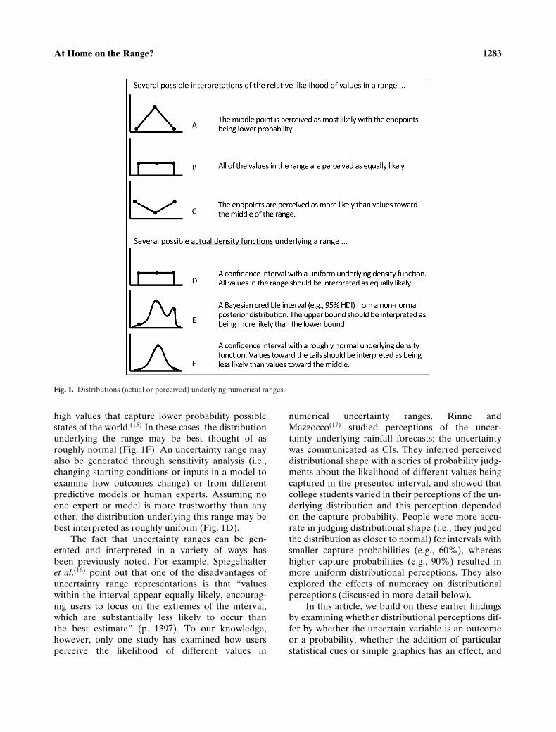
Decisionmakers may also focus on what therange reveals about the different possible states ofthe world and consider the likelihood of the differentvalues in the range. For instance, the IPCC tempera-ture forecast can be viewed as a range of possible fu-tures. One user may focus on the middle of the range

because she interprets the endpoints as describinglower probability events (Fig. 1A). Another usermay perceive the range as coming from a uniformdistribution, with all values in the range equally likelyto occur (Fig. 1B); in this case, it may not be clearwhere he will focus. Other interpretations are alsopossible, for example, with one end of the range per-ceived as more likely than the other, or with the end-points perceived as the most likely values (Fig. 1C).

Each interpretation implies different influencesof the forecast on judgments and decisions, par-ticularly in those contexts where the probabilityof extreme events is a critical consideration indetermining action. Take the excerpt from the IPCCreport above that forecasts a 2.5–10 °F increase intemperature over the next century. A decisionmakerdeliberating about different carbon emission reduc-tion strategies may feel a different sense of urgencydepending on whether she perceived the likelihoodof a 10° increase as a very low probability event oras just as likely as any other value in the range.

The correct interpretation of an uncertaintyrange will depend on how it was generated. Analystsworking in the frequentist statistical tradition oftenuse CIs to express precision in parameter estimation(e.g., 95% CI). Strictly speaking, a 95% CI, becauseit is derived from a sampling distribution, providesthe proportion of intervals in the long run that willinclude the parameter value (in this case, 95% ofthe intervals). Although a frequentist CI does notprovide specific information about the probabilityof occurrence for different values in the range, thetrue value is still more likely to be captured near thecenter of the CI than near the extremes.(13) Credibleintervals (or highest density intervals) generatedwith Bayesian statistical methods provide moreinformation. The credible interval is a summaryrepresentation of the full posterior probabilitydistribution, which represents the probability of eachpossible value for the parameter.(14) Thus, the correctinterpretation of the values in an uncertainty rangegenerated with these methods is directly related tothe shape of the underlying posterior distribution.Figs. 1D–1F show three different possible distribu-tions that could underlie a numerical uncertaintyrange based on a formal statistical analysis.

Uncertainty ranges can also be derived outsideof a formal statistical analysis. Ranges derived fromexpert judgment(s) are a case in point. In someapplications, an expert may be asked to provide aninterval estimate for a quantity that consists of a bestestimate (highest probability) along with low and

At Home on the Range? 1283

Fig. 1. Distributions (actual or perceived) underlying numerical ranges.

high values that capture lower probability possiblestates of the world.(15) In these cases, the distributionunderlying the range may be best thought of asroughly normal (Fig. 1F). An uncertainty range mayalso be generated through sensitivity analysis (i.e.,changing starting conditions or inputs in a model toexamine how outcomes change) or from differentpredictive models or human experts. Assuming noone expert or model is more trustworthy than anyother, the distribution underlying this range may bebest interpreted as roughly uniform (Fig. 1D).

The fact that uncertainty ranges can be gen-erated and interpreted in a variety of ways hasbeen previously noted. For example, Spiegelhalteret al.(16) point out that one of the disadvantages ofuncertainty range representations is that “valueswithin the interval appear equally likely, encourag-ing users to focus on the extremes of the interval,which are substantially less likely to occur thanthe best estimate” (p. 1397). To our knowledge,however, only one study has examined how usersperceive the likelihood of different values in

numerical uncertainty ranges. Rinne andMazzocco(17) studied perceptions of the uncer-tainty underlying rainfall forecasts; the uncertaintywas communicated as CIs. They inferred perceiveddistributional shape with a series of probability judg-ments about the likelihood of different values beingcaptured in the presented interval, and showed thatcollege students varied in their perceptions of the un-derlying distribution and this perception dependedon the capture probability. People were more accu-rate in judging distributional shape (i.e., they judgedthe distribution as closer to normal) for intervals withsmaller capture probabilities (e.g., 60%), whereashigher capture probabilities (e.g., 90%) resulted inmore uniform distributional perceptions. They alsoexplored the effects of numeracy on distributionalperceptions (discussed in more detail below).

In this article, we build on these earlier findingsby examining whether distributional perceptions dif-fer by whether the uncertain variable is an outcomeor a probability, whether the addition of particularstatistical cues or simple graphics has an effect, and


whether numeracy matters (as a main effect or in in-teraction with our other manipulations). We presentthree studies designed to improve understanding ofhow different characteristics and formats of the un-certain variables affect distributional perceptions.

2.1. Will Distributional Perceptions Differ if theUncertain Variable is an Outcomeor a Probability?

Lay users are likely to encounter uncertaintyin forecasted outcomes (e.g., the expected numberof fish, global temperature, etc.) and in assessedprobabilities (e.g., the probability of a surgical siteinfection). It is unclear whether distributional per-ceptions associated with outcome ranges versusprobability ranges are similar. To our knowledge,previous research has not explored possible similar-ities and differences. We expect these perceptionsto be similar, but differences could arise due to laypeoples’ difficulties with probabilities,(18) especiallyamong less numerate individuals. For example,individuals’ discomfort thinking about probabilitiescould mean that it is easier to conceptualize prob-ability ranges as being a range of equally probablelikelihood assessments obtained from a range ofexperts. However, it is also possible that individualdifferences and other format characteristics arethe more important contributors to distributionalperceptions and no significant differences betweenoutcome and probability ranges will be observed.We examine these competing possibilities in Study 1and expand on numeracy-related hypotheses below.

2.2. Does the Addition of Statistical Cues to RangesAffect Distributional Perceptions?

Ideally, the precise interpretation of any nu-merical range would be expressed clearly. However,communicators often do not have the luxury ofpresenting a detailed description of the elements ina display due to time or space constraints. Even ifthey did, the added detail might confuse rather thaninform.(19) In these cases, the user is left to interpretthe values in a range as he or she sees fit. A naturalbut rarely tested assumption is that the user willperceive the range in the way that the communicatorintended. Even if that approach is not thought tobe effective, analysts and other communicators maythink that providing statistical cues such as a “bestestimate” will be sufficient; this assumption has notbeen tested to the best of our knowledge.

A “best estimate” is typically presented as a sin-gle number supplemented with high- and low-endpoints. It is intended to imply to users that it is alsothe most likely value; that is, the value that will oc-cur with the highest probability. We therefore ex-pect that the presence of an explicit best estimate willmake it more likely that individuals perceive the dis-tribution to be roughly normal (Fig. 1F).

A second common cue is the capture probabil-ity of the numerical range. For example, describing arange as a “90% CI” may prompt people to believethat formal statistical methods were used to createthe range, and that the correct distributional inter-pretation is roughly normal or bell-shaped. In Study2, we hypothesize that:

H1: People will be more likely to report aroughly normal distributional interpretationwhen a range includes a best estimate and/ora description of capture probability (e.g.,90% CI).

2.3. Does Numeracy Influence DistributionalAssumptions?

An individual difference factor that has beenshown to moderate the use and interpretation of nu-merical information is numeracy. Numeracy refersto an individual’s ability to evaluate, transform,and use numerical information in common rea-soning and decision-making tasks.(18,20,21) Studieshave shown that numeracy affects the basic evalua-tion of numbers, choice strategies, risk perceptions,and the relative use of numeric and nonnumericinformation.(4,19,22)

One goal of this work was to explore whetherpeople who vary in numeracy systematically differin their perceptions of the distribution underlyingnumerical ranges. We hypothesize that more nu-merate participants would be more likely to per-ceive a roughly normal distribution. This expectationis based on the notion that more numerate peoplewould be more likely to have been exposed to sta-tistical concepts (e.g., the classic bell-shaped curve)and to use statistics.(23,24) Rinne and Mazzocco(17)

found mixed results in the one domain they exam-ined. In particular, more numerate participants hadmore normal distributional perceptions (which weremore accurate), but they were also more likely thanthe less numerate to perceive an inaccurate uniformdistribution. In Study 3, we provide further tests of


the relation between numeracy and distributionalperceptions in two different forecast domains.

H2: More numerate participants will be morelikely than the less numerate to perceive thedistribution underlying a numerical range asnormal as opposed to uniform (or other id-iosyncratic interpretations).

2.4. Do Simple Graphical RepresentationsDecrease the Variance in DistributionalPerceptions?

In many contexts, simple graphics can be addedto help decisionmakers interpret uncertainty ranges.A simplified density plot that shows the rough prob-ability of each value in the range would be a naturaloption. To the extent that people can understand thedensity representation, this would be a simple way toincrease the likelihood that people infer the correctdistribution, whether it is roughly normal, uniform,or some other shape.

Another graphical representation that has beensuggested for communicating uncertainty is theboxplot.(25) This representation shows the medianand 25th and 75th percentiles, along with the min-imum and maximum values. Because of this, assum-ing the distribution is symmetrical, a boxplot does notallow the user to distinguish between a roughly nor-mal, uniform, or bimodal distribution. For this rea-son, we do not expect the boxplot to decrease thevariance in distributional perceptions, at least if par-ticipants are drawing the appropriate inferences fromthis display. Thus, we expect the boxplot to produceperceptions of distributional shape that are indistin-guishable from a simple range.

In Study 3, we focus on a simple normal densitygraphic for communicating distributional informa-tion in a sample with a wide range of educationand numeracy skills. However, it is possible that themere presence of a statistical graphic would increaseperceptions of a normal distribution because of alay assumption that formal statistical methods arebeing used. Thus, without a comparison graphic, itwould be difficult to distinguish whether people aredrawing the appropriate meaning from the normaldensity plot or just responding to the presence of astatistical graphic. The boxplot graphic will allow usto tease apart these explanations because it does notprovide information to distinguish between differenttypes of symmetric distributions. Thus, if we seethe expected effects for the normal density plot and

not for the boxplot, we can be more confident thatthis effect is mediated by an understanding of thedensity plot and not just a general statistical grapheffect.

H3: The use of a normal density graphic willincrease perceptions of a normal distributionunderlying the uncertainty range compared toa nongraphical numerical uncertainty rangeor a boxplot graphic.

H4: The boxplot graphic will not significantlychange distributional perceptions as com-pared to a nongraphical numerical uncer-tainty range.

3. STUDY 1

In Study 1, we examined how lay people perceivethe distribution underlying numerical ranges and ex-plored our first research question, namely, whetherpeople will perceive numerical ranges any differentlyif the uncertain variable is a probability as opposedto an outcome.

This study was conducted in an environmentalrisk management decision-making context. As de-scribed below, participants were presented with ascenario describing options for reducing the numberand magnitude of wildfires and a consequence tablethat summarized the anticipated impact of differentmanagement options.(10) As is often the case in prac-tice, the attributes that differentiate the managementoptions are estimated with uncertainty that needs tobe communicated to decisionmakers.

3.1. Sample

Participants (N = 165) were randomly drawnfrom the Decision Research web panel subjectpool. The mean age of the sample was 40 years(range = 19–71 years) and was 58% female. Approxi-mately 25% had a high school education or less, 32%had attended some college or vocational school, 33%were college graduates, and 10% had advanced de-grees.

3.2. Design and Measures

Participants completed a short tutorial that de-scribed the nature and purpose of consequencetables. They then answered several comprehensionquestions to confirm that they could interpret theinformation in a practice consequence table before


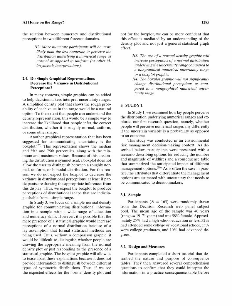
Fig. 2. Study 1: Scenario and consequence tables.

proceeding with the study. Participants were thenpresented with a scenario describing the dangers ofhuman-caused forest fires and a broad goal for reduc-ing the number of acres burned per year. Three dif-ferent environmental management options were thenoutlined in a standard consequence table (see Fig. 2).Note that a “best estimate” for each option is alwaysprovided.

The nature of the uncertain variable was ma-nipulated in a two-group (outcome vs. probability)between-subjects design. In the outcome condition,performance of the different land managementoptions was communicated through the reduction

in annual average acres burned. In the probabilitycondition, performance was communicated by ex-pressing the probability (in % form) of successfullyreducing acres burned by 175K (i.e., the broad goaloutlined in the narrative introduction). Participantswere then asked about their perceptions of the distri-bution underlying the numerical ranges: “Considerthe confidence ranges shown in the consequencetable. Do you think that all of the values withinthese ranges are equally likely, or do you think someare more likely than others? (a) All are equallylikely, (b) The values closer toward the middle ofthe range are more likely than those at the ends ofthe range, and (c) The values toward the ends of therange are more likely than those closer toward themiddle.”

3.3. Results and Discussion

Participants were most likely to interpret thevalues within the confidence range as being uniform(48.8%), with a smaller percentage perceiving aroughly normal shape (40.2%), and a minorityperceiving values further from the best estimate asbeing more likely (U-shaped; 11.0%). That a sizableminority of participants (11%) perceived the endsof the range to be more likely in the presence a“best” estimate is somewhat alarming given thatthis is very unlikely to be a correct distributionalinterpretation. Multinomial logistic regression wasused to test for differences in perceptions acrossconditions (see Fig. 3). Distributional perceptionsdid not significantly differ by condition, χ2(2) = 2.45,p = 0.20, nor were they related to age, gender, oreducation level of the participants. Overall, we foundno evidence that distributional perceptions in thisenvironmental choice task were related to whetherthe uncertain variable was a probability or anoutcome.

In Study 2, we attempted to replicate these gen-eral trends in distributional perceptions and to testH1—that people will be more likely to report aroughly normal distributional interpretation when arange includes a best estimate and/or a description ofcapture probability (e.g., 90% CI).

4. STUDY 2

In Study 2, we examined the generalizability ofdistributional perceptions, this time in the contextof a climate change forecast. We expected this typeof forecast to be more familiar to many participants


Fig. 4. Study 2: Climate change fore-casts shown in each experimental con-dition.

Fig. 3. Study 1: Distributional perceptions by experimental condi-tion.Note: Bars are 95% confidence intervals.

than the earlier forest fire forecast because climatechange forecasts are often presented in media reportswith numerical uncertainty ranges. We also testedwhether lay people would be more likely to perceiveranges that included a best estimate and/or a descrip-tion of capture probability (e.g., 90% CI) as roughlynormally distributed (H1).

4.1. Sample

Participants (N = 89; 64% female) were ran-domly drawn from the Decision Research web panel

subject pool. The mean age of the sample was40 years (range = 21–66 years). Approximately 20%had a high school education or less, 30% attendedsome college or vocational school, 30% were collegegraduates, and 20% had advanced degrees.


Participants were presented with climate changeforecasts in a 2 (best estimate or not) × 2 (90% CIor range format) mixed experimental design. Thepresence versus absence of the best estimate wasa within-subjects factor (order counterbalanced)and the description of the range was manipulatedbetween subjects (presence vs. absence of a 90% CI;see the four conditions described in Fig. 4).

Participants were then asked about their per-ceptions of the distribution underlying the numericalrange with the same question and response optionsas in Study 1.

4.3. Analytic Approach

The primary analyses were conducted with ageneralized mixed effects modeling approach imple-mented in the lme4 package for the R statisticalcomputing environment.(26) The dependent variablewas binary (uniform vs. normal distributional per-ception) and the between- and within-subject fac-tors as well as their interaction were entered aspredictors.


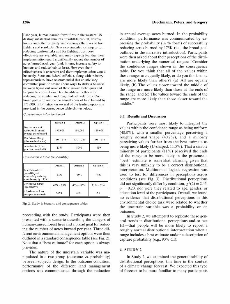
Fig. 5. Study 2: Distributional perceptions by experimental condition.Note: Bars are 95% confidence intervals.


Study 2 participants differed in their perceptionsof the distributions underlying numerical rangesacross the conditions (see Fig. 5). A roughly normaldistribution was the modal response as opposedto a uniform distribution in Study 1. A randomintercepts model adequately described the datastructure (adding a random effect for slope did notsignificantly improve fit, p = 0.95). The odds ofperceiving a normal distribution were 2.27 timesgreater when the best estimate was present versusabsent, odds ratio = 2.27, p = 0.02. The main effectof the presence versus absence of the 90% CI wasnot significant but was in the expected direction,odds ratio = 1.80, p = 0.13. Thus, H1 received partialsupport.

Two patterns stand out in Fig. 5: (1) participantsin the no-CI and no-best estimate condition weremore likely to perceive the distribution as uniformthan normal, in contrast to the other conditions,and (2) participants were least likely to perceivea u-shaped distribution but were more likely toperceive it when no best estimate was presented.As expected, the cross-level interaction effect addedpredictive power to the model, χ2(1) = 4.50, p =0.03, confirming what is apparent in Fig. 5 that par-ticipants were significantly more likely to perceive auniform distribution when the range was presented

without a best estimate and without a CI description,in contrast to the other three conditions.

McNemar’s test for dependent proportions wasused to test whether the u-shaped distributional per-ception was more likely when no best estimate waspresented (averaging across the between-subjectscondition). Although the effect was relatively small,people were more likely to perceive the underlyingdistribution to be u-shaped when no best estimatewas presented (13.8% vs. 5.8%), Diff (unsigned) =0.08, p = 0.04.

These results are broadly consistent with H1 andsuggest that people are sensitive to the presence ofspecific statistical cues concerning the interpretationof values in a numerical range. When the fewestnumber of statistical cues were present (i.e., whenthere was no best estimate or CI description), par-ticipants were significantly more likely to perceivethe range as uniform. As in Study 1, a sizeableminority (up to 18% in one condition) perceived au-shaped distribution, and this effect was magnifiedwhen a best estimate was not displayed. This is acompelling result because it would be exceedinglyrare for this to be the correct interpretation of anumerical uncertainty range. Given that the pres-ence of a statistical cue (the best estimate) reducedu-shaped interpretations, the results also suggestthat these nonnormative interpretations were not


necessarily due to inattention but were, at least inpart, a reaction to the information presented.

However, interpretation of the u-shaped dis-tributional response is ambiguous. To be classifiedas having a u-shaped perception, participants hadto have responded that “the values toward theends of the range are more likely than those closertoward the middle.” This response may mean thatthe individual thought the distribution was u-shapedor it may mean that the distribution was perceivedto be skewed in one direction and not the other.Equally problematic is that our response optionsdid not provide a clear choice for someone whoperceived the distribution to be skewed. In Study 3,we added a fourth “none of the above” option withan open-response field in an attempt to capture suchperceptions.

5. STUDY 3

In Study 3, we expanded our investigation bylooking at several simple and commonly used graph-ical representations—namely, simple density plotsand boxplots. We tested H3 (that providing simplenormal density plots would increase the proportionof the participants that accurately reports a normaldistribution compared to providing numerical rangeinformation only) and H4 (that the boxplot wouldnot significantly differ from the numerical range).Using the boxplot as a comparison served two pur-poses: (1) it acted as a control condition with whichto compare the effects of the simple normal density,in that we could ascertain whether the simple den-sity plot is being comprehended as opposed to it justhaving a general statistical graphic effect, and (2) theboxplot has recently been recommended as the bestway to present uncertainty in many domains.(25,27)

We also included both climate change and health sce-narios to increase the generalizability of these re-sults. Finally, we included a measure of numeracyand tested H2 (that the more numerate are morelikely to perceive a normal distribution).

5.1. Sample

Participants (N = 291; 54% female) were ran-domly drawn from the Decision Research web panelsubject pool. The mean age of the sample was45 years (range = 21–76 years). Approximately 28%had a high school education or less, 31% attended

some college or vocational school, 27% were collegegraduates, and 14% had advanced degrees.


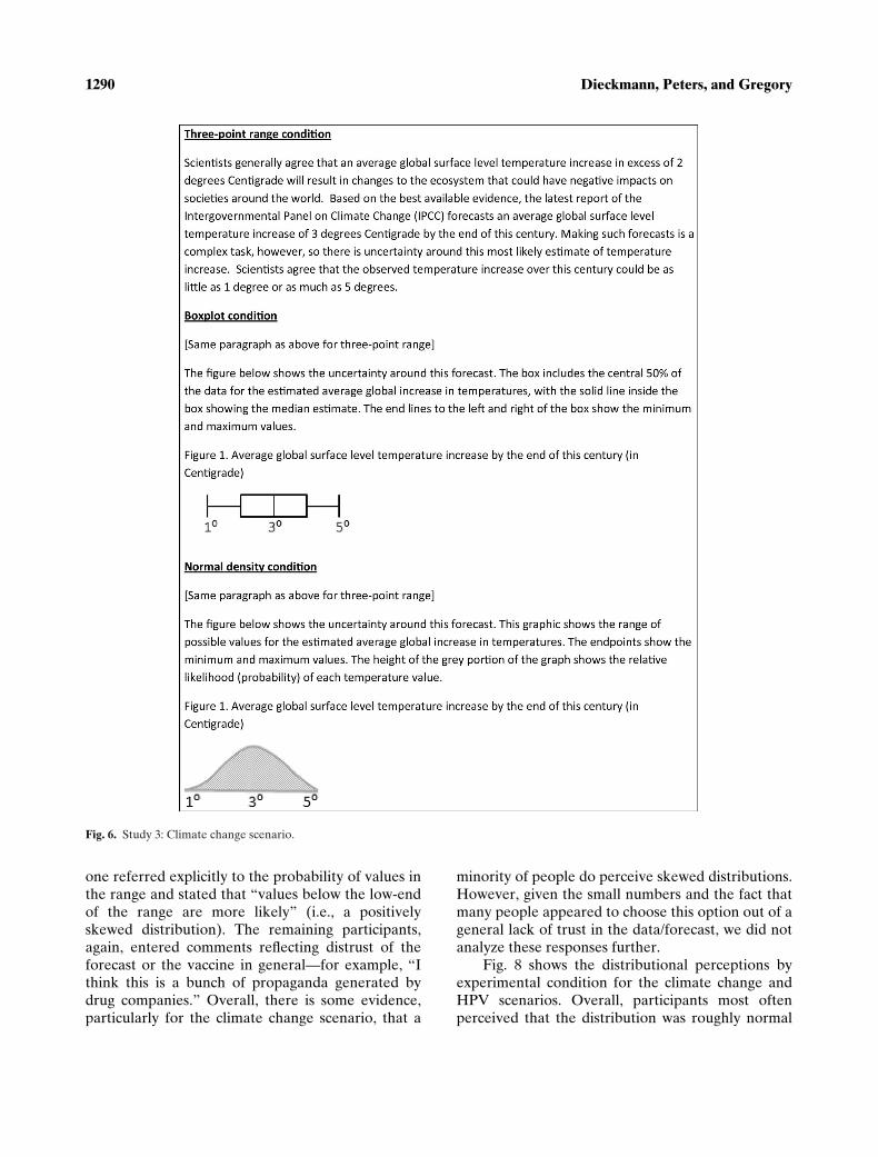
Participants were randomly assigned to one ofthe three uncertainty format groups (range, box-plot, or normal density) in a completely between-subjects design. Within each condition, participantsexamined two forecasts in sequential order. Thefirst forecast was in the climate change domain(see Fig. 6) and the second in the health domain(Human Papillomavirus (HPV) vaccination; seeFig. 7). After viewing each forecast, participants wereasked about their perceptions of the distributionunderlying the numerical range: “Do you think thatall of the values within this range are equally likely,or do you think some are more likely than others? (a)All are equally likely, (b) The values closer towardthe middle of the range are more likely than those atthe ends of the range, (c) The values toward the endsof the range are more likely than those closer towardthe middle, and (d) None of the above: Please spec-ify: ______________.” In a prior session (two weeksprior to the main experiment), participants com-pleted an eight-item numeracy measure.(28) Alphareliability was acceptable and the data were roughlynormally distributed (Mean = 3.79, Md = 4.0,Skew = 0.10, Kurtosis = –0.55. Alpha = 0.71).


Table I shows the distributional perceptions forboth scenarios averaged across the three experimen-tal conditions. Overall, participants were most likelyto perceive the distribution to be roughly normalin both scenarios. Unlike the previous studies, weincluded a “none of the above option” and provideda space for participants to elaborate in writing. Over-all, only 5.5% (n = 16) and 5.2% (n = 15) chose thisoption in the climate change and HPV vaccine sce-narios, respectively. For the climate change scenario,of the 13 people who provided written responses,five of them mentioned that they thought thatvalues toward the lower end of the range were morelikely (i.e., a positively skewed distribution). Theremaining participants provided comments reflectinga general lack of trust in the data or forecasters—forexample, “Don’t see how they can predict future,”“There is no accurate computer model for CC,”“Global warming is a total farce.” For the HPV sce-nario, of the 15 people who provided comments, only


Fig. 6. Study 3: Climate change scenario.

one referred explicitly to the probability of values inthe range and stated that “values below the low-endof the range are more likely” (i.e., a positivelyskewed distribution). The remaining participants,again, entered comments reflecting distrust of theforecast or the vaccine in general—for example, “Ithink this is a bunch of propaganda generated bydrug companies.” Overall, there is some evidence,particularly for the climate change scenario, that a

minority of people do perceive skewed distributions.However, given the small numbers and the fact thatmany people appeared to choose this option out of ageneral lack of trust in the data/forecast, we did notanalyze these responses further.

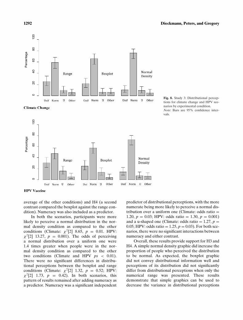
Fig. 8 shows the distributional perceptions byexperimental condition for the climate change andHPV scenarios. Overall, participants most oftenperceived that the distribution was roughly normal


Fig. 7. Study 3: HPV scenario.

across all conditions for both the scenarios. However,in the normal density condition, participants weremore likely to indicate that they perceived the distri-bution as normal and they were less likely to indicatethat they perceived it as uniform as compared to theother conditions. A multinomial logistic regressionmodel was used to compare the choice proportionsacross conditions for each scenario separately.Participants who responded “none of the above”were excluded for the purposes of this analysis. A set

Table I. Study 3: Distributional Perceptions for the ClimateChange and HPV Scenarios

Scenario Uniform Normal U-Shaped Other

Climate change 19.0% 67.2% 8.3% 5.5%HPV vaccine 23.1% 59.7% 12.1% 5.2%

of orthogonal contrasts were used to compare theexperimental conditions and test H3 (one contrastcompared the normal density condition against the


Fig. 8. Study 3: Distributional percep-tions for climate change and HPV sce-narios by experimental condition.Note: Bars are 95% confidence inter-vals.

average of the other conditions) and H4 (a secondcontrast compared the boxplot against the range con-dition). Numeracy was also included as a predictor.

In both the scenarios, participants were morelikely to perceive a normal distribution in the nor-mal density condition as compared to the otherconditions (Climate: χ2[2] 8.65, p = 0.01. HPV:χ2[2] 13.27, p = 0.001). The odds of perceivinga normal distribution over a uniform one were1.4 times greater when people were in the nor-mal density condition as compared to the othertwo conditions (Climate and HPV ps < 0.01).There were no significant differences in distribu-tional perceptions between the boxplot and rangeconditions (Climate: χ2[2] 1.32, p = 0.52; HPV:χ2[2] 1.73, p = 0.42). In both scenarios, thispattern of results remained after adding numeracy asa predictor. Numeracy was a significant independent

predictor of distributional perceptions, with the morenumerate being more likely to perceive a normal dis-tribution over a uniform one (Climate: odds ratio =1.20, p = 0.03; HPV: odds ratio = 1.30, p = 0.001)and a u-shaped one (Climate: odds ratio = 1.27, p =0.05; HPV: odds ratio = 1.25, p = 0.03). For both sce-narios, there were no significant interactions betweennumeracy and either contrast.

Overall, these results provide support for H3 andH4. A simple normal density graphic did increase theproportion of people who perceived the distributionto be normal. As expected, the boxplot graphicdid not convey distributional information well andperceptions of its distribution did not significantlydiffer from distributional perceptions when only thenumerical range was presented. These resultsdemonstrate that simple graphics can be used todecrease the variance in distributional perceptions


for people across a range of numeracy. In addition,we also provide support for H2, in that the morenumerate were more likely than the less numerateto report a normal distribution across conditions inboth the scenarios.

6. GENERAL DISCUSSION

In this article, we focused on the understudiedtopic of how lay people perceive the relative like-lihood of values in a numerical uncertainty range.This is important because decisionmakers who dif-fer in their distributional perceptions could come toquite different conclusions about the importance ofthe forecast as a whole and/or of the plausibility ofextreme events at the ends of a range. Our goal is tofurther document how people evaluate and use un-certainty in expert forecasts, thereby contributing toan improved understanding of how uncertainty canbe best communicated. The three primary themesfrom our findings are summarized below.

First, in four different scenarios ranging fromclimate change to HPV vaccination, we found sub-stantial variation in distributional perceptions. Mostpeople perceived either a roughly normal or uni-form distribution, but a substantial minority per-ceived a u-shaped or other distribution. We did notfind evidence that distributional perceptions were re-lated to the uncertain variable being a probability oran outcome. We did, however, find modest effectsof numeracy with respect to distributional percep-tions. More numerate participants were more likelythan the less numerate to perceive a normal distri-bution underlying a numerical range and they wereless likely than the less numerate to perceive a uni-form distribution. Unlike Rinne and Mazzocco,(17)

we found no evidence that the more numerate weremore likely to perceive uniform distributions.

Second, providing statistical cues (90% CI inStudy 2) and including a best estimate tended toprompt a roughly normal interpretation, whereasproviding a range without this information tendedto prompt a uniform or u-shaped interpretation.These findings are consistent with participants usingwhatever values are available to construct theirinterpretation (in this case, only the endpoints wereavailable; see work by Slovic(29) on the concretenessprinciple). Yet even in the presence of a best estimatethat provides a strong cue about the ends of the rangebeing less likely than the “best” estimate, a substan-tial proportion of participants nonetheless perceivedthe underlying distribution to be uniform. In other

words, these cues explained some, but by no meansall, of the variance in distributional perceptions.

These results highlight the flexibility of inter-pretations of seemingly “precise” numbers. Expertsare often told to avoid using verbal uncertaintyexpressions because people vary in how they inter-pret these phrases. However, just using numbersto express uncertainty is not enough to ensureaccurate interpretation. The present results suggestthat additional attention needs to be given to howuncertainty ranges are displayed and described, soas to minimize the variance in interpretation and tohelp end users make informed decisions.

Third, we demonstrated that a simple normaldensity plot accompanying the range decreased thevariance in distributional perceptions for peoplevarying in numeracy. Of course, many contexts existin which it might not be feasible to include a graphicand the text required to describe the properties ofthe graphic. However, even in these cases it might bepossible to include some supplementary information(e.g., perhaps short verbal descriptions of the distri-bution underlying the range) that increases the likeli-hood that users will make distributional perceptionsthat are more accurate and/or match the intentionsof the analyst. Future research should focus on com-paring the usefulness of simple verbal descriptions(e.g., “values at the ends of the range are less likelythan those towards the middle”) and alternativegraphical displays for communicating distributionalinformation.

Our results concerning graphical displays alsohave bearing on the oft-recommended boxplot dis-play for communicating uncertainty. Boxplots havemany desirable properties in that particular types ofinformation are very salient (e.g., the 25th and 75thpercentile and extreme values). Our results, how-ever, highlight a limitation in their use. We thereforequestion the appropriateness of using classic box-plots without additional information that makes theunderlying distribution salient (e.g., verbal descrip-tion or some other graphic device). It will be left tofuture work to determine whether the advantages ofboxplots as a device for communicating uncertaintyoutweigh the limitations they have in communicatingdistributional information.

Finally, a host of other factors, includingworldviews(30) and mental models,(31) also may af-fect distributional perceptions. It may be that whenuncertainty ranges are left ambiguous as to the cor-rect distributional interpretation, people may be mo-tivated to choose an interpretation that best fits with


what they want to believe. For instance, a personskeptical of climate science may perceive uncertaintyranges to be roughly uniform or positively skewedbecause this interpretation is consistent with temper-ature increases at the low end of the range beingequally or potentially more probable than moderateto large increases. In a companion paper, we presentexperimental evidence that this motivated processingof range information does, in fact, occur under somecircumstances and can be lessened by reducing theinterpretational ambiguity of the numerical range.(32)

Several factors limit the strength of the infer-ences that can be drawn from these experiments. Themultiple choice question format may have promptedparticipants to report distributional perceptions thatthey otherwise would not have considered when justevaluating the range or graphical displays. As wediscuss in Section 1, whether the relative likelihoodof values within a range is initially considered islikely related to the sense-making strategy employedby the end user. However, even in the presenceof a potentially leading multiple choice questionwe still show substantial variance in distributionalperceptions. Although not examined in these studies,it seems likely that decisionmakers’ distributionalperceptions will affect choices, particularly in con-texts where the probability of extreme events iscritical to a decision. Future studies should focus ondelineating when and how distributional perceptionsaffect choice behavior in a range of representativetasks.

Another potential limitation of this work is thatthe self-report approach to assessing distributionalperceptions only allowed us to get at rough per-ceptions of the likelihood of different values in therange (e.g., are values at the ends equally or lesslikely than those toward the middle?). In contrast,the method used by Rinne and Mazzocco(17) wasbased on a series of probability judgments aboutthe likelihood of different values within the range.This approach allowed a more precise estimationof the perceived distribution (e.g., t-distribution ascompared to normal). Their approach, however,relies on lay people being able to make precise andconsistent probability judgments with which they aremost likely unfamiliar. We believe that our moregist-based approach was appropriate in this contextas it better approximates the level of abstractionthat lay people use when making judgments anddecisions. Regardless, both elicitation methods likelyhave advantages and drawbacks and would ideallybe combined in future studies in this area.

7. CONCLUSIONS

The practical implications of this work arestraightforward. To a far greater degree than is typi-cally done, risk analysts and group facilitators shouldprovide detailed descriptions about how to interpretnumerical uncertainty ranges. Providing statisticalcues such as best estimates are helpful, but our resultsshow that there is still a great variance in interpre-tation even when these cues are provided. In manyapplications, we expect that analysts and decision-makers will be working either with numerical rangesthat constitute a series of equally plausible values(e.g., estimates from competing computer modelsor from multiple human experts), or with roughlynormal ranges that have extreme values (at the highand low ends) that are less likely than values towardthe middle. Better communication with users aboutthe interpretation of numerical ranges will minimizeincorrect interpretations and reduce the likelihood ofend users basing interpretations on irrelevant infor-mation or other potentially biasing preconceptions.

We will, of course, never be able to completelyeliminate interpretational errors concerning uncer-tainty. However, significant opportunities exist toimprove uncertainty communication and maximizethe likelihood that users will make accurate evalu-ations of uncertain quantities and then incorporatethis information into their deliberations. In highlycharged domains characterized by substantial uncer-tainty, such as climate change, any changes that couldbe made to help facilitate communication and im-prove understanding among stakeholders would bewell worth the effort.

ACKNOWLEDGMENTS

We acknowledge the generous support of theU.S. National Science Foundation: Awards 0925008,1231231, 1155924, SES-1047757, SES-0728934, andSES-0901036. The views expressed in this article arethose of the authors alone, with the exception ofportions of the article’s title, which we share withMorgenstern et al. (2013).

REFERENCES

1. National Aeronautics and Space Administration. The currentand future consequences of global change, n.d. Available at:http://climate.nasa.gov/effects, Accessed August 18, 2013.

2. Dieckmann NF, Slovic P, Peters E. The use of narrative ev-idence and explicit likelihood by decision makers varying innumeracy. Risk Analysis, 2009; 29:1473–1488.


3. Budescu DV, Broomell S, Por HH. Improving communicationof uncertainty in the reports of the Intergovernmental Panelon Climate Change. Psychological Science, 2009; 20:299–308.

4. Dieckmann NF, Mauro R, Slovic P. The effects of presentingimprecise probabilities in intelligence forecasts. Risk Analysis,2010; 30:987–1001.

5. Dieckmann NF, Peters E, Gregory R, Tusler M. Making senseof uncertainty: Advantages and disadvantages of providing anevaluative structure. Journal of Risk Research, 2012; 15:717–735.

6. Du N, Budescu DV, Shelly MK, Omer TC. The appeal ofvague financial forecasts. Organizational Behavior and Hu-man Decision Processes, 2011; 114:179–189.

7. Durbach IN, Stewart TJ. An experimental study of the effectof uncertainty representation on decision making. EuropeanJournal of Operational Research, 2011; 214:380–392.

8. Joslyn S, Savelli S, Nadav-Greenberg L. Reducing probabilis-tic weather forecasts to the worst-case scenario: Anchoringeffects. Journal of Experimental Psychology-Applied, 2011;17:342–353.

9. Joslyn SL, LeClerc JE. Uncertainty forecasts improveweather-related decisions and attenuate the effects offorecast error. Journal of Experimental Psychology-Applied,2012; 18:126–140.

10. Gregory R, Dieckmann NF, Peters E, Failing L, Long G,Tusler M. Deliberative disjunction: Expert and public un-derstanding of outcome uncertainty. Risk Analysis, 2012;32:2071–2083.

11. Mellers BA, Richards V, Birnbaum MH. Distributional the-ories of impression formation. Organizational Behavior andHuman Decision Processes, 1992; 51:313–343.

12. Ellsberg D. Risk, ambiguity, and the savage axioms. QuarterlyJournal of Economics, 1961; 75:643–669.

13. Cumming G, Finch S. Inference by eye: Confidence intervalsand how to read pictures of data. American Psychologist, 2005;60:170–180.

14. Kruschke JK. Doing Bayesian Data Analysis: A Tutorialwith R and BUGS. Burlington, MA: Academic Press/Elsevier,2011.

15. Speirs-Bridge A, Fidler F, McBride M, Flander L, CummingG, Burgman M. Reducing overconfidence in the interval judg-ments of experts. Risk Analysis, 2010; 30:512–523.

16. Spiegelhalter DJ, Short I, Pearson M. Visualizing uncertaintyabout the future. Science, 2011; 333:1393–1400.

17. Rinne LF, Mazzocco MMM. Inferring uncertainty from inter-val estimates: Effects of alpha level and numeracy. Judgmentand Decision Making, 2013; 8:330–344.

18. Reyna VF, Nelson WL, Han PK, Dieckmann NF. How numer-acy influences risk comprehension and medical decision mak-ing. Psychological Bulletin, 2009; 135:943–973.

19. Peters E, Dieckmann NF, Dixon A, Hibbard JH, Mertz CK.Less is more in presenting quality information to consumers.Medical Care and Research Review, 2007; 64:169–190.

20. Peters E, Hibbard JH, Slovic P, Dieckmann NF. Numeracyskill and the communication, comprehension, and use of risk-benefit information. Health Affairs (Millwood), 2007; 26:741–748.

21. Peters E, Vastfjall D, Slovic P, Mertz CK, Mazzocco K,Dickert S. Numeracy and decision making. Psychological Sci-ence, 2006; 17:407–413.

22. Peters E. Beyond comprehension: The role of numeracy injudgments and decisions. Current Directions in PsychologicalScience, 2012; 21:31–35.

23. Chesney DL, Obrecht NA. Statistical judgments are in-fluenced by the implied likelihood that samples representthe same population. Memory and Cognition, 2012; 40:420–433.

24. Obrecht NA, Chesney DL. Sample representativeness affectswhether judgments are influenced by base rate or sample size.Acta Psychologica (Amst), 2013; 142:370–382.

25. Fischhoff B. Communicating uncertainty: Fulfilling the dutyto inform. Issues in Science and Technology (serial onthe Internet). 2012: Available at: http://www.issues.org/28.4/fischhoff.html.

26. R Development Core Team. R: A Language and Environmentfor Statistical Computing. Vienna, Austria: R Foundation forStatistical Computing, 2008.

27. Morgan MG, Dowlatabadi H, Henrion M, Keith D, Keith D,Lempert R, McBride S, Small M, Wilbanks T. Best practiceapproaches for characterizing, communicating and incorporat-ing scientific uncertainty in climate decision making (ReportNo. CCSP 5.2) 2009, January. Available at: http://www.climatescience.gov/Library/sap/sap5-2/sap5-2-final-report-all.pdf.

28. Weller JA, Dieckmann NF, Tusler M, Mertz CK, Burns WJ,Peters E. Development and testing of an abbreviated numer-acy scale: A Rasch analysis approach. Journal of BehavioralDecision Making, 2013; 26:198–212.

29. Slovic P. From Shakespeare to Simon: Speculation—and someevidence—about man’s ability to process information. OregonResearch I Research Monograph, 1972; 12(2):1–29.

30. Douglas M, Wildavsky A. Risk and Culture: An Essay on theSelection of Technical and Environmental Dangers. Berkeley:University of California Press, 1982.

31. Morgan MG, Fischhoff B, Bostrom A, Atman CJ. RiskCommunication: A Mental Models Approach. New York:Cambridge University Press, 2002.

32. Dieckmann NF, Peters E, Gregory R. Seeing what you wantto see: How imprecise uncertainty ranges enhance motivatedcognition. Risk Analysis 2014, under review.

At Home on the Range? Lay Interpretations of...

Documents

Transcript of At Home on the Range? Lay Interpretations of...