Asymptotic Performance of a Censoring Sensor Network

IEEE TRANSACTIONS ON INFORMATION THEORY, VOL. 53, NO. 11, NOVEMBER 2007 4191

Asymptotic Performance of a CensoringSensor Network

Wee Peng Tay, Student Member, IEEE, John N. Tsitsiklis, Fellow, IEEE, and Moe Z. Win, Fellow, IEEE

Abstract—We consider the problem of decentralized binarydetection in a sensor network where the sensors have access to sideinformation that affects the statistics of their measurements, or re-flects the quality of the available channel to a fusion center. Sensorscan decide whether or not to make a measurement and transmit amessage to the fusion center (“censoring”), and also have a choiceof the mapping from measurements to messages. We consider thecase of a large number of sensors, and an asymptotic criterioninvolving error exponents. We study both a Neyman–Pearson anda Bayesian formulation, characterize the optimal error exponent,and derive asymptotically optimal strategies for the case wheresensor decisions are only allowed to depend on locally availableinformation. Furthermore, we show that for the Neyman–Pearsoncase, global sharing of side information (“sensor cooperation”)does not improve asymptotic performance, when the Type I erroris constrained to be small.

Index Terms—Censoring, cooperation, decentralized detection,error exponent, sensor networks.

I. INTRODUCTION

Asensor network is often constrained by energy limitations,because the sensors are typically low-cost battery-pow-

ered devices, and by communication limitations, because oftransmission costs or limited available radio resources. Whendeploying a large-scale sensor network for the purposes ofdetection, e.g., for environmental monitoring or for detectinganomalies in industrial applications, we are often faced with atradeoff between energy efficiency and detection reliability. Toaddress this issue, “censoring networks” have been introducedin [1] and later in [2]. These references consider a binary de-tection problem, assume that the sensors obtain independentmeasurements , and raise the question of deciding whichsensors should transmit their measurements to a fusion center,subject to a constraint on the average number of transmittingsensors. In particular, they assume that the sensors are operatingindependently from each other, i.e., the censoring decisions donot involve any sensor cooperation or exchange of information.Their main results state that each sensor should base its deci-sion on the likelihood ratio associated with its measurement,

Manuscript June 30, 2006; revised June 2, 2007. This work was supported,in part, by the National Science Foundation under Contracts ECS-0426453 andANI-0335256, the Charles Stark Draper Laboratory Robust Distributed SensorNetworks Program, and an Office of Naval Research Young Investigator AwardN00014-03-1-0489. The material in this paper was presented in part at the Con-ference on Information Sciences and Systems, Princeton, NJ, March 2006 andIEEE International Symposium on Information Theory, Seattle, WA, July 2006.

The authors are with the Laboratory for Information and Decision Systems,the Massachusetts Institute of Technology, Cambridge, MA 02139 USA (e-mail:[email protected]; [email protected]; [email protected]).

Communicated by A. Høst-Madsen, Associate Editor for Detection and Es-timation.

Digital Object Identifier 10.1109/TIT.2007.907441

and should transmit only if the likelihood ratio falls outsidea “censoring interval.” Subsequently, [3] and [4] consider theasymptotic performance of “constrained networks,” includingthe case of an overall power constraint and the case of ca-pacity-constrained communications. The question of decidingwhich sensors should transmit is replaced by the question ofchoosing the mode of sensor transmissions. There are differ-ences between the problems considered in [1] and the problemsstudied in [3] and [4], but there are also significant similarities,suggesting that a unified treatment may be possible. Such aunified treatment, at a higher level of generality, is one of theobjectives of this paper. However, we will be concerned withsensor networks with an asymptotically large number of nodes,unlike in [1], [2], where the problem of censoring is treated forthe case of a fixed number of nodes. In particular, we providea formulation that involves:

1) a general class of “network constraints,”2) a general class of possible “transmission modes” that the

sensors can choose from, and3) the possibility of having access to some side information

, which can be used to choose between transmissionmodes.

We use the term “side information” in a very general wayto refer to some observable that affects the operation of eachsensor. In general, could provide information on the qualityof the channel from sensor to the fusion center, or on thequality of the measurement available at sensor . The choiceof what side information is available depends on the specificproblem and its constraints. We illustrate our framework by pre-senting two motivating examples, which will be revisited in Sec-tion VIII.

Example 1 (Fading Channels): Consider a large number ofsensors deployed for the purposes of detection, that is, testingbetween two hypotheses and . Each sensor obtainsan independent measurement (with a different distributionunder each hypothesis), which it can encode and transmit to afusion center through a noisy channel. The message received atthe fusion center is of the form

where is a stochastic fading coefficient, and is zero-meanGaussian noise with known variance , independent of every-thing else. In order to conserve power, or to avoid divulging thepresence of the sensors, we introduce a constraint that under“normal conditions” (that is, under the null hypothesis ),the expected number of transmitting sensors is bounded by ,where is a given constant. Then, the sensor network

0018-9448/$25.00 © 2007 IEEE

4192 IEEE TRANSACTIONS ON INFORMATION THEORY, VOL. 53, NO. 11, NOVEMBER 2007

is faced with the problem of choosing which sensors shouldtransmit their measurements to the fusion center. Suppose thatthe network has knowledge of the channel state informationand , . Obviously, we would like to choose onlythose sensors that have a favorable channel to the fusion center,so the choice should be based on . (In some cases,

is a known constant, then the choice is made based only on.) Furthermore, we would like to examine and compare

a cooperative scheme (the decision to transmit or not by eachsensor depends on the channel parameters of all sensors) and adistributed scheme (the decision of each sensor depends only onthe local channel parameters). Finally, we may want to optimizethe choice of the “transmission function” from within a classof possible such functions.

Example 2 (Spatial Signal): Consider the problem of de-tecting a spatial signal on the domain (or more generallyon a bounded subset of ). The sensors are placed randomlyand uniformly in the set , with the fusion center at theorigin. Let be the location of sensor . This serves as theside information that is available. There are two possible spa-tial signals and , and we wish to detect which of thetwo is present. Each sensor makes a noisy measurement of thelocal signal. We assume that the power required for a sensorto transmit its measurement depends on the distance from thesensor to the fusion center. Given a constraint on the total powerused by the sensors, which ones should be chosen to transmit? Itis not necessarily the case that the sensors closest to the fusioncenter should be the ones transmitting; for instance, if the spa-tial signals and are equal when is in the vicinityof the fusion center, the sensors close to the fusion center do nothave any information worth transmitting. In Section VIII-B, wewill give an example where the transmitting sensors should bethe ones furthest away from the fusion center.

In this paper, we provide a framework that is general enoughto address the questions posed in the above examples. In partic-ular, we generalize the idea of a censoring network presented in[1], and introduce network constraints in the spirit of [3] and [4].To be specific, we consider a Neyman–Pearson decentralizedbinary detection problem where the sensors utilize side infor-mation when deciding to transmit their measurements to thefusion center. We introduce a cost function that depends onlyon the side information and the transmission policy used, andrequire that the expected average cost per sensor be below agiven threshold. Finding an optimal solution to such a problemis rather intractable. For this reason, we focus on an asymptoticanalysis, involving a large number of sensors and the minimiza-tion of the error exponent, in the spirit of [5], which introducedand studied such a formulation in the context of unconstrainedsensor networks.

In our formulation, we allow the sensors to cooperate, in thesense that the sensors’ censoring decisions can be made by thefusion center, on the basis of the entire vectorof side-information values at each sensor. This can arise, forexample, when the local pieces of side information are somelow-resolution data that can be transmitted to the fusion centerinexpensively, or when the fusion center is able to monitor thestate of the channels from the sensors to itself. Nevertheless, we

will establish that when the Type I error probability is asymp-totically small, optimal performance can be achieved even inthe absence of such cooperation, by having each sensor makeits censoring and transmission decisions only on the basis ofthe locally available side information. Furthermore, all the sen-sors can use the same policy, which shows that a simple dis-tributed scheme is asymptotically optimal. The case where thereis no cooperation is the asymptotic counterpart of the censoringproblem considered in [1] (cf. Section V-C).

We then proceed to consider the Bayesian counterpart of theabove formulation, except that for reasons described in Sec-tion IX, the cooperation among sensors is explicitly ruled out.We characterize the asymptotically optimal performance and thestrategies that achieve it. We show that an optimal scheme is todivide the sensors into two groups, each group using the samepolicy. We also show how some of the results in [3] and [4] canbe derived by converting the problems studied therein to ourframework. Finally, we provide a generalization of some of theresults in [4].

The rest of the paper is organized as follows. In Section II,we present our model in detail. In Section III, we state theNeyman–Pearson version of the problem and our assumptions.In Section IV, we consider the case where the side informa-tion variables are independent and identically distributed(i.i.d.) under either hypothesis, and prove the main results forthe Neyman–Pearson case. In Section V, we discuss somevariations of the results, and in Section VI, we provide anextension to the case where the variables are stationary andergodic. In Section VII, we characterize optimal policies, andin Section VIII, we revisit the two examples given in this Intro-duction. In Section IX, we analyze the Bayesian formulation.In Section X, we rederive some of the results in [3], and extendsome of the results in [4]. Finally, in Section XI, we summarizeand offer some closing comments.

II. PROBLEM FORMULATION

In this section, we introduce our model. With a few excep-tions, we will be using upper case letters to denote random vari-ables, and lower case letters to denote values of these randomvariables. We will also be using the notation to denote avector , where the components of the vector maybe numbers, random variables, or functions.

A. The Basic Elements of the Model

We consider a hypothesis testing problem involving two hy-potheses, and . There are sensors and a fusion center.Each sensor observes some side information , which is arandom variable taking values in a set , and a measurementtaking values in a set . In addition, there is an auxiliary randomvariable , taking values in a set of our own choosing, whichwill be used as the “seed” whenever a randomized decision is tobe made. These are all the basic random variables in our model.We assume a suitably large measurable space so that allrandom variables can be defined on that space, for any number

of sensors. To avoid technical distractions, we will not delveinto measurability issues.

TAY et al.: ASYMPTOTIC PERFORMANCE OF A CENSORING SENSOR NETWORK 4193

Under each hypothesis , , we assume that we havea measure on , and a corresponding expectation oper-ator , with the following properties.

1) The random variable is distributed according to a givenmarginal probability law , for every .

2) Conditioned on , themeasurements are (conditionally) independent, andeach is distributed according to a given regular condi-tional distribution .

3) The random variable is independent of the random vari-ables and , with a distribution that is the same underboth hypotheses, and which will be of our choosing.

Note that we have only specified the marginal distributions of thevariables .Regardingtheir jointdistribution,wewillbemakingin the sequel one of the following alternative assumptions.

1) Under either hypothesis, the random variables are inde-pendent (and therefore i.i.d.).

2) Under either hypothesis, the sequence is sta-tionary and ergodic. In this case, we also assume ,so that the variables provide no information about thetrue hypothesis.

B. Sensor Policies and Strategies

There are two types of decisions to be made at each sensor:deciding whether to make a measurement (not censoring), andif a measurement is made, deciding what to transmit to the fu-sion center. These decisions are to be made based on availableinformation, according to a set of rules (policies). We describehere the types of policies to be considered.

We assume that is known at the fusion center (in a math-ematically equivalent scenario, we could have each sensor com-municate its side information to every other sensor) and thatthe same is true for the auxiliary random variable . Based on

and , we let the fusion center decide which of the sen-sors should make a measurement . (This is what we term ascooperation: the decision depends on the side information of allsensors.) Subsequently, each uncensored sensor is to generate amessage to the fusion center.

Formally, we define a pure censoring policy for sensor as afunction . Let the set of pure censoring poli-cies be . A pure transmission policy for sensor is a function

, where is a (possibly infinite) transmis-sion alphabet. These policies are called pure because they donot make use of the randomization variable . We restrict puretransmission policies to belong to a given set . The pairis called a pure policy for sensor .

We allow censoring and transmission policies to be random-ized. Let be a collection of pure policiesindexed by . We call a policy for sensor . We envisage thefollowing sequence of events. A realization of the random-ization variable is generated (this can be done at the fusioncenter, with the result communicated to all sensors, or at eachsensor using a common seed). Sensor then uses the pure policy

. It is censored (no measurement is made) if and onlyif . If, on the other hand, , amessage is transmitted to the fusion center.Although we say that the message is transmitted to the fu-sion center, our formulation allows for the inclusion of channel

noise in the transmission function . More specifically, sup-pose that the message is transmitted overa noisy channel so that is received at thefusion center. Here, is the channel transfer function andis a random variable conditionally independent of , given

. Then, we can define , and the transmissionfunction as . As an ex-ample, consider Example 1 of Section I. In our present notation,we have , , and

. Therefore, in the sequel, we will assume thatthe message received at the fusion center is the same as .For convenience, we also assume that and arealways defined, even if sensor is censored and nothing getstransmitted.

A collection of policies, one for each sensor, all of whichinvolve the same set and the same randomization variable ,together with the distribution of , will be called a strategy. Wewill often abuse terminology, however, and will be referring to

as a strategy.

C. Resource Constraints

We assume that when sensor makes a measurementand transmits to the fusion center, certain resources areconsumed, and therefore a cost is incurred, possibly dependingon the side information at that sensor. To model such costs,we introduce a function , and interpret

as the cost incurred by a sensor that uses a pure policy, if the side information at that sensor takes on the

value , and the sensor is not censored, i.e., . Whenthe sensor is censored, we assume that no cost is incurred, sothat the resulting expected cost at sensor (under ) equals

. For a more general (random-ized) policy , is defined to be equalto , where the expectation is takenwith respect to both and . We will say that a strategy

is admissible if

(1)

where is a given constant.Note that the resource constraint is in place only under .

The presumption here is that (the “null hypothesis”) cor-responds to a “normal” situation. Thus, we are constrainingthe resource utilization to be low under normal circumstances,but allow higher resource utilization under exceptional circum-stances. However, in a Bayesian formulation, we will define

, where is the prior probability of hypoth-esis , and will replace with in the definition of .

The following are two examples of resource constraints.Many other choices are possible, to reflect particular con-straints of interest to a system designer.

Example 3 (Proportional Censoring): If for alland all , then (1) becomes a constraint on the

average proportion of sensors that make a measurement.

Example 4 (Power Constraints): Suppose that. In this case, (1) becomes a con-

straint on the average transmission power.


D. The Fusion Center

The fusion center receives the messages from each sensor.Based on this information, together with the side information

and the random variable , it decides between the two hy-potheses. Recall that in classical (centralized) Neyman–Pearsonhypothesis testing, randomization can reduce the Type II errorprobability. Accordingly, we assume that the fusion center hasaccess to another random variable which is uniformly dis-tributed in , and independent of everything else. We thenlet the fusion center use a randomized fusion rule

to select one of the two hypotheses.Let , which is a binary random vari-able indicating the selected hypothesis. In the above expression,and in order to keep notation simple, we assume that wheneversensor is censored, is set to a special symbol .

We summarize the elements of our model in the followingdefinition.

Definition 1: An overall strategy consists of the following.1) A set , and the distribution of a -valued random variable

.2) An admissible strategy (i.e., one that satisfies the re-

source constraints).3) A fusion rule .

For given and , and a given overall strategy, the TypeI error and the Type II error probabilities and

are well defined. In a Neyman–Pearson formu-lation (Section III), we will aim at minimizing the probabilityof the Type II error (more precisely, its error exponent), subjectto a constraint on the Type I error probability. In a Bayesian for-mulation (Section IX), we will aim at minimizing a weightedaverage of these two error probabilities.

E. Independent Randomization

Our model allows for randomization based on a globallyknown randomization variable , whose distribution is subjectto our choice. Such a can be generated at each sensor usinga common seed, or it can be generated at the fusion center andcommunicated to the sensors. As discussed in [6], the abovemodel of dependent randomization includes the special case ofindependent randomization, where the sensors rely on locallygenerated independent random variables.

Formally, we will say that we have independent randomiza-tion if the set is a Cartesian product of copies of another set

, i.e., , and is endowed with a product measure, sothat is of the form , where theare independent.

F. Local and Homogeneous Strategies

Loosely speaking, in a local strategy every sensor has accessonly to an independent, locally generated random variableand its own side information , thus allowing for distributedimplementation. Furthermore, in a homogeneous local strategy,every sensor responds in the same way to its local variables. Inthe definition below, .

Definition 2:1) A policy is said to be local (for sensor ),

if i) independent randomization is used; ii) can beexpressed as a function of only and ; and iii)can be expressed as a function of only , , and .

2) A strategy is said to be local if eachis a local policy for sensor .

A local policy for sensor is denoted as, where the functions and are now

functions whose arguments are the local random variablesand .

Definition 3: A local strategy is said to be homogeneous ifthe independent random variables are identically distributed,and if the policy of every sensor is identified with the same localpolicy.

Let us remark that for a homogeneous local strategy associ-ated with a common local policy , the resource constraint (1)simplifies to . We let be the set of local policiesthat satisfy this constraint.

For the reader’s convenience, we summarize the notation in-troduced so far:

Measurement of sensorSide information of sensorRandomization variable.Pure censoring policy for sensor

Pure transmission policyfor sensorA policy for sensor Given

is a pure censoringpolicy, and is a puretransmission policy.

A strategy

Expected cost of policy

Set of local policies satisfyingthe resource constraint

III. THE NEYMAN–PEARSON PROBLEM

Given an overall strategy for the -sensor problem, we willuse to denote the resulting Type II error probability

. For any given , , and , we define

where the infimum is taken over all overall strategies thatsatisfy the resource constraint (1), as well as the constraint

.The above optimization problem is intractable, even in the

absence of censoring. Even if it were tractable, implementingan optimal cooperative censoring strategy would involve com-plicated feedback from the fusion center to the sensors. We willsee, however, that the problem becomes tractable if is largeand is small, and under an asymptotic optimality criterion.


Furthermore, the resulting strategy will take a simple form thatallows for distributed implementation.

For any reasonable overall strategy, the resulting Type II errorprobability falls exponentially with . For this reason, as in[5], we are interested in the optimal error exponent. Further-more, we will focus on the case of an asymptotically small TypeI error probability and the associated optimal error exponent

A. Assumptions and Notation

Recall that under , the measure describes the distribu-tion of , and describes the conditional distributionof given . We use the notation to indicate that ameasure is absolutely continuous with respect to another mea-sure .

Assumption 1: We have , and for every ,.

This assumption results in little loss of generality. For ex-ample, suppose that for some measurable set , we have

and . Consider then the fusion rulethat decides in favor of if and only if there exists somefor which . Clearly, the Type I error probability equals

for all , and converges to zero, so that the con-straint is satisfied for large enough . Inaddition, the Type II error probability is equal to zero. Thus,the optimal error exponent is equal to and is achieved by avery simple overall strategy.

Let be the Radon–Nikodym derivative (likelihoodratio) of the measures and . Similarly, we define a function

, so that for every , isthe likelihood ratio between the two hypotheses, when is ob-served, given that . Formally, this is the Radon–Nikodymderivative of the measures and on the set .

In the same vein, for any pure transmission policy , wedefine a function , so that for every ,

is the likelihood ratio between the two hypotheses,when is received at the fusion center, given that

. Formally, this is the Radon–Nikodym derivative of themeasures and on the set , where ,is the measure restricted to the -algebra generated by

.Let us fix a strategy , and recall that

is the resulting pure policy of sensor , as deter-mined by . With the above introduced notation, the likelihoodratio calculated at the fusion center, on the basis of the availableinformation , is

(2)

For convenience, we define the random variables andby

(3)

and

(4)

so that is the negative of the log-likelihood ratio at the fusioncenter.

The amount of relevant information contained in , giventhat and that sensor employs a pure transmission policy

, is quantified by the Kullback–Leibler (KL) divergence,defined by

Our last assumption is introduced for the same technical rea-sons as in [5].

Assumption 2: We have

We record a consequence of Assumption 2.

Lemma 1: We have . Furthermore,for every , we have , -a.s., and

-a.s.

for some function that satisfies .Proof: This follows from Jensen’s inequality, as in the

proof of Proposition 3 in [5].1

IV. THE I.I.D. CASE

In this section, we characterize the optimal exponent for theNeyman–Pearson problem. Furthermore, we show that the op-timal exponent does not change when we restrict to homoge-neous local strategies. Throughout this section, we assume thatunder either hypothesis, the random variables are i.i.d.

According to Stein’s lemma [7], in the absence of censoringor side information, and if all sensors use the same pure trans-mission policy, the error exponent is the negative of the associ-ated KL divergence. By a similar argument, if the sensors use acommon local policy , we expect toobtain an error exponent equal to

It is then natural to optimize over all admissible local policies, and define

where the optimization includes the choice of the local random-ization variable and its distribution.

1In reference to that proof, the argument needs to be carried out by using thefunction t 7! (t log t)1(t � 1), which is convex for t � 0, together with thefact that t log t < 1 when t 2 [0; 1).


We will show that is the optimal error exponent, evenif we remove the restriction to homogeneous local strategies, inthe limit as goes to zero. In deriving the required lower bound,we will not be able to invoke standard results from Large Devia-tions Theory, because the summands in the log-likelihood ratioare all affected by the overall side information , and are notindependent. For this reason, the proof of the lower bound willproceed from first principles.

Our main result is as follows.

Theorem 1: Suppose that Assumptions 1 and 2 hold, and thatthe random variables are i.i.d., under either hypothesis.

i) For every and , the optimal error ex-ponent is bounded below by

.ii) For every and , there exists a sequence of

admissible homogeneous local strategies (one for each )that satisfy the Type I error constraint, and such that thecorresponding Type II error probabilities satisfy

iii) For every ,

Furthermore, if the random variables are stationary and er-godic, and , then iii) still holds.

We record an elementary fact that will be used later.

Lemma 2: The function is convex,and in particular, continuous on .

Proof: Suppose that for some .Fix some and consider two local policies ,

(so that ), which satisfy

Consider a new local policy that uses with probability ,and with probability . We then have

so that . Furthermore

The result follows by letting decrease to zero.

A. Proof of the Lower Bound

In this subsection, we prove the first part of Theorem 1.Throughout this subsection, is held at a fixed value.

Suppose that a strategy has been fixed. Since weare interested in a lower bound on the resulting error expo-nent, we assume that the fusion center uses the best possiblefusion rule. As the fusion center is faced with a classicalNeyman–Pearson problem, where the information available is

, a corresponding optimal fusion rule is alikelihood ratio test of the form

if and only if

where is a possibly randomized threshold (determined by). It is convenient to consider the expected value of the log-

likelihood ratio, given that the side information has been re-vealed and the randomization variable has been realized. Wethus define

where the second equality follows from (3)–(4) and the defini-tion of . We start by showing that is asymptoticallyclose (in probability) to .

Lemma 3: For every , .

Proof: We condition on and . Thenbecomes a sum of (conditionally) independent random vari-ables, each having (conditional) variance bounded by (cf.Lemma 1). Chebychev’s inequality yields

(5)

Taking unconditional expectations of both sides, we obtain

which converges to zero because .

The next lemma is crucial in that it relates the amount of infor-mation provided by an admissible strategy to the best possibleexponent under local admissible strategies. The key ideais that as far as sensor is concerned, the side information at theother sensors has the same effect as using additional local ran-domization variables.

Lemma 4: For any sequence of admissible strategies (one foreach ), and for every sequence of measurable subsets of ,we have

Proof: Suppose that a sequence of admissible strategieshas been fixed, and let be the policy of

sensor . We have

(6)


To bound the first term, we have

(7)

In the limit as , the first term in the right-hand side (RHS)of (7) converges to (because the are i.i.d. and the ergodictheorem applies), which leaves the term .

For any , let . Then

(8)

(9)

The equality in (8) follows from the stationarity of . Theinequality in (9) is obtained by considering a local policy

, where , defined as fol-lows. Let , where is uniform on ,

is uniform on , and , , and are independent. Let, and for every , let

ifotherwise.

In particular, if , , and , the new localpolicy applies the pure transmission policy ,and censors if , when the local side information is. Then, and the RHS of (8) is equal to

. Hence, (9) follows.Combining the above with (7), we obtain

and the lemma is proved.

Lemma 5: For all and , we have

Proof: Fix some . For every , consider an admis-sible strategy and a fusion rule with .We use a change of measure argument, similar to that in theproof of Stein’s lemma in [7], to get

(10)

Let . Then

where we have made use of Lemma 3. Hence, for sufficientlylarge , we can condition on and obtain

(11)

where the last step follows from Jensen’s inequality. ApplyingLemma 4, we have

The result follows by letting .

Lemma 5 concludes the proof of the lower bound [part i) ofTheorem 1].

B. Proof of the Upper Bound

In this subsection, we construct a sequence of admissible ho-mogeneous local strategies (one for each ), under which thelower bound is asymptotically attained.

For each , consider a strategy involving a common localpolicy , such that

(12)

Consider the fusion rule that selectsif and only if

Let

(13)


Since the random variables are i.i.d., with meanand variance bounded by some constant (cf. Assumption 2),we have

and hence

(14)

This implies that as . It follows thatfor any given , the constraint will besatisfied for large . We let be the minimum possible TypeII error (over all fusion rules), when we use the common localpolicy at all sensors. In particular, .

The next lemma is a modification of Stein’s lemma. The proofis almost the same as the standard proof (see [8]) but we includeit for completeness, and because we want to check that it re-mains valid in the case where and the variables arestationary and ergodic (as opposed to i.i.d.), as will be discussedin Section VI.

Lemma 6: For the above defined common local policy ,we have

Proof: We have

Hence

Recall that on the set , we have, which yields

Thus

(15)

To show the lower bound, we mimic the proof of Lemma 5,with replacing in that proof. Then from (10), withas the threshold for the optimal Neyman–Pearson test, we obtain

Taking logarithms, dividing by , and then letting , andusing (14)

(16)

The lemma is proved.

This concludes the proof of the upper bound [part ii) of The-orem 1]. Part iii) is an immediate consequence of parts i) andii). The last part, involving a stationary and ergodic sequence ofrandom variables will be discussed in Section VI.

C. The Role of Randomization

Suppose that the cost function is independent of the transmis-sion function, i.e., for some nonnegative function

. Suppose also that the set of pure transmission policies is ofthe form , where is a set of allowed puretransmission policies , when the side information takesthe value . We interpret this as each sensor being able tochoose its own transmission policy separately for each possiblevalue of the side information . Then, finding an asymptoti-cally optimal strategy is simplified because

where the first supremum is taken over all local censoring poli-cies that satisfy

In particular, a pure transmission policy can be used. Inachieving , we choose transmission policies that max-imize the KL divergence between the distributions of themessages , separately for each possible value of . It is intu-itively clear that this has to be the case, since the KL divergencequantifies the discrimination between two distributions.

Randomization goes a long way to simplify the form of anoptimal policy, as can be seen in the proof of Lemma 4. If we arerestricted to pure strategies, then homogeneous local strategiesneed not be asymptotically optimal. Indeed, suppose that and

are finite, so that we have to choose from a finite set of pure


local policies . We are then facedwith the optimization problem

s.t.

where is the proportion of sensors that use the pure policy. This is a linear program with two constraints, and

generically, an optimal solution will have two nonzero variables.Let and be the optimal values of these two variables,and assume (to simplify the discussion) that is integer. Aslong as we are restricted to pure local strategies, then we have todivide the sensors into two groups, one group consisting ofsensors that use one local policy and another group consistingof sensors that use another local policy. Thus, in theNeyman–Pearson problem randomization and nonhomogeneityare alternatives to each other.

V. DISCUSSION OF THE NEYMAN–PEARSON RESULTS

In this section, we discuss some variations, extensions andgeneralizations of the results in Section IV.

A. Cooperation Can Improve Performance

We observe that if is held fixed, there is a gapbetween the upper and lower bounds in Theorem 1. We dis-cuss here the extent to which cooperation among the sensorsimproves detection performance.

If we do not allow cooperation among the sensors, i.e., ifis local, we can use an argument similar to the proof of Lemma6 to show that is a lower bound, for any fixed .In particular, homogeneous local strategies are asymptoticallyoptimal.

If cooperation is allowed, and is fixed, the optimal exponentcan be less than , as shown in Proposition 1 below. In thatcase, asymptotically optimal strategies are difficult to find, andwe do not believe that a simple closed-form expression for theoptimal error exponent is possible.

Proposition 1: For a fixed , we have

Proof: Let us fix and , and some . Considerthe following strategy. With probability , we use thecensoring policy for all , and always declare . In thiscase, we satisfy the resource constraint (1) with replaced by

, and have a Type I error probability of . Let

With probability , we use a homogeneous local strategyinvolving a common local policy that satisfies

and a fusion rule that achieves a Type I error probability of .Note that and , sothat the composite strategy we have constructed is admissible.Using Lemma 6, its Type II error probability satisfies

Taking and using the continuity of , we obtain thedesired result.

From Proposition 1, the improvement in the error exponentwhen using cooperation instead of using homogeneous, localstrategies has a magnitude of at least

which is strictly positive when is small enough, and is upper-bounded by (cf. Lemma 5)

We see that in a severely constrained network (small ), the pricepaid for not cooperating is positive but not very large. Thus,the communications overhead and resulting complexity may notjustify the use of cooperative censoring.

B. Generalized Sensor Policies

In this subsection, we provide a generalization of our frame-work, by allowing a more general class of policies. In the pre-ceding, each sensor could choose separately a censoring policyand a transmission policy. Here, these two choices will be sub-sumed under a single choice of a “generalized policy” . Wewill see that when specialized to our earlier setting, the gen-eralized formulation will also allow the choice of transmissionfunctions to be made cooperatively, on the basis of the globalside-information vector .

Formally, we define a (generalized) policy as a function. A sensor that uses policy , transmits

to the fusion center. Assuming independent ran-domization, the notion of a local policy for sensor is defined asbefore, namely, the dependence on is only through

. Once more, a local strategy is called homogeneous ifevery sensor uses the same mapping from to .

Let be the vector after removing the th component.As before, for every and for every , werequire that the function , defined by

be in a given set of functions fromto . The function is called a pure local policy. A

generalized policy can be viewed as a random choice of apure local policy , based on the value of and .We assume that every pure local policy consumes an amount

of a certain resource. Given a generalized policy forsensor , the policy of that sensor is chosen to be . Thecost is defined to be , where the expectation


is taken over and . Similar to (1), we are interestedin admissible strategies , that satisfy the constraint

.

Example 5 (Censoring): Consider the setting of Section II,and assume without loss of generality, that there is a specialelement of that is never used, i.e., , for every

, , and . Given a pure local policy , wewill represent a sensor that decides to censoras one that transmits a “dummy” message equal to . Sucha dummy message carries the same information to the fusioncenter as censoring (the absence of a message). We let

whenever , and otherwise. Ifis the resource function used in our earlier formulation, it

is natural to define .

Example 6 (Power Constraints): Suppose that , andthat the cost of a pure local policy at sensor is

. Then, corresponds to the expected powerconsumed by . In this setting, a message with value equal tozero can also be viewed as a censoring decision.

When specialized to the censoring problem of earlier sec-tions, the main difference introduced by the current frameworkis the following: the transmission function used by sensor

can now be chosen on the basis of not only the randomiza-tion variable , but also the side information at the othersensors.

For any pure local policy for sensor 1, let be the KLdivergence associated with the measurement .For a randomized local policy for sensor1, let be a random variable whose realized value is the purelocal policy whenever . We have thefollowing generalization of Theorem 1, where is, asbefore, the optimal error probability.

Theorem 2: Suppose that Assumptions 1 and 2 hold, and thatthe random variables are i.i.d. under either hypothesis. Then,for every

where the supremum is taken over all local policies for sensor1 that satisfy . Furthermore, there exists a sequenceof homogeneous local strategies that asymptotically achievesthe optimal error exponent.

The proof of Theorem 2 is similar to the proof of Theorem 1.The main difference is that we need to replace the transmissionpolicies with generalized policies , and eliminate the cen-soring policies. However, with generalized policies, an exten-sion to the case where the are stationary and ergodic is notapparent (in contrast to the results of Section VI).

C. Unknown Side Information

So far, we have been assuming that even in the case of nocooperation (local strategies), the fusion center has access tothe entire vector . We will now consider the case of no

cooperation when the fusion center does not have access to. Thus, the only information available at the fusion center

is , the identity of the sensors that are cen-soring, and the messages of the sensors that do not censor. (Notethat just the act of censoring provides some information to thefusion center.) Reference [1] considers a setting in which (whentranslated to our framework) we have equal to the local-like-lihood ratio of the measurement , and thetransmission policy is . Reference [1] showsthat for any fixed , it is optimal to choose the censoring re-gions to be intervals, i.e., if falls within some interval

, then the sensor does not send its measurement to thefusion center. Note that [1] assumes only that the measurements

are independent, but even when they have identical distri-butions, each sensor uses a different censoring interval. Opti-mizing over , for all , can be a daunting task even ifthe number of sensors is moderate [1]. Hence, it is of interestto examine whether the problem simplifies when the variables

are i.i.d. and is large.From our discussion in Section V-A, we expect that homo-

geneous local censoring strategies are asymptotically optimal.This is indeed the case if we assume that the fusion center knowseach sensor’s policy. For example, can be determined be-forehand, and made known at every sensor and the fusion center,while the fusion center has a table of all the censoring policiesemployed by the sensors. For , let be the distributionof , under hypothesis . Let

We have the following result.

Proposition 2: Suppose Assumptions 1 and 2 hold and thatthe random variables are i.i.d., under either hypothesis. Sup-pose that the fusion center knows but not , and that weare restricted to local strategies. Then, homogeneous strategiesare asymptotically optimal as , for every .Furthermore, the optimal exponent is equal to , defined by

Proof: (Outline) We first note that using Assumption 2, andan argument as in Lemma 1, there exists , such that

for all we have .In the current setting, a censoring decision can be viewed as

a transmission of a special symbol to the fusion center. We re-define so that

We first check the inequality , which isobtained as in Lemma 4. The rest of the proof proceeds as inSection IV.


VI. THE ERGODIC CASE

We now consider the case where is a stationary andergodic sequence, and each has the same distribution undereither hypothesis. This case is of interest, because in many sit-uations, the side information at the sensors is correlated. Forexample, in the sensor network described in Example 1 of Sec-tion I, if the sensors are geographically densely colocated, thenwe would expect the fading channels from the sensors to the fu-sion center to have correlated characteristics. Note also that inthat example, the side information does not provide any infor-mation on the true hypothesis.

We now assume that .2 We have the following result,which shows that cooperation is unnecessary in the asymptoticregime of large and small .

Theorem 3: Suppose is a stationary and ergodic se-quence , and Assumptions 1 and 2 hold. Then

The proof of the above theorem is similar to that in Sec-tion IV. The proof of the lower bound in Section IV-A still holds.For the upper bound, we require the following result.

Lemma 7: Suppose that is a stationary ergodic se-quence, and that Assumptions 1 and 2 hold. Then under hy-pothesis , for any homogeneous local strategy involving acommon local policy , we have in probability.

Proof: We have

(17)

Since the sequence is stationary and ergodic, the firstterm on the RHS of (17) converges in prob-ability to (cf. Birkhoff’s Ergodic Theorem [10]). For thesecond term, we have for each

(18)

(19)

(20)

2One of the reasons for this assumption is that the asymptotic KL rate of thestochastic process (R ) may not exist [9].

where (18) follows because ,and (19) follows because given , the are independent.The last inequality (20) follows from Lemma 1. Therefore, as

, the second term on the RHS of (17) converges inprobability to , and the lemma is proved.

To complete the proof of Theorem 3, we proceed as in Sec-tion IV-B, except that we fix an and consider a homoge-neous local strategy involving a common local policythat satisfies . With this strategy, from Lemma7, in probability under hypothesis . Hence,we have the same result as (14) with replacing , and re-placing , for some fixed . Corresponding changesare made in Lemma 6. The proof of Theorem 3 is now complete.

VII. OPTIMAL CENSORING

To find an optimal common local policy , we need tomaximize over all

, i.e., over all that satisfy. We now show that it is sufficient

to consider local policies that randomize between only twopure local policies. In particular, each sensor need only use anextra bit to communicate to the fusion center which policy ithas chosen.

Suppose that a common local policy has been fixed, in-cluding the range of the randomization variable , exceptthat the distribution of is left unspecified. Let be thepure local policy obtained when . To optimize the dis-tribution of , we have to maximize , subject to

, over all measures on . If were finite,this would be a linear programming problem over the unit sim-plex, together with one additional constraint. As is well known,the optimum would be attained on an edge of the feasible set,that is, there would exist an optimal whose support consists ofat most two points [11]. The lemma that follows states that theoptimality of two-point distributions remains valid even when

is infinite (except that the optimum need not be attained),and establishes our claim that we only need to consider localpolicies that randomize between two pure local policies. (As inthe rest of the paper, we omit the standard measurability condi-tions that are needed in this lemma.) The proof is provided inthe Appendix for completeness.

Lemma 8: Let be the set of probability measures on a set, and let , be given nonnegative functions from into

. Then

(21)

(22)

Furthermore, if the supremum in (21) is finite and is attained,then the supremum in (22) is also attained.

We close with a characterization of an optimal local cen-soring policy , given that a local transmission policy

and the distribution of have been fixed. Let, , and .


We then need to optimize over all

that satisfy .It is an easy exercise (whose proof is omitted) to show that thereexists an optimal censoring policy of the following form. Thereis a threshold such that if and

if . Randomization is only usedto make a censoring decision when , and abinary randomization variable at each sensor suffices. This isa solution of the “water-filling” type, whereby the uncensored“states” are chosen starting with those with a higher valueof , and continuing until the resource constraintis met. Note also that for a pure transmission policy , therelevant ratio is , which has the intuitive inter-pretation of information content per unit resource consumed.

VIII. APPLICATIONS

In this section, we revisit Examples 1 and 2 from Section I,and illustrate the form of an optimal censoring policy. Given ourfocus on the censoring policy, we will assume that all sensorssend their observations “in the clear” to the fusion center, i.e.,the pure local transmission policy is employed at allthe sensors. Accordingly, will be suppressed in our notationbelow.

A. Fading Channels

We will focus on a special case of the problem posed in Ex-ample 1. We consider a wireless sensor network transmittingmeasurements to a fusion center over slowly fading Gaussianchannels. We assume that for all , so that we are onlyconcerned with restricting the number of sensors transmitting.Depending on the condition of the channel, we will naturallywant to allow sensors to transmit over good channels and allowsensors that have bad channels to censor. This raises the issueof identifying the key parameters of the channel on the basis ofwhich censoring decisions should be made.

Suppose that

and that the fusion center receives

where is the fading coefficient, with a known density ,and . Assume that the channel characteristics

are stationary and ergodic, with the same sta-tionary distribution under either hypotheses. This can be usedto model the case where sensors are placed in a line so thatan ergodic assumption on the distribution of the variablesis reasonable. (Random (i.i.d.) placement of sensors is anotherexample.) Since this is a slow-fading channel, each sensor canmeasure . From Theorem 3, the important design parameter is

According to Theorem 3 and the discussion in the previous sec-tion, we want to censor when is small. Thus, an asymp-totically optimal censoring policy (where censoring is based onthe channel characteristics) is of the form

if

otherwise

where depends on the value of and the density . Notethat randomization when is unnecessary, becausethis event happens with zero probability.

B. Detection of Spatial Signals

Consider sensor nodes, placed uniformly and indepen-dently in , with the fusion center at the origin, for thepurpose of detecting a spatial signal. Consider the hypotheses

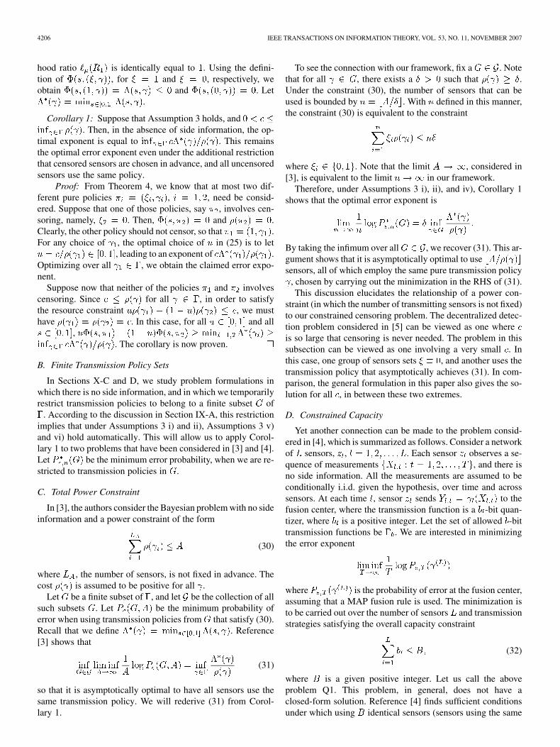
where each is a known spatial signal, andis Gaussian noise. When sensor sends its measurementto the fusion center, it consumes power (assumed posi-tive), which depends on its relative position to the fusion center.We constrain the overall average power to be less than a givenpositive constant . From Theorem 1, each sensor should usea common local censoring policy , obtained by max-imizing subject to .According to the discussion in Section VII, a sensor should becensored when is below a threshold. As a specificillustration, let and . Then

Suppose , where . (This is in line withstandard models used for power decay in a wireless network,see [12]. The unit cost is due to the power used to make themeasurement .) Then, we have

A specific case is shown in Fig. 1. We have taken , ,, and a constraint of . As shown, only sensors at

a large enough distance from the fusion center should transmittheir measurements .

IX. THE BAYESIAN PROBLEM WITH LOCAL CENSORING

We now consider the decentralized detection problem withcensoring in the Bayesian context. Let the prior probability of

be , for . We define andlet be the expectation operator with respect to (w.r.t.) . As inthe Neyman–Pearson case, we allow sensors to use randomizedsensor policies. In contrast to unconstrained Bayesian problems,simple examples show that randomization results in improvedperformance when the number of sensors is finite. However,


Fig. 1. The top graph shows the spatial signals plotted as a function of sensorlocation. Let c = 19=12. The bottom graph shows a plot of I(r)=�(r). A sensoris censored unless its location is in [�1;�0:5] or [0:5;1].

we will show that for the asymptotic problem considered here(no cooperation), randomization is unnecessary. In the process,we will also characterize the optimal error exponent and asso-ciated local policies.

A strategy is admissible if (1) is satisfied, with re-placing . For any admissible strategy , let de-note the resulting probability of error at the fusion center. Wewill always assume that the fusion center uses an optimal fu-sion rule, namely the maximum a posteriori probability (MAP)rule. Let be the infimum of over all admissiblestrategies. We are interested in finding asymptotically optimallocal strategies that achieve

Before we launch into the analysis, let us consider a simpleexample that shows that cooperation among the sensors isstrictly better than using local strategies.

Example 7: Suppose that the random variables belong to, are i.i.d. under either hypothesis, and that

, for . We assume that all sensorsare restricted to using the transmission function .

We assume that the distribution of under the two hy-potheses is the same when , but different when .Thus, it is only those sensors with that have usefulinformation to transmit. Under mild conditions (including thespecial case where has a finite range), it is a well-knownconsequence of the Chernoff bound that if exactly sensorshave and transmit to the fusion center, the probability oferror is of the form , where is a negative constantdetermined by the distributions of and where satisfies

. In particular, for every , we can

find some positive , , such that .Let and . Thus, the resource constraint

(1) becomes , where is the (random) number ofsensors that are not censored.

Assume for simplicity that is an integer. Consider thefollowing cooperative censoring strategy.

1) If , sensor transmits if only if .2) If , among those sensors with ,

arbitrarily choose of them to transmit.Using the Chernoff bound, we have forsome positive constant . Let be the probability of error atthe fusion center. We have

Suppose that when , the distribution of is such that, which is certainly possible. Since is arbitrary,

we obtain .Consider now a local and pure censoring strategy. In a best

strategy of this kind, every sensor with is censored, and. The only way to achieve this is as follows:

sensors are always censored; the remaining sensors are censoredif and only if . Thus, is binomial with parameters

and . After averaging over all possible values of , theprobability of error satisfies

Since is arbitrary, we obtain

This is strictly greater than , which shows that the coop-erative strategy constructed earlier has a better error exponent.Later on, we show that randomization cannot improve perfor-mance, bringing the conclusion that cooperative strategies canbe strictly better than local ones.

The essence of this example is that in the local case, we havemuch less control over the tails of the distribution of ; the pos-sibility of having a large deviation results in a deteriorationin the error exponent.


In general, optimal cooperative strategies are difficult tofind. As the cooperative strategy may also be practically infea-sible, we will focus our attention on finding an optimal localstrategy. For the remainder of this paper, the words “policy”and “strategy” will always mean “local policy” and “localstrategy,” respectively.

A. Notation and Assumptions

Let be the Radon–Nikodym derivative of the mea-sure w.r.t. . For , let bethe Radon–Nikodym derivative of the measure w.r.t.

. Let , and for any , andpure local transmission policy , let

Finally, for a randomized local policy , let

(23)

For a policy , if for alland , we will write . We will make thefollowing assumptions.

Assumption 3:i) Conditioned on either hypothesis, the random variables

are i.i.d. Furthermore, and are equivalent mea-sures.

ii) The (regular) conditional distributions andare equivalent for every .

iii) We are restricted to local strategies.iv) We have , for every and pure policy

.v) There exists an open interval ,

such that for all pure policies , we have. Furthermore, for

and , the following holds:

vi) For the same open interval as in v) above, there exists asuch that

and

for all and all .

Note that there is little loss of generality in imposing Assump-tion 3 iv). Indeed, if for some and some pure policy

, then we can always transmit when , without incur-ring any cost. So instead of censoring in the state , thesensor can always choose to transmit using this particular .

Assumptions 3 v) and vi) are required for the same tech-nical reasons as in [5], which also gives rather generalconditions under which they are satisfied.3 In general, theopen interval can be taken to be . Indeed, it canbe shown that, under Assumptions 3 i) and ii), and forany pure transmission policy , the minimizerof is in the interior of . If wetake , Assumption 3 v) reduces to the conditionthat the KL divergences and

are bounded. But we only needthe weaker version of Assumptions 3 v) and vi), as stated. Thisallows us to include cases where Assumptions 3 v) and vi)hold automatically. For example, if is a finite set of trans-mission policies, the interval only needs to include certain,finitely many, values of , and we can choose , where

. Then, it is easy to show that under Assumptions3 i) and ii), Assumptions 3 v)and vi) hold automatically. Wewill make use of this fact in Sections X-C and D. Another suf-ficient condition for Assumptions 3 v) and vi) are Assumptions3 i) and ii) together with an assumption similar to Assumption2 (see [5, Proposition 3]).

The main reason for introducing Assumption 3 is the fol-lowing lemma, which is proved in the Appendix.

Lemma 9: Suppose that Assumption 3 holds. Then, there ex-ists some such that for all and for all ,

, , and .

We record a result from [5], based on the results in [13], whichwill underlie the rest of our development. This result can also beobtained from [14, Theorem 1.3.13]. The result states that, if theconclusion of Lemma 9 holds, then

(24)

where stands for a term that vanishes as , uniformlyover all sequences . Given this result, we can just focus onthe problem of optimizing the RHS of (24), while ignoring the

term.

B. Optimal Strategy

In this subsection, we prove that asymptotic optimality can beobtained by dividing the sensors into two groups with sensorsin each group using a common pure policy.

Theorem 4: Under Assumption 3

(25)where the infimum is taken over all , and all purepolicies and that satisfy .

3Although [5] deals with the case of a finite transmission alphabet Y , theresults therein can be easily generalized to the case of infinite alphabets.


Proof: Fix some . Let be some (pos-sibly randomized) policies. Let be the pure policy obtainedwhen . Using the definition (23) of and Jensen’sinequality, we have

(26)

Similarly

Note that taking the average over all in the above expressionsis equivalent to taking an expectation over a uniformly chosenrandom . Let , where is chosen uniformly over

. We minimize the RHS of (26), , sub-ject to the constraint . Applying Lemma 8, with

and , we obtain

where the infimum is taken over all , and pure poli-cies , , satisfying the resource constraint

. Hence, from (24),

(27)To achieve the lower bound, suppose that and , ,

attain the infimum in (27) to within and that is aminimizing value of in (27). We assign sensors to usepolicy , and sensors to use policy . We censorany remaining sensor. Then, from (24)

and taking completes the proof.

Let us remark that similar results are easily obtained for thecase where the side information is not transmitted to the fusioncenter (cf. Section V-C).

C. Characterization of the Optimal Exponent

In this subsection and the next, we will consider the casewhere is finite, for two reasons. First, in many practical cases,because of the limited channel between each sensor and the fu-sion center, the side information can be assumed to take valuesfrom a finite alphabet. Second, when is finite, the analysis is

simplified and results in a simple form for the censoring policies.So without loss of generality, we will take .Let and .

Let us fix two pure local transmission policies and . Let

(28)

where the infimum is taken over all and pure cen-soring policies , that satisfy

From Theorem 4 and under Assumption 3, we have

(29)

Note that given and , the minimization in (28) has anoptimal solution. (This is because is finite, and thereforethere are only finitely many possible pure censoring policies.)Let be the value of in such an optimalsolution. It follows that must minimize (and,therefore, as well), subject to the constraint

. Note that isequal to

where .We can now give a characterization of the optimal , similar

to the one at the end of Section VII. For any , let

Proposition 3: Suppose Assumption 3 holds. Suppose thatis finite and that optimal choices of , , , have been fixed.Then, there exist thresholds , such that the correspondingoptimal censoring functions , satisfy the following: for each

, if , then , otherwise .

X. SPECIAL CASES AND EXAMPLES FOR THE

BAYESIAN PROBLEM

We now examine some special cases that will lead to simpli-fied versions of Theorem 4.

A. No Side Information

In this subsection, we consider the case of no side informa-tion, which is equivalent to having . Accordingly,will be suppressed from our notation below. For example, thecost incurred by a sensor making a measurement and transmit-ting it via a transmission function is denoted by .We will show that when in the resource constraint (1) is suf-ficiently small, we can restrict all uncensored sensors to use thesame policy.

Note that there are only two possible pure censoring policies,and . In the absence of side information, the likeli-


hood ratio is identically equal to . Using the defini-tion of , for and , respectively, weobtain and . Let

.

Corollary 1: Suppose that Assumption 3 holds, and. Then, in the absence of side information, the op-

timal exponent is equal to . This remainsthe optimal error exponent even under the additional restrictionthat censored sensors are chosen in advance, and all uncensoredsensors use the same policy.

Proof: From Theorem 4, we know that at most two dif-ferent pure policies , , need be consid-ered. Suppose that one of those policies, say , involves cen-soring, namely, . Then, and .Clearly, the other policy should not censor, so that .For any choice of , the optimal choice of in (25) is to let

, leading to an exponent of .Optimizing over all , we obtain the claimed error expo-nent.

Suppose now that neither of the policies and involvescensoring. Since for all , in order to satisfythe resource constraint , we musthave . In this case, for all and all

,. The corollary is now proven.

B. Finite Transmission Policy Sets

In Sections X-C and D, we study problem formulations inwhich there is no side information, and in which we temporarilyrestrict transmission policies to belong to a finite subset of

. According to the discussion in Section IX-A, this restrictionimplies that under Assumptions 3 i) and ii), Assumptions 3 v)and vi) hold automatically. This will allow us to apply Corol-lary 1 to two problems that have been considered in [3] and [4].Let be the minimum error probability, when we are re-stricted to transmission policies in .

C. Total Power Constraint

In [3], the authors consider the Bayesian problem with no sideinformation and a power constraint of the form

(30)

where , the number of sensors, is not fixed in advance. Thecost is assumed to be positive for all .

Let be a finite subset of , and let be the collection of allsuch subsets . Let be the minimum probability oferror when using transmission policies from that satisfy (30).Recall that we define . Reference[3] shows that

(31)

so that it is asymptotically optimal to have all sensors use thesame transmission policy. We will rederive (31) from Corol-lary 1.

To see the connection with our framework, fix a . Notethat for all , there exists a such that .Under the constraint (30), the number of sensors that can beused is bounded by . With defined in this manner,the constraint (30) is equivalent to the constraint

where . Note that the limit , considered in[3], is equivalent to the limit in our framework.

Therefore, under Assumptions 3 i), ii), and iv), Corollary 1shows that the optimal error exponent is

By taking the infimum over all , we recover (31). This ar-gument shows that it is asymptotically optimal to usesensors, all of which employ the same pure transmission policy

, chosen by carrying out the minimization in the RHS of (31).This discussion elucidates the relationship of a power con-

straint (in which the number of transmitting sensors is not fixed)to our constrained censoring problem. The decentralized detec-tion problem considered in [5] can be viewed as one whereis so large that censoring is never needed. The problem in thissubsection can be viewed as one involving a very small . Inthis case, one group of sensors sets , and another uses thetransmission policy that asymptotically achieves (31). In com-parison, the general formulation in this paper also gives the so-lution for all , in between these two extremes.

D. Constrained Capacity

Yet another connection can be made to the problem consid-ered in [4], which is summarized as follows. Consider a networkof sensors, , . Each sensor observes a se-quence of measurements , and there isno side information. All the measurements are assumed to beconditionally i.i.d. given the hypothesis, over time and acrosssensors. At each time , sensor sends to thefusion center, where the transmission function is a -bit quan-tizer, where is a positive integer. Let the set of allowed -bittransmission functions be . We are interested in minimizingthe error exponent

where is the probability of error at the fusion center,assuming that a MAP fusion rule is used. The minimization isto be carried out over the number of sensors and transmissionstrategies satisfying the overall capacity constraint

(32)

where is a given positive integer. Let us call the aboveproblem Q1. This problem, in general, does not have aclosed-form solution. Reference [4] finds sufficient conditionsunder which using identical sensors (sensors using the same


transmission policy), each sending one bit of information, isoptimal. We will apply our results to arrive at the same con-ditions as in [4], and also characterize the solution for specialvalues of .

As a first step, we will relax the constraints in problem Q1.We view each sensor over the time periods , as

different sensors , and hence remove the constraint thatall must use the same transmission policy . Because of(32), . Hence, we can imagine that we are starting with

sensors, some of which will be censored, and rewrite(32) as

(33)

where . For each for which isnonempty, consider a nonempty finite subset of , and use todenote the union of these subsets over . Let be the collectionof all such . With , we wish to minimize

We will obtain an optimal solution to the latter problem,which we call problem Q2. If from that optimal solution wecan derive a strategy that does not change the error exponentand yet meets the constraints that and forall , then we will have found an optimal solution to problemQ1. In particular, sufficient conditions for problem Q2 to haveall sensors using the same one-bit transmission policy are alsosufficient for problem Q1 to have identical one-bit sensors.

To put problem Q2 into our constrained censoring context,let for every , and note that . Let

. (If is empty, we set .)

Proposition 4: Suppose Assumptions 3 i) and ii) hold.i) For problem Q2,

In particular, using the same one-bit transmission func-tion at all uncensored sensors is asymptotically optimaliff .

ii) Let . For problem Q1, ifis an integer, we can restrict to using

sensors, all of them using the same -bit transmissionpolicy, without affecting the optimal exponent.

Proof: Part i) follows from Corollary 1. For part ii), letachieve to within . Let each of the sensors

in problem Q1 use . This comes within of the optimal ex-ponent for problem Q2, and therefore for problem Q1 as well.

Let , and note that

. Hence, for any

So if , we meet the sufficient conditions forproblem Q2 to achieve the optimal error exponent with iden-tical one-bit sensors. In that case, it is also optimal for problemQ1 to have identical one-bit sensors. This recovers Proposi-tion 2 of [4].

On the other hand, suppose that is an even integer and that. Then, it is strictly suboptimal to use identical

one-bit sensors for problem Q1. This is the content of [4, Propo-sition 3 ]. For a general that is not an integer multiple of , thesolution to Q1 involves an integer program, which can be diffi-cult to solve for large . However, as increases to infinity, wecan approach the optimal performance by using -bitsensors.

E. Independent of the Transmission Function

Suppose that for every value of the side information, all thetransmission functions in have the same cost, e.g., that theprocess of transmission under state requires the same energyfor all . Then, we can assume for some non-negative function . Suppose also that the set of transmissionpolicies is of the form , where is the setof allowed transmission policies , when the side informa-tion takes the value . Let

and

Corollary 2: Assume that for all ,and that Assumption 3 holds. Then

(34)where the infimum is taken over all and censoringpolicies that satisfy

Furthermore, it is optimal to use the same transmission policyfor all sensors.

Proof: The result is obtained from Theorem 4, by ob-serving that the constraints do not affect the optimization withrespect to and , and that

In this case, we use the same transmission policy at all sen-sors, and at most two different censoring policies. Suppose that

is a minimizing value of in (34). Then, for any , wecan use a transmission function that minimizes

, if the minimum is attained.

XI. CONCLUSION

We have formulated a general framework involving censoringin a sensor network, and resource constraints. We allow the sen-sors to censor based on some side information, while taking intoaccount a general cost function that depends only on the sideinformation and the transmission policy used by the sensor. Weallow the sensors to cooperate with each other and show that for


a Neyman–Pearson formulation, such cooperation is not nec-essary in the asymptotic regime of a large number of sensorsand small Type I error. Every sensor can independently use thesame (generally, randomized) local policy. An optimal policyis found by maximizing subject to theconstraint that . This maximizationcaptures the tradeoff between the Type II error exponent and theresource constraint.

In the Bayesian context, we have shown that, in the absenceof sensor cooperation, asymptotic optimality is obtained by di-viding the sensors into two groups, with every sensor in eachgroup using the same pure policy. We have also shown how tofind optimal strategies in some special cases, and the relation-ship of our results to other works.

Most of our results can be extended in various directions. Forexample, we may have multiple resource constraints. Withconstraints, we will generally need the local randomization vari-able to have a range of cardinality (Neyman–Pearsoncase), or to divide the sensors into groups, with everysensor in each group using the same policy (Bayesian case). Ex-tensions to the case of more than two hypotheses are also pos-sible, along the lines of [5].

APPENDIX

Proof of Lemma 8: Let

and

Clearly, . It remains to show that . Assume that, and fix an . Choose a such that

, and

(35)

Let be the convex hull of the set .It can be shown that the point

(see, for example, [15, p. 25]). Therefore, there exists a fi-nite set of points , and nonnegative scalars

summing to , such that

and

Consider the linear program in which we maximizeover the nonnegative scalars so

that and . From a well-knownresult in linear programming [11], there exists an optimalsolution to this linear program with at most two of thebeing nonzero. Hence, . From (35), we have

, and since is arbitrary, we obtain . The casewhere has a similar proof. The proof is now complete.

Proof of Lemma 9: For any fixed pure policy and a given, it is well known that the first and second

derivatives of , w.r.t. , are finite. What needs to beproved is that these derivatives are uniformly bounded for allpolicies .

For a given , let

(36)

so that . Then, for each ,

(37)

To prove the lemma, it suffices to show that for all policies andall , is uniformly bounded away from , andand are uniformly bounded. We do this in several stepsbelow. To keep the notation simple, we will abbreviate

to , to , and to .a) For every pure transmission policy , and every

and , we have , because, and is a convex

function of for each (see [7, Lemma 2.2.5]). There-fore, using Jensen’s inequality

(38)

Using the same technique as in the proof of Proposition 3of [5], we can show that , for all ,hence, . This implies that ,for all .

b) Let . Then, from (38), for all

It is easily shown that, and that both functions are convex in .

Then, for

(39)

(We used here the convexity of , which implies that themagnitude of its derivative is maximized at one of the end


points .) The finiteness of the RHS of (39) follows fromAssumption 3 v).

c) From b) above, for all . So, for thesame reason as in [7, Lemma 2.2.5 (c)], we can differen-tiate twice under the expectation operator. Hence,from (36), we have

from Assumption 3 vi).The steps above show that is uniformly bounded andcompletes the proof of the lemma.

ACKNOWLEDGMENT

We wish to thank the Associate Editor and the anonymous re-viewers for their suggestions and careful reading of the manu-script. We also wish to thank Prof. Devavrat Shah for his helpfulcomments.

REFERENCES

[1] C. Rago, P. Willett, and Y. Bar-Shalom, “Censoring sensors: Alow-communication-rate scheme for distributed detection,” IEEETrans. Aerosp. Electron. Syst., vol. 32, no. 2, pp. 554–568, Apr. 1996.

[2] S. Appadwedula, V. V. Veeravalli, and D. Jones, “Energy-efficient de-tection in sensor networks,” IEEE J. Sel. Areas Commun., vol. 23, no.4, pp. 693–702, Apr. 2005.

[3] J.-F. Chamberland and V. V. Veeravalli, “Asymptotic results for de-centralized detection in power constrained wireless sensor networks,”IEEE J. Select. Areas Commun., Special Issue on Wireless Sensor Net-works, vol. 22, no. 6, pp. 1007–1015, Jun. 2004.

[4] J.-F. Chamberland and V. V. Veeravalli, “Decentralized detection insensor networks,” IEEE Trans. Signal Process., vol. 51, no. 2, pp.407–416, Feb. 2003.

[5] J. N. Tsitsiklis, “Decentralized detection by a large number of sensors,”Math. Control, Signals, Syst., vol. 1, pp. 167–182, 1988.

[6] J. N. Tsitsiklis, “Decentralized detection,” Advances in StatisticalSignal Processing, vol. 2, pp. 297–344, 1993.

[7] A. Dembo and O. Zeitouni, Large Deviations Techniques and Applica-tions. New York: Springer-Verlag, 1998.

[8] R. E. Blahut, Principles and Practice of Information Theory.Reading, MA: Addison-Wesley, 1987.

[9] R. R. Bahadur, S. L. Zabell, and J. C. Gupta, “Large deviations, tests,and estimates,” in Asymptotic Theory of Statistical Tests and Estima-tion: In Honor of Wassily Hoeffding, I. M. Chakravarti, Ed. NewYork: Academic, 1980.

[10] R. Durrett, Probability: Theory and Examples, 2nd ed. New York,NY: Duxbury, 1995.

[11] D. Bertsimas and J. N. Tsitsiklis, Introduction to Linear Optimization,1st ed. Belmont, MA: Athena Scientific, 1997.

[12] D. N. C. Tse and P. Viswanath, Fundatmentals of Wireless Communi-cations. New York: Cambridge Univ. Press, 2005.

[13] C. E. Shannon, R. G. Gallager, and E. R. Berlekamp, “Lower boundsto error probability for coding on discrete memoryless channels, I,” Inf.Contr., vol. 10, pp. 65–103, 1967.

[14] D. Stroock, Probability Theory An Analytic View. Cambridge, U.K.:Cambridge Univ. Press, 1993.

[15] S. Boyd and L. Vandenberghe, Convex Optimization. Cambridge,U.K.: Cambridge Univ.Press, 2004.

Asymptotic Performance of a Censoring Sensor Network

Documents

Transcript of Asymptotic Performance of a Censoring Sensor Network