ASYMPTOTIC ANALYSIS OF THE SPECTRUM OF...

ASYMPTOTIC ANALYSIS OF THE SPECTRUM OF THE DISCRETE

HAMILTONIAN WITH PERIOD DOUBLING POTENTIAL

MEG FIELDS, TARA HUDSON, AND MARIA MARKOVICH

Abstract. The discrete Hamiltonian operator with period doubling potential is a pop-ular one-dimensional model of a quasi-crystal. The spectrum of this operator is a Cantorset for fixed coupling constants greater than zero. We numerically approximate this spec-trum using both matrix truncation and a trace map method. We then computationallyexamine the asymptotic behavior (i.e. as the coupling constant goes to zero) of thebox-counting dimension, thickness, and Hausdorff dimension for these approximations.

Contents

1. Introduction 12. The Period Doubling Hamiltonian 23. The Spectrum of the Operator 34. Box Counting Dimension 75. Thickness 86. Hausdorff Dimension 137. Future Work 178. Acknowledgements 17Appendix A. Code to Approximate the Spectrum 18Appendix B. Box Counting Dimension Code 26Appendix C. Thickness Code 30Appendix D. Hausdorff Dimension Code 39References 41

1. Introduction

The discovery of quasi-crystals in the 1980’s provoked many new questions in physicsand mathematics [1]. Quasi-crystals are materials that have some properties of crystals,specifically x-ray diffraction patterns, but have aperiodic lattices as opposed to the periodiclattices of crystals.

Date: August 1, 2013.This work was supported by NSF grant DMS-0739338.

1

2 MEG FIELDS, TARA HUDSON, AND MARIA MARKOVICH

Mathematically, we can model one-dimensional quasi-crystals using Hamiltonian oper-ators with aperiodic potentials [1], [2], [5]. The spectral properties of this operator corre-spond to physical attributes of the crystal. Particularly, fractal properties of such spectraaffect quantum diffusion patterns of electrons in quasi-crystalline materials [7], [4], [8].

In this paper, we examine the spectrum of the discrete Hamiltonian operator with perioddoubling potential. In Section 2, we describe the period doubling sequence and define theassociated operator. Section 3 gives two methods of approximating the spectrum of thisoperator. In Sections 4, 5, and 6 we give the mathematical definitions of three methods ofanalyzing fractal sets, that is, box-counting dimension, thickness, and Hausdorff dimension,respectively. In each section we explain the methods used.

Unfortunately, the trends in the data from the thickness computations were not con-sistent enough to be conclusive, but there were weak indications that thickness tends toinfinity as coupling constant goes to zero. Numerical experiments indicate both the box-counting and Hausdorff dimensions approach one as the coupling constant approaches zero.This result is consistent with what is known for other operators with aperiodic potentials(e.g. the Fibonacci Hamiltonian, as in [5]).

2. The Period Doubling Hamiltonian

2.1. The Period Doubling Sequence. The period doubling sequence is generated froma substitution rule on {A,B}. The substitution rule is given by

S : A 7→ AB S : B 7→ AAStarting with A, we have

S1(A) = A BS2(A) = A B A AS3(A) = A B A A A B A BS4(A) = A B A A A B A B A B A A A B A A.

Notice that after each successive iteration, the period of the sequence is twice that ofthe previous sequence. Iterating this substitution infinitely many times gives the infinitesequence. To obtain a sequence that is infinite in both directions, we reflect the sequenceacross the initial letter. We will use the period doubling sequence to define a discreteHamiltonian operator.

2.2. The Discrete Hamiltonian Operator. The Hamiltonian operator with period dou-bling potential, HV , is:

HV = −∆ + V̂ (1)

where ∆ is the discrete Laplacian of Z and V̂ is a multiplication operator. In particular, V̂inputs the period doubling sequence into the main diagonal of the Hamiltonian operator.The Hamiltonian operator will act on a sequence in `2(Z), see [2]

THE SPECTRUM OF THE HAMILTONIAN WITH PERIOD DOUBLING POTENTIAL 3

3. The Spectrum of the Operator

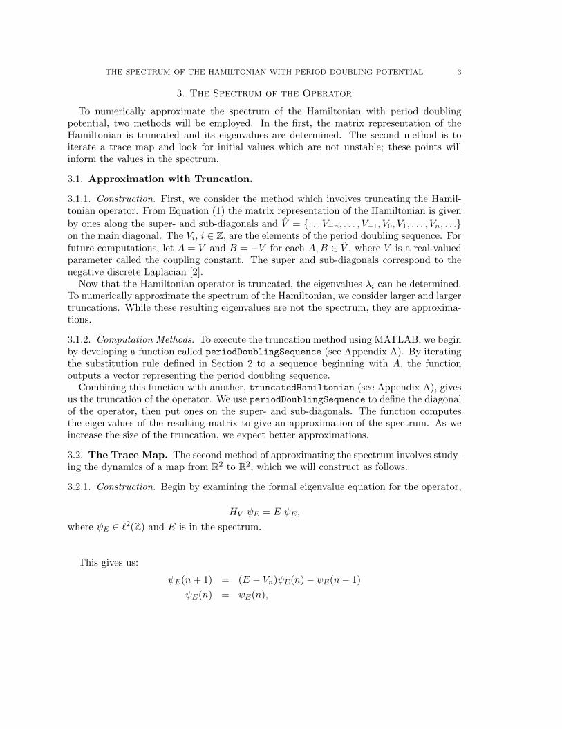
To numerically approximate the spectrum of the Hamiltonian with period doublingpotential, two methods will be employed. In the first, the matrix representation of theHamiltonian is truncated and its eigenvalues are determined. The second method is toiterate a trace map and look for initial values which are not unstable; these points willinform the values in the spectrum.

3.1. Approximation with Truncation.

3.1.1. Construction. First, we consider the method which involves truncating the Hamil-tonian operator. From Equation (1) the matrix representation of the Hamiltonian is given

by ones along the super- and sub-diagonals and V̂ = {. . . V−n, . . . , V−1, V0, V1, . . . , Vn, . . .}on the main diagonal. The Vi, i ∈ Z, are the elements of the period doubling sequence. Forfuture computations, let A = V and B = −V for each A,B ∈ V̂ , where V is a real-valuedparameter called the coupling constant. The super and sub-diagonals correspond to thenegative discrete Laplacian [2].

Now that the Hamiltonian operator is truncated, the eigenvalues λi can be determined.To numerically approximate the spectrum of the Hamiltonian, we consider larger and largertruncations. While these resulting eigenvalues are not the spectrum, they are approxima-tions.

3.1.2. Computation Methods. To execute the truncation method using MATLAB, we beginby developing a function called periodDoublingSequence (see Appendix A). By iteratingthe substitution rule defined in Section 2 to a sequence beginning with A, the functionoutputs a vector representing the period doubling sequence.

Combining this function with another, truncatedHamiltonian (see Appendix A), givesus the truncation of the operator. We use periodDoublingSequence to define the diagonalof the operator, then put ones on the super- and sub-diagonals. The function computesthe eigenvalues of the resulting matrix to give an approximation of the spectrum. As weincrease the size of the truncation, we expect better approximations.

3.2. The Trace Map. The second method of approximating the spectrum involves study-ing the dynamics of a map from R2 to R2, which we will construct as follows.

3.2.1. Construction. Begin by examining the formal eigenvalue equation for the operator,

HV ψE = E ψE ,

where ψE ∈ `2(Z) and E is in the spectrum.

This gives us:

ψE(n+ 1) = (E − Vn)ψE(n)− ψE(n− 1)

ψE(n) = ψE(n),


which can be represented as(ψE(n+ 1)ψE(n)

)=

((E − Vn)ψE(n)− ψE(n− 1)

ψE(n)

)=

(E − Vn −1

1 0

)(ψE(n)

ψE(n− 1)

).

Let

P (Vn, E) =

(E − Vn −1

1 0

)for Vn the nth entry of V̂ .

We now have the equation(ψE(n+ 1)ψE(n)

)= P (Vn, E)

(ψE(n)

ψE(n− 1)

), (2)

which we use to define the transfer matrix.

Definition 1. The matrix which describes the behavior of solutions to Equation (2), calledthe transfer matrix, is given by:

Tn =2n∏k=1

P (Vn, E).

For example, the transfer matrix for a single iteration of the sequence beginning withA = V is

T1 =2∏

k=1

[E − Vk −1

1 0

]=

[E − V1 −1

1 0

] [E − V2 −1

1 0

]=

[E − V −1

1 0

] [E + V −1

1 0

]=

[(E − V )(E + V )− 1 −(E − V )

(E + V ) −1

]Notice that

tr(T1) = (E − V )(E + V )− 2.

Now let A(n) and B(n) be the sequences starting with A = V and B = −V and generatedby n applications of the substitution rule. The transfer matrices corresponding to these

sequences are denoted by T(A)n and T

(B)n . Then

T(A)n+1 = T(B)

n T(A)n ,

T(B)n+1 = (T(A)

n )2.


This recursion in the transfer matrices can also be seen in their traces as follows. Definexn := tr(T

(A)n ) and yn := tr(T

(B)n ). Then we can verify that

xn+1 = tr(T(A)n+1) = xnyn − 2,

yn+1 = tr(T(B)n+1) = (xn)2 − 2.

This equation is the trace map. [2]

Example 2. To illustrate, we show the process for obtaining yn+1 of the map. Notewe make use of the fact that Tn is a uni-modular 2 × 2 matrix and thus satisfies T2

n =tr(Tn)Tn − I.

yn+1 = tr(T

(B)(n+1)

)= tr

(T

(AA)(n)

)= tr

((T

(A)(n)

)2)= tr

(tr(T

(A)(n)

)T

(A)(n) − I

)= tr

(tr(T

(A)(n)

)T(A)n

)− tr(I)

= xntr(T

(A)(n)

)− tr(I)

= x2n − 2.

The initial conditions for the trace map are x0 = E − V , y0 = E + V for some couplingconstant V .

We now explain how to find values in the spectrum of HV using the trace map.

Definition 3. Define a point (x, y) ∈ R2 to be unstable if x = x0 = E−V, y = y0 = E+V,and there is some N such that for all n > N , |xn| < 2.

To aid in determining which points are unstable, we can define a region A := {(x, y) | y >2 , |x| > 2}. Then the following holds:

Theorem 4 (Bellisard, Bovier, Ghez). A point (x, y) is unstable if and only if there existsn such that (xn, yn) ∈ A.

We denote the set of all unstable points to be U . The complement of this set will informthe spectrum by the following theorem.

Theorem 5. (Bellisard, Bovier, Ghez) E ∈ R is in the spectrum of HV if and only ifx = E − V and y = E + V are such that (x, y) ∈ Uc.

Finding all unstable points of the trace map will allow us to numerically approximatethe spectrum.


3.2.2. Computation Methods. The script traceMap (see Appendix A) allows us to approx-imate the complement of the set of unstable points, UC , as well as visualize this set alongwith the approximate spectrum. We iterate the trace map a number of times for an initialpoint (x0, y0) and then check the resulting values of x and y. If the points are not in theregion A = {(x, y) | y > 2, |x| > 2}, we store the initial point in an array. We can thenplot these points to visualize UC . We also calculate the possible E and V that definex0 = E − V and y0 = E + V not unstable. The values of E which define such points arein the spectrum, and we can plot them with the coupling constants.

−3 −2 −1 0 1 2 3−3

−2

−1

0

1

2

3

y

x

−2 −1.5 −1 −0.5 0 0.5 1 1.5 20

0.2

0.4

0.6

0.8

1

V

E

Student Version of MATLAB

Figure 1. Top: An approximation of UC . Bottom: An approximation ofthe spectrum.

3.3. Cantor Sets. The following theorem gives insight into the fractal nature of the spec-trum.

Theorem 6 (Bellisard, Bovier, Ghez). For a fixed coupling constant greater than zero, thespectrum of the Hamiltonian will be a Cantor set of Lebesgue measure zero.

Thus it is natural to ask questions about Hausdorff dimension, box-counting dimension,and thickness of the spectrum. We are particularly interested in the asymptotic behaviorof these measures as coupling constant approaches zero [5].


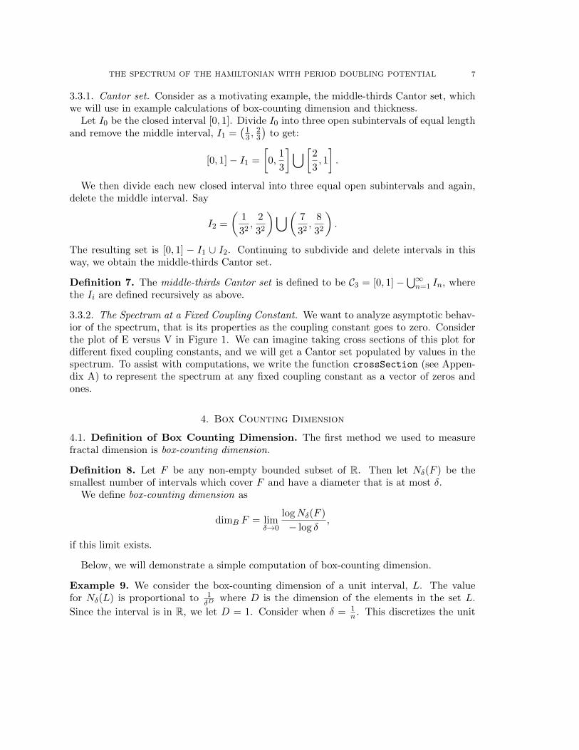
3.3.1. Cantor set. Consider as a motivating example, the middle-thirds Cantor set, whichwe will use in example calculations of box-counting dimension and thickness.

Let I0 be the closed interval [0, 1]. Divide I0 into three open subintervals of equal lengthand remove the middle interval, I1 =

(13 ,

23

)to get:

[0, 1]− I1 =

[0,

1

3

]⋃[2

3, 1

].

We then divide each new closed interval into three equal open subintervals and again,delete the middle interval. Say

I2 =

(1

32,

2

32

)⋃(7

32,

8

32

).

The resulting set is [0, 1] − I1 ∪ I2. Continuing to subdivide and delete intervals in thisway, we obtain the middle-thirds Cantor set.

Definition 7. The middle-thirds Cantor set is defined to be C3 = [0, 1]−⋃∞n=1 In, where

the Ii are defined recursively as above.

3.3.2. The Spectrum at a Fixed Coupling Constant. We want to analyze asymptotic behav-ior of the spectrum, that is its properties as the coupling constant goes to zero. Considerthe plot of E versus V in Figure 1. We can imagine taking cross sections of this plot fordifferent fixed coupling constants, and we will get a Cantor set populated by values in thespectrum. To assist with computations, we write the function crossSection (see Appen-dix A) to represent the spectrum at any fixed coupling constant as a vector of zeros andones.

4. Box Counting Dimension

4.1. Definition of Box Counting Dimension. The first method we used to measurefractal dimension is box-counting dimension.

Definition 8. Let F be any non-empty bounded subset of R. Then let Nδ(F ) be thesmallest number of intervals which cover F and have a diameter that is at most δ.

We define box-counting dimension as

dimB F = limδ→0

logNδ(F )

− log δ,

if this limit exists.

Below, we will demonstrate a simple computation of box-counting dimension.

Example 9. We consider the box-counting dimension of a unit interval, L. The valuefor Nδ(L) is proportional to 1

δDwhere D is the dimension of the elements in the set L.

Since the interval is in R, we let D = 1. Consider when δ = 1n . This discretizes the unit


interval into n partitions. Thus Nδ(L) = n. By inputting the results into the box-countingdimension equation we have:

dimB L = limδ→0

logNδ(L)

− log δ

= limn→∞

log n

− log 1n

= limn→∞

log n

log n− log 1= 1

Notice, that the limit changes from δ → 0 to n→∞. This is because we have defined δin terms of n.

Thus, the box-counting dimension of a unit interval is 1.

4.2. Computation Methods. The set we for which we approximate the box-countingdimension is the spectrum for a fixed coupling constant, represented by the vector generatedby the crossSection function. First, we use the function boxCountingDimension (seeAppendix B)to generate a number of different diameters, δ, using negative powers of two,then count the number of δ-covers needed to cover the cross section. Taking the ratio oflogarithms as in Definition 8 gives the approximate box-counting dimension for the set.

This function is now used to approximate the box-counting dimension of many sets withdifferent coupling constants approaching zero. The function bcdAsVtoZero (see Appen-dix B) runs boxCountingDimension for a number of exponentially decreasing couplingconstants.

4.3. Results. Several general trends were apparent in the numerical experiments withbox-counting dimension. In particular, as coupling constant approaches zero, the box-counting dimension approaches one. This is shown in Table 1, as well as graphically inFigure 2.

Thus, we conclude that as coupling constant approaches zero, box-counting dimen-sion approaches one. In similar mathematical quasi-crystals (in particular the FibonnacciHamiltonian), the box-counting and Hausdorff dimensions coincide [5]. Consider Figure 1.We notice that at coupling constant equal to zero, all values of E between −2 and 2 areincluded in the spectrum. It is known that for a coupling constant of zero, the spectrumis an interval in R and should have a box-counting dimension of one.

5. Thickness

5.1. Definition of Thickness. We will now consider the thickness of the spectrum.Let K ⊂ R be a Cantor set. Then we will define the gaps of K as follows.

Definition 10. A gap of K is a connected component of R\K. A bounded gap of K is abounded connected component of R\K.

To define thickness, we will consider bridges at the boundary points of the gaps.


Coupling Constant (V ) Box Counting Dimension0.02 0.67250.01 0.76100.005 0.85810.0025 0.91400.00125 0.95240.000625 0.97370.0003125 0.98230.00015625 0.98680.00007813 0.98950.00003906 0.99040.00001953 0.99110.00000977 0.9914

Table 1. The box-counting dimension as coupling constant approacheszero:

bcdAsVtoZero(0.4,−2.1, 2.1, 12, 1000)

0 0.001 0.002 0.003 0.004 0.005 0.006 0.007 0.008 0.009 0.010.75

0.8

0.85

0.9

0.95

1Box Counting Dimension as Coupling Constant Approaches Zero

Coupling Constant

Box

Cou

ntin

g D

imen

sion

Student Version of MATLAB

Figure 2. The effect of coupling constant on the box-counting dimension

Definition 11 ([9]). Let U be any bounded gap of K and u be a boundary point of U ,that is u ∈ K. Then a bridge of K at u, denoted C, is the maximal interval in R such that

• u is a boundary point of C, and


) (

13n

Figure 3. An interval of the nth iteration of the middle-thirds Cantor set.

) )( (

13n+1

13n+1

13n+1

uL uR

U

Figure 4. The line segment shown in Figure 3 after the subsequent iteration

• C contains no point of another gap, U ′ whose length, `(U ′) is at least the length U(where length is defined in the usual way for R).

Define the thickness of K at a particular u to be

τ(K,u) := `(C)\`(U).

We can now define the thickness of the entire set K.

Definition 12. The thickness of K, denoted τ(K), is the infimum over the τ(K,u) for allpoints u of bounded gaps.

Finding the thickness of the spectrum is useful because, in relation to Hausdorff dimen-sion, dimH, the thickness of a set, τ , defines a lower bound of the dimension.

Theorem 13. [9] If K ⊂ R is a Cantor set with thickness τ , then(log(2)

log(2 + 1τ )

)≤ dimH(K).

Example 14. To illustrate the calculation of thickness, we will determine the thickness ofthe middle-thirds Cantor set (C3).

Consider the nth iteration. At this point, we have intervals of length 13n and gaps with at

least this length. This is shown in Figure 3.After the next iteration, there are new gaps of length 1

3n+1 . Similarly the intervals are

all of length 13n+1 , as represented in Figure 4.

Thickness is given by:τ(C3) = inf(τ(C3, u)),


where

τ(C3, u) =l(C)

l(U)

such that l(C) is the length of the bridge and l(U) is the length of the gap. Consider uL,the left boundary point of the gap (U) in Figure 4. To calculate the thickness at uL, wewill generate a bridge starting at this point and ending at the boundary of a gap (Uk),where l(U) ≤ l(Uk).

Recall that every gap in the (n + 1)th iteration of C3 has length at least 13n+1 . There-

fore, the bridge will terminate at the next gap.

Thus,

l(C) =1

3n+1= l(U)

and hence,τ(C3, uL) = 1.

In a similar way, it can be shown that

τ(C3, uR) = 1.

Notice that uL and uR are arbitrary boundary points in C3, therefore,

τ(C3, u) = {1, ∀ boundary points u}.To calculate the thickness of C3, we will take the infimum of this set,

τ(C3) = inf(τ(C3, u)) = 1.

Therefore, the thickness of the middle-thirds Cantor set is 1.

5.2. Computation Methods. To approximate the thickness of the spectrum, we first usethe crossSection function (Appendix A) to represent the set. While approximating thick-ness, we ensure that this vector begins and ends in a string of zeros, which is accomplishedby allowing a larger range of input values than is necessary.

Recall Definition 12: to calculate thickness at a boundary point of a gap, we divide thelength of the bridge by the length of gap. We will numerically approximate this with severalMATLAB functions: intervalSize, gapSize and calculateThickness (see Appendix C).

In the binary representation of the spectrum, the zeros denote a gap while ones repre-sent an interval. In this way, we can count the number of consecutive zeros and ones toobtain the length of a gap and interval, respectively. Each quantity will be determinedusing the functions intervalSize and gapSize. In both functions, we consider each el-ement in the array generated by crossSection. For each consecutive one or zero, weincrease a counter variable by one. When the first different number is reached (zero or one,respectively), the magnitude of the counter is stored in a new array.

These two functions are then called upon to calculate the thickness for a given boundarypoint. This computation is completed in calculateThickness (see Appendix C).


In this function, we will determine the thicknesses for the right and left boundary points.In this process, we first choose a gap from the array obtained in gapSize. Recall that weensured the approximation of the spectrum would start and end with a gap. Thus, whenselecting a bounded gap, we ignore the first and last gaps. After the selection, we use thelengths of the gaps to find the first gap longer than or equal to the size of the chosen gap.The bridge will then travel to the right from the chosen boundary point to the longer gap.This bridge will extend over all gaps between the original and the ending gap, as well as theincluded intervals. To determine the length of the bridge, we add the appropriate entriesof the arrays obtained in gapSize and intervalSize.

Once the indices of the original and ending gaps have been determined, the sum of in-cluded gaps is a straightforward calculation. On the other hand, determining the lengthsof the included intervals is slightly more complicated. We notice that in general, theseintervals will have indices greater than or equal to that of the original gap, with one indexless than the that of the larger gap. The sum of these intervals are added to the sum ofthe gaps. The length of each bridge is stored in an array which is directly used to calculatethe thickness at each boundary point. To complete the calculation, we divide the lengthsof the corresponding bridges and gaps.

The thickness of the left boundary points are obtained by reflecting the vector of zerosand ones. We then take the thickness of the right boundary points for this reflected array.By definition, the overall thickness is the minimum of these values.

Finally, to analyze the thickness of the spectrum as the coupling constant approacheszero, we use the function plotThickness (see Appendix C). This function runs calculateThicknessfor a number of exponentially decreasing coupling constants and plots the resulting thick-nesses against the parameters.

5.3. Results. Overall, the computations indicate that as the coupling constant approacheszero, the thickness approaches infinity. Consider Table 2 which shows the result of thethickness calculation for the given coupling constant after 1,000 iterations of the tracemap.

Coupling Constant (V ) Thickness0.3 0.00370.03 0.01060.003 0.08330.0003 3.00.00003 383

Table 2. The thickness calculation as coupling constant approaches zero:calculateThickness(V,−3, 3, 210, 1000)

Notice that as the coupling constant approaches zero, the thickness approaches infinity.


When coupling constant is equal to zero, the spectrum is the closed interval [−2, 2]. Usingthe relation of thickness to Hausdorff dimension,

dimH(K) ≥ log(2)

log(2 + 1τ(K))

and the result,

limV→0

τ(K) =∞

it follows that at coupling constant zero,

limV→0

dimH(K) ≥ log(2)

log(2)= 1.

This is the expected dimension of an interval in R [9].

The result of the thickness approximation appears to be reasonable; however, we soonsee that the data obtained by the trace map does not allow for an accurate analysis. Byincreasing the number of iterations of the trace map, we obtain a more accurate represen-tation of the spectrum. However, the calculation of the thickness after a greater numberof iterations has a weaker asymptotic trend.

Table 3 shows the thicknesses and corresponding coupling constants obtained after 10,000iterations. Comparing these entries to those in Table 2, we see that for the same couplingconstants, the thickness that corresponds to the less accurate data grows more quickly.This indicates that the trend of thickness is not strong enough to form conclusions.

Coupling Constant (V ) Thickness0.03 0.01160.003 0.01250.0003 0.09090.00003 10.000003 17

Table 3. The thickness calculation as coupling constant approaches zero:calculateThickness(V,−3, 3, 210, 10000)

For these reasons, we take note of the thickness of the approximated spectrum, but focusmore on the box-counting dimension and Hausdorff dimension.

6. Hausdorff Dimension

6.1. Definition of Hausdorff Dimension. Finally, we consider the Hausdorff dimensionof the spectrum.

To calculate the Hausdorff dimension, we consider the covers of a set, U .


Definition 15. The diameter of the cover, |U |, is given by,

|U | = sup{|x− y| : x, y ∈ U}

To find the Hausdorff measure, consider the covers with diameter at most δ, and takethe limit as δ approaches zero.

Definition 16.

Hs(F ) = limδ→0

(inf

{ ∞∑i=1

|Ui|s : {Ui} is a δ cover

})This can be verified using the following theorem and proof.

Theorem 17. For a fixed δ < 1, Hsδ(F ) is non-increasing with respect to s.

Proof, from [6]. We want to show:

If s < t then Hsδ(F ) ≥ Htδ(F )

Let {Ui} be a δ cover of F. Then,∑|Ui|s ≥

∑|Ui|t

inf∑|Ui|s ≥ inf

∑|Ui|t

Now consider∑|Ui|t: ∑

|Ui|t ≤∑|Ui|t−s|Ui|s

≤ δt−s∑|Ui|s

Incorporating Hausdorff measure, it follows that:

Htδ(F ) ≤ δt−sHsδ(F ).

Letting Hsδ(F ) <∞ and δ approach 0 we have:

Ht(F )→ 0.

Next, if we let Htδ(F ) > 0 and δ approach 0, we have:

Hs(F )→∞.

�

Thus, the Hausdorff dimension is defined as follows.

Definition 18. Let F ⊂ Rn, F 6= ∅, s > 0 a real number. Then the Hausdorff dimensionof F is

dimH(F ) = inf {s ≥ 0 : Hs(F ) = 0} = sup {s : Hs(F ) =∞}


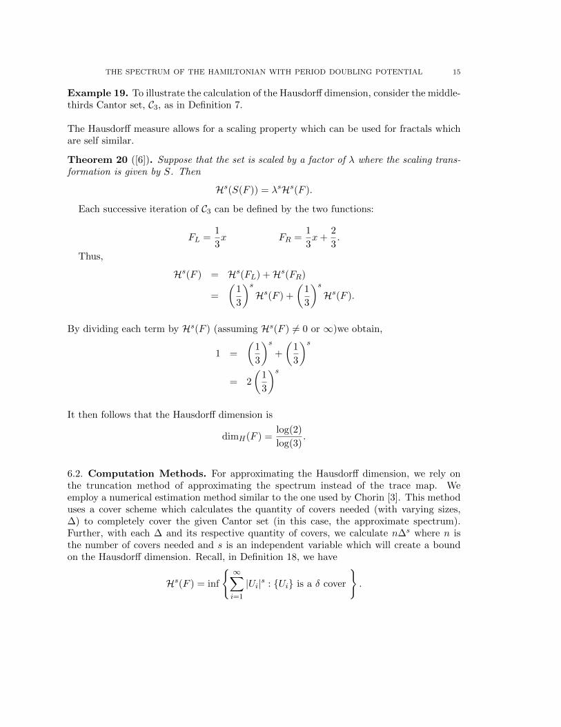
Example 19. To illustrate the calculation of the Hausdorff dimension, consider the middle-thirds Cantor set, C3, as in Definition 7.

The Hausdorff measure allows for a scaling property which can be used for fractals whichare self similar.

Theorem 20 ([6]). Suppose that the set is scaled by a factor of λ where the scaling trans-formation is given by S. Then

Hs(S(F )) = λsHs(F ).

Each successive iteration of C3 can be defined by the two functions:

FL =1

3x FR =

1

3x+

2

3.

Thus,

Hs(F ) = Hs(FL) +Hs(FR)

=

(1

3

)sHs(F ) +

(1

3

)sHs(F ).

By dividing each term by Hs(F ) (assuming Hs(F ) 6= 0 or ∞)we obtain,

1 =

(1

3

)s+

(1

3

)s= 2

(1

3

)sIt then follows that the Hausdorff dimension is

dimH(F ) =log(2)

log(3).

6.2. Computation Methods. For approximating the Hausdorff dimension, we rely onthe truncation method of approximating the spectrum instead of the trace map. Weemploy a numerical estimation method similar to the one used by Chorin [3]. This methoduses a cover scheme which calculates the quantity of covers needed (with varying sizes,∆) to completely cover the given Cantor set (in this case, the approximate spectrum).Further, with each ∆ and its respective quantity of covers, we calculate n∆s where n isthe number of covers needed and s is an independent variable which will create a boundon the Hausdorff dimension. Recall, in Definition 18, we have

Hs(F ) = inf

{ ∞∑i=1

|Ui|s : {Ui} is a δ cover

}.


The function, hausdorffDimension (see Appendix D), calls on truncatedHamiltonian

to obtain the eigenvalues of the truncated Hamiltonian, then numerically estimates theHausdorff dimension using the approach outlined above.

6.3. Results. The following tables represent the results from the equation n∆s with vary-ing coupling constants. Examining the s values gives insight into the Hausdorff dimensionof the spectrum. When s < dimH F we expect the values of n∆s to increase. Alterna-tively if s > dimH F , we hope to see the values of n∆s decrease. Thus we can estimate alower and upper bound on Hausdorff dimension, respectively, using the s values with thesecharacteristics [3].

Each row in the following tables denotes ∆ = 2−i.

si 0.85 0.90 0.95 1.0 1.05 1.1

1 4.993 4.823 4.659 4.500 4.347 4.1992 5.232 4.882 4.555 4.250 3.965 3.7003 5.635 5.078 4.577 3.875 3.373 2.9374 5.873 5.113 4.451 3.875 3.373 2.9375 6.096 5.127 4.311 3.625 3.048 2.5636 6.356 5.163 4.194 3.406 2.767 2.2477 6.567 5.153 4.043 3.172 2.489 1.9538 6.479 4.910 3.721 2.820 2.137 1.620

Table 4. Coupling Constant of 0.2

Note that the lower bound on Hausdorff dimension in Table 4 is s = .90. The upperbound is found at s = 1.

si 0.80 0.85 0.90 0.95 1.0 1.05 1.1

1 5.169 4.993 4.823 4.659 4.50 4.347 4.1992 5.608 5.232 4.882 4.555 4.250 3.965 3.7003 6.252 5.635 5.078 4.577 4.125 3.718 3.3514 7.073 6.158 5.361 4.667 4.063 3.537 3.0795 8.063 6.780 5.701 4.794 4.031 3.390 2.8516 9.225 7.493 6.087 4.944 4.016 3.262 2.6497 10.556 8.282 6.498 5.098 4.000 3.138 2.4628 11.972 9.073 6.876 5.211 3.949 2.993 2.268



The lower and upper bound on Hausdorff dimension in Table 5 is the same as that inTable 4 above.

si 0.92 0.93 0.94 0.95 0.96 0.97 0.98 0.99 1.00

1 4.757 4.724 4.691 4.659 4.627 4.595 4.563 4.531 4.5002 4.748 4.683 4.619 4.555 4.492 4.430 4.369 4.309 4.2503 4.872 4.771 4.673 4.577 4.483 4.391 4.300 4.212 4.1254 5.071 4.933 4.798 4.667 4.539 4.415 4.294 4.177 4.0635 5.319 5.138 4.963 4.794 4.631 4.473 4.321 4.173 4.0316 5.601 5.373 5.154 4.944 4.742 4.549 4.364 4.186 4.0167 5.909 5.629 5.362 5.108 4.866 4.636 4.416 4.207 4.0088 6.239 5.903 5.584 5.283 4.998 4.729 4.474 4.232 4.004


Notice that the lower bound on Hausdorff dimension in Table 6 is s = 0.92. The upperbound is at s = 1.00.

So we conclude that as the coupling constant approaches zero, the Hausdorff dimensionof the spectrum approaches one.

7. Future Work

Further work for this problem includes refining the approximations of the two fractaldimensions, refining the approach to the thickness computations, and analyzing the physicalimplications of the results.

8. Acknowledgements

We would like to thank our advisor, May Mei, and our project TA, Drew Zemke. Thanksalso to Ravi Ramakrishna, Summer Math Institute program director, and the math de-partment at Cornell University.


Appendix A. Code to Approximate the Spectrum

1 f unc t i on [ sequence ] = per iodDoubl ingSequence (n)

% periodDoubl ingSequence gene ra t e s the f i r s t n i t e r a t i o n s o f the per iod

3 % doubl ing sequence .

%

5 % Created By : Meg Fie lds , Tara Hudson , Maria Markovich

%

7 % INPUT:

% n = The number o f i t e r a t i o n s o f the per iod doubl ing sequence

9 % OUTPUT:

% sequence = An array o f the per iod doubl ing sequence a f t e r n

11 % i t e r a t i o n s

13

% For computat ional purposes , d e f i n e numeric va lue s f o r the e lements in the

15 % per iod doubl ing sequence .

A = 1 ;

17 B= −1;

19 %An array to hold the (n−1)th sequence , used to generate the subsequent

%i t e r a t i o n . Begin with A.

21 sequence = [A ] ;

23 % I t e r a t e the sequence n t imes .

f o r j = 1 : n

25

% An array in which to bu i ld the cur rent i t e r a t i o n o f the per iod

27 % doubl ing sequence .

cur r ent = [ ] ;

29

% Consider e lements o f the sequence a f t e r the prev ious i t e r a t i o n .

31 f o r i = 1 : l ength ( sequence ) ;

33 % I f the element i s an A, put ( A B ) at the end o f the ’ s torage ’

% array .

35 i f sequence ( i ) == A

37 cur rent ( l ength ( cur rent ) + 1 ) = A;

39 cur rent ( l ength ( cur rent ) + 1 ) = B;

41 % Simi l a r l y , i f the element i s a B, put ( A A) at the end o f the

% sto rage array .

43 e l s e i f sequence ( i ) == B


45 cur rent ( l ength ( cur rent ) + 1)= A;

47 cur rent ( l ength ( cur rent ) + 1) = A;

49 end

51 end

53 end

55 % Before the next i t e r a t i o n , r e d e f i n e the ’ sequence ’ to be the s to rage

% array .

57 sequence = current ;

59 end


f unc t i on [ e i g e n v a l u e s ] = truncatedHamiltonian (n , V)

2 % truncatedHamiltonian r e tu rn s the e i g e n v a l u e s o f a truncated Hamiltonian

% operator with per iod doubl ing p o t e n t i a l .

4 %

% Created By : Meg Fie lds , Tara Hudson , Maria Markovich

6 %

% INPUT:

8 % n = how many times the sequence i s i t e r a t e d V = coup l ing constant

% OUTPUT:

10 % e i g e n v a l u e s = the e i g e n v l a u e s o f the truncated hami ltonian

% operator .

12

14 % Fir s t , use the per iodDoubl ingSequence func t i on to generate the main

% diagona l o f the truncated matrix .

16 sequence = per iodDoubl ingSequence ( n ) ;

18 % R e f l e c t the r e s u l t over the s t a r t i n g po int to obta in the sequence in the

% negat ive d i r e c t i o n (” negat ive i t e r a t i o n s ”) . R e f l e c t i o n i s a property o f

20 % the per iod doubl ing sequence .

22 % Put both sequence and and i t s r e f l e c t i o n along the main d iagona l o f the

% matrix .

24 d iagona l = [ f l i p l r ( sequence ) sequence ] ;

26 % The truncated Hamiltonian operator w i l l have one ’ s a long the super and

% sub−d iagona l s . Mult ip ly the main d iagona l by the coup l ing constant to get

28 % the d e s i r e d p o t e n t i a l .

30 hami ltonian = diag ( V ∗ d iagona l ) + diag ( ones ( l ength ( d iagona l ) − 1 , 1 ) ,

1 ) . . .

+ diag ( ones ( l ength ( d iagona l ) − 1 , 1 ) , −1 ) ;

32

34 %Calcu la t e the e i g e n v a l u e s o f the truncated Hamiltonian operator . These

%va lues approximate the spectrum .

36 e i g e n v a l u e s = e i g ( hami l tonian ) ;

38 end


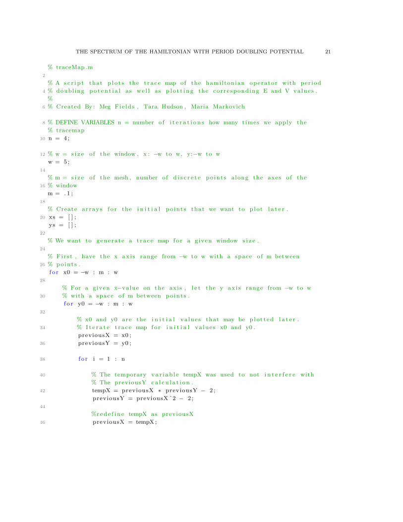
% traceMap .m

2

% A s c r i p t that p l o t s the t r a c e map o f the hami l tonian operator with per iod

4 % doubl ing p o t e n t i a l as we l l as p l o t t i n g the corre spond ing E and V va lues .

%

6 % Created By : Meg Fie lds , Tara Hudson , Maria Markovich

8 % DEFINE VARIABLES n = number o f i t e r a t i o n s how many times we apply the

% tracemap

10 n = 4 ;

12 % w = s i z e o f the window , x : −w to w, y:−w to w

w = 5 ;

14

% m = s i z e o f the mesh , number o f d i s c r e t e po in t s a long the axes o f the

16 % window

m = . 1 ;

18

% Create ar rays f o r the i n i t i a l po in t s that we want to p l o t l a t e r .

20 xs = [ ] ;

ys = [ ] ;

22

% We want to generate a t r a c e map f o r a g iven window s i z e .

24

% Fir s t , have the x a x i s range from −w to w with a space o f m between

26 % po int s .

f o r x0 = −w : m : w

28

% For a given x−value on the axis , l e t the y a x i s range from −w to w

30 % with a space o f m between po in t s .

f o r y0 = −w : m : w

32

% x0 and y0 are the i n i t i a l va lue s that may be p lo t t ed l a t e r .

34 % I t e r a t e t r a c e map f o r i n i t i a l va lue s x0 and y0 .

previousX = x0 ;

36 previousY = y0 ;

38 f o r i = 1 : n

40 % The temporary v a r i a b l e tempX was used to not i n t e r f e r e with

% The previousY c a l c u l a t i o n .

42 tempX = previousX ∗ previousY − 2 ;

previousY = previousX ˆ2 − 2 ;

44

%r e d e f i n e tempX as previousX

46 previousX = tempX ;


48 end

50 % We want to only look at the i n i t i a l va lue s where ” previousX ”

% never has an abso lu t e va lue g r e a t e r than 2 and where ” previousY ”

52 % i s never g r e a t e r than 2 . These are the ”not unstab le ” po in t s o f

% the t r a c e map .

54

i f not ( abs ( previousX )> 2 && previousY > 2)

56

% I f a value s a t i s f i e s the se cond i t i ons , put the i n i t i a l va lue in

58 % the array to p l o t l a t e r .

60 xs ( l ength ( xs ) + 1 ) = x0 ;

ys ( l ength ( ys ) + 1 ) = y0 ;

62

end

64

end

66

end

68

% Calcu la t e the E and V va lues from the i n i t i a l va lue o f x and y .

70 Es = ( xs + ys ) / 2 ;

Vs = ( −xs + ys ) / 2 ;

72

74 % Plot the po in t s :

76 % xs i s the l i s t o f i n i t i a l va lue s o f x that work

% ys i s the l i s t o f i n i t i a l va lue s o f y that work

78 f i g u r e ;

subplot ( 211 )

80 p lo t ( xs , ys , ’ b . ’ )

y l a b e l ( ’ y ’ )

82 x l a b e l ( ’ x ’ )

84 % plo t the E and V va lues

subplot ( 212 )

86

% We only want p o s i t i v e V va lues thus the a x i s c o n d i t i o n s .

88 p lo t ( Es , Vs , ’ g . ’ )

a x i s ( [−3 3 0 3 ] )

90 y l a b e l ( ’V ’ )

x l a b e l ( ’E ’ )


1

f unc t i on [ Es ] = c r o s s S e c t i o n ( V, Emin , Emax, k , n )

3

%c r o s s S e c t i o n prov ides a r e p r e s e n t a t i o n o f va lue s in the spectrum , E’ s , f o r

5 %a p a r t i c u l a r coup l ing constant V.

%

7 % Created by : Meg Fie lds , Tara Hudson , and Maria Markovich .

%

9 % INPUT: V = coup l ing contant , a r e a l va lue between 0 and 1

% Emin/max = the f i r s t and l a s t va lue s to con s id e r f o r the spectrum

11 % k = the number o f E va lue s in between the f i r s t and l a s t to

con s id e r

% n = number o f i t e r a t i o n s o f the t r a c e map

13 % OUTPUT: Es = a ” c r o s s s e c t i o n ” o f the spectrum

15 %Make a vec to r o f E−va lue s to check f o r ” in or out o f spectrum”

Evals = l i n s p a c e ( Emin , Emax, k ) ;

17

%Make a blank vec to r o f the same length as E−va lue s . By the end , t h i s w i l l

19 %have 0 s cor re spond ing to E−va lue s ”out o f spectrum” and 1 s f o r ” in the

spectrum . ”

Es = ze ro s ( 1 , k ) ;

21

23 %Star t with the f i r s t E−value in Evals , r epeat t i l we reach the end .

f o r j = 1 : k

25

27 %Def ine the i n i t i a l po in t s in terms o f the f i x e d coup l ing constant V

%and the p a r t i c u l a r E−value we ’ re l ook ing at t h i s round .

29 i n i t i a l x = Evals ( j ) − V;

i n i t i a l y = Evals ( j ) + V;

31

prev iousx = i n i t i a l x ;

33 prev iousy = i n i t i a l y ;

35 %I t e r a t e the t r a c e map f (x , y ) = ( ( xy − 2) , ( xˆ2 − 2) ) n t imes .

f o r i = 1 : n

37

tempx = ( prev iousx ∗ prev iousy ) − 2 ;

39 prev iousy = ( prev iousx ) ˆ2 − 2 ;

41 prev iousx = tempx ;

43 end


45 %Check the ” unstab le ” c o n d i t i o n s . I f the i n i t i a l po int i s unstable ,

%the E−value we used i s ” out o f spectrum , ” i . e . 0 . I f the i n i t i a l

po int i s

47 %not unstable , the E−value i s ” in spectrum , ” i . e . 1 .

49 Es ( j ) = not ( abs ( prev iousx )> 2 && prev iousy > 2) ;

51 end

53 end


Appendix B. Box Counting Dimension Code

f unc t i on [ dimensionV ] = boxCountingDimension ( V, Emin , Emax, k , n )

2

%boxCountingDimension approximates the box−count ing dimension o f the

4 %spectrum at a p a r t i c u l a r coup l ing constant .

%

6 % Created by : Meg Fie lds , Tara Hudson , and Maria Markovich .

%

8 % INPUT: V = coup l ing contant , a r e a l va lue between 0 and 1 .

% Emin/max = the f i r s t and l a s t va lue s to con s id e r f o r the

10 % spectrum .

% k = the power o f 2 to inform the number o f E va lue s in between

12 % the f i r s t and l a s t to con s id e r .

% n = number o f i t e r a t i o n s o f the t r a c e map .

14 % OUTPUT: dimensionV = the approximated dimension o f the specrum .

16

%Es i s a ” c r o s s s e c t i o n ” o f the spectrum f o r a p a r t i c u l a r coup l ing

18 %constant . I t i s an i n t e r v a l f i l l with 0 s and 1s , with 1 s r e p r e s e n t i n g the

%p o s i t i o n o f v a l e s in the spectrum .

20

%Note , The l ength o f t h i s vec to r needs to be a power o f two .

22

Es = c r o s s S e c t i o n ( V, Emin , Emax, 2ˆk , n ) ;

24

%Since we ’ l l choose an i n t e r v a l wider than what we expect to a c t u a l l y conta in

26 %the spectrum , we should make sure that the endpoints are 0 .

i f not ( Es (1 ) == 0 )

28 e r r o r ( ’ i nac cu ra t e data ’ )

end

30

i f not ( Es (2ˆ k ) == 0 )

32 e r r o r ( ’ i nac cu ra t e data ’ )

end

34

%Empty v ec to r s to hold the de l t a va lue s and the number o f d e l t a cover s .

36 d e l t a s = [ ] ;

Ndeltas = [ ] ;

38

f o r i = 1 : k

40

%Def ine each new d e l t a to be a negat ive power o f two .

42

d e l t a = 2ˆ(− i ) ;

44 d e l t a s ( i ) = d e l t a ;


cover = 0 ;

46

48 %Star t check ing th ing s at the beg inning o f the i n t e r v a l .

s t a r t = 1 ;

50

%While we s t i l l have more in the i n t e r v a l to check .

52 whi le s t a r t < l ength ( Es )

54 f o r check = s t a r t : l ength ( Es )

56 i f Es ( check ) == 1

58 %add one to the cover count , jump ahead in the i n t e r v a l by the

%length o f the cover .

60 cover = cover + 1 ;

s t a r t = check + length ( Es ) / 2ˆ i ;

62

%Stop check ing .

64 break ;

end

66

68 end

70 %Stop when we run out o f th ing s to check .

i f check == length ( Es )

72 break ;

end

74

76 end

%Put the number o f cover s f o r t h i s d e l t a in the Ndeltas vec to r .

78 Ndeltas ( l ength ( Ndeltas ) + 1 ) = cover ;

80 end

82

%Time to c a l c u l a t e the dimension f o r t h i s coup l ing constant !

84

%Plot po in t s in the plane where (x , y ) = (− l og ( d e l t a ) , l og ( Ndelta ) ) .

86 xAxis = −l og ( d e l t a s ) ; yAxis = log ( Ndeltas ) ;

88 %Find the best f i t l i n e o f the po in t s .

be s tF i tL ine = p o l y f i t ( xAxis , yAxis , 1 ) ;

90


%The s l ope o f t h i s l i n e i s the box−count ing dimension o f the spectrum at

92 %t h i s coup l ing constant !

dimensionV = bes tF i tL ine (1 ) ;

94

96 end


f unc t i on [ dimensionsAsVtoZero ] = bcdAsVtoZero ( Vinput , Emin , Emax, k , n )

2

%bcdAsVtoZero c r e a t e s a ta b l e o f the box−count ing dimensions with t h e i r

4 %r e s p e c t i v e coup l ing cons tant s . We w i l l be l ook ing at coup l ing cons tant s

%going to 0 .

6

% Created by : Meg Fie lds , Tara Hudson , and Maria Markovich .

8

% INPUT: −Vinput = the f i r s t ( and l a r g e s t ) coup l ing constant at which to

10 % c a l c u l a t e box−count ing dimension .

% −Emin/max = the f i r s t and l a s t va lue s to con s id e r f o r the

12 % spectrum .

% −k = the power o f 2 to inform the number o f E va lue s in between

14 % the f i r s t and l a s t to con s id e r .

% −n = number o f i t e r a t i o n s o f the t r a c e map .

16 % OUTPUT: demensionsAsVtoZero = a ta b l e with V, dimension V.

18 %Vectors to hold each new V and dimension .

Vs = ze ro s ( 1 , k ) ;

20 dimensions = ze ro s ( 1 , k ) ;

22

%For loop to c a l c u l a t e the box−count ing dimension at e x p o n e n t i a l l y

24 %dec r ea s ing Vs .

f o r j = 1 : k

26

Vnext = 2ˆ(− j ) ∗ Vinput ;

28

%Use the boxCountingDimension func t i on to f i n d the dimension at t h i s V.

30 dimensionV = boxCountingDimension ( Vnext , Emin , Emax, k , n ) ;

32 %Put the va lue s we ’ ve used in the appropr ia t e v e c t o r s .

Vs( j ) = Vnext ;

34 dimensions ( j ) = dimensionV ;

36

end

38

%Make a t ab l e o f Vs with t h e i r dimensions .

40 dimensionsAsVtoZero = [ Vs ; dimensions ] ’ ;

42

end


Appendix C. Thickness Code

f unc t i on [ gaps ] = gapSize ( Es )

2 % gapSize counts the l ength o f gaps in a cantor s e t r ep re s ented by a vec to r

% o f 0 ’ s and 1 ’ s .

4 %

% Created by : Meg Fie lds , Tara Hudson , Maria Markovich

6 %

% INPUT:

8 % Es = a sequence o f 0 ’ s and 1 ’ s where 0 ’ s r ep r e s e n t gaps and 1 ’ s

% r ep r e s e n t po in t s in the cantor s e t . Use the c r o s s S e c t i o n func t i on to

10 % generate t h i s .

% OUTPUT:

12 % gaps = The numbers o f con s e cu t i v e 0 s found thoughout Es .

14

% The number o f 0 ’ s w i l l be counted . F i r s t s e t t h i s v a r i a b l e to zero .

16 numzeros = 0 ;

18 % An array to s t o r e the l eng th s o f the runs o f 0 ’ s .

gaps = [ ] ;

20

% Star t l ook ing through the sequence l ook ing f o r 0 ’ s . Once a 0 i s found ,

22 % the counter w i l l i n c r e a s e by one .

f o r i = 1 : l ength ( Es )

24

i f Es ( i ) == 0

26

numzeros = numzeros + 1 ;

28

30 % I f in s t ead there i s a one in t h i s po s i t i on , put the number o f

% one ’ s in the array and then s e t the counter back to zero .

32 e l s e

34 %I f we haven ’ t counted any ones , we don ’ t want to put 0 in the

%s i z e s vec to r .

36 i f numzeros ˜= 0

38 gaps ( l ength ( gaps ) + 1 ) = numzeros ;

40 numzeros = 0 ;

42 end

44 end


46 end

48 % We need a s p e c i a l case f o r those sequences that end in a zero . In these

% sequences the counter w i l l not record the appropr ia t e va lue without an

50 % a d d i t i o n a l c o n d i t i o n a l statement .

i f Es ( l ength ( Es ) ) == 0

52

gaps ( l ength ( gaps ) + 1 ) = numzeros ;

54

56 end


2 f unc t i on [ s i z e s ] = i n t e r v a l S i z e ( Es )

% i n t e r v a l S i z e i s a func t i on that counts the l ength o f cons e cu t i v e 1 ’ s in a

4 % vector o f 0 ’ s and 1 ’ s

%

6 % Created by : Meg Fie lds , Tara Hudson , Maria Markovich

8 % INPUT:

% Es = a sequence o f 0 ’ s and 1 ’ s . Use the c r o s s S e c t i o n func t i on to

10 % generate t h i s .

% OUTPUT:

12 % s i z e s = The numbers o f the cons e cu t i v e 1 ’ s found thoughout Es .

14

% The number o f 1 ’ s w i l l be counted . F i r s t s e t t h i s v a r i a b l e equal to zero .

16 numones = 0 ;

18 % At array to s t o r e the l eng th s o f the runs o f 1 ’ s .

s i z e s = [ ] ;

20

%Star t l ook ing through the sequence to f i n d 1 ’ s . Once a 1 i s found ,

22 % the counter w i l l i n c r e a s e by one .

f o r i = 1 : l ength ( Es )

24

26 i f Es ( i ) == 1

numones = numones + 1 ;

28

30 % I f in s t ead there i s a zero in t h i s po s i t i on , put the cur rent

% count o f 1 ’ s in ’ s i z e s ’ , then s e t the counter back to zero .

32 e l s e

34 %I f we haven ’ t counted any ones , we don ’ t want to put 0 in the

%s i z e s vec to r .

36 i f numones ˜= 0

38 s i z e s ( l ength ( s i z e s ) + 1 ) = numones ;

40 numones = 0 ;

42 end

44 end

46 end


48 % We need a s p e c i a l case f o r those sequences that end in a one . In these

% sequences the counter w i l l not record the appropr ia t e va lue without an

50 % a d d i t i o n a l c o n d i t i o n a l statement .

i f Es ( l ength ( Es ) ) == 1

52

s i z e s ( l ength ( s i z e s ) + 1 ) = numones ;

54

end


f unc t i on [ th icknessmin ] = c a l c u l a t e T h i c k n e s s ( Es )

2 % c a l c u l a t e t h i c k n e s s approximates the t h i c k n e s s o f a cantor s e t r ep re s ented

% by a vec to r o f 0 ’ s and 1 ’ s (1 = point in the s e t ; 0 = gap ) .

4 %

% Created by : Meg Fie lds , Tara Hudson , Maria Markovich

6 %

% INPUT:

8 % Es = A sequence o f 0 ’ s and 1 ’ s . Use the func t i on ” c r o s s S e c t i o n ” to

% generate .

10 % OUTPUT:

% thicknessmin = the s m a l l e s t t h i c k n e s s o f those at every gap

12 % boundary po int .

14

% Reca l l that the t h i c k n e s s at a boundary po int o f a gap i s the quot i ent o f

16 % the length o f the br idge and the l ength o f the gap . The length o f the

% br idge i s the d i s t ance from the po int to the next gap that i s g r e a t e r

18 % than or equal to the gap at the po int .

20 % Create an array to put the l ength o f b r idge s f o r each o f the boundary

% po in t s .

22 br idge = [ ] ;

24 % Create an array to s t o r e the t h i c k n e s s at each boundary po int .

t h i c k n e s s = [ ] ;

26

% F i r s t run the a lgor i thm f o r the r ighthand boundary points ,

28 % then f o r the r e f l e c t i o n o f that sequence ( l e f thand boundary po in t s ) .

% That i s , ”h” t e l l s us to do t h i s twice .

30 f o r a = 1 : 2

32 % Count the number o f cons e cu t i v e 0 ’ s in Es , i . e . the l ength o f each

% gap . ( c a l l s on the gapSize func t i on )

34 gap = gapSize ( Es ) ;

36 % Count the number o f cons e cu t i v e 1 ’ s in Es , i . e . the d i s t ance between

% gaps . We r e f e r to these as i n t e r v a l s . ( c a l l s on the i n t e r v a l S i z e

38 % func t i on .

i n t e r v a l = i n t e r v a l S i z e ( Es ) ;

40

% To cons id e r r i g h t boundary points , s t a r t with the second i n t e r v a l

42 % ( the f i r s t i n t e r v a l i s a l e f t boundary po int ) .

44 % Choose a gap , in order , from l e f t to r i g h t . S ince there are no 1 ’ s

% a f t e r the l a s t gap ( the sequence ends ) do not con s id e r the l a s t

46 % gap . Note , Es i s generated to begin and end with exce s s 0 ’ s .


f o r b = 2 : l ength ( gap ) − 1

48

% I d e n t i f y the gap o f the boundary po int in quest ion , c a l l e d ’

currentgap ’

50 currentgap = ( gap ( b ) ) ;

52 % Find the next gap that i s e i t h e r as long , or longer , than the

% currentgap .

54 f o r c = (b + 1) : l ength ( gap )

56 i f currentgap < gap ( c )

58 break

60 end

62 end

64 % Count how many gaps and i n t e r v a l s the br idge passed over

% be fo r e ending , c a l l t h i s ’ br idge l ength ’ . S ta r t with a

66 % br idge l eng th o f 0 .

b r idge l eng th = 0 ;

68

% br idge l eng th should equal to the sum of the l eng th s o f

70 % i n t e r v a l s that the br idge c ro s s ed over p lus the the sum of the

% leng th s o f the gaps that the br idge t ransve r s ed .

72

% I f currentgap i s in the bˆ th pos i t i on , the f i r s t i n t e r v a l i s in

74 % the bˆth p o s i t i o n o f the i n t e r v a l l i s t . Also , i f the gap where

% the br idge s tops i s in the cˆ th pos i t i on , the l a s t i n t e r v a l i s in

76 % the ( c−1)ˆ th p o s i i t i o n o f the i n t e r v a l l i s t .

f o r d = b : ( c − 1)

78

br idge l eng th = br idge l eng th + i n t e r v a l ( d ) ;

80

end

82

% Now add the gaps corre spond ing to the i n t e r v a l s . These w i l l s t a r t

84 % a f t e r currentgap and cont inue to the f i r s t l a r g e s t ( the

% cˆth gap )

86 f o r d = (b + 1) : ( c − 1)

88 br idge l eng th = br idge l eng th + gap ( d ) ;

90 end


92 % Store b r idge l eng th in the br idge array .

br idge ( l ength ( br idge ) + 1 ) = br idge l eng th ;

94

end

96

% To c a l c u l a t e th i cknes s , take the quot i ent o f the br idge s and gaps f o r

98 % every boundary po int . The i t h br idge w i l l be d iv ided by the ( i +1)th

% gap .

100

f o r i = 2 : l ength ( gap ) − 1

102

%Store these t h i c k n e s s e s in a array .

104 t h i c k n e s s ( l ength ( t h i c k n e s s ) + 1 ) = ( br idge ( i−1 ) / gap ( i ) ) ;

106 end

108 %Fina l ly , f l i p the boundary po in t s and being again .

110 Es= f l i p l r ( Es ) ;

112 end

114 % The t h i c k n e s s o f the e n t i r e s e t i s de f ined to be the l e a s t o f the

% t h i c k n e s s e s o f a l l the gap boundary po in t s . So f i n d t h i s number , and

116 % we ’ re done .

th icknessmin = min ( t h i c k n e s s ) ;

118

end


1 f unc t i on [ p ] = plotThicknes s ( Vinput )

% plotThicknes s p l o t s the t h i c k n e s s o f cantor s e t s cor re spond ing to 10

3 % coup l ing cons tant s (V) l e s s than the inputed value . S p e c i f i c a l l y the

func t i on

% shows examines the t h i c k n e s s o f the s e t s as the coup l ing constant

approaches zero .

5 %

% Created By : Meg Fie lds , Tara Hudson , Maria Markovich

7 %

% INPUT:

9 % Vinput = An i n t i a l coup l ing constant

% OUTPUT:

11 % p = a p lo t showing the r e l a t i o n s h i p between coup l ing constant and

% t h i c k n e s s .

13

15 % Store the t h i c k n e s s o f each coup l ing constant in an array

t h i c k n e s s e s = [ ] ;

17

% Store each coup l ing constant in an array

19 Vs = [ ] ;

21 % Generate 10 d i f f e r e n t coup l ing constants , each sma l l e r than the next .

f o r k = 0 : 9

23

Vnext = ( 1/2 ) ˆk ∗ Vinput ;

25

% Store each Vnext in Vs .

27 Vs ( l ength ( Vs ) + 1 ) = Vnext ;

29 % Generate the cantor s e t o f which to approximate t h i c k n e s s . The s e t i s

% repre s ented as a vec to r o f 0 ’ s and 1 ’ s . See the c r o s s S e c t i o n func t i on

31 % f o r more d e t a i l .

Es = c r o s s S e c t i o n ( Vnext , −3, 3 , 2ˆ10 , 1000) ;

33

35 % Calcu la t e the t h i c k n e s s o f Es .

t = c a l c u l a t e T h i c k n e s s ( Es ) ;

37

% Store these t h i c k n e s s e s in an array to p l o t l a t e r .

39 t h i c k n e s s e s ( l ength ( t h i c k n e s s e s ) + 1 ) = t ;

41 end

43 p = p lo t ( Vs , t h i c k n e s s e s ) ;


45 x l a b e l ( ’V ’ )

47 y l a b e l ( ’ Thickness ’ )

49 t i t l e ( ’The Thickness as Coupling Constant Approaches Zero ’ )


Appendix D. Hausdorff Dimension Code

1 f unc t i on [ t a b l e ] = hausdorf fDimension ( Emin , Emax, n , V )

% hausdorf fDimension c a l c u l a t e s the number o f d e l t a cover s o f a s e t r a i s e d

3 % to s e v e r a l d i f f e r e n t powers .

%

5 % Created by Meg Fie lds , Tara Hudson , and Maria Markovich .

%

7 % INPUT:

% Emin and Emax : range o f va lue s used to determine the number o f

9 % cover s needed f o r each d e l t a . n : the number o f i t e r a t i o n s o f

% the per iod doubl ing sequence . V: the coup l ing constant .

11 %

13 % F i r s t c a l l the func t i on truncatedHamiltonian to obta in the e i g e n v a l u e s o f

% the truncated Hamiltonian operator f o r a f i x e d V and n .

15 e i g e n v a l u e s = truncatedHamiltonian ( n , V ) ;

17 % An array to s t o r e the number o f

% d e l t a cover s r a i s e d to each power , s .

19 tab lede l tasum = [ ] ;

21

% Run through a number o f powers .

23 f o r s = 0 .5 : 0 .01 : 1 . 1

25 % An array to s t o r e the number o f cover s needed f o r each

% d i f f e r e n t d e l t a .

27 numcovers = [ ] ;

29 % An array to keep track o f each d e l t a .

d e l t a s = [ ] ;

31

% Run through a number o f k values , an index used to determine the

33 %de l t a va lue s .

f o r k = 1 : 10

35

% Calcu la t e d e l t a a f t e r each i t e r a t i o n o f the f o r loop .

37 d e l t a = 2ˆ(−k ) ;

39 % Store the cur rent d e l t a in the d e l t a s array .

d e l t a s ( l ength ( d e l t a s ) + 1 ) = d e l t a ;

41

% Create a counter to keep track o f the number o f cover s needed per

43 % d e l t a

cover = 0 ;


45

% Def ine the l ength o f each d e l t a cover .

47 f o r p = 0 : ( ( Emax − Emin ) / d e l t a ) − 1

49 % Walk through the e i g enva lue array .

f o r i = 1 : l ength ( e i g e n v a l u e s )

51

% Check whether the cur rent e i g enva lue f a l l s with in the

53 % reg ion o f a p a r t i c u l a r d e l t a cover .

i f e i g e n v a l u e s ( i ) >= ( Emin + p ∗ d e l t a ) && e i g e n v a l u e s

. . .

55 ( i ) <= ( Emin + ( p + 1 ) ∗ d e l t a )

57 % I f the cond i t i on above i s met , the cover counter

% i n c r e a s e s by 1 .

59 cover = cover + 1 ;

61 % Break out o f the f o r loop as we no longe r need

% to determine i f a cover i s needed .

63

break

65

end

67

end

69

end

71

% Store the number o f cover s needed f o r the cur rent de l t a .

73 numcovers ( l ength ( numcovers ) + 1 ) = cover ;

75

77 end

79 % Calcu la t e the d e l t a sum , i . e . the number o f cover s r a i s e d to a power ,

% a f t e r each d i f f e r e n t d e l t a .

81 deltasum = numcovers .∗ d e l t a s . ˆ s ;

83 % Store the d e l t a sums in a row vector .

tab lede l tasum = [ tab lede l tasum ; deltasum ] ;

85

87 end

89 % Transpose the tab lede l tasum matrix .


t ab l e = tablede ltasum ’ ;

91

end

References

[1] Michael Baake, Uwe Grimm, and Robert V. Moody. What is aperiodic order? Spektrum der Wis-senschaft, pages 64–74, 2002. The translated version was used for our research.

[2] Jean Bellissard, Anton Bovier, and Jean-Michel Ghez. Spectral properties of a tight binding hamiltonianwith period doubling potential. Communications in Mathematical Physics, 135(2):379–399, 1991.

[3] Alexandre Joel Chorin. Numerical estimates of hausdorff dimension. Journal of Computational Physics,46(3):390 – 396, 1982.

[4] Jean-Michel Combes. Connections between quantum dynamics and spectral properties of time-evolutionoperators. In E.M. Harrell W.F. Ames and J.V. Herod, editors, Differential Equations with Applicationsto Mathematical Physics, volume 192 of Mathematics in Science and Engineering, pages 59 – 68. Elsevier,1993.

[5] Daminik, Embree, and Gorodetski. Spectral properties of schrdinger operators arising in the study ofquasicrystalsl. 1210.5753, October 2012.

[6] Kenneth Falconer. Hausdorff Measure and Dimension, pages 27–38. John Wiley & Sons, Ltd, 2005.[7] I. Guarneri. Spectral properties of quantum diffusion on discrete lattices. EPL, 10(2):95–100, 1989.[8] Yoram Last. Quantum dynamics and decompositions of singular continuous spectra. Journal of Func-

tional Analysis, 142(2):406 – 445, 1996.[9] Jacob Palis and Floris Takens. Hyperbolicity and sensitive chaotic dynamics at homoclinic bifurcations,

volume 35 of Cambridge Studies in Advanced Mathematics. Cambridge University Press, Cambridge,1993. Fractal dimensions and infinitely many attractors.

UNC AshevilleE-mail address: [email protected]

University at BuffaloE-mail address: [email protected]

Shippensburg UniversityE-mail address: [email protected]

ASYMPTOTIC ANALYSIS OF THE SPECTRUM OF...

Documents

Transcript of ASYMPTOTIC ANALYSIS OF THE SPECTRUM OF...