Asymmetry in the income elasticity, of demand, and t-- in ... · elasticity of demand, and from the...

POLICY RESEARCH WORKING PAPER 1276

Is There Persistence Asymmetry in the incomeelasticity, of demand, and t--

in the Growth observed persistence of

of Manufactured Exports? exports, suggest that long-term buyer-supplier

relationships lead to the

creation of 'insiders' andEvidence from Newly 'outsiders' in the world

Industrializing Countries market for manufactured

goods - a condition that

Ashoka Mody tends to perpetuate itself.

Kamil Yilmaz

Tlhe World BankPolity Research DepartmentTrade Policy DivisionMarch 1994

Pub

lic D

iscl

osur

e A

utho

rized

Pub

lic D

iscl

osur

e A

utho

rized

Pub

lic D

iscl

osur

e A

utho

rized

Pub

lic D

iscl

osur

e A

utho

rized

Pub

lic D

iscl

osur

e A

utho

rized

Pub

lic D

iscl

osur

e A

utho

rized

Pub

lic D

iscl

osur

e A

utho

rized

Pub

lic D

iscl

osur

e A

utho

rized

I POLICY RESEARCH WORKING PAPER 1276

Summary findingsPrice and income elasticities estimated from a country's More importa;.t, when world income rises, exportsexport demand function are used both to predict and to rise relatively uniformly for different country groups. Asprescribe effective export strategies. But the focus on world income contracts, the decline in exports is greaterelasticities has led to the neglect of an important and is especially sharp for certain countries.empirical regularity: a strong persistence in the growth Mody and Yilmaz infer from this asymmetry in incomerate of a country's exports. elasticity of demand, and from the observed persistence

Mody and Yilmaz shift the spotlight to this of exports, that long-term buyer-supplier relationshipsphenomenon and describe the degree and pattern of lead to the creation of "insiders" and "outsiders" in thepersistence. world market for manufactured goods, a condition that

They find that a country's exports are influenced not tends to perpetuate itself.only by the elasticities, but also by the quality of itstransactional infrastructure (proxied by the penetrationof telecommunications).

This paper - a product of the Trade Policy Division, Policy Research Department - is part of a larger effort in thedepartment to study the factors which directly or indirectly affect the export performance of less developed countries

Copies of this paper are available free from the World Bank, 1818 H Street NW, Washington, DC 20433. Please contactMinerva Patefia, room N10-013, extension 37947 (43 pages). March 1994.

The Policy Research Working Paper Se,*s disseninates the findings of work in progress to encourage the exdhange of ideas about

development issues. An obfective oftheseries is to get the findings out quickly, even if the presentationsare kss thanfullypolished. The

papers ca4ry the names of the authors and should be used and cted accordingly. The findings, interpretations, and concusions are the

authos' oum and should not be attributed to the WorldBank, its EecutiveBoard of Diretors, or any of its member countries.

Produced by the Policy Research Dissemination Center

IS THERE PERSISTENCE IN THE GROWTH OF

MANUFACTURED EXPORTS ?

Evidence from Newly Industrializing Countries

Ashoka Mody and Kamil Yilmaz

The World Bank

This paper has benefitted from comments by Bela Balassa, Nancy Barry, Ken

Chowmitz, Mary Lou Egan, Ann Harrison, Kala Krishna, Jenny Lanjouw, Bee Roberts,

James Tybout, David Wheeler and, especially, Mark Schankerman.

I. Introduction

A country's export demand function relates its export volume to the

relative price of its products and to the incomes of international buyers. Price

and income elasticities of demand estimated from such functions are used both for

predicting exports and prescribing effective export strategies.

The focus on price and income elasticities has, however, led to the

neglect of an important empirical regularity: a strong persistence in the growth

rate of a country's exports. Persistence can arise from a slow adjustment to

short-term demand fluctuations, lasting typically for several quarters. Such

inertia is of limited interest to us. In this paper, we are concerned with a

persistence of much longer duration, implying the influence of institutional

features that exert long-lasting effects on export growth.

Evidence on persistence can be seen in different versions of export

demand functions. When the variables are expressed in levels, export demand

functions tend to systematically over- or under-estimate export levels: in other

words, the "residuals" (actual minus estimated exports) have a high degree of

positive serial correlation, reflected in Durbin-Watson statistics of the order

of 0.75 (see, for example, Krugman and Baldwin 1987, Landesmann and Snell 1989,

and Bhalla 1989). This same characteristic of export growth is seen more sharply

when the variables of the demand function are represented as rates of growth: in

addition to growth explained by price and world income changes, a non-zero,

country-specific growth rate (fixed effect) is observed.

More often, persistence in export growth rates is obscured due to the

use of ad hoc procedures when estimating export demand functions. First, long-

term persistence is misread as a short-term adjustment to excess supply and

demand conditions and is accounted for (incorrectly, in our judgement) by the

inclusion of lagged export volume as an "explanatory" variable (for a recent

2

example, see Marquez and McNeilly 1988).

Second, persistent evolution of export volumes is subsumed in high

income elasticities of demand. For some industrial countries (notably Japan) and

many developing countries, income elasticities are in the range of 2.5 to 5.0,

i.e., a one percent increase in world income increases their exports by 2.5 to

5 percent (see Marquez and McNeilly 1988 for a review of selected studies).

Recently, Muscatelli, Sr ivasan, and Vines (1992) estimated Hong Kong's income

elasticity of demand to be 4.2. Most authors are generally uncomfortable when

reporting such high elasticities. Muscatelli, Srinivasan and Vines (1992), for

example, note that the high elasticities are due to: "a failure of conventional

models of export flows (including our own) to identify important forces causing

shifts in export demand: 'income effects' thus probably subsume a variety of

other non-price factors." We will show that while their instinct on shifts in

demand are right, their interpretation of high income elasticities is probably

faulty.

Finally, Helkie and Hooper (1988) provide a more explicit accounting

of persistence, using the stock of capital in the exporting country as a proxy

for secular changes in the capability to supply an increasing range of products.

Their defense for "this unabashedly ad hoc adjustment is that the existing price

indexes do not adequately capture the price effects of the introduction of new

product lines." Similarly, Krugman and Baldwin (1987) add a time trend variable

to their export demand equation to account for long-term changes.

Our purpose is to cast a spotlight on the long-term persistence found

in the data, examine its robustness, seek statistical proxies that may account

for the persistence, and provide an interpretation of the observed patterns. In

pursuing this investigation, we believe that we have identified a much richer set

3

of export determinants than are implied in the traditional models t1at focus on

income and price elasticities and short-run adjustment.

Our first effort is to identify and examine sources of errors and

biases that may lead to exaggerated estimates of the persistence effect. A

specific concern is the existence of errors in the measurement of relative price.

Aw (1992) and Feenstra (1992) have taken the approach that such errors are

minimized when the demand equation is estimated for narrowly defined products

rather than for manufactured goods as a whole. Although measurement errors

obviously exist, and the choice of instruments used to account for the errors has

an influence on estimated price elasticities, these considerations are not

sufficient to explain away the long-term country-specific persistence.!

We suggest that the observed persistenci reflects a diffusion of

demand from industrial'zed to newly industrializing economies and zould be

considered an evolution by developing country exporters from "outsider" to

"insider" status. An outsider is a marginal supplier; an insider is a supplier

with whom the buyer has a long-term relationship in which both parties have made

(tangible and intangible) investments. Insiders are part of an extensive network

of buyer-supplier relationships and draw on this capital to maintain high growth

rates.

We provide ind4rect evidence of an "insider-outsider" phenomenon in

world markets for manufactured goods by examining asymmetries in the income

elasticity of demand for different groups of countries. Specifically, we find

that the magnitude of the export response depends upon whether the buyers'

incomes rise or fall. When world income rises, exports rise relatively

Y/ Benhabib and Jovanovic (1991) also observe persistence over 15 to 25 years

in the growth rates of per capita incomes in a wide range of countries.

4

uniformly for different country groups; the decline in exports with world income

contraction is larger and especially sharp for certain countries. Suppliers

facing high elasticities on the down-side are marginal to the buyer. When the

distinction between the rise and fall of world income is not made, high (average)

elas:,icities are often incorrectly interpreted as a sign of successful export

performance.

Countries that have profited from the shift to insider status have

not been passive beneficiaries. Racher, they have invested in improving their

transactions infrastructure, making them easier to do business with. The

development of a country's telecommunications network appears to be a partial

proxy for the ability to deliver time- and communication-sensitive services that

are relevant for developing country exports of such goods as garments, shoes,

bicycles, consumer electronics, and auto parts.

The paper is organized as follows. In section II, we describe how

the degree of persistence has varied across (and within) countries over time.

We also discuss and evaluate issues relating to mismeasurement and the choice of

proper instruments. In Section III, we examine asymmetries in the income

elasticity of demand. The use of telecommunications as a proxy for the quality

of a country's transactional infrastructure is described in Section IV. In

Section V, we present a model of demand diffusion and long-term contracts that

is consistent with the observed evidence. The conclusion evaluates the evidence

and comments on its policy relevance.

II. Patterns of Persistence

We begin with the following demand equation:

(1) A.ogE,d = X + A1og(PidP,) al Alog(PX.1 /Pl'.A) * PAlogy,,

Equation 1 is designed to estimate a set of parameters from pooled observations,

for a number of countries and several years. Each variable is defined for a

country i and a time t. Ed is the demand for a country's exports, px is the

price of the country's exports, pw is the price of exports by competitors

(proxied by a world price index) and yw is the world income relevant to the

country (the weighted sum of the purchasing countries' GDP, where the weight is

the average share of each purchasing country in the total exports of the country

in question for the sample period).V The coefficients a and S are the price

and income elasticities of demand, respectively.y The symbol A indicates that

the equation is specified in first differences (which approximates to the rate

of growth when variables are expressed in their logarithmic value).

I/ We choose to use the average export share for the sample period, rather

than the export share for the corresponding year to avoid the possibility of

introducing endogeneity into our world income variable.

v Riedel (1988a) has argued that the results are substantially different

when, in contrast to the procedure adopted here, price is used as the dependent

variable and export volume is the independent variable. Muscatelli, Srinivasan,

and Vines (1992) show, however, that the normalization (or the choice of the

dependent variable) does not matter once serial correlation and endogeneity are

accounted for. Riedel's results, therefore, appear to arise from the non-

stationarity of the variables, leading to a "spuriously" strong correlation

between the country's export price and the world price and eliminating all other

partial correlations.

6

Of specific interest is y;, which in our pooled cross-section time-

series setting summarizes, for each country i, the effect of country features

that we do not observe. These unobserved country features include variables that

are difficult to observe, such as the strength of international marketing

relationships between suppliers and their international buyers, or can in

principle be observed but can be measured only imperfectly, such as the quality

of a country's infrastructure. These features are a potential cause of export

growth persistence, and hence we begin our description of the data by treating

y as our measure of persistence. As constructed, y1 remains unchanged over time;

however, by considering overlapping slices of time, we are also able to follow

the evolution of yi.

The questions of interest are: first, are the yi's different from

zero, i.e., is there persistence in export growth rates; and, second, are the

yj's different from each other, or do the influences causing persistence vary by

country?

If the yi1s are different from zero and from each other, then the

unobserved differences across countries apparently have a significant influence

on export growth. Benhabib and Jovanovic (1991) note that persistence in per

capita income growth rates across countries could either reflect country-specific

features or all countries could be influenced by the same stochastic forces but

the specific realization for different countries could vary and cause long-term

differences. They favor the latter interpretation for its parsimony. While

empathizing with this view, we choose to focus on the specific country correlates

7

of persistence rat-her than attempting to identify the common stochastic structure

of knowledge and institutional evolution.

It is common in such estimations to allow for lags in the response

of exports to the variables influencing them. We allow throughout for lags in

response to price changes. Hence the previous year's price (with the subscript

"t-1") is included as an explanatory variaile. Landesmann and Snell (1989! and

Krugman and Baldwin (1987) s"ow empirically that lags in the world income

variable do not have much explanatory power. Landesmann and Snell argue that

this is to be expected since changes in relative prices require shifting to new

buyers and hence imply d lag, whereas changes in world income do not require such

shifts and hence lags are not likely. Our estimations confirmed this result and

we do not report them here.

A. TestinQ the Specification

The export demand function is estimated for a set of 20 developing

countries, from 1972 to 1985. Results for 13 developed countries over the same

period are used wherever relevant. The data for developing -;ountries are pooled

when estimating the demand function. The advantage in pooling the data is that

we have sufficient degrees of freedom to estimate the coefficients with some

accuracy; the disadvantage is that the price and income elasticities are assumed

to be equal across the countries. We show in the next section that the basic

finding of persistent country-specific fixed effects remains unaltered even when

price and income elasticities are allowed to vary across the countries in t}._

8

sample.

To allow for the possibility of simultaneous determination of export

volume and relative prices, we use the two-stage least squares procedure (2SLS),

where the instruments used for the endcgenous relative price variable are: lagged

exports (AEt1 ,t2), lagged relative export prices (A(PV/P"') t.IJ2), current world

prices (APWt), current and lagged wages (A'Wt,l), current and lagged world income

(AY.1W,t_2), and lagged imports of capital goods (AN-I.t-2) -- all variables are

expressed in logs.

In the first equation of table 1, yi are free to take on any value,

allowing for the possibility that yi differ by country. This is our most general

model. The hypothesis that the yi are equal to zero is rejected very strongly

(the p-value for the X2-statistic is 0.005). The hypothesis that all yl are

equal, though not necessarily zero, is also rejected with a p-value of 0.016.

Thus the evidence on country-specific fixed effects terms, and hence

on the persistence of growth rates in specific countries, is strong. Differences

in fixed effects between countries are also evident; as we shall see below, two

groups of countries have very different fixed effects and also face different

buyer behavior.

The second column in table 1 shows that the 20 developing countries

as a group experienced a statistically significant persistent growth of 4.4

f In the presence of heteroskedasticity the least squares standard errors arebiased. In our estimations we use a consistent estimator of the covariancematrix (White 1980). We use the Wald test for the joint significance of thecoefficients, the statistic for which has a Chi-square distribution.

9

percent a year, over and above that explained by relative price and world incone

changes. It is sobering to reflect that during this period the average rate of

growth of manufactured exports from these countries was 12 percent; thus about

one-third of export g.owth depended upon factors not conventionally accounted

for. When the second and third columns i5 table 1 are compared, a--counting for

persistent growth rates substantially lowers the income elasticity of demand from

4.1 to 3.1.

For individual countries, such as Turkey, Indonesia, and Republic of

Korea, the proportion of growth explained by the persistent country-effect was

much larger than the average of one-third for all countries (see column 4 in

table 2). At the other extreme, a few countries that had negative underlying

persistent growth rates could have doubled their export growth if they had lost

their handicap. Another way to assess the importance of country-specific effects

is to subtract them from the actual growth rate to arrive at the growth rate that

would have occurred if the underlying persistent country-specific export growth

rate had been zero (column 3). Though the actual growth rates vary

substantially, the growth rates net of country-specific fixed effects are much

closer to each other. In other words, if the countries with high fixed effects

terms did not have their unobserved advantages, and the countries with low fixed

effects terms did not have their unobserved disadvantages, the export growth

rates of different countries would have been fairly closel The implication is

that the degree of relative price changes or the choice of specific export

destinations had a much smaller bearing on export performance than the factors

10

that caused the persistent growth rates.

A similar experiment with the developed countries yielded interesting

results. The residual growth rates for these countries are relatively small,

generally between -2 and 3.6 percent, and these could not be considered

statistically different from zero.y As expected, Japan has a positive residual

growth rate, but it is small (less than 3 percent). Somewhat surprisingly,

Germany has a small negative residual growth rate. As we discuss below, the

relatively small size of the residual growth rate for developed countries

suggests that the impact of non-price and non-income factors on the demand for

exports tends to diminish as the country secures its position as an insider in

international markets.

B. Country Groups

One potential problem with our estimates of y1 is that the price and

income elasticities have been constrained to be equal across countries. Hence,

if the countries with rapidly growing exports had larger elasticities, averaging

across countries would result in high positive estimated fixed effect

coefficients; similarly, it would not be surprising if countries with negative

fixed effect coefficients are losing market shares as a result of below-average

income and price elasticities.

Ideally, the export demand function should be estimated for each

The residual growth rates for developed countries are not reported in aseparate table, as they are not the main focus of the paper.

11

country. However, the limited degrees of freedom make the estimates imprecise

as well as unstable. To overcome this limitation we adopt two strategies.

First, we allow the price elasticities for specific countries to differ from the

average -- for example, we allow the price elasticity of Turkey and Indonesia,

which have the highest fixed effects estimates, to differ from that of other

countries in Group I (by creating dummy variables for each of these countries and

interacting the dummy with the relative price). The results show that income

and price elasticities for these countries are not statistically different from

the elasticities for other developirng countries (with a p-value of 0.76), and

that large fixed effects remain.

The second strategy was to split the countries into two groups --

thopq with positive fixed effects (Group I) and those with zero or negative fixed

effects (Group II). Using the Chow specification test, we tested whether

splitting the countries in this fashion is supported by the data. The data

strongly reject the restrictions imposed by pooling all developing countries in

the sample, with an F-statistic of 6.88 and a p-value of 0.02 percent, thus

supporting the split. Certain countries on the margin were not easy to classify;

however, the exact composition of the two groups did not alter the results. To

be precise, the general observations from the regression results remain

unaltered; the interpretation of the performance of the specific countries on the

margin, however, does change.

The following differences between the two groups emerge. First, the

average fixed effect for Group I is 9.4 percent and significantly different from

12

zero with a t-value of 4.69, whereas the average fixed effect for Group II is

-1.0 percent and statistically insignificant with a t-value of -0.38. The price

elasticities for the two groups (the sum of the current and lagged values) are

quite similar. The point estimate of the income elasticity for Group II is

actually higher than that for Group I. Though the difference between the income

elasticities of the two groups is not statistically significant, the larger point

estimate for Group II is unexpected and we return to this issue below.

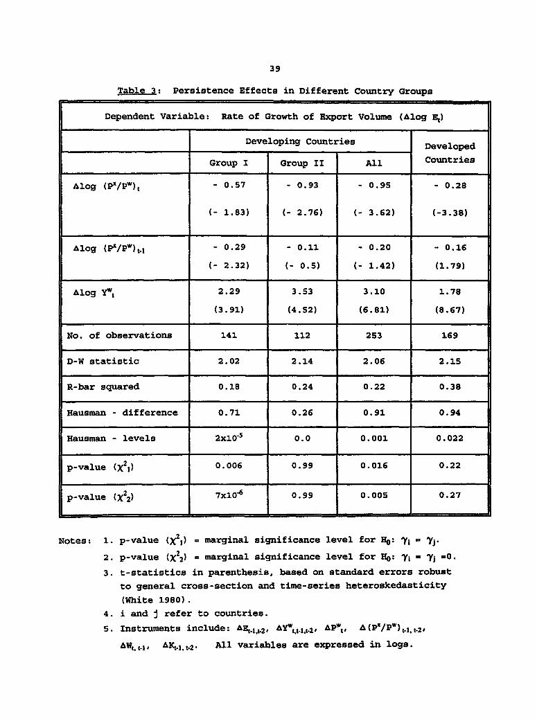
Table 3 shows that country-specific fixed effects are significantly

different from each other in Group I, the p-value of the X2-statistic is 0.006.

As can be expected, the fixed effects terms obtained for individual countries are

now different from the ones obtained from pooling all developing countries.

However, the orders of magnitude and relative rankings are verv similar (compare

the first and the last columns in table 2). The persistent growth rates of

Indonesia and Turkey are 19 and 17 percent, respectively, whereas Korea's is 12

percent. When equation 1 is estimated for Group I countries, Portugal's fixed

effects term becomes positive (in contrast to the result when it is estimated for

all developing countries, see Table 2).

Group II countries have negligible country-specific fixed effects

when considered as a group, though some have individually negative residual

growth rates. India, for example, records -3 percent. Venezuela has a

relatively high 3.3 percent; however, the time pattern of the growth rate is

erratic, in part because its exports tend to be dominated by petroleum-related

products. Accordingly we keep it in Group II.

13

Note also from table 3 that the income elasticity of demand is lower

for the products from developed countries than the ones from developing countries

-- this is commonly observed and attributed to the inclusion of high-growth

countries in the developing country sample. However, Table 3 shows that the

difference between developed and developing countries' income elasticities

originates in part from the high elasticity for the Group II countries (3.53),

which have low export growth rates and, typically, negative fixed effects. The

paradox of high income elasticities in Group II countries is discussed in Section

III, leading to a new interpretation of conventionally estimated income

elasticities.

C. Persistence

To study changes in the country-specific fixed effects over time, we

create seven-year overlapping "windows" in our sample period. The first window

covers 1972-1978, the second: 1973-1979, the third: 1974-1980, and so on. We

thus have eight windows. For each window we estimate the export demand equation.

For each country, therefore, we obtain eight yis. (See Figure 1, where it should

be noted that year refers to the final year of the window.)

Despite fluctuations, most countries in Group II (Argentina,

Colombia, Chile, India, Pakistan, Yugoslavia, and Israel) had low fixed effects

throughout the period (Figure la) ; in contrast, most countries in Group I

(South Korea, Singapore, Brazil, Malaysia, Thailand, Philippines, Spain, and

Greece) had relatively high fixed effects (Figure lb).

14

However, both increasing and decreasing trends are also discernible,

indicating that the groups are not closed. Indonesia, Turkey, Portugal,

Venezuela, and Mexico have steadily increased the size of their fixed effects

(Figure ic). Significant realignments occurred from 1981 to 1983, during a

severe downturn in global economic activity. In these years, some of the East

Asian newly industrializing economies (such as Korea, Singapore, and Taiwan)

experienced rapid wage growth. Countries that increased their fixed effects

coefficients during those years have continued to increase them. A number of

countries suffered a sharp decline in fixed effects coefficients during that

period and have not recovered: most of these were countries that already had low

fixed effects -- India, Israel, Argentina, Chile, Colombia, and Yugoslavia;

however, Greece and Philippines also suffered.

Further, in the early 1980s, estimated fixed effects coefficients of

countries that performed very well in the 1970s, including South Korea,

Singapore, Brazil, Malaysia and Thailand began to decline (Figure lb). If the

high fixed effects term represents the transition from outsider status to the

ranks of the insiders, a decline in the fixed effect toward zero represents their

maturity as insiders.

We draw three inferences from these observations. First, the growth

of exports due to unobserved factors tends to persist over time within a country.

Second, when underlying cost conditions change, and for instance, Group I

countries become expensive producers, new entrants are likely to gain. Third,

these shifts take place over time but can be accentuated by downturns in the

15

world economy. During such periods international buyers seek new suppliers.

Firms and countries that are well-positioned in such years stand to make large

gains.

D. Mismeasurement and Incorrect Instruments

Since the country-specific persistent influences could be merely a

reflection of errors in measuring the relevant price and income variables, it is

necessary to take into account the proposition that if all variables were

correctly measured, the observed persistence would disappear. The implication

would be that price and/or income elasticities are much higher than typically

estimated. A similar argument would hold if the simultaneous determination of

export prices and volumes was not fAlly accounted for. The use of incorrect

instruments for relative price in the export demand function would lower the

(absolute) value of the price elasticity of demand.

A common problem in estimating export demand functions is that the

price variable is not measured correctly. The unit values typically used, as is

the case here, do not account adequately for changes in the composition of

exports. Thus, for countries that shift toward products with higher prices per

unit of product sold (from t-shirts to televisions), the unit value index

understates the price increase (See Alterman 1991, who finds that this has been

the case for U.S. imports from some developing countries).

Other factors will lead to an overstatement of the price change by

the unit value index. If new products include an increasing fraction of a

16

country's exports, the true price index for the enlarged bundle of goods will be

lower than the conventionally measured index (see Feenstra 1992). The effect

of the increased bundle of goods is identical to unmeasured quality improvements

or greater "taste" for that country's goods in world markets. Feenstra (1992)

has attempted to construct price indices that reflect the introduction of new

products and the exit of old products in the goods supplied by developing

countries. As noted, Helkie and Hooper (1988) use a more direct (though more

approximate) approach by including in their demand function the capital stock of

the supplying country as a proxy for the ability to supply new products.

In our estimates, the measurement problem is alleviated by the use

of instrumental variables and by data transformation. In correcting for

simultaneity, we use wage rates and other proxies for production conditions as

instruments. In general, the solution for simultaneity is the same as that for

measurement error, and we have, in principle, corrected for simultaneity. The

question is whether our correction is adequate. Specifically, have we adequately

accounted for influences on the supply of exports? If not, the persistence being

picked up in the demand function could well be the result of ignoring supply

factors rather than a feature of the demand function.

We do not believe that it will be possible to fully resolve the

question of whether the observed persistence derives from supply or demand

factors. However, additional results suggest that while we have not fully

accounted for all supply influences, efforts at refining the export supply

17

equation are not likely to have much power in eliminating the persistence effects

observed.

To test the sensitivity of our results to the choice of instruments,

we experimented with dropping instruments individually or in groups. The overall

conclusion is that neither the elasticities nor the fixed effects coefficients

change significantly. Only when the world price was dropped from the list of

instruments, the estimated price elasticity of the Group I countries increased,

with no significant effect on the country-specific constant terms.

These results are similar to those obtained by Feenstra (1992). In

a more sophisticated correction of price changes, he finds that the quality-

adjusted price for many developing countries rose more slowly than conventional

estimates suggest. The correction leads, in his case, to a higher price

elasticity of demand and a lower income elasticity, although the changes are

limited in magnitude.

A second approach to dealing with measurement errors is through the

transformation of data. At least since Griliches and Hausman (1986), it has been

known that specific transformations of panel data can be used to minimize the

influence of measurement errors; it is also the case, however, that certain

transformations of the data can exacerbate measurement errors. We measure the

variables as rates of change (first differences of log values), a procedure that

is generally considered to increase the "noise-to-signal" ratio, if the variable

under consideration is serially correlated. However, Griliches and Hausman (p.

100) note that if the measurement error, rather than the variable itself, is

18

serially correlated, then first-differencing helps to reduce the noise and to

increase the signal. In our situation, we can expect the measurement errors to

be highly positively correlated, since quality and compositional changes in

exports are not random effects that vary from year to year, but represent changes

over time. This is at least partially borne out by the figures in Alterman

(1991), in which unit value indices are compared with "true" price indices: the

errors show significant positive serial correlation. Thus first-differencing is

likely to be an effective method of reducing measurement errors.

Griliches and Hausman (1986) propose a test to determine whether the

presence of measurement errors is a source of bias in parameter estimates. The

test involves a statistical comparison of the GLS (random effects) and the fixed

effects (within) estimators.

Adapting their framework and allowing for the possibility that the

unit values reflect export prices only partially, we write the percentage change

in the export unit value (AIh) as the sum of the percentage change in the

unobserved export price (,Pit) and the measurement error (v1t): AIt = AP,t+vk. When

the export demand equation (equation 1) is estimated with AI;, and AI; t-. rather

than the true price variables, the residual term will incorporate a vt + a1vi.,

which will be correlated with AIft and AIj,t-l. If the measurement errors are

negligible and there are no other sources of correlation between the residuals

and the unit values, both models (GLS and fixed effects) will be unbiased and

consistent; more importantly the parameter estimates from the two models (GLS

and fixed effects) will be asymptotically equal. However, when the correlation

19

between the composite residual term and the observed export unit value is

statistically significant, both models will produce biased parameter estimates

and these estimates will not be close to each other. As a result, it is possible

to test for the statistical significance of measurement errors indirectly via a

test for the equivalence of the GLS and the fixed effect estimates using the

Hausman specification test (Griliches and Hausman 1986).

P-values for the Hausman test (which has a x2 distribution under the

null hypothesis) are reported in Table 3 for both the first difference and the

levels estimation. The test results show that the first-differences model is not

plagued by the use of unit'value indices. In contrast, however, we cannot reach

the same conclusion for the levels estimation. Hausman tests for all country

groups have very small p-values, which implies that the levels estimation

produces biased estimates due to measurement errors; the highest p-value is

obtained for the developed countries. This result is consistent with the fact

that the composition of exports from developed countries is more stablP over time

compared to exports from developing countries, and that the quality of the data

from developed countries is higher.

III. Asvmmetries in Income Elasticity: Insiders and Outsiders

Traditionally, the effect of non-price factors is thought to be

captured by the response of exports to changes in world income (summarized in P,

the income elasticity of demand). A high income elasticity of demand is

20

considered a measure of superior quality, although as noted, the relationship

does not seem obvious from table 3. The income elasticity of demand for products

from developing countries is much higher than that from developed countries.

Should that be read to imply that developing countries export higher quality

products? Within developing countries, it is much higher for the lagging Group

II countries than for the dynamic Group I countries.

Krugman (1989) suggests that the observed high income elasticity of

demand for Japanese products reflects that country's ability to rapidly increase

the variety of products sold on world markets. Muscatelli, Srinivasan, and Vines

(1992) similarly suggest that Korea, Taiwan, and Hong Kong have benefitted

through expanding the range of products for sale. However, as noted, our

estimates show that the slow-growing (Group II) countries have a higher income

elasticity than the Group I countries, which is contrary to what would be

expected if income elasticity were a good measure either of product quality or

of expanding product variety.

The paradox is resolved when we consider the possibility that exports

respond asymmetrically to changes in world demand. We test the proposition that

income elasticity is different when world income rises than when it falls in the

following equationYV:

More refined non-linear responses could be tested but the results presentedare striking enough. The years in which world income fell were: 1974, 1975, and1982.

21

(2) AlogLie = yi £0 Aog(Pt/P¢) + a 1Alog(e ,w,/P'.)

+ V (AlogY7eV + + 1*- [AlogY7eV

where:

AlogY' if AlogY P0(AlogYl =

O otherwise.

AlogYr if AlogYl<O(AlogY'V ={(

O otherwise.

The effects of world income change are sharply asymmetric (table 4). In years

of rising income, the elasticities (P+) for the different groups of countries

are fairly close -- between 1.51 and 1.84.' The response to a decline in world

income, however, is much higher and more heterogenous.

The difference between income elasticities when incomes rise ana fall

is small and statistically insignificant. In the case of developed countries,

the p-value for the x2 test is 0.22, substantial for Group I countries but not

significant at the 5 percent significance level, and large and significant for

Group II countries with a p-value of 0.023. When world income rise by 1

7/ For Group II countries, P+ are barely statistically different from zero atthe 10 percent level of significance; however, it is not statistically different

from the corresponding elasticity for Group I and developed countries at the Spercent level of significance. The data continue to support the estimation of

demand equations separately for Group I and Group II countries, rather than forall developing countries. However, compared to the original demand equation theF-statistic is low at 2.41 with a p-value of 0.049, which implies that the modelwith pooled developing countries can be rejected only at the 5 percentsignificance level.

22

percent, exports of Group II countries increase by almost 2 percent (0+=1.84);

but when world income falls by 1 percent, exports from these countries decline

by 14 percent (P-=14.0). Thus, in times of rising incomes, all countries gain

equally in terms of export growth. When world income declines, however, the

Group II countries are hit the hardest; since they do not enjoy any special

advantage when the upturn occurs, they lose market share over time.

If product characteristics were the main factor in determining

elasticity, one would expect that when incomes fall, expenditure on luxury

products would register the sharpest decline. Thus we would conclude that 1-

should be the higheet for developed countries, instead of which, it is actually

the lowest. Similarly, if the Group II countries are supplying basic products

that account for a low share of the incomes of consumers, their exports would

hardly be affected by a decline in world income.

The ordering of a- can be better explained in terms of the demand for

adherence to delivery standards and long-term buyer-supplier relationships, as

discussed in Section V. when global demand declines, profit margins shrink and

buyers are more sensitive to product reliability and delivery schedules. Thus

they rely to a much greater extent on suppliers with a strong track record than

they would in periods of strong demand and higher profit margins.

Moreover, buyers invest in long-term relationships. The cost of

breaking a relationship is particularly high when ties are strong. Buyers in

industrial countries, who generate about two-thirds of the world demand for

manufactured exports, have strong relationships with other industrial countries

23

(Hakansson 1987); relationships are weakest in Group II countries, and are easily

broken. The marginal supplier is the first to lose an order. Such asymmetric

effects, which reflect the different costs of breaking relationships, have also

been noted in the context of the insider-outsider theory of labor markets

(Lindbeck and Snower 1988, Chapter 9).

For countries seeking to enhance their presence in international

markets, therefore, it is particularly critical to perform well during periods

of slowing or declining world demand. Growth in exports when world demand is

growing is relatively easy and does not contribute significantly to increased

market share. Maintaining market share when world income is growing slowly or

falling is of much greater value in terms of increasing long-term buyer interest.

These results also show that conventional measures of income

elasticity that do not disentangle the asymmetry discussed can lead to erroneous

interpretations. Landesmann and Snell (1989), for example, find that the income

elasticity of demand for manufactured exports from the United Kingdom has been

rising, which they assume implies greater non-price competitiveness. It is

curious, however, that during this period (late 1981 and 1982), the U.K. Is share

of exports in world trade fell quite precipitously and declined even further in

the next five years (Landesmann and Snell 1989, figure 3).

Our interpretation is that U.K. exports have performed poorly during

global downturns. The arithmetic average of a low elasticity when world income

expands and very high elasticity when income falls can be quite large. In this

case high income elasticity suggests that the U.K.'s non-price competitiveness

24

fell during the last decade. Our measure of non-price factors, y;, shows a clear

decline in the case of England.

In terms of method, therefore, this paper shows that commonly

estimated measures of income elasticity of demand can be very misleading. If the

asymmetric response of demand to rises and declines in income is not considered,

the high estimated income elasticity will be incorrectly interpreted as Implying

high product quality or an increasing variety of products.

IV. Telecommunications Penetration: A Proxy for Service Oualit ?

There are no simple physical correlates of a process by which new

buyers are drawn to a supplier. However, we attempt to demonstrate that

transactional quality (as proxied by the telecommunications infrastructure) is

important. We find that discontinuous shifts in transactional quality are needed

to make the jump from outsider to insider.

The number of telephone lines per capita is used, as a proxy for the

ability to communicate easily with buyers and to respond rapidly to their

requests. Note that this measure is mainly an indicator of the quality of the

transactions environment and not necessarily of the quality of the goods being

sold. To the extent that these are different, the measure is only a partial one.

Table 5 reports the regressions when the telecommunications variable

is added to the demand equation. To examine the possibility of endogeneity, both

the contemporaneous growth of telecommunications and growth in the previous year

are considered.

25

For Group I countries, we find the contemporaneous growth rate of

telecommunications penetration had no effect on export growth but growth in the

previous year had a positive effect on the growth of manufactured exports. The

elasticity of export growth with respect to growth in telecommunications is 0.54,

which is significantly different from zero at the 5 percent significance level.

More importantly, when telecommunications availability is introduced

as an independent explanatory variable, the fixed effects become much weaker.

As before, we use the X2-statistic to test the significance of the persistence.

Recall that when the telecommunications variable is not included as a right-hand

side variable, the X2-test strongly suggests the significance of the constant

term (or the average persistent growth rate) as well as the significance of the

individual fixed effects coefficients. When the telecommunications variable is

introduced directly into the demand equation, however, the p-values for both of

the X2-tests rise to 0.08. The significance levels, however, are sensitive to

the specification of the demand function. Thus when we allow for asymmetric

income elasticities, the p-value of the X2-test for the significance of country-

specific fixed effects is 0.02. Thus, while telecommunications growth is

strongly related to export growth in Group I countries, it does not conclusively

account for the country-specific effects.

The result is useful, however, because it points us in a direction

that provides an intuitively acceptable explanation of persistence. Two

observations are relevant in this regard. First, regardless of the exact

specification, with the inclusion of telecommunications as an explanatory

26

variable, the magnitude of the fixed effects coefficients falls for all countries

and in some--notably Korea--the fixed effects term almost disappears. In

Indonesia and Turkey, the two most dynamic countries in the sample, the fixed

effects decline but remain large. Second, table 6 shows that countries with high

export persistence have high average growth rates of telecommunications networks.

For Group II countries (with low and negative) fixed effects, table

5 shows that the contemporary telecommunications penetration has a positive

effect on export growth and the coefficient is significant at the 10 percent

level. A contemporaneous link could well be the result of more rapid exports

resulting in greater telecommunications investment. If that is the case, the

contemporaneous coefficient will be biased upward. To test for that possibility,

we also examine the relationship between the lagged value of telecommunications

penetration and export growth. Lagged telecommunications growth appears to have

no effect on export growth in this set of countries; the coefficient is negative

and insignificant with a t-statistic of -0.35. The evidence is, therefore, very

suggestive of the possibility that indeed the causality runs from export growth

to telecommunications investment.

To summarize, while the direction of causality in either case remains

uncertain, Group I countries have had high export and telecommunications growth

rates, whereas Group II countries have experienced low growth in both respects.

It is tempting to infer that a certain acceleration in growth, or a "push," in

either of the two variables is required to move from the low-growth to the high-

growth cycle. Although such a push could be successful in situations where the

27

capability of exporters to respond consistently with internationally marketable

goods is high, it could also lead to waste.

Note that the approach adopted in this section is similar to that of

Helkie and Hooper (1988) who take the stock of capital in the economy as a proxy

for the supply of a larger variety of goods. We focus on just telecommunications

because it is likely to be more germane to export activity. Moreover, for the

same reason, we prefer to think of telecommunications variable in the demand

equation as a measure of transactional quality rather than as a measure of

ability to supply an increased variety of goods.

V. A Descrintive Model of Diffusion and Lona-Term Contracts

If persistent growth rates are not artifacts, what omitted export-

inducing explanatory variables do they reflect? Why are the influences of the

omitted variables not captured in high (or low) income elasticities of demand?

And why do they instead appear as unidentified country-specific residuals?

The country fixed effects term reflects the influence of non-price

factors that are not captured by world income. As distinct from short-term

changes in demand because of world income changes, the fixed effects term is a

measure of the secular increase in a country's market share. Thus, the existence

of a positive country-specific fixed effect represents a diffusion of demand for

t.e country's products, that occurs when new buyers are attracted or when

existing buyers shift demand from other suppliers.

Product-cycle theories (Vernon 1966 and Krugman 1979) would predict

28

that the demand for specific croods shifts from developed country suppliers to

developing country suppliers who operate with lower wage costs; in our estimates,

however, a shift in the market share of all manufactured exports is implicit.

The shift, therefore, represents more than a simple product-cycle effect;

countries that benefit from this shift in demand are being transformed from

"outsiders" to "insiders" in the world trading system: thus, they sell to a

greater number of buyers and they sell a larger variety of goods.

Buyers "sample" products from different firms in different countries

and make inferences about quality and delivery standards. In purchasing

manufactured goods (especially time- and fashion-sensitive items, such as

clothes, shoes, bicycles, televisions) the dimensions of quality sought by a

buyer are: adherence to specifications, rimely delivery, and ease of

communications; good communications are essential for quick changes in production

and delivery (see Boatman 1991 and Pashigian 1988).

A few samples of poor quality can break the links between buyer and

supplier (even a single bad sample will do this, if the prior reputation is very

unfavorable). Good samples increase confidence in the supplier. The buyer, of

course, is anxious to choose a source as costs are incurred during the sampling

process. At some point, the buyer will select from those he perceives to be good

suppliers. Mistakes are possible, however, because sampling is not a perfect

predictor.

Once the decision is made, buying offices will be established, local

agents will be recruited, and relationships with suppliers will be formed. At

29

this stage, the buyer has an incentive to improve the performance of his supplier

and is likely to provide information and support to reinforce the suppliers,

strong points. Not only is there a significant cost to making these commitments,

but it is also costly to abandon them. If the long-term relationships are not

used, their value depreciates rapidly and must be rebuilt. This process creates

the persistence in relationships that we have observed in our field work (Egan

and Mody 1992), and is consistent with the relative stability of the country-

specific fixed effects.F

This line of reasoning is closely related to the Roberts and Tybout

(1992) analysis of sunk costs in exporting. Those firms that have exported are

treated as having incurred the sunk costs, raising the probability of exporting

in the current period and in the future. Our findings suggest that in addition

to exporters incurring sunk costs, buyers (conditional on transactional quality)

also make sunk investments in the establishment of long-term relationships with

their suppliers. Both buyers and sellers, therefore, have an incentive to

maintain their relationship, contributing to persistence in export growth.

Persistence in trade flows has also been examined in the context of

Y In the statistical literature, the process of sampling described isreferred to as the two- (or multi-) armed bandit problem. The analogyrefers to slot machines which have more than one arm, each with adifferent pay off. It is optimal in this situation to sample from botharms for a limited period and then invest all resources on the one thatseems to have a better performance (see Degroot 1970). Cowan (1988) hasextended the multi-arm bandit problem to the situation we consider here:once a choice is made, further investment in the relationship reinforcesthe decision to stick to one's choice.

30

U.S. trade by Krugman and Baldwin (1987), and their interpretation is similar to

ours. They argue that export prices react only with long lags to changes in

exchange rates and that trade volumes react only with long lags to export prices.

They use the "Book of the Month Club" analogy to explain these lags: once buyers

subscribe to a particular club, relative price changes do not cause them to

abandon the club unless these price changes persist.

A similar pattern of persistence is found in labor markets.

"Insiders" in the labor market are experienced workers who are hard to fire

because they are more productive, have legal contracts that are expensive to buy,

and work as a team. "Outsiders" are costly to identify and train. A consequence

of insider power is that wage and employment levels tend to persist. The degree

of persistence is not unlimited and if wage differentials between insiders and

outsiders become too large, a reshuffling can occur (see Lindbeck and Snower

1988).

VI. Conclusions

Growth rates of manufactured exports from developing countries tend

to be persistent,.although not immutable. In addition to the price and income

elasticities, a country's exports are partially influenced by the quality of its

transactional infrastructure (proxied by telecommunications penetration). More

importantly, we find indirecr evidence of "insiders" and "outsiders" in the world

market for manufactured goods, a condition that tends to perpetuate itself.

An asymmetry in the income elasticity of demand is related to the

31

persistence of export growth. The magnitude of the decline in exports following

a fall in world income is greater than the rise following an increase in world

income. The degree of asymmetry is greatest for marginal exporters (outsiders),

who are hardest hit from a drop in world income; these are also the countries

that face persistently low or negative growth rates. In contrast, developing

countries with persistently high underlying growth rates suffer a milder setback

when world income drops. Thus, countries with high persistent growth rates are

beneficiaries of a secular shift in demand, which reflects their changing status

from marginal to long-term suppliers.

This descriptive account is consistent with the hypothesis that

international buyers invest in long-term relationships to ensure product quality

and reliable delivery, and use these relationships to transfer production and

marketing knowledge to their suppliers. The resulting network of relationships

creates social capital that makes it costly to change buying patterns. Hence the

stability in buying relationships is broken mainly when production conditions

change significantly. The limited number of countries that are able to change

their status from outsiders to insiders experience explosive growth. Once their

insider status is established growth tends to level off. The evidence also shows

that countries that appear to have acquired such social capital have further

benefitted from physical investment in their transactional infrastructure.

Many theoretical models and export development strategies assume that

developing and newly industrializing economies, which are small in relation to

the world economy, can rapidly expand exports if domestic supply constraints are

32

removed. The results here do not support the notion that demand for developing

country exports is infinitely price elastic; neither do they imply elasticity

"pessimism." A price elasticity of about 1 is observed, large enough that policy

efforts to change relative prices should have a significant effect on export

growth. From a methodological point of view, the paper supports Feenstra's

conclusion that efforts at refining measures of relative price lead to only small

changes in the elasticities.

The paper's main point is that price-related measures, such as

devaluation or export subsidies, will have limited effects unless backed up by

infrastructure that makes the country an efficient and reliable supplier. These

attributes are of great importance for international buyers. The argument for

the overwhelming role of price as a determinant of export competitiveness is

certainly open to question. Riedel (1988b) points to Turkey as an example of the

benefits of trade liberalization and export subsidies, but it is worth noting

that Turkey's exports have also been supported by a massive effort to improve the

predictability of suppliers and expand the country's telecommunications network.

This is not to infer that a sophisticated telecommunications network

is the simple answer to export development. Telecommunications penetration is

not a fully satisfactory proxy for service quality. Moreover, in the case of the

slower-growing, Group II countries, the evidence suggests that exports induce

telecommunications investment rather than the other way around. The implication

for these countries is that mere reliance on telecommunications expansion as an

instrument for expanding exports is likely to result in disappointment. Building

33

long-term export relationships with international buyers also require the

capacity to deliver reliable products on time.

The findings imply that effective microeconomic institutional reforms

that improve the ease with which transactions are accomplished, together with an

enhanced ability to meet the exacting demands of world markets are critical to

export success. Such reforms cannot be achieved at once, and self-correction may

be required to improve performance.

34

REFERENCES

Aw, Bee Yan. 1992. "An Empirical Model of Mark-ups in a Quality Differentiated

Export Market." Journal of International Economics 33: 327-344.

Alterman, William. 1991. "Price Trends in U.S. Trade: New Data, New Insights.",

In Peter Hooper and J. David Richardson. eds. International Economic

Transactions: Issues in Measurement and Empirical Research. Chicago: The

University of Chicago Press.

Benhabib, Jess, and Boyan Jovanovic. 1991. "Externalities and Growth Accounting."

American Economic Review 81: 82-113.

Bhalla, Surjit. 1989. "Indian exports, imports, and exchange rates: a comparative

quantitative analysis." mimeo. World Bank, Washington.

Boatman, Kara T. 1991. Telecommunications and Export Performance: An Empirical

Investigation of Develorincr Countries. Ph.D Dissertation: University of

Maryland, College Park, Maryland.

Cowan, Robin. 1988. "Backing the Wrong Horse: Sequential Choice Among

Technologies of Unknown Merit." mimeo. Stanford University.

DeGroot, Morris H. 1970. Optimal Statistical Decisions. McGraw Hill Book Company.

Egan, Mary Lou and Ashoka Mody. 1992. "Buyer-Seller Links in Export Development.

World Development 20 (3): 321-334.

Feenstra, Robert C. 1992. "New Product Varieties and the Measurement of

International Prices." University of California, Davis.

Griliches, Zvi and Jerry A. Hausman. 1986. "Errors in Variables in Panel Data."

Journal of Econometrics 31: 93-118.

Hakansson, Hakan. 1987. Industrial Technolocrv: A Network AoDroach. Croom Helm.

Helkie, William H. and Peter Hooper. 1988. "The U.S. External Deficit in the

1980s: An Empirical Analysis." In R.C. Bryant, G. Holtham, and P. Hooper. eds.

External Deficits and the Dollar: The Pit and the Pendulum. Washington D.C.: The

Brookings Institution.

Krugman, Paul. 1979. "A Model of Innovation, Technology Transfer and the World

Distribution of Income." Journal of Political Economy 87: 253-266.

35

Krugman, Paul. 1989. "Income Elasticities and Real Exchange Rates." European

Economic Review 33: 1031-54.

Krugman, Paul and Richard Baldwin. 1987. "The persistence of the U.S. trade

deficit." Brookings Paners on Economic Activity 1: 1-55.

Landesmann, Michael and Andrew Snell. 1989. "The consequer.ces of Mrs. Thatcher

for U.K. Manufacturing Exports." Economic Journal 99, 1-27.

Lindbeck, Assar and Dennis J. Snower. 1988. The Insider-Outsider Theory of

Emtlovment and UnemDlovment. Cambridge: MIT Press.

Marquez, J. and C. McNeilly. 1988. "Income and Price Elasticities for Exports of

Developing Countries." Review of Economics and Statistics 70: 306-314.

Muscatelli, V.A., T.G. Srinivasan, and D. Vines. 1992. "Demand and supply factors

in the determination of NIE exports: a simultaneous error-correction model for

Hong Kong." Economic Journal 102, 1467-1477.

Pashigian, B. Peter. 1988. "Demand Uncertainty and Sales: A Study of Fashion and

Markdown Pricing." American Ero Cmic Review. 78: 936-953.

Riedel, James. 1988a. "The Demand for LDC Exports of Manufactures: Estimates from

Hong Kong." Economic Journal 98: 138-148.

Riedel, James. 1988b. "Strategy Wars: The State of Debate on Trade and

Industrialization in Developing Countries." Presented at Symposium in Honor of

Jagdish Bhagwati, Erasmus University, Rotterdam.

Roberts, Mark and James Tybout. 1992. "Sunk Costs and the Decision to Export in

Colombia." mimeo. Pennsylvania State University and Georgetown University.

Vernon, Raymond. 1966. "International Investment and International Trade in the

Product Cycle." Ouarterly Journal of Economics 80: 190-207.

36

APP8NDIX: Definition of Variables and Data Sources

P' : Unit value index for manufactured exports,

World Tables (WT), 1980100, US dollar based.

pW: Unit value index for worldwide exports of manufactured goods,

GATT: International Trade, 1987-1988, 1980=100.

W : Nominal wage rate, ( - RW * GDP deflator ),

RW : real earnings per employee in manufacturing, WT, 1980=100;

GDP deflator : WT, 1980=100, local prices.

e : Nominal exchange rate, index, WT, conversion factor(annual average).

B : Exports of manufactured goods, WT, constant 1980 US dollars.

Yw : World GDP, defined as

94

r siyi

where YJ is the GDP of the ith partner of the country i, in constant

1980 US dollars, and sJi is the average share of partner j in the total

exports of i throughout the period:

and E'i : Manufactured goods exports from ith country to its jth

partner, constant 1980 US dollars. Manufacturing sector covers all

products from SITC 5 to SITC 8 minus SITC 68. Source: United Nations,

Comtrade Database.

K : Capital good imports, constant 1980 US dollars.

Data from Comtrade database ( = 71 + 72, SITC ) in current prices, US

dollars, are deflated by the price index for worldwide capital good imports

from UN Statistical Bulletin, 1970-87.

T Telephone stations (sets) of all kinds per 100 inhabitants.

Data series 9.1, from The Yearbook of Common Carrier Telecommunications

Statistics, various issues.

37

Table 1: Export Demand Fur.ctions for Developing Countries

Dependent Variable: Rate of Growth of Export Volume (&log E,)

Country-specific Yi = zj Fi - 0

7'Y

Alog (P/PW)t - 0.95 - 1.01 - 1.08

(- 3.62) (- 3.46) (- 3.66)

slog (px/pw) 1 1 - 0.20 - 0.21 - 0.12

(- 1.42) (- 1.58) (- 0.87)

Alog ywt 3.10 3.10 4.14

(6.81.) (6.38) (12.45)

Constant (7) 20.044 _

(2.67)

No. of observations 253 253 253

D-W statistic 2.06 1.85 1.79

R-bar squared 0.22 0.18 0.16

p-value (X21) 0.016 _

p-value (X 2) 0.005

Notes: 1. p-value (X2i) - marginal significance level for HO: 7y = yj.

2. p-value (X22) - marginal significance level for Hb: yi yj =0.

3. t-statistics in parenthesis, based on standard errors robustto general cross-section and time-series heteroskedasticity

(White 1980).

4. i and j refer to countries.

5. Instruments include: AE1.1 t.2, AYw,tl.2 APw A (pX/Pw)t - .2'

AW, t-.1, A*Ktl, t.2- All variables are expressed in logs.

38

Table 2: Quantitative Importance of Country Specific Fixed Effects

Country-specific Actual Growth rate Relative importance Country-specificgrowth rate growth rate without country- of country-specific growth rate

(pooled) specific effects effect (separate groups)(2) (4) = (1)/(2) (5)

(1) ~~~~~~~~(3) =(2) - (1)

Brazil 6.6 16.5 9.9 0.40 9.2

Greece 2.1 10.4 8.3 0.20 4.2

Indonesia 16.9 26.3 9.4 0.64 19.2

South Korea 8.9 17.0 8.1 0.52 10.9

Malaysia 10.4 15.4 5.0 0.68 11.8

PhDippines 14.3 18.7 4.4 0.76 16.1

Porugal -0.6 7.3 7.9 -0.08 1.5

Singapore 6.2 12.6 6.4 0.49 7.8

Spain 1.4 9.9 8.5 0.15 3.7

Thailand 6.7 13.7 7.0 0.49 8.5

Turkey 16.2 21.7 5.5 0.75 17.6

Argenine -0.5 2.8 3.3 -0.18 -1.7

Chile -0.1 7.5 7.6 -0.02 -1.1

Colombia -0.25 3.8 6.3 -0.67 -3.9

India -2.3 3.7 6.0 -0.61 -3.6

Israel 3.3 11.7 8.4 0.28 2.6

Mexico -3.2 3.1 6.3 -1.04 -4.5

Pakistan 1.3 8.7 7.4 0.15 0.2

Venmzuela 3.6 14.4 10.8 0.25 2.7

Yugoslavia 0.6 5.6 5.0 0.11 -0.7

Note: Country-specific growth rates (column 1) are the corresponding fixed-

effect terms from the pooled estimation of equation 1 for 20 developing

countries in our sample. Country-specific growth rates in Column 5 are the

fixed effects terms from separate estimations for Group I and II countries.

39

Table 3: Persistence Effects in Different Country Groups

Dependent Variable: Rate of Growth of Export Volume (Alog Et)

Developing Countries Developed

Group I Group II All Countries

Alog (px/pw) - 0.57 - 0.93 _ 0.95 - 0.28

(- 1.83) (- 2.76) (- 3.62) (-3.38)

Alog (PK/PW)1 1 - 0.29 - 0.11 - 0.20 - 0.16

( 2.32) (- 0.5) (- 1.42) (1.79)

Alog Ywt 2.29 3.53 3.10 1.78

(3.91) (4.52) (6.81) (8.67)

No. of observations 141 112 253 169

D-W statistic 2.02 2.14 2.06 2.15

R-bar squared 0.18 0.24 0.22 0.38

Hausman - difference 0.71 0.26 0.91 0.94

Hausman - levels 2x10-5 0.0 0.001 0.022

p-value (X21) 0.006 0.99 0.016 0.22

p-value (X22) 7x104 0.99 0.005 0.27

Notes: 1. p-value (x 21) * marginal significance level for Hi: y = j

2. p-value (X22) = marginal significance level for HO: yl - Tj =0.

3. t-statistics in parenthesis, based on standard errors robust

to general cross-section and time-series heteroskedasticity

(White 1980).


5. Instruments include: AE_t.2, AYWt.ttlt2, APwt, A (P[/PW) t-1. t-2'

AWtt1, AKt1. t-2* All variables are expressed in logs.

40

Table 4: Asymmetries in Income Elasticity

Dependent Variable: Rate of Growth of Export Volume (&log Et)

Developing Countries Developed

Group I Group II All Countries

Alog (px/pw) t 0.71 - 0.88 - 1.02 - 0.28

(- 2.23) (- 2.69) (- 3.93) (- 3.31)

Alog (p/pw) t- - 0.29 - 0.10 - 0.20 - 0.14

(- 2.36) (- 0.48) (- 1.52) (1.55)

[Alog yw 1]+ l.Sl 1.84 1.64 1.55

(2.05) (1.78) (2.65) (5.14)

[Alog Ywtl- 8.69 14.00 3.2.68 3.65

(2.43) (2.97) (_.97) (2.45)


D-W statistic 2.06 2.18 2.12 i.lO

R-bar squared 0.18 0.27 0.24 0.38

p-value (X 2 ;) 0.004 0.96 0.007 0.17

p-value (X22) 0.0001 0.90 0.0001 0.19

p-value (X 3) 0.069 0.023 0.002 0.22

Notes: 1. p-value (X21) = marginal significance level for HO: 'yi = yj.

2. p-value (X22) = marginal significance level for HO: yi = =0°

3. p-value (X23) = marginal significance level for go : B+ -.



(White 1980).


6. Instruments include: AEt_.t2, t AYwtt tA ( 1 / PW)t_. t.2,

AWt. t-l AKt-1. t-2 -All variables are expressed in logs.

41

Table 5: Telecommunications as a Proxy for Service Quality

Dependent Variable: Rate of Growth of Export Volume (Alog Et)

Group I Group II

Alog (PX/pw)1t 0.67 - 0.70 0 0.90 - 0.87

(- 2.09) (- 2.16) (- 2.52) (- 2.27)

Alog (PVP/w)tI - 0.30 - 0.35 - 0.15 - 0.10

(- 2.37) (- 2.97) (- 0.57) C- 0.4)

Alog YWt 2.32 2.43 3.51 3.27

(3.93) (4.14) (4.15) (3.85)

Alog Tt 0.13 - 0.85 _

(0.52) (1.63)

Alog Tt.i - 0.54 - 0.19

(2.13) (- 0.35)


D-W statistic 2.05 2.00 1.97 2.07

R-bar squared 0.17 0.21 0.28 0.23

p-value (%21) 0.062 0.077 .99 .99

p-value (X27) 0.035 0.083 .86 .99

Notes: 1. p-value (X'I) - marginal significance level for HO: y yj.

2. p-value (X22) - marginal significance level for HO: '=j yj =0.



(White 1980).


5. Instruments include: AEt,.It2 AYw t-t.,t2 APwt, A(PX/PW)t-l.t-2

AWt, t- AI S4, t-2; and ATt-I or ATt, depending on the equation

estimated. All variables are expressed in logs.

42

Table 6: Telecommunications Penetration Rates

Average 1971 1985 Average Group

1971-85 growth rate

Korea 9.67 2.10 25.50 0.15 I

Singapore 24.65 6.80 44.24 0.11 I

Turkey 4.21 1.62 9.07 0.10 I

Malaysia 4.66 1.61 9.08 0.09

Yugoslavia 8.10 3.59 NA 0.07 n

Thalnd 0.96 0.43 NA 0.09 I

Brazil 5.28 2.09 9.30 0.09 1

Mexico 6.20 3.12 NA 0.08 U

Greece 26.96 11.97 41.34 0.07 1

Indonesia 0.33 0.17 0.52 0.07 I

Spain 27.52 13.46 39.59 0.06 I

Israel 30.02 17.40 46.89 0.06 n

India 0.37 0.22 0.57 0.06 U

Philippines 1.20 0.65 NA 0.06

Pakistan 0.42 0.79 0.68 0.05 U

Portugal 13.65 8.50 20.48 0.05 I

Colombia 5.85 3.77 8.04 0.04 n

Argentina 9.10 6.81 11.60 0.03 n

Chile 5.03 4.01 6.51 0.03 n

Venezuela 6.13 3.70 8.19 0.02 n

All 9.51 4.64 17.6 0.159

Note: Number of telephone sets of all kinds per 100 inhabitants.

Figure 1: Residual Rate of Export Growth (1973-1985)

(a) Low0.35

0.3

0.25

0.2-

2 0.1s \ ~~~~ ~ ~ ~~~~~~~India tw

0.05

0

-0.05'

4.0.0 1970 1980 1981 1962 1983 184 1WS

(b) High0.35

0.3

0.25,

0.2

8 0.15

20.1 3 0.05-

O

.0.05

-0.11979 1980 1981 1982 1983 19t4 1985

(c) Increasing0.35

0.3_

0.05

0.2-

el80.1

-0.05.

1979 1980 1981 1982 1983 1984 1988

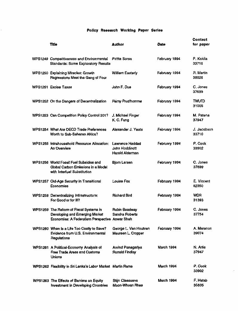
Policy Research Working Paper Serles

ContactTitle Author Date for paper

WPS1249 Competitiveness and Environmental Piritta Sorsa February 1994 P. KokilaStandards: Some Exploratory Results 33716

WPS1250 Explaining Miracles: Growth William Easterly February 1994 R. MartinRegressions Meet the Gang of Four 39026

WPS1251 Excise Taxes John F. Due February 1994 C. Jones37699

WPS1252 On the Dangers of Decentralization Remy Prud'homme February 1994 TWUTD31005

WPS1253 Can Competition Policy Control 301? J. Michael Finger February 1994 M. PatenaK. C. Fung 37947

WPS1254 What Are OECD Trade Preferences Alexander J. Yeats February 1994 J. JacobsonWorth to Sub-Saharan Africa? 33710

WPS1255 Intrahousehold Resource Allocation: Lawrence Haddad February 1994 P.CookAn Overview John Hoddinott 33902

Harold Alderman

WPS1256 World Fossil Fuel Subsidies and Bjom Larsen February 1994 C. JonesGlobal Caibon Emissions in a Model 37699with Interfuel Substitution

WPS1257 Old-Age Security in Transitional Louise Fox February 1994 E. VincentEconomies 82350

WPS1258 Decentralizing Infrastructure: Richard Bird February 1994 WDRFor Good or for III? 31393

WPS1259 The Reform of Fscal Systems in Robin Boadway February 1994 C. JonesDeveloping and Emerging Market Sandra Roberts 37754Economies: A Federalism Perspective Anwar Shah

WPS1260 When Is a Life Too Costly to Save? George L. Van Houtven February 1994 A. MaranonEvidence from U.S. Environmental Maureen L Cropper 39074Regulations

WPS1261 A Political-Economy Analysis ot Arvind Panagariya March 1994 N. ArtisFree Trade Areas and Customs Ronald Findlay 37947Unions

WPS1262 Flexibility in Sri Lanka!s Labor Market Martin Rama March 1994 P. Cook33902

WPS1263 The Effects of Barriers on Equity Stijn Claessens March 1994 F. HatabInvestment in Developing Countries Moon-Whoan Rhee 35835

Policy Research Working Paper Series

ContactTitle Author Date for paper

WPS1264 A Rock and a Hard Place: The Two J. Michael Finger March 1994 M. PateniaFaces of U.S. Trade Policy Toward 37947Korea

WPS1265 Parallel Exchange Rates in Miguel A. Kiguel March 1994 R. LuzDeveloping Countries: Lessons from Stephen A. O'Connell 34303Eight Case Studies

WPS1266 An Efficient Frontier for International Sudhakar Satyanarayan March 1994 D. GustafsonPortfolios with Commodity Assets Panos Varangis 33732

WPS1267 The Tax Base in Transition: The Case Zeljko Bogetic March 1994 F. Smithof Bulgaria Arye L. Hillman 36072

WPS1268 The Reform of Mechanisms for Eliana La Ferrara March 1994 N. ArtisForeign Exchange Allocation: Theory Gabriel Castillo 38010and Lessons from Sub-Saharan John NashAfrica

WPS1269 Union-Nonunion Wage Differentials Alexis Panagides March 1994 I. Conachyin the Developing World: A Case Harry Anthony Patrinos 33669Study of Mexico

WPS1270 How Land-Based Targeting Affects Martin Ravallion March 1994 P. CookRural Poverty Binayak Sen 33902

WPS1271 Measuring the Effect of External F. Desmond McCarthy March 1994 M. DivinoShocks and the Policy Response to J. Peter Neary 33739Them: Empirical Methodology Applied Giovanni Zanaldato the Philippines

WPS1272 The Value of Superfund Cleanups: Shreekant Gupta March 1994 A. MaranonEvidence from U.S. Environmental George Van Houtven 39074Protection Agency Decisions Maureen L Cropper

WPS1273 Desired Fertility and the Impact of Lant H. Pritchett March 1994 P. CookPopulation Policies Lawrence H. Summers 33902

WPS1274 The New Trade Theory and Its Asad Alam March 1994 A. AlamRelevance for Developing Countries 87380

WPS1275 Female-Headed Households, Ricardo Barros March 1994 K. BinkleyPoverty, and the Welfare of Children Louise Fox 81143in Urban Brazil

WPS1276 Is There Persistence in the Growth Ashoka Mody March 1994 M. Pateffaof Manufactured Exports? Evidence Kamil Yilmaz 37947from Newly Industrializing Countries

Asymmetry in the income elasticity, of demand, and t-- in ... · elasticity of demand, and from the...

Documents

Transcript of Asymmetry in the income elasticity, of demand, and t-- in ... · elasticity of demand, and from the...